For the second presidential election in a row the prediction of the “Klarner Model” was within half a percent of the actual result. This model forecast that Obama would receive 51.3% of the two-party vote, while he actually received 51.8%.Footnote ¹ The model also called all states correctly, with the exception of Florida, which was predicted to be narrowly lost by Obama with 49.7% of the vote. These forecasts were made on July 15, 2012. This success does not indicate the model is better than the other models in the symposium as luck is a major determinant of which model gets closest to the mark. Although the Klarner Model correctly called 49 out of 50 states, that means little in an election where merely calling states on the basis of 2008 results would have called all but two correctly.

Two other state-level presidential forecasting models were presented in the October PS election forecast symposium: that of Jerome and Jerome-Speziari (J&J), which called two states incorrectly, and that of Berry and Bickers (B&B), which called nine incorrectly. The accuracy of the J&J Model for the national popular vote was essentially tied with the Klarner Model, while B&B were 4.3% off. If we stopped here, we could conclude that the J&J Model did as well as the Klarner Model whereas the B&B Model did worse. However, all three models were equally unimpressive in one way, and the B&B Model brought information to the table that was not in a variety of other sources, as explained next.

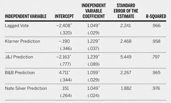
Making accurate forecasts at the state level is a function of two things: correctly calling the national tide and correctly ordering Democratic success across states. One standard of how good a model is at ordering the states is determined by its ability to add prediction success to a variable measuring the percent of the vote obtained by the Democrat in the last election. Table 1 reports the results of five regressions, with the dependent variable in all being the 2012 Democratic percent of the two-party vote. All variables are centered around 50% to facilitate assessment of bias.

Table 1

Five Regressions Assessing the Relationship between 2012 State Democratic Vote, Forecasts, and Lagged Vote

Note: standard error in parentheses.

^* = p < .05.

N = 51

The first regression reported in table 1, in row two, indicates that the 2008 vote accurately ordered the states from most to least Democratic. When using the predictions from the three state-level forecasts as independent variables (rows three, four, and five), none perform better than lagged vote. The fifth regression in the table uses Nate Silver's November 5, 2012, state predictions as an independent variable as a useful summary of forecasts from polls immediately before Election Day: it only marginally improves on 2008 vote share in its ability to order states, but this indicates that it is possible to improve over prior vote share. When the four forecasting variables are added to a model with lagged vote share in turn, only those of B&B and Silver attain statistical significance (analyses not shown). Perhaps the care that B&B took in modeling state economic conditions yielded predictive capacity not found in other sources. When pitted against Silver's Election Eve forecasts, their forecasts still attained statistical significance (p < .05, analyses not shown).

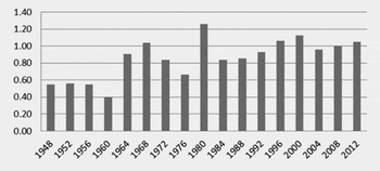
Figure 1 reports the unstandardized regression coefficient from bivariate regressions of the state Democratic two-party vote on lagged vote share for each of the 17 elections from 1948 to 2012, but excluding the “one party” states not used in the prediction model (Klarner Reference Klarner2012, 655). The figure indicates that the impact has gone up over time, while prediction error (measured by the standard error of the estimate from those 17 regressions, not shown) has gone down, with lagged vote doing better at predicting current vote in 2012 than any other postwar election. This trend is what one would expect with the increased polarization of the electorate over time. These findings suggest that the longer time period used in the Klarner Model may have decreased its ability to order states correctly from least to most Democratic, as it “overaggregates.” In contrast, the longer time period of the Klarner Model in comparison to the other two state-level models may have helped it call the national tide more accurately. Combining the advantages of both will be a goal for 2016.

Figure 1

Impact of Lagged Presidential Vote

The Klarner state-level US House Model predicted that the Republicans would pick up two seats and leave the Democrats with 191. In actuality, the Democrats won 200 seats, the Republicans 234, with the outcome of one race still undecided, making the model nine or ten seats off. Therefore, the US House Model performed reasonably well, as it did in 2006 and 2008.

The Klarner state-level US Senate Model did much worse. It predicted that after the election Democrats would have 48 seats (including Bernie Sanders), and the Republicans would have 51 (a forecast was not made for Maine). Actually, the Democrats were left with 54 seats, and the Republicans with 45, making the forecast six seats off. The Klarner US Senate Model has never performed well, being off by three seats in 2006 and five seats in 2008. US Senate elections appear to be influenced by race-specific factors that are difficult to include in forecasting models.