1. Introduction
High-Reynolds-number jet exhausts, like those from full-scale jet engines, can have remarkably thin shear layers between the relatively uniform exhaust plume and the slower ambient flow. The thickness depends on the specific flow conditions, but typically we expect that the jet will have a nozzle-diameter Reynolds number of over
 $10^{6}$
at application scales (Janardan et al.
Reference Janardan, Hoff, Barter, Martens, Gliebe, Mengle and Dalton2000). For confidence in engineering design, it is undoubtedly preferable to analyse configurations that match those of the target engineering applications as closely as possible. However, this is expensive for full-scale jet engines, which makes small-scale experiments and simulations attractive. Even for scale models with nozzle diameter
 $D=90~\text{mm}$
, the momentum thickness can be as small as
 ${\it\theta}/D=0.0009$
and is observed to be even smaller at full scale (Viswanathan & Clark Reference Viswanathan and Clark2004). This presents a challenge for both numerical simulations and testing in a model-scale facility where nozzles typically have still thicker shear layers
 ${\it\delta}/D$
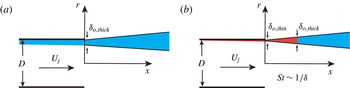
. As a result, there is a nominally missing region of noisy turbulence, such as visualised in figure 1. Superficially, this presumably results in missing sound sources, particularly some that might contribute to the high-Strouhal-number acoustic radiation. Furthermore, altering jet exit conditions is understood to affect flow development and noise (Maestrello & McDaid Reference Maestrello and McDaid1971; Hussain & Zedan Reference Hussain and Zedan1978; Zaman Reference Zaman1985a
,Reference Zaman
b
; Bridges & Hussain Reference Bridges and Hussain1987; Viswanathan & Clark Reference Viswanathan and Clark2004; Bogey & Bailly Reference Bogey and Bailly2010; Bogey, Marsden & Bailly Reference Bogey, Marsden and Bailly2011, Reference Bogey, Marsden and Bailly2012; Zaman Reference Zaman2012; Bogey & Marsden Reference Bogey and Marsden2013), which will in general also involve the dynamics in this thin region. These issues motivate this study. In addition, characterisation of thick nozzle boundary layer jets will enable accounting for this region when it cannot be explicitly represented in simulations or model-scale experiments. The near-nozzle flow is also particularly important because of its central role in noise suppression designs.
Schematic of mean boundary and shear layers for both (a) thick and (b) thin initial conditions.

1.1. Jet noise sources
Source localisation techniques have shown that the low-frequency components of the far-field sound spectrum appear to be generated primarily near the close of the potential core,
 $5\lesssim x/D\lesssim 10$
, whereas the corresponding high-frequency sound is primarily produced near the nozzle exit,
 $0\lesssim x/D\lesssim 3$
(Narayanan, Barber & Polak Reference Narayanan, Barber and Polak2002). This general behaviour reflects expectations based upon the largest turbulence scales, which will roughly match the jet diameter
 $D$
near the end of the potential core and the smaller shear-layer thickness
 ${\it\delta}$
near the nozzle. Given that these locally largest scales carry most of the turbulence energy, it can be anticipated that they will generate most of the acoustic energy from their respective regions of the flow. Statistical analysis of theoretical turbulence noise sources supports this (Lilley Reference Lilley, Hardin and Hussaini1993). The single length scale of self-similar mixing layers, which will be approximately realised near the nozzle exit, affords simplification of the statistical representation of the turbulence noise sources, and motivates in part the empirical similarity spectra of Tam, Golebiowski & Seiner (Reference Tam, Golebiowski and Seiner1996). In addition to setting the smallest shear length scale, the nozzle boundary layer thickness at its exit will also limit the onset of shear-layer self-similarity, the deviation from which should similarly disrupt self-similarity of sound spectra. We therefore also investigate the initial shear-layer development in our studies.
The convection velocity relation between
 ${\it\delta}$
and the largest turbulence scales also underlies models that attempt to represent sound-producing dynamics more explicitly. These have commonly involved a wavepacket representation of the largest turbulence structures, based upon linear stability models (Merkine & Liu Reference Merkine and Liu1975; Huerre & Crighton Reference Huerre and Crighton1983) or phenomenologically similar wave-like model sources (Ffowcs Williams & Kempton Reference Ffowcs Williams and Kempton1978; Crighton & Huerre Reference Crighton and Huerre1990). The instability mode character of these wavepacket structures implies an approximate relation between the local shear-layer thickness and their streamwise wavelength. Since the wavepackets will travel with a convection velocity
 $U_{c}$
that is approximately half the jet velocity
 $U_{j}$
, their Strouhal number will depend upon the local shear-layer thickness,
 $\mathit{St}\propto U_{c}/{\it\delta}$
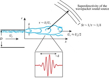
, which in turn links the the local thickness to the Strouhal number of the radiated sound (Jordan & Colonius Reference Jordan and Colonius2013) (see figure 2).
The near-nozzle exhaust region with some anticipated scalings (see text).

Of course, an actual turbulent jet shear-layer development is only approximately self-similar and its nonlinear turbulence will not just be made up of the relatively idealised wavepackets used to model its mechanisms. In general, anticipating the connection between turbulence and its radiated sound is even more challenging away from these quasi-equilibrium conditions. The nozzle will affect the turbulence for a distance downstream, delaying the onset of these better characterised regimes. For example, the transition region between a turbulent boundary layer of momentum thickness
 ${\it\theta}$
and self-similar shear layer, spans
 $150{\it\theta}$
downstream (Bradshaw Reference Bradshaw1966; Morris & Foss Reference Morris and Foss2003). For the thicker initial shear layers of model-scale experiments and some simulations, this
 $150{\it\theta}$
might extend far downstream, perhaps even the length of the potential core. Starting very close to the nozzle, we will quantify the developing shear layers of our high-speed jets. There is also an upstream effect of the nozzle exit (Sandberg, Sandham & Suponitsky Reference Sandberg, Sandham and Suponitsky2012), at least for a fully developed pipe flow upstream of the nozzle, though our diagnostics are restricted to quantify only its downstream consequences, which are the most important for noise generation.
1.2. Sensitivity to nozzle conditions
For simple round jets, the radiated noise is well-known to be sensitive to the laminar versus turbulent character of the nozzle boundary layers. Zaman (Reference Zaman1985a ) showed up to a 4 dB increase in radiated sound for a laminar versus a tripped and presumably turbulent initial shear layer. The mechanism responsible for this significant increase seems to be the pronounced amplification of linear instabilities supported by the small spreading angle of laminar flows and subsequent nonlinear saturation including possible vortex pairing dynamics. The resulting near-nozzle disturbances thus grow to be intense and relatively correlated, both of which will typically increase their acoustic radiation. Such significant differences have not been noted for turbulent shear layers, though it does not appear that a single-parameter family of initially turbulent jets has been studied and reported.
Viswanathan & Clark (Reference Viswanathan and Clark2004) report measurements for three nozzles: one with a cubic upstream contour, an ASME nozzle (ASME 1959) with the contraction forming a quarter of an ellipse followed by a straight section, and a conical nozzle with smooth transitions between sections. Their respective boundary layer thicknesses were estimated to vary by a factor of 3 as deduced from a Reynolds-averaged-Navier–Stokes solver with a
 ${\it\kappa}{-}{\it\epsilon}$
turbulence model. The sound pressure level (SPL) in the mid-frequency range, near Strouhal number
 $\mathit{St}_{D}=f\,D/U_{j}\approx 1$
, varied by about 3 dB, though it did not seem to have any direct relationship with these nozzle boundary layer thickness estimates, which were predicted to change as a consequence of the nozzle designs but were neither directly measured nor a specific point of investigation. One of our goals is to specifically quantify this aspect of the nozzle exit flow, with minimal other variation. Zaman (Reference Zaman2012) provides a pithy discussion of the complex interrelated issues of nozzle contour, turbulence condition, and related factors that might affect noise. We do not reproduce this discussion here, though we were mindful of these issues in crafting our designs. Indeed, a principal goal is to clarify these issues via our single-parameter family of nozzles and detailed measurement of the nearly identical turbulence statistics, when scaled by
 ${\it\delta}$
, in our initial shear layers despite their differing thicknesses.
1.3. Simulation-based prediction
The near-nozzle mechanics of jet noise presents a particular challenge in numerical simulations. The geometric flexibility afforded by such simulations is attractive but remains computationally expensive or even prohibitive for a number of reasons. The fundamental unsteadiness of noise sources and requisite fidelity are at the root of this expense. Lower cost statistical modelling of turbulence as a source of sound has been successful, but does not meet all current fidelity needs. A high-fidelity prediction seems to require that the turbulence be represented in some detail, presumably with large-eddy simulation techniques (Wang, Freund & Lele Reference Wang, Freund and Lele2006). We can anticipate, based on the observations reviewed above, that faithful representation of the near-nozzle turbulent shear layers is required, which will remain a challenge in such simulations. Early jet noise simulations coped with resolution challenges by having either an unrealistically thick turbulent inflow shear layer (Freund, Lele & Moin Reference Freund, Lele and Moin2000) or a thin but laminar inflow shear layer (Freund Reference Freund2001). Both approaches significantly reduce resolution requirements, but do not in detail correspond to actual configurations of engineering-scale jets.
Large-eddy simulations (LES), though advancing rapidly (Bogey et al.
Reference Bogey, Marsden and Bailly2012; Nichols et al.
Reference Nichols, Lele, Moin, Ham and Bridges2012; Kim, Bodony & Freund Reference Kim, Bodony and Freund2014) only modestly reduce these resolution requirements because the locally largest scales near the nozzle are still small compared to the jet scale. Despite a nominally high Reynolds number, dissipation in such simulations, whether via physical models, explicit filtering, or implicit ad hoc numerical dissipation, cause the jet to have artificially thick near-nozzle shear layers, with unclear consequences. Unrealistic initial shear-layer turbulence is often pointed to as a cause for disagreement with data (Bodony & Lele Reference Bodony and Lele2005), and simulations have been designed to study this sensitivity. For example, Bogey & Bailly (Reference Bogey and Bailly2010) simulated a Mach
 $M=0.9$
laminar-inflow jet with
 $\mathit{Re}_{D}=10^{5}$
while varying the momentum thickness between
 ${\it\theta}=0.0015D{-}0.0115D$
. Differences in overall SPL (OASPL) of 5–8 dB were found depending on the disturbance imposed in the initial shear layer. Motivated in part by the experiments of Zaman (Reference Zaman1985a
,Reference Zaman
b
), Bogey et al. (Reference Bogey, Marsden and Bailly2011) have explicitly included turbulence trips in their simulations and varied initial momentum thicknesses. Here too results are sensitive to the nozzle conditions, with differences from experiments generally attributed to the low momentum-thickness Reynolds number
 $\mathit{Re}_{{\it\theta}}$
. Thus, not being able to match inflow conditions, either from lack of available data or such computational challenges, causes uncertainty in the predictions. The present studies are designed, in part, to provide data for quantifying this challenge and guiding modelling efforts to account for it.
1.4. Near-nozzle control
The ultimate objective of jet-noise prediction is, of course, mitigation, which makes the near-nozzle region particularly important because it is the most natural point of design adjustment. We can anticipate that boundary layer details will be particularly important when the geometry is changed on a scale comparable to the boundary layer thickness. Such small changes, if they can be effective in reducing noise, will be generally advantageous in minimising losses. Chevrons are currently the most widely studied examples of such nozzle modification (Bridges & Brown Reference Bridges and Brown2004). Simulations of chevron geometries generally have smaller Reynolds numbers, for example
 $\mathit{Re}_{D}=1\times 10^{5}$
, than corresponding
 $\mathit{Re}_{D}\approx 1.4\times 10^{6}$
experimental studies (Uzun & Hussaini Reference Uzun and Hussaini2009; Uzun, Bin & Hussaini Reference Uzun, Bin and Hussaini2011), so discrepancies will arise due to the character of the nozzle boundary layer. Unfortunately, in this study it was not possible to directly compare the LES nozzle exit conditions with the experiment, though a fully turbulent initial boundary layer was not achieved, which was attributed to the simulation inflow specification.
Active controls at the nozzle are likewise sensitive to the exhaust conditions. Acoustic excitation of shear layers can be generally effective in low-Reynolds-number jets (Zaman & Hussain Reference Zaman and Hussain1980, Reference Zaman and Hussain1981; Zaman Reference Zaman1985b ) and in high-Reynolds-number jets at frequencies around their preferred mode (Jubelin Reference Jubelin1980; Lu Reference Lu1983; Ahuja & Blakney Reference Ahuja and Blakney1985). To achieve greater manipulation in high-speed and high-Reynolds-number flows it seems that the perturbations need to overwhelm the flow turbulence, which is accomplished by plasma actuators (Samimy et al. Reference Samimy, Kim, Kastner, Adamovich and Utkin2007), which have been shown to produce significant mixing enhancement. High-amplitude fluidic actuators have likewise been successful at manipulating turbulent shear layers and altering the downstream evolution of jets (Parekh et al. Reference Parekh, Kibens, Glezer, Wiltse and Smith1996; Freund & Moin Reference Freund and Moin2000; Arakeri et al. Reference Arakeri, Krothapalli, Siddavaram, Alkislar and Lourenco2003). Whether or not simulations or small-scale experiments can reliably inform full-scale noise control depends in part upon the sensitivity of the mechanism to nozzle boundary layer thickness.
1.5. Objectives and overview
Given the importance of the near-nozzle region for jet noise and its mitigation and that it has not been studied in full detail, we have designed an investigation to isolate the effect of turbulent nozzle boundary layer thickness. We use advanced diagnostic techniques to measure turbulence intensities very close to the nozzle and the corresponding far-field sound. This allows us to assess the importance of the boundary layer thickness and quantify the importance of the nominally missing region of the shear layer in cases with untypically thick shear layers. With the effect of boundary layer thickness established, near-nozzle shear-layer models can be developed and corrections for near-nozzle simulations can be implemented with opportunity for control.
The following section (§ 2) introduces the experimental procedures and measure-ments, including a brief overview of the facility, nozzles used, and the diagnostics employed. Section 3 reports turbulence statistics and employs several metrics to establish and quantify the turbulent state of the initial boundary layer, which is of utmost importance to our objectives. The downstream evolution of the jet is also quantified. The principal results are in § 4, which reports the effect of the near-nozzle shear layer on the far-field sound. In § 5, we show that some of the turbulence statistics are insensitive to apparently large differences in the mean shear-layer profiles. This behaviour is shown to be consistent with the linear stability of the different cases. Finally, in § 6 concluding remarks are made.
2. Preliminaries
2.1. Experimental facility
Experiments were conducted in a
 $2.1~\text{m}\times 2.3~\text{m}\times 2.5~\text{m}$
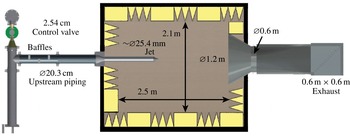
wedge-tip-to-wedge-tip anechoic chamber shown schematically in figure 3. The cloth covered fibreglass wedges (Eckel Industries) have a low-frequency cutoff of 250 Hz, as tested in accordance with the Impedance Tube Method-ASTM-C 384-90. Above this frequency they are reported to absorb 99 % of the incident energy. Due to the location of the microphones with respect to the wedges the actual cutoff is closer to 400 Hz (ISO 3745 2003), which is still below the range of interest in this paper.
Anechoic facility overview.

Air for the jet is supplied from pressurised tanks (
 $140~\text{m}^{3}$
of air at 890 kPa). To minimise upstream sound sources, large 20.3 cm piping is used between the tanks and the control valve (2.54 cm Fisher 667-ET-DVC6010 Globe Valve Assembly), which was operated with a PID control scheme in LabVIEW to maintain flow rate within
 $\pm 0.005$
of the target test Mach number.
To provide make-up air into the chamber, its upstream wall has two open sections based upon the design of similar facilities (Kerechanin Reference Kerechanin2000). These openings span the full height of the chamber, 2.1 m, and are 0.28 m wide. The velocity of the entrainment flow is about
 $3.5~\text{m}~\text{s}^{-1}$
for a
 $M=0.9$
jet, which is only about one-hundredth the velocity of the jet, and the flow is filtered as it enters the chamber by an aluminium 1 mm woven-wire screen mesh. Overhangs outside the chamber cut off the direct line of sound propagation into the chamber and are covered with a 2.54 cm thick acoustic absorbing polyurethane foam lining.
The jet exhaust is directed into a conical 1.2 m diameter bell mouth that blends smoothly into a
 $0.6~\text{m}\times 0.6~\text{m}$
duct. The exhaust ducting is made of acoustically absorbing perforated metal, and large-scale flow separation is avoided by using aerodynamic turning vanes. The entire exhaust collector was lined with polyurethane foam material to suppress reflected acoustic contamination of jet noise spectra, particularly at low frequencies (Viswanathan Reference Viswanathan2006). After the control valve (see figure 3), the 20.3 cm piping is also lined with polyurethane foam. Additionally, three baffles made from acoustical foam (Sonex One) were inserted in the upstream section to block any direct line of propagation from upstream to the jet exit. These were motivated by reported successful designs (Ahuja Reference Ahuja2003). Their spacing was set to be incompatible with the long-wavelength standing modes of the pipes. Before the nozzle, the flow was conditioned with a 2.54 cm thick piece of honeycomb (3.18 mm cell size) positioned downstream of the baffles backed by an aluminium screen (1.02 mm) (Pope & Harper Reference Pope and Harper1966). These are followed by a 20.3–10.2 cm contraction in the pipe diameter (figure 3).
2.2. Sound measurement
Brüel and Kjær type 4939 0.635 cm free-field microphones were oriented normal to the primary sound propagation direction with their protective gridcaps removed. These microphones are designed for intense and high-frequency measurements with a nearly uniform frequency response up to 100 kHz and a measurement uncertainty specification for our conditions of
 $\pm$
0.3 dB. They were positioned at 15° increments between
 ${\it\alpha}=90^{\circ }$
(sideline) and
 ${\it\alpha}=30^{\circ }$
(downstream) with the results from the intermediate angles reported elsewhere (Fontaine Reference Fontaine2014). All were greater than 35 jet diameters away from the jet exit, per the recommendation of Viswanathan (Reference Viswanathan2006). Sound pressures were sampled at 200 kHz and acquired for five seconds using LabVIEW software and collected into 93.6 Hz bins or, in some cases, into third-octave intervals per the ANSI S1 11-2004 (2004) standard. In this paper, SPL is reported in decibels (dB) with the usual reference pressure
 $p_{o}=2\times 10^{-5}~\text{Pa}$
. Following common practice, acoustic data are presented in lossless form with atmospheric absorption effects removed per ANSI S1 26-1995 (1995). A standard spherical divergence is assumed to compare measurements at different distances. Microphone uncertainty along with uncertainty associated with atmospheric conditions, length measurements, facility performance, and jet exhaust velocity produce a total sound level uncertainty of less than
 $\pm 0.5~\text{dB}$
for a typical measurement (Fontaine Reference Fontaine2014).
2.3. Facility validation
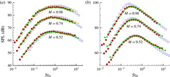
For validation, jet noise measurements are compared with accepted experimental data (Viswanathan Reference Viswanathan2004; Brown & Bridges Reference Brown and Bridges2006) in figure 4. The data are in excellent agreement, except perhaps for Mach 0.98 measurements taken at
 ${\it\alpha}=30^{\circ }$
, which are off by 2 dB, possibly due to transonic effects. Also shown is a comparison between a
 $D=2.68~\text{cm}$
copper nozzle and a
 $D=1.90~\text{cm}$
rapid prototyped nozzle (Selective Laser Sintering, PA 2200). Further discussion of these validations is available elsewhere (Fontaine et al.
Reference Fontaine, Bobbitt, Austin, Elliott and Freund2012; Fontaine Reference Fontaine2014) including tests confirming the anechoic properties of the chamber as well as confirmation that measured jet noise conforms to theoretical scalings.
Typical
 $1/3$
octave far-field sound spectra corrected to lossless conditions at
 $72D$
: ▪,
 $D=19~\text{mm}$
rapid prototyped nozzle; ▴,
 $D=26.9~\text{mm}$
machined metal nozzle; ▫, Brown & Bridges (Reference Brown and Bridges2006); and ▵, Viswanathan (Reference Viswanathan2004). (a) Sideline 90°; (b) downstream 30°.

2.4. Particle image velocimetry (PIV)
An essential component of our study is the measurement of turbulence statistics just downstream of the nozzle exits. For this, we used a two-component particle image velocimetry (PIV) system and a PCO camera, which provided a
 ${\sim}100~\text{pixels}~\text{mm}^{-1}$
maximum resolution. A New Wave Gemini dual-head Nd:YAG laser operating at
 $90~\text{mJ}/\text{pulse}$
at 532 nm creates the light sheet. By utilising a laser power meter, a translation stage, and a knife edge, the full-width-half-maximum thickness of the laser sheet was measured to be 0.19 mm. For all PIV experiments, the core flow is seeded with bis(2-ethylhexyl) sebacate (DEHS) using a Laskin nozzle designed to make
 $1~{\rm\mu}\text{m}$
particles (Humphreys & Bartram Reference Humphreys and Bartram2001). The entrained air is seeded with a Vicount 1300/180/2.2 kW smoke generator that produces
 $0.2~{\rm\mu}\text{m}$
median diameter particles (Concept Engineering Ltd 2011). All PIV equipment was removed from the chamber when making sound measurements.
Most turbulence statistics we report were based upon PIV images extending from
 $0.04D$
(
 ${\sim}1~\text{mm}$
) to approximately
 $3.5D$
(
 ${\sim}90~\text{mm}$
) downstream. Reported results use more than 1000 image pairs processed using the DaVis 8.1 software package from LaVision. Processing began with a
 $64~\text{pixel}\times 64~\text{pixel}$
interrogation zone to generate bulk motion estimates with resulting vector fields applied to
 $32~\text{pixel}\times 32~\text{pixel}$
interrogation windows with 50 % overlap. Cross-correlations between the image pairs were repeated three times at each interrogation site with the previous result used as an initial guess for the particle motion until velocity field results converged. A 4:1 elliptical interrogation zone with 75 % overlap using
 $32~\text{pixel}\times 32~\text{pixel}$
produced indistinguishable results. As a result, all analysis of the data presented in this paper was post-processed with a square
 $32~\text{pixel}\times 32~\text{pixel}$
interrogation zone.
Following the analysis of Lazar et al. (Reference Lazar, DeBlauw, Glumac, Dutton and Elliott2010), equipment uncertainty was found to yield only
 $\pm 2.5~\text{m}~\text{s}^{-1}$
uncertainty in the core of the jet, and the maximum particle lag as estimated from a Stokes drag is at most
 $1.7~\text{m}~\text{s}^{-1}$
. These uncertainties are well below those necessary to support the conclusions of this paper. Further details of the PIV system as well as additional details regarding these estimates are reported elsewhere (Fontaine Reference Fontaine2014).
2.5. Nozzles
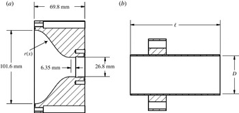
The nozzles in figure 5 were specifically designed to tailor the boundary layer thickness at the nozzle lip. All three nozzles use the same fifth-order polynomial contraction from the 10.2 cm diameter piping down to a straight length of copper tube with inner diameter
 $D=26.8~\text{mm}$
and wall thickness of 0.9 mm. The contraction is designed to have zero slope and zero curvature at both the beginning and end (Reshotko, Saric & Nagib Reference Reshotko, Saric and Nagib1997). The straight-walled nozzles thus differed only in their length
 $\ell$
, ranging from 63.5 to 508 mm. By using the same contraction, the state of the boundary layer at the beginning of each straight section will be the same, so the principal difference will be the length of the boundary layer development, which is quantified in § 3. There is no expectation that any will provide a fully developed pipe flow, such as considered by Sandberg et al. (Reference Sandberg, Sandham and Suponitsky2012).
(a) Schematic of contraction shape:
 $r(x)=D/2+(D_{u}/2-D/2)$
 $[10((L-x)/L)^{3}-15((L-x)/L)^{4}+6((L-x)/L)^{5}]$
, where
 $D_{u}=101.6~\text{mm}$
is the inlet diameter and
 $L=50.8~\text{mm}$
is the length of the contraction. (b) Schematic of the
 $D=26.8~\text{mm}$
family of straight-walled nozzles, with the short
 $\ell =63.5~\text{mm}$
nozzle shown. The medium
 $\ell =292.1~\text{mm}$
and long
 $\ell =508~\text{mm}$
nozzles are not shown.

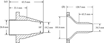
For comparison, two other nozzles, shown in figure 6, were also tested. These were manufactured using a Forminga P 100 selective laser sintering (SLS) system. The first has a
 $D=19.2~\text{mm}$
exit and contracts linearly without a straight section. The second has a larger exit diameter of
 $D=34.5~\text{mm}$
, which approximately doubles the mass flow rate. As with the
 $D=26.8~\text{mm}$
straight-walled nozzles it has a fifth-order polynomial contraction followed by a straight section. These nozzles were included to the support relative insensitivity of our results to how the turbulent boundary layer forms in our three primary nozzles, which is considered in detail in § 4.
Schematics of (a) the small- and (b) large-diameter alternative configuration nozzles. Nozzle (a) is inserted into the contraction in figure 5(a) and nozzle (b) has a contraction that follows a similar polynomial reduction.

3. Turbulence statistics
3.1. Momentum thickness and near-nozzle spreading
We are particularly interested in the very near-nozzle shear-layer thickness and its growth. This is quantified with the momentum thickness,
 $$\begin{eqnarray}{\it\theta}(x)=\int _{r_{05}}^{r_{95}}\frac{U(x,r)}{U_{j}}\left(1-\frac{U(x,r)}{U_{j}}\right)\!\text{d}r,\end{eqnarray}$$
where
 $U$
is the time-averaged streamwise velocity and
 $U_{j}=U(x=0,r=0)$
is its mean on the jet centreline at the exit. The integration bounds correspond to the 5 % points (
 $0.05U_{j}$
and
 $0.95U_{j}$
) in the mean velocity profile. Alternative integration bounds corresponding to
 $0.02U_{j}$
and
 $0.98U_{j}$
produced indistinguishable results. The effect of including the mean density in (3.1) was estimated using the Crocco–Busemann relationship. This was found to change the momentum thickness only slightly (
 ${\lesssim}10\,\%$
), though with essentially the same effect for all the jets since they share a common temperature ratio. None of the conclusions would depend upon this, nor would they be expected to change for other measures of thickness because they so closely track each other, even in approximately self-similar free shear flows (e.g. Freund, Moin & Lele Reference Freund, Moin and Lele1997). The downstream spreading of
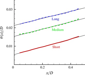
 ${\it\theta}$
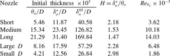
is linear, as shown in figure 7. A key length scale is its thickness right at the nozzle lip, which we estimate by linear extrapolation to
 $x=0$
. These values are tabulated in table 1. The
 ${\it\theta}=0.005D$
value we find for the short nozzle is similar to other reported values:
 ${\it\theta}/D=0.0036$
(Viswanathan & Clark Reference Viswanathan and Clark2004),
 ${\it\theta}/D=0.002$
(Zaman Reference Zaman1985b
),
 ${\it\theta}/D=0.005$
(Husain & Hussain Reference Husain and Hussain1979), and
 ${\it\theta}/D=0.002$
(Samimy et al.
Reference Samimy, Kim, Kastner, Adamovich and Utkin2007).
Measured momentum thickness for the short, medium and long nozzles, and the linear fits used to extrapolate to nominal nozzle values.


3.2. Turbulence development
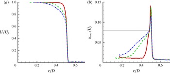
Profiles of the streamwise mean flow and turbulence intensity are shown at
 $x=0.04D$
in figure 8. We see thicker shear layers for the longer nozzle. However, shear-layer mean profiles do not simply rescale with
 ${\it\theta}_{o}$
or any single length scale, as seen also by their different shape factors
 $H$
(table 1). This gives them a distinct character from a fully developed free shear flow. The streamwise turbulence intensity in figure 8(b) is likewise complex. It seems to show two distinct regions, one presumably a remnant of the boundary layer profile and the other associated with the inflectional instability of the free shear profile. The apparent boundary layer remnant has a relatively shallow rise and reaches a streamwise turbulence intensity of about
 $0.08U_{j}$
. This region is markedly sensitive to the boundary layer thickness and is much more pronounced at the same downstream location for the longer nozzles. The second region has a sharply peaked turbulence intensity. Despite the factor of 3.9 variation in momentum thickness, this sharply peaked region is approximately the same for all nozzles. The peak intensity ranges only from
 $u_{rms}=0.12U_{j}$
for the long-nozzle case up to
 $0.14U_{j}$
for the short-nozzle case. This two-region structure is similar to measurements reported by Morris & Foss (Reference Morris and Foss2003) for an effectively incompressible plane boundary layer leaving a sharp corner and forming a free single-stream planar shear layer with
 $\mathit{Re}_{{\it\theta}}=4560$
.
Streamwise velocity statistics at
 $x=0.04D$
: ——, short; - - - -, medium; – - – - –, long nozzles. (a) Mean velocity. (b) Turbulence intensity; the horizontal line at
 $u_{rms}/U_{j}=0.08$
is for reference.

3.3. Nozzle-lip thickness
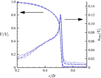
For any such flow there is a possibility that turbulence near the nozzle is sensitive to the thickness of the nozzle lip, though this is more of a concern if the boundary layer leaving the nozzle is laminar. Here we empirically confirm insensitivity to the nozzle-lip thickness and in the following section demonstrate that the turbulence is well-established at the nozzle exit by several measures in addition to the intensity shown in figure 8(b).
Nozzle-lip thickness was varied by attaching a 12.7 mm long sharpened plastic extension ring to the long nozzle. Changing from the baseline lip thickness of
 $0.0332D$
to
 $0.0172D$
and
 $0.0093D$
, the thinnest of which could not be measured precisely, had no obvious influence on the mean or turbulence statistics at
 $x=0.04D$
, as seen in figure 9.
Mean flow and streamwise turbulence intensity for different nozzle-lip thicknesses: – - – - –,
 $d=0.0332D$
; – - - – - -,
 $d=0.0172D$
;
 $\cdots \cdots$
,
 $d\lesssim 0.0093D$
.

3.4. Nozzle boundary layer turbulence
As discussed in § 1, the initial boundary layer can play an important role in the noise generated by a jet. Unfortunately, it is difficult to quantify the initial turbulence state from nozzle profiles and shape factors alone (table 1) so we also consider several other metrics. Brown & Bridges (Reference Brown and Bridges2006) identified a particular hump-shaped feature in the far-field spectra from nozzles thought to have a laminar exit flow condition. The spectra we measure, as we shall see in figure 15, show no corresponding feature, supporting a turbulent condition at the nozzle. We also consider several more direct measures that indicate a turbulent nozzle boundary layer.
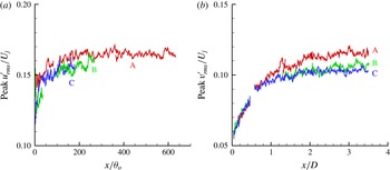
In addition to the linear spreading (figure 7), the peak streamwise turbulence intensity is nearly uniform (figure 10
a). It is not expected to be exactly uniform downstream, since flow is not expected to be fully developed into a self-similar state this close to the nozzle, but obvious features consistent with laminar flow (Husain & Hussain Reference Husain and Hussain1979) are not seen. The peak turbulence intensity is consistent with turbulence intensity values at all points we measure in
 $x$
(Husain & Hussain Reference Husain and Hussain1979; Zaman Reference Zaman1986); the peak radial turbulence intensity (figure 10
b) develops more slowly than the streamwise fluctuation, but is likewise consistent with free-shear-flow turbulence.
Downstream evolution of the peak (a) streamwise and (b) radial turbulence intensity for the short (A), medium (B) and long (C) nozzles.

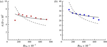
If the shear layers are turbulent, they should also be relatively insensitive to the Reynolds number. This is quantified in figure 11, which shows the
 ${\it\theta}_{o}$
variation when Reynolds number is changed by a factor of 6. Despite a potentially weak Mach-number dependence because it was not possible to do this without also changing Mach number from
 $M=0.2$
to 0.9, we found a
 ${\it\theta}$
dependence that is consistent with a turbulent flow. It is much better fitted by the empirical
 $\mathit{Re}_{D}^{1/7}$
, often seen for turbulence, than the
 $\mathit{Re}_{D}^{1/2}$
scaling for laminar flow. A similar metric was used to support a turbulent nozzle condition by Zaman (Reference Zaman2012).
Nozzle momentum thickness sensitivity to
 $\mathit{Re}_{D}$
with anticipated turbulent
 $\propto \mathit{Re}^{1/7}$
(——) and laminar
 $\propto \mathit{Re}^{1/2}$
(- - - -) fits. (a) Short (⬦) and (b) long (●) nozzle.

If it can be measured actually in the boundary layer, the shape factor
 $H$
can also be used to assess the flow condition. It might, therefore, be a concern that
 $H$
for the short nozzle,
 $H=2.18$
, is somewhat closer to a nominal laminar boundary layer value of
 $H=2.6$
than are the corresponding values for the longer nozzles (
 $H\approx 1.5$
), which is closer to the nominal turbulence boundary layer
 $H=1.4$
(see table 1). However, it is important to recognise that at this first measurement location the flow is not an equilibrium boundary layer. Indeed, the turbulence intensity profiles at the first measurement location show that the flow in all cases has already evolved significantly away from a boundary layer profile for which a shape factor metric would provide a better indication of flow regime (figure 8
b). It should also be noted that the shorter nozzle, with its thinner boundary layer, has evolved for
 $x=1.8{\it\theta}_{o}$
, whereas the medium-length nozzle only for
 $x=0.65{\it\theta}_{o}$
, so it should indeed retain less of a boundary layer character at the first measurement location.
The rapid approach to apparent self-similar behaviour we see in figures 10 and 12 similarly supports a turbulent nozzle flow condition. Shear layers that originate from a separating laminar boundary layer require
 $1000{\it\theta}_{o}$
to become self-similar (Bradshaw Reference Bradshaw1966) whereas those from turbulent boundary layers achieve approximate self-similarity in less than
 $150{\it\theta}_{o}$
(Hussain & Zaman Reference Hussain and Zaman1985), with Morris & Foss (Reference Morris and Foss2003) finding
 $x>100{\it\theta}_{o}$
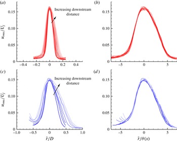
sufficient for a similarity scaling to collapse the mean streamwise velocity profiles. Figure 12 shows that the present turbulence intensity indeed collapses versus
 $r/{\it\theta}(x)$
for
 $x\gtrsim 100{\it\theta}_{o}$
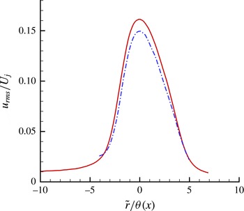
. This collapse is nearly the same for both the long and short nozzles as shown in figure 13.
Downstream streamwise fluctuations versus
 $\tilde{r}=r-D/2$
subject to different scaling factors: (a,c)
 $D$
scaling; (b,d)
 ${\it\theta}$
scaling. The plot lines are lighter in tone for larger
 $x$
in the downstream direction: (a,b) the short-nozzle data equally spaced from
 $107{\it\theta}_{o}$
to
 $240{\it\theta}_{o}$
; and (c,d) the long-nozzle data equally spaced from
 $110{\it\theta}_{o}$
to
 $230{\it\theta}_{o}$
.

Mean downstream (approximately self-similar region) streamwise fluctuation profiles for the short (——) and long (– - – - –) nozzles.

3.5. Near-nozzle shear-layer development
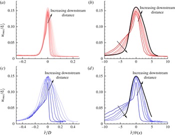
The downstream development of the turbulence in figure 14 shows how the features noted in regard to figure 8(b), which seem to be a persisting remnant of the nozzle boundary layers, disappear as the flow develops towards free-shear-flow behaviour. The intermediate-length nozzle shows an analogous behaviour (Fontaine Reference Fontaine2014).
As figure 12 but for near-nozzle streamwise turbulence intensity from
 $x=0$
to
 $100{\it\theta}_{o}$
: (a,b) the short nozzle with equally spaced profiles from
 $x=9{\it\theta}_{o}$
to
 $84{\it\theta}_{o}$
; and (c,d) the long nozzle with equally spaced profiles from
 $x=5{\it\theta}_{o}$
to
 $95{\it\theta}_{o}$
.

When the radial coordinate is normalised by
 $D$
we see the relative persistence of the turbulence intensity into the core flow, especially for the thick boundary layer of the long nozzle in figure 14(c). This is presumably a remnant of the boundary layer turbulence from the nozzle. This portion of the profile appears to be enveloped by the spreading of the peak turbulence, which at about this same
 $x$
-location shows a similarity collapse (figure 14). This is especially evident for the long-nozzle case in figure 14(c). The short nozzle shows the same basic behaviour, though the boundary layer footprint is, of course, much smaller relative to the diameter.
Since the mean flow profile drives turbulence production, it is somewhat surprising that despite the obvious difference in the mean flow profile in this region, the peak turbulence seems to develop nearly the same. We investigate this in more detail in § 5, where linear instability analysis suggests that instabilities are indeed insensitive to the boundary layer remnant of the nozzle flow.
3.6. Potential core length
For purposes of comparison, the potential core length
 $L_{c}$
is defined by the
 $U(L_{c},0)=0.95U_{j}$
point on the jet axis. With this definition, the long-nozzle potential core
 $L_{c}=7.90D$
is
 $0.77D$
shorter than the short-nozzle case,
 $L_{c}=7.13D$
. Full PIV results are reported elsewhere (Fontaine Reference Fontaine2014). This is approximately the same as the reduction we should anticipate based on simple geometric reasoning following figure 1. The
 ${\it\theta}_{o}$
for the long-nozzle case matches the short-nozzle case at
 $x=0.72D$
, which is close to the
 $0.77D$
reduction in potential core length. This supports a relatively close relationship between these two jets once the short-nozzle mixing layer spreads to match the long-nozzle thickness at its nozzle.
4. Far-field sound
4.1. Nozzle comparison
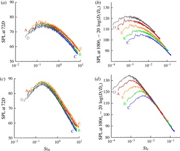
The different near-nozzle behaviours lead to the clear differences in the far-field sound spectra seen in figure 15. At high frequencies, the long nozzle, with its 3.9 times thicker initial shear layer, generated 3 dB less intense downstream (
 ${\it\alpha}=30^{\circ }$
) sound. The nominally missing thin shear-layer region for the thicker boundary layer jets should radiate high-frequency sound because of its smaller
 ${\sim}{\it\delta}$
locally largest turbulence. So we can speculate that portions of the far-field high-frequency spectra might collapse with the initial shear-layer thickness. This is supported by the success of
 $\mathit{St}_{{\it\theta}}=f{\it\theta}_{o}/U$
at collapsing the high-frequency part of the spectra in figure 15(d), which also includes the alternative nozzles from figure 6. This suggests that this portion of spectrum is indeed related to the
 ${\it\delta}$
-scale, specifically the
 ${\it\theta}_{o}$
-scale near-nozzle shear layer.
(a,b) Sideline (
 ${\it\alpha}=90^{\circ }$
) and (c,d) downstream (
 ${\it\alpha}=30^{\circ }$
) noise measurements for the short (A), medium (B), long (C), small-
 $D$
(D) and large-
 $D$
(E) nozzles: (a,c)
 $D$
scaling; (b,d)
 ${\it\theta}_{o}$
scaling.

However, this simple scaling with
 ${\it\theta}_{o}$
is not successful for
 ${\it\alpha}=90^{\circ }$
, even when the spectra are extrapolated, such as with the empirical spectra of Tam et al. (Reference Tam, Golebiowski and Seiner1996). Figure 15(a,b) shows these sideline spectra. This lack of
 ${\it\theta}_{o}$
-based collapse is consistent with the tacit expectation that at 90° the measured sound is made up of contributions from the relatively random turbulence throughout the jet. These ideas are consistent with the role of mean shear in early aeroacoustic theories (Ribner Reference Ribner1969), wave-like eddy models of noise (Mankbadi & Liu Reference Mankbadi and Liu1984), and motivate some empirical noise source modelling (Tam & Auriault Reference Tam and Auriault1999). Because this nominally missing portion of shear-layer growth represents a small fraction of the total volume of turbulent flow, we do not expect changes to be so apparent in the sideline sound spectra. The same behaviour is observed at
 $M_{j}=0.7$
(Fontaine Reference Fontaine2014). The acoustic radiation from the other two nozzles considered, which were not in the same long–medium–short family, similarly collapse when scaled accordingly (figure 15). For these other nozzles, we subtracted the usual
 $20\log (D/D_{o})$
to account for the difference in nozzle size, with
 $D_{o}=26.8~\text{mm}$
, the size of the nozzles in the baseline study.
4.2. Noise reduction
We note that one effect of a thicker boundary layer is to reduce noise. Most simply, a thick exhaust boundary layer removes the initial region of shear-layer growth up to the point where the shear-layer thickness are equivalent. The total acoustic power is reduced with this region now missing, and the potential core closes earlier. There is a smaller noise generation volume, especially that which is associated with shear-layer instabilities and radiates predominantly downstream (Jordan & Colonius Reference Jordan and Colonius2013). Since this is the small
 ${\it\delta}$
-scale region near the nozzle exit, it is primarily high-frequency noise that is removed by this effect, which is shown in our spectra, figure 15.
The nozzle boundary layer thickness is closely related to many control devices that have been implemented in an attempt to reduce noise, with one of the most popular being chevrons. The exhausting shear layer is altered from the baseline; however, the mechanism by which noise reductions arise is likely to be different to that for the thicker shear-layer exhaust. While a precise understanding is still lacking because it is tied up in the full complexity of jet turbulence, chevrons are believed to disrupt the coherence of large-scale azimuthally correlated vortex-like structures (Alkislar, Krothapalli & Lourenco Reference Alkislar, Krothapalli and Lourenco2005), which thereby have their vorticity redistributed into streamwise-oriented vortex structures. Michalke & Fuchs (Reference Michalke and Fuchs1975) suggest that the lowest-order azimuthal modes constitute the most important sound sources, which was supported by the experiments of Juvé, Sunyach & Comte-Bellot (Reference Juvé, Sunyach and Comte-Bellot1979) who measured their signatures in the acoustic far field. The result is decreased sound near the peak Strouhal number and below (
 $\mathit{St}_{D}\lesssim 1$
) (Bridges & Brown Reference Bridges and Brown2004). At higher frequencies, however, the streamwise vortex pairs can increase overall turbulence intensity, thereby increasing high-frequency mixing noise. The chevrons can be designed in such a way as to minimise the high-frequency penalty or attempt to push it to frequencies outside of the audible range; however, eliminating it completely remains challenging (Bridges & Brown Reference Bridges and Brown2004).
The spectra in figure 15 show that sound is also reduced at low
 $\mathit{St}_{D}$
for the thicker-shear-layer longer-nozzle cases. As with many features of subsonic jet noise, the precise mechanism is unclear. However, this is consistent with reported results for the effects of chevrons. Bridges & Brown (Reference Bridges and Brown2004) also show that deeper chevron penetration through the boundary layer can lead to larger noise reductions at low frequency. This presumably alters the downstream dynamics sufficiently to suppress the generation of some low-frequency sound. However, chevrons in this case can also increase sound at higher frequencies, presumably radiated directly from near the nozzle where they most disturb the flow. There is no such development in the present case with its relatively undisturbed, though thicker, turbulent boundary layer. The present results show that without chevrons there is a comparable direct effect of the boundary layer thickness, and the interplay of chevrons with the turbulent boundary layer thickness has not been studied in detail, though our results suggest that adjusting this might provide additional tailoring of any related noise-control approach. A designer would need to balance sound reduction against losses associated with the formation of a thicker turbulent boundary layer, but it is also possible that this could be done with trips introduced in an on-demand basis.
5. Linear stability
Figure 14 shows that part of the turbulence intensity profile downstream evolution is remarkably insensitive to the significantly different mean flow profiles of figure 8. Superficially, the only difference is that more downstream development is required before the apparently more active region of turbulence envelopes the remnants of the thicker boundary layer (particularly, figure 14
c). This narrow peak shows an apparent
 ${\it\delta}$
-scaling collapse well before it subsumes the smaller-
 $r$
boundary layer remnant, which suggests that the self-sustaining mechanisms of the turbulence here are approximately independent of the mean velocity profile differences.
To support this relative insensitivity, we consider the linear stability of the measured mean velocity profiles. Though linear analysis can usually at most provide a phenomenological model of the root mechanisms of turbulence, stability analysis has been remarkably effective in anticipating mixing layer growth rates (Gropengeisser Reference Gropengeisser1970; Sandham & Reynolds Reference Sandham and Reynolds1990; Viswanathan & Morris Reference Viswanathan and Morris1992), the well-known spanwise-oriented rollers that resemble Kelvin–Helmholtz modes (Brown & Roshko Reference Brown and Roshko1974; Roshko Reference Roshko, Bodner, Singer, Golan and Hashin1993), the response of forced mixing layers (Gaster, Kit & Wygnanski Reference Gaster, Kit and Wygnanski1985; Cohen & Wygnanski Reference Cohen and Wygnanski1987), and particular components of supersonic jet noise (Tam & Burton Reference Tam and Burton1984).
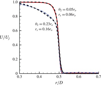
For specificity and to avoid any small amounts of measurement noise and variability in the experimental data, analytic functions with well-behaved derivatives are fitted to the measured profiles, as shown in figure 16. A single hyperbolic tangent profile, which has provided an obvious choice for stability analysis in many cases, was found to be inadequate because of the unusual near-nozzle profile shapes. Fortunately, the product
 $$\begin{eqnarray}\displaystyle \frac{U}{U_{j}}=0.5\left[1-\tanh \left(\frac{r_{o}}{4{\it\theta}_{1}}\left[\frac{r}{r_{o}}-\frac{r_{o}}{r}\right]\right)\right]0.5\left[1-\tanh \left(\frac{r_{o}}{4{\it\theta}_{2}}\left[\frac{r-r_{s}}{r_{o}}-\frac{r_{o}}{r-r_{s}}\right]\right)\right]\qquad & & \displaystyle\end{eqnarray}$$
fits the data well: one factor represents the higher-shear region separating the jet from the quiescent ambient flow and the other, once it is offset from
 $r=D/2$
, represents the lower-shear inner boundary layer remnant. Taking
 ${\it\theta}_{1}=0.0109r_{o}$
and
 $r_{o}=0.5$
provides a common fit for both cases. For the short and long nozzles, other fitting parameters were
 ${\it\theta}_{2}=0.05r_{o}$
and
 $r_{s}=0.06r_{o}$
, and
 ${\it\theta}_{2}=0.23r_{o}$
and
 $r_{s}=0.16r_{o}$
, respectively. For reference we also consider a baseline configuration with only the first factor from (5.1).
Mean velocity for the short (——) and long (– - – - –) nozzles, and corresponding fits using (5.1) (- - - -).

These velocity profiles, along with density,
 $\bar{{\it\rho}}$
, determined from the Crocco–Buseman relationship, are supplied to a linear stability code modified from Kim et al. (Reference Kim, Bodony and Freund2014). A standard formulation with a shooting method is used. Full details are reported elsewhere (Fontaine Reference Fontaine2014).
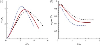
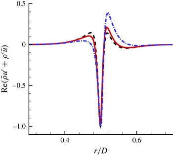
The instability amplification rates and phase speeds for the baseline profile and the short- and long-nozzle profiles are shown in figure 17. The peak amplification rates are indeed only weakly dependent upon the large difference in momentum thickness for these profiles. It is clear that the instability is primarily driven by the high-shear portion of the profile, with only minor differences due to the thick boundary layer remnant. The eigenfunctions are somewhat different, as seen in figure 18, though they have the same general shapes and radial extent. Only the first axisymmetric mode
 $n=0$
is shown since it is the most amplified; however, other modes have similar behaviour (Fontaine Reference Fontaine2014). While no linear model will completely describe the inherently nonlinear mechanisms of a turbulent shear layer, it is apparent that linear mechanisms support similar development to that apparent in the measured turbulence statistics.
(a) Axisymmetric mode
 $n=0$
amplification and (b) phase speed for
 $\text{e}^{\text{i}{\it\alpha}x+\text{i}{\it\omega}t}$
modes with
 ${\it\alpha}={\it\alpha}_{r}+\text{i}{\it\alpha}_{i}$
: - - - -, baseline; ——, short nozzle; – - – - –, long nozzle.

The real part (
 $\text{Re}$
) of the streamwise momentum eigenfunction with
 $u^{\prime }$
and
 ${\it\rho}^{\prime }$
the streamwise velocity and density eigenvectors for baseflow velocity
 $\bar{u}$
and density
 $\bar{{\it\rho}}$
, respectively.

6. Conclusions and additional discussion
The family of nozzles we studied allowed a direct examination of the effect of turbulent boundary layer thickness. The turbulence state of the boundary layer, even at significantly lower Reynolds numbers, was established via several metrics, which is important given the widely recognised effects associated with laminar flow at the nozzle. Fluctuation statistics at
 $x=0.04D$
showed out-of-equilibrium turbulence, which is expected this close to the nozzle. The high-speed part of the shear layer appeared to be a remnant of the nozzle boundary layer, which was particularly pronounced in the thicker boundary layer cases. However, at the outer edge of the jet, the turbulence was approximately insensitive to the boundary layer thickness. Its intensity showed a narrow peak, which developed with an apparently self-similar character when scaled with the local momentum thickness despite the persistent retarded velocity associated with the thicker boundary layer remnants toward the core of the jet. This behaviour, which was unexpected given the difference in boundary layer thickness, is consistent with the relative insensitivity of the corresponding linear instabilities of these profiles, despite their significantly different thicknesses. The shear at the inflection point is associated with the outer edge of the flow and is nearly the same in all cases, which appears to be most important for the observed instability behaviour.
These different flows had an obvious effect on the far-field sound. The high-frequency downstream acoustic radiation scaled with the exit momentum thickness for all the nozzles considered. This might not be expected since the mean flows were fundamentally different in the thick and thin limits, with differences that are not well characterised by a single thickness length scale. However, as with turbulence statistics, this similarity of downstream radiation might be explained by the relatively similar instability modes they support. The peak spectrum was less affected by the nozzle shear-layer thickness, but also showed a reduced sound in the thicker shear layer cases.
No similar collapse of the acoustic data was found for the measurable portions of the spectrum at
 ${\it\alpha}=90^{\circ }$
. Though it is difficult to prove, this would be consistent with the often-voiced notion that the sideline sound is not associated with predominantly shear-layer-supported wavepacket-like structures, which radiate predominantly downstream. The better collapse with
 $D$
than
 ${\it\theta}_{o}$
at all frequencies is more consistent with a source that might correspond to smaller-scale turbulence distributed throughout the jet. Alternatively, the sideline noise could be generated via a different mechanism by the same structures in the flow (Goldstein & Leib Reference Goldstein and Leib2005). While this might be the case, if such a mechanism were responsible for a significant portion of the sideline noise, there would also be some systematic change in the sideline spectra, so we do not find strong support for this perspective.
Though further detailed studied is necessary for any specific conclusions to be drawn, we can discuss some of the implications of the present observation. The implication for numerical simulations of turbulent jet noise is that their often artificially thick nozzle shear layer might significantly affect the predicted far-field sound. However, the apparent collapse of key components of the spectrum, when scaled by the nozzle exit conditions likewise suggests the possibility of correction. Any such correction would also need to recognise that the shear layers in these experiments have a particular form, with an obvious remnant of a nozzle boundary layer and relatively steep portion in the neighbourhood of their inflection point. Any thick inflow shear layer in a simulation will not necessarily share this character, the full implications of which cannot be anticipated with our results. A smooth profile, such as a commonly used
 $\tanh$
-profile, would not necessarily be the best choice for modelling a nozzle exit flow without a nozzle. A thicker shear layer, such as we measure in our thick boundary layer case, might provide a better alternative, but the steep region of a profile, such as we measure, would not necessarily reduce the resolution challenge.
One obvious effect of thicker nozzle boundary layers is to reduce noise, which will have implications for both simulation-based predictions of noise suppression, with their often artificially thick shear layers, and engineering implementations. Chevrons, for example, require a particular arrangement and boundary layer penetration for them to reduce sound, and even then generally only at low frequencies. Generating a thicker nozzle-exit boundary layer, without incurring losses or generating noise, might offer a similarly successful approach to noise control, particularly at high frequency. This might be best accomplished with retractable passive actuators, which would not incur significant losses when retracted. Thick boundary layers might similarly affect active control. In terms of the responsiveness of the near-nozzle jet to actuation, the similar turbulence development and stability might allow scale experiments to examine at least some aspects of control strategies. However, their effect on the far-field sound might be masked by the same shear-layer-thickness sensitivity we report here.
Acknowledgements
We gratefully acknowledge support from Rolls-Royce and Gulfstream Aerospace Corporation and the Office of Naval Research (N00014-11-1-0756).