2. Problem description

In the present work, our concern is with an incompressible viscous fluid of kinematic viscosity $\nu$ in a pipe with elliptical cross-section ${x^2}/{a^2}+{y^2}/{b^2}=1$ for various values of aspect ratio $A=a/b$. Following Kerswell & Davey (Reference Kerswell and Davey1996), the Reynolds number, $Re$, is based on the speed of the base flow at $x=y=0$ and a length scale chosen as $\sqrt {(a^2+b^2)/2}$, so that the semi-major and semi-minor axes of the pipe measure $\sqrt {1+\beta }$ and $\sqrt {1-\beta }$ respectively, with $\beta =({A^2-1})/({A^2+1})$ for given aspect ratio $A$. We describe the problem in a non-orthogonal elliptical coordinate system where a point $(x,y)$ on the elliptical cross-section is defined by $x=\sqrt {1+\beta }\, r \cos \theta$ and $y=\sqrt {1-\beta }\, r \sin \theta$ for $0< r\le 1$ and $0 \le \theta < 2{\rm \pi}$.

We are looking for TW solutions of the Navier–Stokes equations for the perturbation velocity ${\boldsymbol v} (r, \theta , z-ct )=u\tilde {\boldsymbol r}+v\tilde {\boldsymbol {\theta }}+w\hat {\boldsymbol z}$ and pressure $p (r, \theta , z-ct )$, where

(2.1a,b)\begin{align} \tilde{\boldsymbol r}= \sqrt{1+\beta} \cos \theta\, \hat{\boldsymbol x}+ \sqrt{1-\beta}\sin \theta \, \hat{\boldsymbol y}, \quad \tilde{\boldsymbol{\theta}}={-} \sqrt{1+\beta}\sin \theta \, \hat{\boldsymbol x}+\sqrt{1-\beta}\cos \theta \, \hat{\boldsymbol y}, \end{align}

and $\hat {\boldsymbol z}$ is a unit vector in the axial direction. The pipe is aligned along the $z$-axis with the base flow ${\boldsymbol v}_B(r)= (1-r^2) \boldsymbol {\hat z}$. We assume ${\boldsymbol v} (r, \theta , z-ct )$ and $p (r, \theta , z-ct )$ to be $2{\rm \pi}$-periodic in $\theta$ and $\alpha (z-ct)$, and we assume that ${\boldsymbol v}$ satisfies a no-slip boundary condition on the wall. The TWs discussed here correspond to a constant mean axial pressure gradient $-4Re^{-1}\boldsymbol {\hat z}$, which drives ${\boldsymbol v}_B$ in the unperturbed case.

The non-dimensional Navier–Stokes equations become

(2.2)\begin{equation} -c{\boldsymbol v} + {\boldsymbol v} {\boldsymbol \cdot} {\boldsymbol \nabla} {\boldsymbol v}+ {\boldsymbol v}_B {\boldsymbol \cdot} {\boldsymbol \nabla} {\boldsymbol v}+ {\boldsymbol v} {\boldsymbol \cdot} {\boldsymbol \nabla} {\boldsymbol v}_B ={-} \boldsymbol{\nabla} p + \frac{1}{Re} \Delta {\boldsymbol v}, \quad {\boldsymbol \nabla} {\boldsymbol \cdot} {\boldsymbol v} = 0 , \end{equation}

where

(2.3a,b) \begin{align} ({\boldsymbol v} {\boldsymbol \cdot} {\boldsymbol \nabla}) {\boldsymbol v}=\begin{pmatrix} u\dfrac{\partial u}{\partial r}+ \dfrac{v}{r}\left( \dfrac{\partial u}{\partial \theta}-v\right)+w\dfrac{\partial u} {\partial z}\\ u\dfrac{\partial v}{\partial r}+ \dfrac{v}{r} \left( \dfrac{\partial v}{\partial \theta}+u\right)+w\dfrac{\partial v } {\partial z}\\ u\dfrac{\partial w}{\partial r}+ \dfrac{v}{r}\dfrac{\partial w}{\partial \theta}+w\dfrac{\partial w} {\partial z}\\ \end{pmatrix},\quad \boldsymbol{\nabla} p=\begin{pmatrix} F_{1}(\theta)\dfrac{\partial p}{\partial r} + \dfrac{1}{r}F_{3}(\theta)\dfrac{\partial p}{\partial \theta} \\ F_{3}(\theta)\dfrac{\partial p}{\partial r} + \dfrac{1}{r}F_{2}(\theta)\dfrac{\partial p}{\partial \theta}\\ \dfrac{\partial p}{\partial z} \end{pmatrix} \end{align}

and

(2.4) \begin{equation} \Delta {\boldsymbol v}= \begin{pmatrix} \left( \Delta_e - \dfrac{1}{r^2}F_{2}(\theta)\right)u-\left( \dfrac{2}{r}F_{3}(\theta)\dfrac{\partial v}{\partial r}+\dfrac{2}{r^2}F_{2}(\theta)\dfrac{\partial v}{\partial \theta}-\dfrac{2}{r^2}F_{3}(\theta)v\right)\\ \left( \Delta_e-\dfrac{1}{r^2}F_{2}(\theta)\right)v + \left(\dfrac{2}{r}F_{3}(\theta)\dfrac{u}{\partial r} +2 \dfrac{1}{r^2}F_{2}(\theta)\dfrac{\partial u}{\partial \theta}- \dfrac{2}{r^2}F_{3}(\theta)u \right)\\ \Delta_e w \end{pmatrix}, \end{equation}

with

(2.5)\begin{equation} \Delta_e = F_{1}(\theta)\frac{\partial^2}{\partial r^2}+ \frac{1}{r}F_{2}(\theta)\frac{\partial}{\partial r}+ \frac{2}{r}F_{3}(\theta)\frac{\partial^2}{\partial r \partial \theta} +\frac{1}{r^2}F_{2}(\theta)\frac{\partial^2}{\partial \theta^2}- \frac{2}{r^2}F_{3}(\theta)\frac{\partial}{\partial \theta}+\frac{\partial^2 }{\partial z^2} \end{equation}

and

(2.6a–c)\begin{equation} F_{1}(\theta)=\frac{1-\beta \cos (2 \theta)}{1-\beta^2},\quad F_{2}(\theta)=\frac{1+ \beta \cos (2 \theta)}{1-\beta^2} , \quad F_{3}(\theta)=\frac{\beta \sin (2 \theta)}{1-\beta^2}. \end{equation}

The continuity equation takes the form

(2.7)\begin{equation} \frac{\partial u }{\partial r} + \frac{u}{r} +\frac{1}{r}\frac{\partial v }{\partial \theta} +\frac{\partial w}{\partial z}=0. \end{equation}

This coordinate system reduces to cylindrical polar coordinates when $\beta =0$, making it a convenient choice for numerical continuation methods. Solutions to (2.2) have been computed in Ozcakir et al. (Reference Ozcakir, Tanveer, Hall and Overman2016) and others for a pipe with circular cross-section. Our procedure is to use these TWs for an initial guess in the Newton iteration procedure for TW solutions to determine TW states with higher aspect ratios. The TWs computed by Ozcakir et al. (Reference Ozcakir, Tanveer, Hall and Overman2016) possess a number of important symmetries in a pipe of circular cross section and are defined as

(2.8a)\begin{align} (k_0\text{-fold rotation}) \quad \mathbb{R}_{k_{0}} :( u,v,w,p) (r,\theta,z) \rightarrow (u,v,w,p)(r,\theta + 2{\rm \pi}/k_{0},z), \end{align}

(2.8b)\begin{align} (\text{shift-and-reflect}) \quad \mathbb{S}:( u,v,w,p) (r,\theta,z)\rightarrow (u,-v,w,p)(r,-\theta,z+{\rm \pi}/\alpha), \end{align}

(2.8c)\begin{align} (\text{shift-and-rotate})\quad \varOmega_{k_0} : ( u,v,w,p) (r,\theta,z) \rightarrow (u,v,w,p)(r, \theta+{\rm \pi}/k_0 ,z+{\rm \pi}/\alpha), \end{align}

where $k_0$, $\alpha$ are the azimuthal and axial wavenumbers, respectively. For the flow in an elliptical pipe, we retain the $\mathbb {S}$ symmetry, i.e. the azimuthal phase is fixed. The $\mathbb {R}_{k_{0}}$ symmetry is relevant only for $k_0=1,2$, because of the ${\rm \pi}$-radian rotational symmetry of the ellipse. Also, the $\varOmega _{k_0}$ symmetry is broken when $k_0=2$, because of terms proportional to $\cos 2\theta$ and $\sin 2\theta$ appearing in the equations of motion. Therefore, in our calculations we will only consider TWs with $\mathbb {S}$ symmetry in combination with $\mathbb {R}_{1}, \mathbb {R}_{2}$ and $\varOmega _{1}$ symmetries. It should be noted that when $k_0=1$, the $\varOmega _{1}$ symmetry together with $\mathbb {S}$ symmetry imply mirror symmetry about the $\theta ={\rm \pi} /2$ plane, i.e. the $y$-axis on the $xy$-plane which corresponds to top–bottom symmetry when the pipe is rotated ${\rm \pi} /2$ radians around its axis for $A<1$.

Our computational method is based on a Galerkin truncation of the Fourier modes in $\theta$ and $\tilde {z}=z-ct$ and a Chebyshev representation in $r$ which automatically accounts for the boundary condition; see Ozcakir et al. (Reference Ozcakir, Tanveer, Hall and Overman2016) for details. We use the following truncated basis representation for the velocity ${\boldsymbol v}=(u,v,w)^T$, suitable for $k_0$-fold azimuthally symmetric ($\mathbb {R}_{k_0}$) TWs with shift-and-reflect ($\mathbb {S}$) symmetry:

(2.9) $$\begin{align} {\boldsymbol v} &= \sum_{\substack{ 0 \le j\le N\\0\le k \le M\\0\le l~{\rm even}\le P}} \begin{pmatrix} (u^{(1)}_{jkl} \cos{l \tilde{z} }+u^{(2)}_{jkl}\sin{l \tilde{z}})\varPhi_j ({\hat r};k k_0) \cos{k k_0 \theta}\\ (v^{(1)}_{jkl}\cos{ l\tilde{z}}+v^{(2)}_{jkl} \sin{l \tilde{z}} ) \varPhi_j ({\hat r};k k_0) \sin{k k_0 \theta} \\ (w^{(1)}_{jkl} \sin{ l\tilde{z}}+w^{(2)}_{jkl} \cos{ l \tilde{z}} )\varPsi_j ({\hat r};k k_0) \cos{k k_0 \theta} \end{pmatrix}\nonumber\\ &\quad + \sum_{\substack{ 0 \le j\le N\\0\le k \le M\\1\le l\ \textrm{odd}\le P }} \begin{pmatrix} (u^{(1)}_{jkl} \cos{ l\tilde{z}}+u^{(2)}_{jkl}\sin{l\tilde{z}} )\varPhi_j ({\hat r};k k_0) \sin{k k_0 \theta}\\ (v^{(1)}_{jkl}\cos{ l\tilde{z}}+v^{(2)}_{jkl} \sin{l\tilde{z}} )\varPhi_j ({\hat r};k k_0) \cos{k k_0 \theta} \\ (w^{(1)}_{jkl} \sin{l\tilde{z}}+w^{(2)}_{jkl} \cos{l\tilde{z}}) \varPsi_j ({\hat r};k k_0) \sin{k k_0 \theta} \end{pmatrix}, \end{align}$$

where $\varPhi _j$, $\varPsi _j$ are appropriately chosen radial velocity functions satisfying no-slip boundary conditions and appropriate symmetry at the axis. Here $N$, $M$ and $P$ represent the truncation levels of the radial, azimuthal and axial basis elements, respectively. Using the truncated velocities in (2.9) for the perturbation velocity in (2.2) at a given set of collocation points in $r$ results in a nonlinear algebraic system for $( {\boldsymbol X}, c)$ where ${\boldsymbol X} = \{ u_{jkl}^{(i)}, v_{jkl}^{(i)}, w_{jkl}^{(i)} \}$. Newton's method is used to solve the resulting nonlinear set of equations using an efficient GMRES solver. The pressure is determined by the pressure Poisson equation.

3. Numerical results

In our simulations the non-dimensional parameters $(Re,\alpha )$ are defined in such a way that the $x$-intercept of the elliptical boundary is $\sqrt {1+\beta }$ and the $y$-intercept is $\sqrt {1-\beta }$. This non-dimensionalization does not allow us to compare flows at different aspect ratios, since both $Re$ and $\alpha$ vary as the aspect ratio $\sqrt {1+\beta }/\sqrt {1-\beta }$ changes. Instead, we present our results using a non-dimensionalization with parameters $Re^{*}=\sqrt {1-\beta } Re$ and $\alpha ^{*}=\sqrt {1-\beta }\,\alpha$, where the length scale is based on the $y$-axis. When $A>1$ (or $\beta > 0$, equivalently), $Re^{*}$ is also referred to as $Re_{ppf}$, the Reynolds number based on the minor axis, since it corresponds to the Reynolds number for the plane Poiseuille flow in the limit as the aspect ratio $A\rightarrow \infty$ (or $\beta \rightarrow 1$, equivalently). On the other hand, when $A<1$, $Re^*$ is based on the major-axis length scale, in which case the non-dimensional parameters based on the minor-axis length scale satisfy $Re_{ppf}=A\,Re^{*}$ and $\alpha _{ppf}=A\,\alpha ^{*}$.

We first reproduce the linear stability of the base flow calculations of Kerswell & Davey (Reference Kerswell and Davey1996) at various aspect ratios $A>1$. In figure 1, the least stable scaled eigenvalue $\mathrm {Re}(\alpha ^{*} c)$ is shown as a function of $log_{10}(\alpha ^{*})$ at $Re^{*}=Re_{ppf}=6000$. In our computational range, our calculations (shown by dashed blue curves) are indistinguishable from the grey curve, confirming excellent agreement with Kerswell & Davey (Reference Kerswell and Davey1996).

Figure 1.

The least stable scaled eigenvalue $\mathrm {Re}(\alpha ^{*}c)$ versus $\log _{10}(\alpha ^{*})$ for $Re^{*}=Re_{ppf}=6000$ at various values of the aspect ratio $A$ (blue dashed lines). For comparison the results of Kerswell & Davey (Reference Kerswell and Davey1996) are shown (grey lines).

Next, we discuss our results for elliptical TWs with different rotational symmetries, computed using the continuation method, starting with lower-branch TWs for circular pipes. In the figures, different resolutions were used, ranging between $(N,M,P)=(85,16,5)$ and $(N,M,P)=(165,72,12)$. Significantly increasing each of $N$, $M$ and $P$ for particular Reynolds numbers in this range and comparing with baseline calculations showed that the calculation for the phase speed $c$ was accurate to four significant digits, whereas that of the velocity was accurate to at least three digits for each velocity component $u,v,w$, using the infinity norm in the Fourier domain. A discussion of the resolution checks made can be found in the supplementary material available at https://doi.org/10.1017/jfm.2021.597.

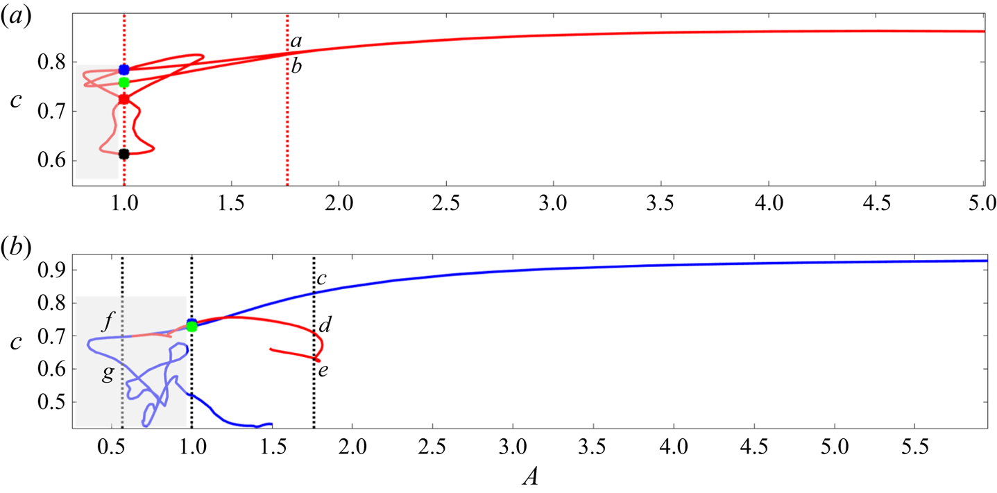
Figure 2 displays $c$-versus-$A$ continuation curves for rotationally symmetric ($k_0=2$) and rotationally asymmetric ($k_0=1$) TWs. The aspect ratio $A$ was used as a homotopy parameter while keeping $Re^{*}$ and $\alpha ^{*}$ constant. Red curves indicate solutions with shift-and-reflect symmetry, while blue curves represent TWs with an additional shift-and-rotate symmetry. Coloured markers on the curves indicate TWs for circular pipes when $A=1$ is used as the starting point of the continuation process. Again, it should be noted that $A>1$ corresponds to $\beta >0$, which means $Re_{ppf}=Re^{*}$ and $\alpha _{ppf}=\alpha ^{*}$ remain constant as $A$ varies. However, when $A<1$, within the grey rectangular regions, $Re_{ppf}$ and $\alpha _{ppf}$ will vary as $A$ changes. Even though these results are not physically comparable to $A>1$ solutions where $Re_{ppf}$ is preserved, for $A<1$ they are useful in generating new solutions, especially when $k_0=1$. In this case, the simple transformation ${\boldsymbol v(r,\theta ,z)}\rightarrow {\boldsymbol v(r,\theta +{\rm \pi} /2,z)}$ together with $A \rightarrow 1/A$ can be used to convert solutions for the aspect ratio $A<1$ to solutions for the aspect ratio $1/A>1$ for the same values of $Re^*$ and $\alpha ^*$, with $Re_{ppf}=A~Re^{*}$ and $\alpha _{ppf}=A~\alpha ^{*}$.

Figure 2.

The wave speed $c$ versus aspect ratio $A$ for TWs with (a) rotational symmetry when $(Re^{*}, \alpha ^{*})=(7500,1.55)$, and (b) rotational asymmetry when $(Re^{*}, \alpha ^{*})=(5000,1.437)$. Vertical dotted lines correspond to $A=1$, $A=1.76$ and $A=1/1.76$. Results for $A<1$ are shown in grey rectangular boxes. The velocity fields at the points labelled a–f are shown in figure 3.

In figure 2(a), results for rotationally symmetric ($\mathbb {R}_2$) TWs at $Re^{*}=7500$ and $\alpha ^{*}=1.55$ are shown. The blue, green, red and black markers at $A=1$ respectively denote the C2, C1, WK2 and WK branches of solutions of Ozcakir, Hall & Tanveer (Reference Ozcakir, Hall and Tanveer2019). The states C1 and C2 are centre modes, while WK and WK2 are VWI states. The WK2 and C2 branches possess shift-and-rotate $\varOmega _2$ symmetry in addition to the presumed shift-and-reflect $\mathbb {S}$ symmetry. Two continuation curves are generated, starting at a lower-branch WK solution, marked with a black dot, in the directions of increasing and decreasing aspect ratio $A$. Continuation curves cross the $A=1$ vertical line multiple times, creating a figure of eight in a narrow regime with small ellipticity $0.7< A<1.4$. The two branches merge at a bifurcation point $A\approx 1.94$, and only one TW branch exists for high aspect ratios. Figure 2(b) shows rotationally asymmetric ($\mathbb {R}_1$) TWs at $Re^{*}=5000$ and $\alpha ^{*}=1.437$. Coloured markers correspond to already known TW solutions of Pringle & Kerswell (Reference Pringle and Kerswell2007) for circular pipes: S1 (blue dot), M1 (green dot) and N1 (red dot). These TWs, except S1, possess the additional shift-and-rotate symmetry $\varOmega _1$, which is essentially a mirror symmetry about $\theta ={\rm \pi} /2$. In the regime of small ellipticity where $0.5< A<2$, multiple TWs exist, but as the ellipticity increases, only one branch survives, and it possess $\varOmega _1$ symmetry. This continuation curve is quite complex, becoming a somewhat tangled shape when $A<1$, because the two parameters ($Re_{ppf}$ and $\alpha _{ppf}$) vary as $A$ changes. One observation here is that the S1 solution is bifurcating from M1 at around $A\approx 0.7$ near the point labelled as (f), which shows that two distinct TWs in circular pipes are connected in the phase space when the geometry is perturbed slightly.

The perturbation velocity ${\boldsymbol v}$ can be written in the form ${\boldsymbol v} = {\boldsymbol U} (r, \theta ) + {\boldsymbol v}_w (r, \theta , z-ct )$ with zero axial average over a period, denoted by $\langle {\boldsymbol v}_w \rangle = 0$. 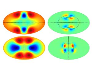If we write ${\boldsymbol U} (r, \theta ) = (U (r, \theta ), V(r, \theta ), W(r,\theta ) )$, then $(U (r, \theta ), V(r, \theta ), 0 )$ is referred to as the roll part of the flow and represents streamwise vortices; $(0, 0, W (r, \theta ) )$ is termed the streak, while ${\boldsymbol v}_w (r, \theta , z-ct)$ represents the wave part of the flow. Figure 3 displays the cross-sectional velocity profiles for the streaks (left) and the waves (right) at the corresponding labelled points in figure 2. As described in the introduction, the structure and mechanism of TWs have been addressed by Hall & Sherwin (Reference Hall and Sherwin2010). Therefore, it is of interest to illustrate TWs found here in relation to the critical layer position. The black curves in the right-column contour plots show the position of the critical curve defined by $1-r^2 +W(r,\theta )=c$. The axis of mirror symmetry is shown by a dashed line in figure 3(e–g). In all plots, the streaks remain the same size throughout the pipe, until wall effects become important. Figure 3(a,b) displays velocity fields corresponding to points labelled a and b in figure 2(a), with $k_0=2$, where the wave component of TWs are localized inside a core region and exhibit relatively strong deviations near the centre of the pipe. Figure 3(c–g) shows velocity fields that correspond to points labelled c–g in figure 2(b), for $k_0=1$, where the wave intensity is largest in a layer around the critical curve, as shown. Figure 3(f,g) with $A=1/1.76$ is particularly interesting, because these solutions give rise to TWs which possess top–bottom symmetry without its having been imposed numerically in the solver.

Figure 3.

The cross-sectional velocity profiles for streaks (left) and waves (right) at corresponding points on figure 2 when $\tilde {z}=0$ for $A=1.76$ (a–e) and $A=1/1.76$ (f,g). Contour colours range from dark red (largest positive) to dark blue (smallest negative). The black dashed lines in (e–g) show the axes of mirror symmetry. In (f,g), $Re_{ppf}=2840.9$, and the results are displayed after a ${\rm \pi} /2$-radian clockwise rotation around the origin.

For large values of the aspect ratio $A$, new TW solutions are obtained by a continuation of the points labelled a and c in figure 2. The cross-sectional velocity profiles are shown in figures 4 and 5, respectively. In both figures 4(a) and 5(a), the streaks are becoming more localized around the pipe centre along the major axis; the critical layers stay close to the centre as $A$ increases. In figure 4(b) the waves remain concentrated in a core region and appear to expand between just above the critical layer and the pipe centre, while in figure 5(b) the waves are largest around the critical layer. The clear organization of waves around the critical layer suggests suggests a connection to the critical layer dynamics of VWI.

Figure 4.

The cross-sectional plots of the perturbation velocity at $\tilde {z}=0$ for streaks (a) and waves (b) for aspect ratio $A=6.51$ when $(Re^{*},\alpha ^{*})=(7500,1.55)$ with $k_0=2$.

Figure 5.

The cross-sectional plots of the perturbation velocity at $\tilde {z}=0$ for streaks (a) and waves (b) for aspect ratio $A=9.38$ when $(Re^{*},\alpha ^{*})=(5000,1.437)$ with $k_0=1$.

Other classes of TWs can be obtained at high aspect ratios after careful investigation of the solutions in figure 2(b) by continuously increasing $Re^{*}$ and decreasing the aspect ratio $A$. For example, starting at the point f, whose cross-section is shown in figure 3(f), we are able to compute a new TW at $A=1/5.56$ to the desired accuracy as shown in figure 6. After a rotation by ${\rm \pi} /2$ radians, this TW has top–bottom mirror symmetry with $A=5.56$, and it has a wide, almost elliptical critical layer, with localized waves concentrated around the critical curve. Similar calculations can be done at the other labelled point g, but because of the computational cost, we did not attempt to do such calculations with high accuracy.

Figure 6.

Cross-sectional plots of the perturbation velocity at $\tilde {z}=0$ for streaks (a) and waves (b). (c) Contour lines of the magnitude of the fundamental Fourier harmonics $\| {\boldsymbol u}_1(r,\theta )\|$, where ${\boldsymbol u}(r,\theta , z)=\sum _{l=-P}^P {\boldsymbol u}_l(r,\theta ) e^{ i\alpha l z}$ when $A=1/5.56$ and $(Re^{*},\alpha ^{*})=(5000, 0.2719)$ with $k_0=1$ and $Re_{ppf}=899.28$. Plots are rotated ${\rm \pi} /2$ radians clockwise, and only the upper half of the pipe is shown, because of top–bottom mirror symmetry.

Figure 7 displays the wave speed $c$ of TWs as a function of $Re_{ppf}$ for $k_0=1$ (black) and $k_0=2$ (blue) solution branches for the aspect ratios $A=1.76$ (solid), $A=1/1.76$ (dash-dotted), $A=3.36$ (dashed) and $A=9.38$ (dotted). The rotationally symmetric solutions ($k_0=2$) arise at much larger values of $Re$ than the asymmetric solutions ($k_0=1$). The points labelled a–g in figure 2 are also marked as reference points, with the corresponding flow fields shown in figure 3. All of the TWs (except for $A=9.38$) arise from saddle-node bifurcations. For each $c$-versus-$Re_{ppf}$ curve, the two branches emanating from the saddle-node bifurcation point are identified as the ‘upper’ and ‘lower’ branches depending on whether they have lower or higher drag, similarly to their counterparts for circular pipes. Results suggest that TWs without any discrete rotational symmetry exist at much lower Reynolds numbers. From left to right, the first TW solution, which is a rotationally asymmetric TW with $A=1/1.76$, appears to first exist at the saddle node point $Re_{ppf}=933$. This solution has top–bottom mirror symmetry after a ${\rm \pi} /2$-radian rotation around the origin. Next, another rotationally asymmetric solution with left–right mirror symmetry is born out of a saddle node bifurcation at $Re_{ppf}=968$ with $A=1.76$. As $Re_{ppf}$ increases, other asymmetric solution branches appear at different aspect ratios. Because of the computational costs, only the lower branch is computed for $A=9.382$; therefore, the saddle-node point for that branch is not known. For rotationally symmetric solutions, there are two solution branches for $A=1.76$, with saddle-node points at $Re_{ppf}=3638$ and $Re_{ppf}=6817$, and one solution branch for $A=3.36$, originating at $Re_{ppf}=5981$.

Figure 7.

The $Re_{ppf}$ versus $c$ for elliptical pipes at various aspect ratios $A$ for $k_0=1$ (black) and $k_0=2$ (blue): $A=1.76$ (solid), $A=1/1.76$ (dash-dotted), $A=3.36$ (dashed) and $A=9.38$ (dotted). When $k_0=2$, $\alpha _{ppf}=1.55$; when $k_0=1$, $\alpha _{ppf}=1.437$ for $A>1$ and $\alpha _{ppf}=0.816$ for $A<1$. The labels a–g correspond to the points a–g in figure 2.