1. INTRODUCTION
Let {yt} be a stationary autoregressive moving average (ARMA) time series generated by the equation

where the innovation process {εt} is a sequence of independent and identically distributed (i.i.d.) random variables and β = (φ1,…, φp,θ1,…, θq)′ is an unknown parameter vector. When Eεt2 < ∞, it is well known that various estimators such as the maximum likelihood estimator (MLE), Whittle estimators, and least squares estimators (LSE) for β are all asymptotically normal and unbiased (Brockwell and Davis, 1991). Furthermore, the least absolute deviations estimator (LADE) is also asymptotically normal; see Dunsmuir and Spencer (1991) and Davis and Dunsmuir (1997). When Eεt2 = ∞, model (1.1) is called the infinite variance ARMA (IVARMA) model, which defines a heavy-tailed process {yt}. The IVARMA models are pertinent in modeling heavy-tailed time series data often encountered in, for example, economics and finance (Koedijk, Schafgans, and De Vries, 1990; Jansen and de Vries, 1991). For further references on statistical modeling for heavy-tailed phenomena, we refer to Resnick (1997) and Adler, Feldaman, and Taqqu (1997).
Statistical inference for IVARMA models has not been well explored yet. Most available results concern infinite variance autoregressive (IVAR) models (i.e., q = 0 in (1.1)). Gross and Steiger (1979) and An and Chen (1982) obtained the strong consistency and the convergence rates for LADE for IVAR models. Davis and Resnick (1985, 1986) derived the limiting distributions of the LSE for IVAR models. A more comprehensive asymptotic theory of M-estimators for autoregressive (AR) models was derived by Davis, Knight, and Liu (1992). For IVARMA models, the asymptotic properties for several estimators have been derived when the innovation distribution is in the domain of attraction of a stable law distribution with index between 0 and 2. For example, both the Whittle estimator proposed by Mikosch, Gadrich, and Adler (1995) and the Gauss–Newton estimator proposed by Davis (1996) converge in distribution to some functions of a sequence of stable random variables. Furthermore, it has been proved that the M-estimator converges in distribution to the minimizer of a stochastic process; see Davis (1996) and Calder and Davis (1998). Kokoszka and Taqqu (1996) extended the results of Mikosch et al. (1995) to fractional ARMA models with infinite variance. However, all the preceding limiting distributions are complicated and depend intimately on the unknown tail indices of the underlying processes. This makes it difficult to develop asymptotic approximations for the purpose of statistical inference. This paper provides a remedy for this problem.
The difficulty of the asymptotic theory for LADE for IVARMA processes may at least partially result from the fact that the residual of a linear prediction for yt based on its lagged values depends on β nonlinearly, whereas such a dependence is completely linear for pure AR processes. Note that this linearity implies that the objective function for least absolute deviations estimation is convex and therefore the asymptotic normality of LADE may be readily derived from the convex lemma (Hjort and Pollard, 1993). One way to deal with a nonconvex objective function is to adopt a local linearization around the true value of the parameter, which enables one to establish asymptotic properties of a local estimator defined as a local minimizer around the true value of the parameter. This is the line taken in the paper by Davis and Dunsmuir (1997), which dealt with LADE for ARMA models with Eεt2 < ∞. On the other hand, Ling (2005) proposed a weighted least absolute deviations estimator (WLADE) for IVAR models. The key idea of the WLADE is to weigh down the observations that are excessively large, either positively or negatively. Ling (2005) showed that the WLADE is asymptotically normal. The idea of weighing down the large observations has also been used in estimation for autoregressive conditionally heteroskedastic (ARCH) models with heavy tailed innovations by Horvath and Liese (2004).
In this paper, we deal with the WLADE for IVARMA models. By adopting the idea of local linearization mentioned previously, we show that a local WLADE is asymptotic normal and unbiased under the condition that E|εt|δ < +∞ for some δ > 0 and the density function of εt and its derivative are bounded. This facilitates statistical inference for IVARMA models (even when E|εt| = ∞) in a conventional fashion. For example, a Wald test for a linear hypothesis can be constructed; see Section 2. For relatively small samples a simulation study indicates that the proposed WLADE is more accurate than the Whittle estimator, the quasi-maximum-likelihood estimator (QMLE), and the Gauss–Newton estimator when Var(εt) = ∞. Furthermore, the efficiency loss of the WLADE with respect to the (unweighted) LADE is not significant with appropriately selected weights. Because the WLADE converges at a slower rate than the Whittle estimator and the Gauss–Newton estimator, we also studied the large-sample properties of the WLADE numerically.
Although we only deal with IVARMA models in this paper, the basic idea of combining a weighted objective function with local linearization of the residuals may apply to other infinite variance time series models, such as the infinite variance autoregressive integrated moving average (ARIMA) and the integrated generalized autoregressive conditionally heteroskedastic (IGARCH), which are popular in financial econometrics. Another open problem is to develop appropriate methods for choosing weight functions; see Remark 3 in Section 2.2.
The rest of paper is organized as follows. The WLADE and the associated asymptotic properties are presented in Section 2. In addition to showing the asymptotic normality of the local WLADE, we also show that a (global) estimator sharing the same asymptotic property could be obtained by minimizing a convex objective function if there is available an initial estimator within root-n distance from the true value; see Theorem 2 in Section 2.2. Section 3 gives all the theoretical proofs of the results in Section 2. Section 4 reports some numerical results from a simulation study.
2. WLADE AND ITS ASYMPTOTIC PROPERTIES
2.1. Weighted Least Absolute Deviations Estimators
Denote by Θ ⊂ Rp+q the parameter space that contains the true value β0 = (φ10,…, φp0,θ10,…, θq0)′ of the parameter β as an inner point. For β = (φ1,…, φp,θ1,…, θq)′, put

where yt ≡ 0 for all t ≤ 0. Note that εt ≠ εt(β0) because of this truncation.
We define the objective function as

and the WLADE as

where u = u(n) is a positive integer and the weight function, depending on a constant α > 2, is defined as

2.2. Asymptotic Normality of WLADE
To state the asymptotic normality of

, we introduce some notation first. Let

It is easy to see that

, where

is a minimizer of

Denote At(β) = (At,1(β),…, At,p+q(β))′, where At,i(β) = −∂εt(β)/∂βi. By (8.11.9) of Brockwell and Davis (1991), it holds for t ≥ max(p,q) that

where B is the backshift operator.
For t = 0,±1,±2,…, define

Put Qt = (Ut−1,…,Ut−p,Vt−1,…,Vt−q)′,

, and

We denote by ∥v∥ the euclidean norm for a vector v.
Some regularity conditions are now in order.
A1. For β ∈ Θ, the polynomials θ(z) = 1 + θ1 z + ··· + θq zq and φ(z) = 1 − φ1 z − ··· − φp zp have no common zeros, and all roots of φ(z) and θ(z) are outside the unit circle.
A2. Innovation εt has zero median and a differentiable density function f (x) satisfying the conditions f (0) > 0, supx∈R| f (x)| < B1 < ∞, and supx∈R| f′(x)| < B2 < ∞. Furthermore, E|εt|δ < +∞ for some δ > 0, and α > max{2,2/δ}.
A3. As n → ∞, u → ∞ and u/n → 0.
The following proposition indicates that model (1.1) has a unique strictly stationary and ergodic solution under conditions A1 and A2.
Proposition 1. Suppose that condition A1 holds and E|εt|δ < +∞ for some δ > 0. Then model (1.1) defines a unique strictly stationary and ergodic process {yt}.
Proof. Condition A1 implies that

where |ψj| ≤ Crj for some constants C > 0 and 0 < r < 1. Let

. Then

The same argument as for Proposition 13.3.2 of Brockwell and Davis (1991) yields the result. █
Remark 1. Condition A3 eliminates asymptotically the bias in the estimation resulting from the lack of observations yt for t ≤ 0.
Remark 2. Condition A2 does not rule out the possibility that E|εt| = ∞. The purpose of introducing weights

is to weigh down excessively large observations that reflect the heavy-tailed innovation distribution. Therefore the asymptotic covariance matrix of the normalized WLADE, depending on Σ and Ω given in (2.7), is a well-defined (finite) matrix. Note that

. Conditions A1 and A2 imply that for

,

Hence

with probability one, which ensures that wt is well defined. Note that wt is stationary and ergodic under condition A1 and it is asymptotically equivalent to

for t > u (see A3).
We are now ready to state our main results.
THEOREM 1. Let conditions A1–A3 hold. For any given positive random variable M with P(0 < M < ∞) = 1, there exists a local minimizer

of Wn(β) that lies in the random region

for which

where ξ is a normal random vector with mean 0 and covariance matrix (1/4f2(0))Σ−1ΩΣ−1.
Notice that the lack of convexity for the objective function Wn(β) complicates the search for its minimizer. As in Davis and Dunsmuir (1997), Wn(β) may be linearized in a neighborhood of a good initial estimate

as follows:

The resulting estimator

shares the same asymptotic property as the local WLADE. See Theorem 2, which follows.
THEOREM 2. Let conditions A1–A3 hold. Then

provided that

.
Remark 3. Although we only deal with the weight function defined in (2.4) explicitly, the preceding theorem holds for general weight function gt ≡ g(yt−1,yt−2,…) provided

where

,

, 0 < r < 1, and C0 > 0 are constants. For example, we may use weights of more general form:

The numerical examples in Section 3 indicate that the accuracy of the WLADE is not sensitive with respect to the value of α. However the choice of γ = 2 typically leads to a better estimator than those with γ > 2, at least for model (4.1). Furthermore, it seems that d = 2,3,4 behave almost equally well. However how to choose a weight function in general such that the resulting estimator is of certain optimality remains an open question.
2.3. A Wald Test for Linear Hypotheses
The asymptotic normality of the estimator

stated in Theorem 1 facilitates inference for model (1.1). For example, we may consider a general form of linear null hypothesis:

where Γ is an s × (p + q) constant matrix with rank s and κ is an s × 1 constant vector. A Wald test statistic may be defined as

and we reject H0 for large values of Zn. In the preceding expression,

Here

is defined in the same manner as Qt but with β0 replaced by

, εt replaced by

, and yt = 0 for all t ≤ 0 (see (2.6) and (2.7)), and

is an estimate for f (0) defined as

where K(·) is a kernel function on R and bn > 0 is a bandwidth. Theorem 3, which follows, shows that the asymptotic null distribution of Zn is χs2. It in fact still holds if

in the definition of Zn is replaced by

.
THEOREM 3. Suppose conditions A1–A3 hold. Let kernel function K be bounded, Lipschitz continuous, and of finite first moment. Let bn → 0 and nbn4 → ∞ as n → ∞. Then

under H0.
3. PROOFS
We use the same notation as in Section 2. For any fixed v ∈ Rp+q, put

We linearize εt(β) around β0; that is, εt(β) is approximated by

where At(β) is defined in (2.5).
We denote by

the convergence in distribution and by

the convergence in probability. Let C(Rs) be the space of the real-valued continuous functions on Rs (Rudin, 1991). For probability measures Pn and P on C(Rs), we say that Pn converges weakly to P in C(Rs) if ∫fdPn → ∫fdP for any bounded and continuous function f defined on C(Rs). For random functions Sn,S defined on C(Rs),

if the distribution of Sn converges weakly to that of S in C(Rs) (Billingsley, 1999). The term C denotes a positive constant that may be different at different places.
3.1. Proof of Theorem 1
Before we prove Theorem 1, we first introduce a proposition that is of independent interest. Its proof is divided into several lemmas. We always assume that conditions A1–A3 hold.
PROPOSITION 2. As n → ∞, it holds that

on C(Rp+q), where T(v) = f (0)v′Σv + v′N and N denotes an N(0,Ω) random vector.
LEMMA 1. It holds that |εt − εt(β0)| ≤ ξt and |At,i(β0) − Qt,i| ≤ ξt for i = 1,…, p + q, where

, 0 < r < 1, C0 is a positive constant, and Qt,i is the ith component of Qt.
Proof. See Brockwell and Davis (1991, pp. 265–268).
LEMMA 2.

on C(Rp+q).
Proof. We first prove the convergence for any fixed v. Using the identity

which holds for z ≠ 0, we have

Notice that, by Lemma 1, we have

and

Then, Ewt2(Qt′v)2 < +∞. But, from conditions A1 and A2, {wtQt′vsgn(εt)} is a stationary martingale difference sequence. Therefore, applying a martingale central limit theorem (Hall and Heyde, 1980), we obtain

.
For Bn, let

and

. Then

Similarly to (3.1), we can obtain

Therefore, we have proved that

On the other hand, on the set {Qt′v > 0}, we may show that

and

see Davis and Dunsmuir (1997). Therefore,

Using the same argument for the second indicator in the summands of Bn, we obtain that

so that the finite-dimensional distributions of Sn+ converge to those of T. But because Sn+ has convex sample paths, this implies that the convergence is in fact on C(Rp+q) (see Davis and Dunsmuir, 1997, proof of Prop. 1). █
LEMMA 3.

uniformly on compact sets.
Proof. Notice that

First, we consider

By Lemma 1 and the proof of (3.1), we know that

Then

uniformly on compact sets. For K1, we have

uniformly on compact sets, because we have the facts

Therefore,

uniformly on compact sets as n → ∞.
Now we consider

By a method similar to the proof for K2, we can obtain that

uniformly on compact sets. On the other hand, denote ηt = εt(β0) − εt. It can be verified that

Then from condition A3 and by a method similar to the proof of Lemma 2, we have

By the same method as for K1, we can obtain that D21 → 0. On the other hand,

Therefore, we have

And we can obtain E|D3| → 0 similarly to (3.5). Hence

uniformly on compact sets.
By the same method as for Λ2, we have

uniformly on compact sets. This completes the proof of this lemma. █
LEMMA 4.

uniformly on compact sets.
Proof. Notice that we have the fact that under conditions A1 and A2, for any given positive number M, there exist positive constants C > 0 and 0 < r < 1 such that for sufficiently large n

Now we have

as n → ∞, by conditions A2 and A3 and the fact that (h + t)−α ≤ 2−α(ht)−α/2. This completes the proof of Lemma 4. █
Proof of Proposition 2. For v ∈ Rp+q, define

where

From the definition of εt(β) in expression (2.1), we have

Similarly, replacing At−i,j (or At−j,i) by Qt−i,j (or Qt−j,i) in the preceding three equalities, we can define Xt = (Xt(i,j)). Then, (ht(i,j)(β0)) can be well approximated by (Xt(i,j)) such that

which can be proved in the same way as Lemma 1.
Notice that

Notice that

; we obtain

by (3.6). Using the same argument of E|K1| → 0 in Lemma 3, we have

. Similarly, we have

Let

and

In the same way as the proofs of (3.3) and (3.5) for T21(1) and T21(2), respectively, we can obtain that

. The same result holds for the rest term of T2. Thus, it follows that

uniformly on compact sets.
But,

where βn* is between β0 and β0 + n−1/2v. Then,

uniformly on compact sets. Therefore, combining Lemmas 3 and 4, we have

uniformly on compact sets.
By Lemma 2, we obtain that

as n → ∞. This completes the proof. █
Proof of Theorem 1. Note that the limit process in Proposition 2 has convex sample paths and a unique minimizer:

Let Pn and P be the probability measures on C(Rp+q) induced by Tn and T, respectively. By Skorokhod's representation theorem (cf. Pollard, 1984, pp. 71–73), there exists a probability space

with processes T* and Tn* having the distributions P and Pn, respectively, such that

. Hence, there exists a subset Ω′ of Ω* with P*(Ω′) = 1 such that for any ω ∈ Ω′,

holds for any compact set K. Denote the minimizer of T* by ξ*. Then ξ* has the same distribution as ξ. For any given positive random variable M, let

Now we show that ξn*(ω) → ξ*(ω). Suppose ξn*(ω) → ξ*(ω) does not hold; then there is a subsequence n′ such that ξn′*(ω) → ξ′(ω) ≠ ξ*(ω) and we know ∥ξ′(ω) − ξ*(ω)∥ ≤ M(ω). From the definition of ξn*(ω), we have

But, on the other hand,

From (3.7), we can obtain that G1 → 0 and G3 → 0. Noticing that T*(v,ω) is continuous, we have

This is a contradiction. Therefore,

.
Define a sequence of local minimizers {ξn} of Tn by

Then, ξn converges in distribution to ξ. The proof is completed. █
3.2. Proof of Theorem 2
We also use the substitution

. Then, minimizing

is equivalent to minimizing

Because

has convex sample paths, we only need to prove that

on C(Rp+q) by Lemma 2.2 in Davis et al. (1992).
Denote

By Taylor expansion near

, for any fixed v ∈ Rp+q, we have

where β1t lies between

and β0 + n−1/2v. We now have

where β2t lies between β0 and β0 + n−1/2v. Hence, by a similar way to the proof of Lemma 2 but replacing n−1/2Qt′v by

, we have

█
3.3. Proof of Theorem 3
Based on Theorem 1, Theorem 3 follows immediately from Lemmas 5 and 6 in this section. We assume that the conditions of Theorem 3 hold.
LEMMA 5.

and

.
Proof. Denote

Then

where

and

are determined by

Note that, by the definition of εt(β), we have

where yt = 0 for t ≤ 0. Hence,

Let

Then,

. Obviously, II2 → Σ by the ergodic theorem. For II1, we first define a vector-valued function Qt(β) = (Ut−1(β),…,Ut−p(β),Vt−1(β),…,Vt−q(β))′, and its components are determined as follows:

We denote

and divide II1 into three terms as follows:

It is easy to obtain that

by Lemma 1 and the definition of

. Notice that the (1,1)th element of J2 is

and

for some positive constant C and ξt defined in Lemma 1. It follows that

, and similarly we can prove that the rest elements of J2 converge to zero in probability. Hence

. For J3, noticing that Qt = Qt(β0), we have

where βt* lies between

and β0. Noticing that wt1/2∥(∂Qt(β*))/∂β′∥ ≤ C, wt1/2∥Qt∥ ≤ C, and

, we obtain that

. Now it has been proved that

.
In the same way we can prove

. █
LEMMA 6. It holds that

.
Proof. Define

where

; then

where

. So we need to prove that

Notice that

where

But, Lipschitz continuity of K(x) insures that there exists a positive number L such that |K(x) − K(y)| ≤ L|x − y| for any x,y, and then, from Theorem 1 and the assumptions on bn, we have

where β* lies between

and β0. For P2, equivalently we need to prove that

In fact,

where

Notice that

But

by the assumptions on K(x), and

by condition A3 and the assumptions on K(x). Noticing that

, we have (3.8). The proof of Lemma 6 is completed. █
4. NUMERICAL PROPERTIES
We conducted a simulation study to illustrate the finite-sample properties of the proposed WLADE in five aspects: namely, (i) its accuracy; (ii) its sampling distribution; (iii) comparison with the unweighted LADE, the Whittle estimator (Mikosch et al., 1995), QMLE, and the Gauss–Newton estimator (Davis, 1996); (iv) the selection of α, γ, and d in (2.8); and (v) the performance of the Wald test statistic Zn.
We generated data from a simple ARMA(1,1) model:

with t2, Cauchy, or N(0,1) innovation distribution. Unless specified otherwise, we always set u = 20, α = 3, and d = 0.
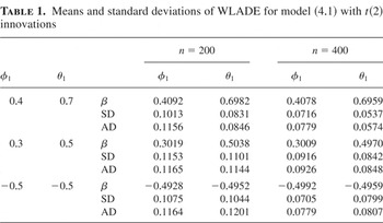
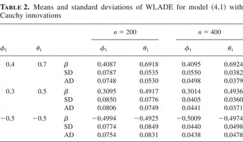
Tables 1 and 2 list the means and the standard deviations (SD) of the WLADE for φ1 and θ1 from the 1,000 samples from model (4.1) with sample size n = 200 or 400 and the true value (φ1,θ1) = (0.4,0.7), (0.3,0.5), or (−0.5,−0.5). The estimates are very accurate in general, and the accuracy increases when the sample size increases from 200 to 400. We also included in the tables asymptotic standard deviations (AD) derived from Theorem 1 with (Σ,Ω) replaced by their estimators in (2.9) and with f (0) replaced by (2.10) with the kernel K(x) = e−x/(1 + e−x)2 and the rule-of-thumb bandwidth bn = 1.06 × n−1/5 (Silverman 1986, p. 40). The values of SD and AD are quite close to one another.
Means and standard deviations of WLADE for model (4.1) with t(2) innovations

Means and standard deviations of WLADE for model (4.1) with Cauchy innovations

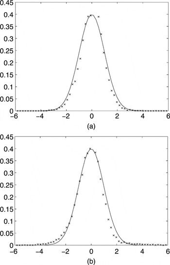
To investigate the sampling distributions of the WLADE, we drew 16,000 samples of size n = 400 from (4.1) with (φ1,θ1) = (0.3,0.5) and t2 or Cauchy innovations. For each sample, the WLADEs for both φ1 and θ1 were obtained. We divided [−6,6] into small intervals with equal length 0.2. For each small interval, we computed the (normalized) relative frequency for the occurrence of the event that the normalized WLADE falls into the interval. Those relative frequencies are plotted against the center of intervals in Figures 1 and 2. We superimposed the N(0,1) density function in the figures, which is the limiting density of the normalized WLADE. Even with sample size n = 400, the estimated values of the density functions match their asymptotic limits very well.

Estimated values (×) for the density functions of the normalized (shown in (a)) and (shown in (b)), together with their asymptotic limit—the N(0,1) density (solid curves) for model (4.1) with t2 innovations.

Estimated values (×) for the density functions of the normalized (shown in (a)) and (shown in (b)), together with their asymptotic limit—the N(0,1) density (solid curves) for model (4.1) with Cauchy innovations.
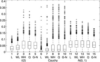
Figure 3 presents the box plots of the average absolute error (AAE)

for the unweighted LADE, the WLADE, the Whittle estimator, the QMLE, and the Gauss–Newton estimator from 1,000 samples with sample size n = 400 drawn from (4.1). Here, we set d = 2. For the samples with heavy-tailed innovations, that is, t2 and Cauchy, the WLADE performed better than the Whittle estimator, QMLE, and the Gauss–Newton estimator. In fact, the improvement from using the WLADE over the preceding three estimators is more pronounced when the tails are heavier (i.e., with Cauchy distribution). The Gauss–Newton estimator performed the best with Gaussian innovations. However it is noticeable that there was an efficiency loss due to the introduction of weights in the estimation, although such a loss was not significant at least in the setting used in our simulation.

Box plots of the AAE of LADE (L), WLADE (WL), Whittle estimator (WH), QMLE (Q) and Gauss–Newton estimator (G–N) for model (4.1).
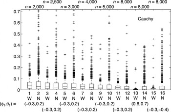
Because the convergence rate of the WLADE is slower than the Gauss–Newton estimator (Mikosch et al., 1995; Davis, 1996), we compared the two estimators with large sample size n between 2,000 and 8,000. For each setting, 1,000 samples were drawn from model (4.1) with Cauchy innovations. The parameters (φ1,θ1) were set at (−0.3,0.2), (0.3,−0.5), (−0.3,0.5), (0.1,−0.6), (0.3,0.5), (0.6,0.7), (0.4,0.6), (−0.4,−0.6), (−0.3,−0.4), and

. It turned out that when φ1θ1 > 0, the WLADE performed better than the Gauss–Newton estimator for all n ≤ 8,000. However, when φ1θ1 < 0, the WLADE was better than the Gauss–Newton estimator only for n ≤ 3,000. The box plots of the AAE for parameters (φ1,θ1) = (−0.3,0.2),(−0.3,−0.4),(0.6,0.7) are displayed in Figure 4.

Box plots of the AAE of WLADE (W) and Gauss–Newton (N) estimator for model (4.1) for the large-sample case.
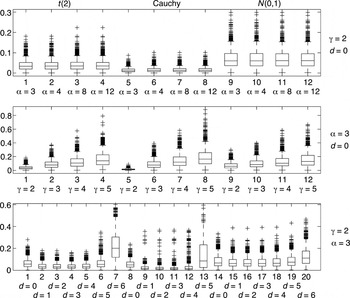
We also compared the WLADE using a general form of weights (2.8) with different α, γ, and d. To this end, we drew 1,000 samples from model (4.1) with (φ1,θ1) = (0.3,0.5) and n = 400. Figure 5 presents the box plots of the AAEs with t2, Cauchy, and normal innovations. They suggest that the WLADE is fairly robust with respect to the value of α. However, the WLADE is more sensitive to γ. It is evident that we should choose γ as small as possible, that is, γ = 2, which corresponds to the default weight function used in this paper. On the other hand, the performances with d = 1,2, and 3 do not differ significantly.

Box plots of AAE of WLADE with different α, γ, and d for model (4.1).
Finally, we approximated the P-value of the Wald test proposed in Section 2.3 for testing AR(1) against ARMA(1,1) models by the relative frequency

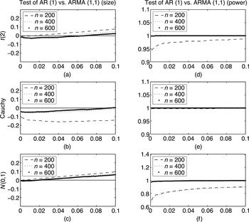
for the occurrence of the event that the AR(1) null hypothesis was rejected in a simulation with 1,000 replications. The data were generated from (4.1) with (φ1,θ1) = (0.3,0) or (φ1,θ1) = (0.3,0.5) and innovation to be t(2), Cauchy, or N(0,1). We repeated the experiment with sample size equal to, respectively, 200, 400, and 600 for the nominal significance level between 0 and 0.1. Figure 6 plots the difference between

and the nominal significance level against the nominal level with data generated from (4.1). With (φ1,θ1) = (0.3,0), Figure 6(a)–(c) indicate that the χ2-asymptotic approximation for the significance level is accurate, especially for n = 400 and 600. With (φ1,θ1) = (0.3,0.5), Figure 6(d)–(f) illustrate that the test is powerful in detecting the departure from the AR(1) hypothesis.

Simulation results for the Wald test. Differences between approximated P-value and the nominal significance level are plotted against the nominal level. The data were generated from (4.1) with (φ1,θ1) = (0.3,0) for (a)–(c) and (φ1,θ1) = (0.3,0.5) for (d)–(f).