1 Introduction
In accident scenarios such as industrial explosions from the leakage of combustible gas (Auban, Zboray & Paladino Reference Auban, Zboray and Paladino2007), detonation often propagates in a non-homogeneous medium which, however, is frequently not taken into account in the prediction of explosion hazards. Another relevant application is rotating detonation engines for which detonation stability may depend on the degree of non-uniformity. Consequently understanding detonation propagation in mixtures with concentration gradients is of both fundamental interest and practical relevance. Studies have been conducted of concentration gradients that are either parallel or perpendicular to the propagation direction. Regarding the former, Thomas, Sutton & Edwards (Reference Thomas, Sutton and Edwards1991) generated a concentration gradient by allowing unburned gas, initially separated by a slide, to diffuse for a given time. They produced gradients by varying the length of time between the removal of a horizontal sliding plate that separated two different gas mixtures and the initiation of the detonation. It was found that for a steeper gradient, detonation is less likely to survive because it has less time to adapt to the new environment. Kuznetsov et al. (Reference Kuznetsov, Dorofeev, Efimenko, Alekseev and Breitung1997, Reference Kuznetsov, Alekseev, Dorofeev, Matsukov and Boccio1998) studied experimentally the propagation, decay and re-initiation of detonation through a concentration gradient of variable width into a less reactive acceptor mixture, and found that propagation and quenching depended significantly on the sharpness of the concentration gradient. Furthermore, Sochet, Lamy & Brossard (Reference Sochet, Lamy and Brossard2000) examined experimentally the detonability of a non-uniform mixture, which was created by diffusion of a gaseous mixture initially confined in a hemispherical volume into the surrounding air when the confinement was ruptured. Based on the pressure profiles of the blast waves generated by the explosion, the limit between the two explosion phenomena, namely total and partial explosive charge, is defined. Oran, Jones & Sichel (Reference Oran, Jones and Sichel1992) found several shock structures along the interface of an initially segregated and diluted hydrogen–oxygen mixture, the details of which depend on the relative reactivity of the upper and lower mixtures and the overdriven degree of detonation in the primary mixture. Recently, Mi, Timofeev & Higgins (Reference Mi, Timofeev and Higgins2017) studied numerically gaseous detonation propagation in a spatially inhomogeneous medium and found interestingly that detonation velocity is higher than the Chapman–Jouguet (CJ) speed and the deviation above the CJ velocity increases as the sources are made increasingly discrete. They explained that for highly discrete sources the deviation above the CJ velocity is due to the effective sonic surface not corresponding to an equilibrium state through averaging detonation structure.
Regarding propagation through a normal concentration gradient, Lieberman, Shepherd & Brossard (Reference Lieberman, Shepherd and Brossard2007) created a concentration gradient by the formation of a gravity current using a sliding valve that initially separated test gas and combustible mixture. Detonation in the concentration gradient has a curved front, and the leading shock and reaction front decouple due to the sharp rise in the induction time in regions where the diluent is the dominant species. Ishii & Kojima (Reference Ishii and Kojima2007) experimentally found that the inclination of the detonation front increased with a steepening concentration gradient, and the propagation speed was less than the ideal CJ velocity in a stoichiometric mixture. After a specified diffusion time, a detonation was initiated in the test section. Schlieren images showed that the detonation front is curved in the region where the fuel was most diluted, with smaller curvature for smaller effective concentration gradients. Detonation cells were also recorded by using smoke foil, showing that inside the concentration gradient, the detonation cells resemble parallelograms and are larger than those formed near the opposite wall of the test section where the mixture is nearly stoichiometric. Vollmer, Ettner & Sattelmayer (Reference Vollmer, Ettner and Sattelmayer2012) and Wang & Wen (Reference Wang and Wen2017) studied experimentally and numerically the entire deflagration to detonation transition in mixtures with a transversal concentration gradient. Boeck et al. (Reference Boeck, Berger, Hasslberger and Sattelmayer2016) experimentally observed single-head propagation with strong transverse wave and multi-head propagation with a constant macroscopic front curvature. Calhoon & Sinha (Reference Calhoon and Sinha2005) numerically identified the triple-shock structure of two-dimensional detonation by setting an inflow boundary with a hyperbolic tangent function, but without considering transverse instabilities. Oran et al. (Reference Oran, Jones and Sichel1992, Reference Oran, Weber, Stefaniw, Lefebvre and Anderson1998) and Kessler, Gamezo & Oran (Reference Kessler, Gamezo and Oran2011, Reference Kessler, Gamezo and Oran2012) simulated detonation propagation and quenching in spatially varying fuel concentrations with a calibrated one-step reaction, by which one-dimensional detonation properties of model mixtures are similar to those observed in a typical hydrocarbon–air mixture. They observed an unreacted pocket appearing behind the front of the detonation in the non-homogeneous mixture. Ettner, Vollmer & Sattelmayer (Reference Ettner, Vollmer and Sattelmayer2010, Reference Ettner, Vollmer and Sattelmayer2013) considered the role of realistic reactions (Oran et al.
Reference Oran, Jones and Sichel1992) and used detailed
 $\text{H}_{2}{-}\text{O}_{2}$
reactions to describe inclined detonation front and distorted cell, showing an increase in cell size and irregularity with concentration gradient change.
In uniform mixtures, several previous works showed evidence of unreacted fuel passing through the reaction zone (Oran et al. Reference Oran, Young, Boris, Picone and Edwards1982; Austin Reference Austin2003; Pintgen et al. Reference Pintgen, Eckett, Austin and Shepherd2003; Radulescu Reference Radulescu2003; Austin, Pintgen & Shepherd Reference Austin, Pintgen and Shepherd2005; Radulescu et al. Reference Radulescu, Sharpe, Lee, Kiyanda, Higgins and Hanson2005; Sabzpooshani & Mazaheri Reference Sabzpooshani and Mazaheri2009; Mahmoudi & Mazaheri Reference Mahmoudi and Mazaheri2010; Mahmoudi et al. Reference Mahmoudi, Karimi, Deiterding and Emami2014) when the fresh gas becomes detached from the front. An unreacted pocket behind the detonation front has been observed for highly irregular detonations (Subbotin Reference Subbotin1975). Gamezo, Desbordes & Oran (Reference Gamezo, Desbordes and Oran1999) found numerically that consumption of the unreacted pockets appearing behind the front is related to detonation instabilities associating with mixture properties. For highly unstable detonations, unreacted pockets are observed downstream of the front, while they are not formed for stable detonations. However, if the average detonation velocity is sufficiently low, as for example for a marginal wave in a narrow channel, then unreacted pockets are possible in all mixtures. Sharpe (Reference Sharpe2001) showed that an unburned gas pocket forms due to the departure of the slip line and the secondary triple point along the transverse wave from the front. Mahmoudi & Mazaheri (Reference Mahmoudi and Mazaheri2015) studied the origin of unburned gas pockets in viscous detonations through numerical simulations of triple-point collision, and found that the unburned pockets are associated with peninsulas of cooler materials. Oran et al. (Reference Oran, Young, Boris, Picone and Edwards1982) recognized that the delayed consumption of these pockets could influence the sustaining of detonation, associated with heat and mass exchange with neighbouring hot gases. Furthermore, numerical and experimental studies (e.g. Radulescu et al. Reference Radulescu, Sharpe, Lee, Kiyanda, Higgins and Hanson2005; Massa, Austin & Jackson Reference Massa, Austin and Jackson2007; Radulescu et al. Reference Radulescu, Sharpe, Law and Lee2007; Mahmoudi & Mazaheri Reference Mahmoudi and Mazaheri2010; Mazaheri et al. Reference Mazaheri, Mahmoudi, Sabzpooshani and Radulescu2015) suggest that for highly unstable detonations, diffusive phenomena and turbulent mixing, produced by Richtmyer–Meshkov (R–M) instability and Kelvin–Helmholtz (K–H) instability, assume profound roles in the consumption of the unburned pockets. However, for detonation propagating in a non-homogeneous mixture, the formation and consumption of the unreacted pocket need to be identified and the role of diffusion in burning the pocket needs to be studied.
Recognizing the above worthwhile studies, we nevertheless also note that they were mainly concerned with the effect of a transversal concentration gradient on the macroscopic characteristics of detonation, while the fundamental mechanism of the transversal concentration gradient leading to the deficit of detonation velocity and the frontal structure of detonation with transversal concentration gradient have not been adequately studied. In response to such a need, the goal of the present investigation is to extend the above contributions to two important aspects of detonation propagation with a transversal concentration gradient: namely to identify the mechanisms through which the concentration gradient affects detonation propagation and to establish the role of transversal concentration gradient in the stability of the detonation frontal structure. In the following, we present in sequence the multi-species reactive Euler equations, the numerical method and then the results and discussion.
2 Governing equations
Reactive flow Euler equations containing multiple species and detailed reactions are used to describe the detonation propagation, as follows:
 $$\begin{eqnarray}\frac{\unicode[STIX]{x2202}\boldsymbol{U}}{\unicode[STIX]{x2202}t}+\frac{\unicode[STIX]{x2202}\boldsymbol{F}(\boldsymbol{U})}{\unicode[STIX]{x2202}x}+\frac{\unicode[STIX]{x2202}\boldsymbol{G}(\boldsymbol{U})}{\unicode[STIX]{x2202}y}=S,\end{eqnarray}$$
where the conserved variable vector
 $\boldsymbol{U}$
, the flux vectors
 $\boldsymbol{F}$
and
 $\boldsymbol{G}$
and the source term
 $S$
are given, respectively, by
 $$\begin{eqnarray}\displaystyle & \boldsymbol{U}=(\unicode[STIX]{x1D70C},\unicode[STIX]{x1D70C}u,\unicode[STIX]{x1D70C}v,E,\unicode[STIX]{x1D70C}Y_{1},\ldots ,\unicode[STIX]{x1D70C}Y_{N-1})^{T}, & \displaystyle\end{eqnarray}$$
 $$\begin{eqnarray}\displaystyle & \boldsymbol{F}(\boldsymbol{U})=(\unicode[STIX]{x1D70C}u,\unicode[STIX]{x1D70C}u^{2}+p,\unicode[STIX]{x1D70C}uv,u(E+p),\unicode[STIX]{x1D70C}uY_{1},\ldots ,\unicode[STIX]{x1D70C}uY_{N-1})^{T}, & \displaystyle\end{eqnarray}$$
 $$\begin{eqnarray}\displaystyle & \boldsymbol{G}(\boldsymbol{U})=(\unicode[STIX]{x1D70C}v,\unicode[STIX]{x1D70C}vu,\unicode[STIX]{x1D70C}v^{2}+p,v(E+p),\unicode[STIX]{x1D70C}vY_{1},\unicode[STIX]{x1D70C}vY_{N-1})^{T}, & \displaystyle\end{eqnarray}$$
 $$\begin{eqnarray}\displaystyle & S(\boldsymbol{U})=(0,0,0,0,\unicode[STIX]{x1D70C}\unicode[STIX]{x1D714}_{1},\ldots ,\unicode[STIX]{x1D70C}\unicode[STIX]{x1D714}_{N-1})^{T}. & \displaystyle\end{eqnarray}$$
Here
 $u$
and
 $v$
are the Cartesian components of the fluid velocity in the
 $x$
and
 $y$
directions, respectively, and
 $\unicode[STIX]{x1D70C}$
is the density,
 $p$
the pressure and
 $T$
the temperature given by the ideal gas law,
 $p=\unicode[STIX]{x1D70C}RT$
,
 $R=R_{u}/M$
, where
 $R_{u}$
is the universal gas constant and
 $M$
the molecular weight of the mixture. Parameter
 $E$
is the total energy per unit volume, given by
 $$\begin{eqnarray}E=\frac{p}{(\unicode[STIX]{x1D6FE}-1)}+\frac{1}{2}\unicode[STIX]{x1D70C}(u^{2}+v^{2})+\unicode[STIX]{x1D70C}YQ,\end{eqnarray}$$
with
 $Y_{i}$
being the mass fraction of species
 $i$
. Furthermore, we adopt the San Diego reaction mechanism (Sánchez & Williams Reference Sánchez and Williams2014) involving the species
 $\text{H}_{2}$
,
 $\text{O}_{2}$
, H, OH, O,
 $\text{H}_{2}\text{O}$
,
 $\text{H}\text{O}_{2}$
and
 $\text{H}_{2}\text{O}_{2}$
. The physical flux is split by the weighted essentially non-oscillatory (WENO) Lax–Friedrichs method (Jiang & Shu Reference Jiang and Shu1996) and the spatial discretization by the fifth-order WENO scheme. Relative grid resolution and preserving-positivity scheme are verified for our numerical scheme so that it is able to reach the fifth order (Zhang & Shu Reference Zhang and Shu2012; Wang et al.
Reference Wang, Shu, Han and Ning2013). To solve the stiffness problem, an explicit–implicit additive Runge–Kutta scheme (Kennedy & Carpenter Reference Kennedy and Carpenter2003) is used in time discretization. The Courant–Friedrichs–Lewy (CFL) number is 0.2 in the simulations.
3 Numerical specifications and verification of relative grid resolution
A two-dimensional channel of
 $0.036~\text{m}\times 0.96~\text{m}$
is filled with an
 $\text{H}_{2}{-}\text{O}_{2}$
mixture. At
 $x\leqslant 0.2$
m, the mixture is uniform with a stoichiometric composition; while at
 $x>0.2$
m it is non-homogeneous with a transversal concentration gradient. A planar initiation zone of high pressure and temperature is set at the left and a sinusoidal disturbance to the vertical component of velocity is imposed on its front to promote the formation of the cellular structure. The sinusoidal disturbance initially is formed by
 $v(x,y)=0.0005\sin (8\unicode[STIX]{x03C0}y/d)$
, where
 $d$
is the channel width. The rest of the mixture is stationary, with initial pressure and temperature being 0.067 atm and 298 K, respectively (Kaneshige & Shepherd Reference Kaneshige and Shepherd1997). The initiated detonation propagates towards the right, with the left-hand end being the inlet and the right-hand end the outflow. The upper and lower boundaries are adiabatic and slip walls. We give an estimate of the diffusive time scale,
 $t_{diff}=d/D_{0}$
, where
 $D_{0}$
is the diffusion coefficient of
 $\text{H}_{2}$
in the mixture, which is the most diffusive of the reactants, and compare it with the propagation time
 $t_{prop}=\text{channel length}/D_{CJ}$
in the uniform mixture. Since the diffusion time
 $t_{diff}\sim 10$
s is six orders of magnitude larger than the propagation time
 $t_{prop}$
of
 ${\sim}10^{-4}$
s, diffusion is neglected and the detonation propagates so fast that there is negligible change in the concentration gradient during the course of the propagation.
The concentration gradient is a linear distribution of
 $\text{H}_{2}$
and
 $\text{O}_{2}$
from the lower to the upper boundaries, leading to a transition from fuel-lean to fuel-rich layers. The stoichiometric mixture (mass fraction of
 $\text{H}_{2}:\text{O}_{2}=0.11:0.89$
) is set at the middle of channel; the
 $\text{H}_{2}$
concentration decreases towards the bottom and increases towards the top with the same slope; hence in the lower half-channel the reduced amount of
 $\text{H}_{2}$
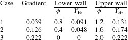
is equal to the increased amount in the upper half-channel. Consequently, the overall reactivity and exothermicity in terms of concentration are held fixed for all cases. A concentration gradient is defined by
 $(Y_{\text{H}_{2},upper}-Y_{\text{H}_{2},lower})/0.036$
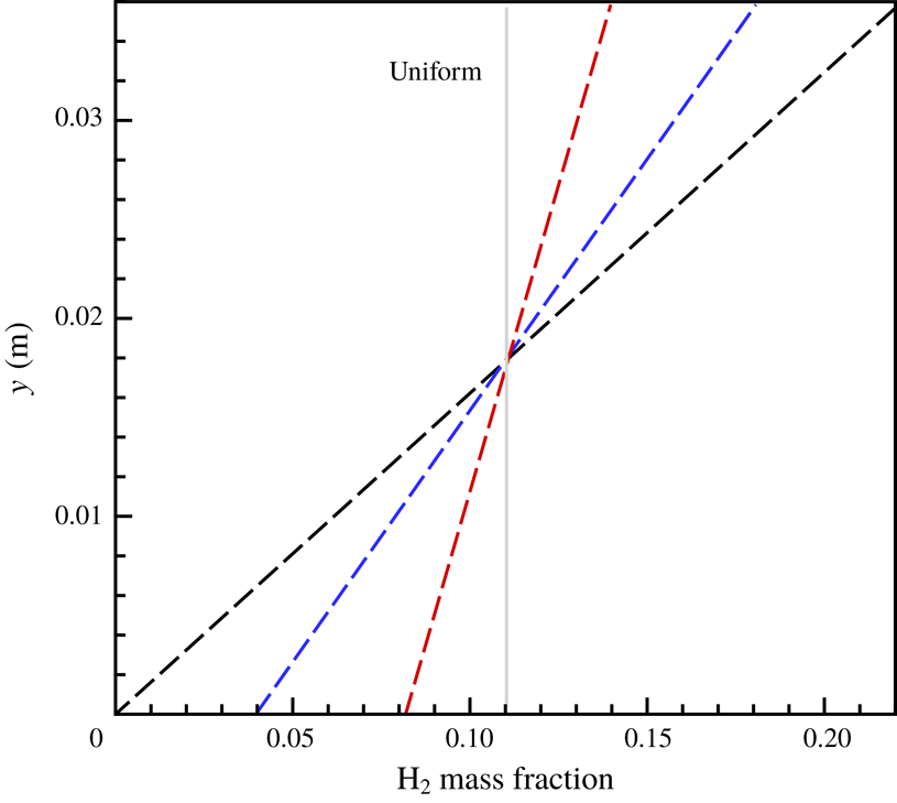
m; and three transversal concentration gradients are given to study systematically the detonation behaviour in the non-homogeneous mixture, as specified in table 1 and shown in figure 1. The simulations were conducted for a constant density of fuel and oxidizer, which permits meaningful comparisons between results with different concentration gradients. While the initial pressure changes slightly as the concentration varies, it is very close to 0.067 atm.
 $\text{H}_{2}$
mass fraction distribution along the transversal direction: red line, Case 1; blue line, Case 2; black line, Case 3.

Transversal concentration gradient.

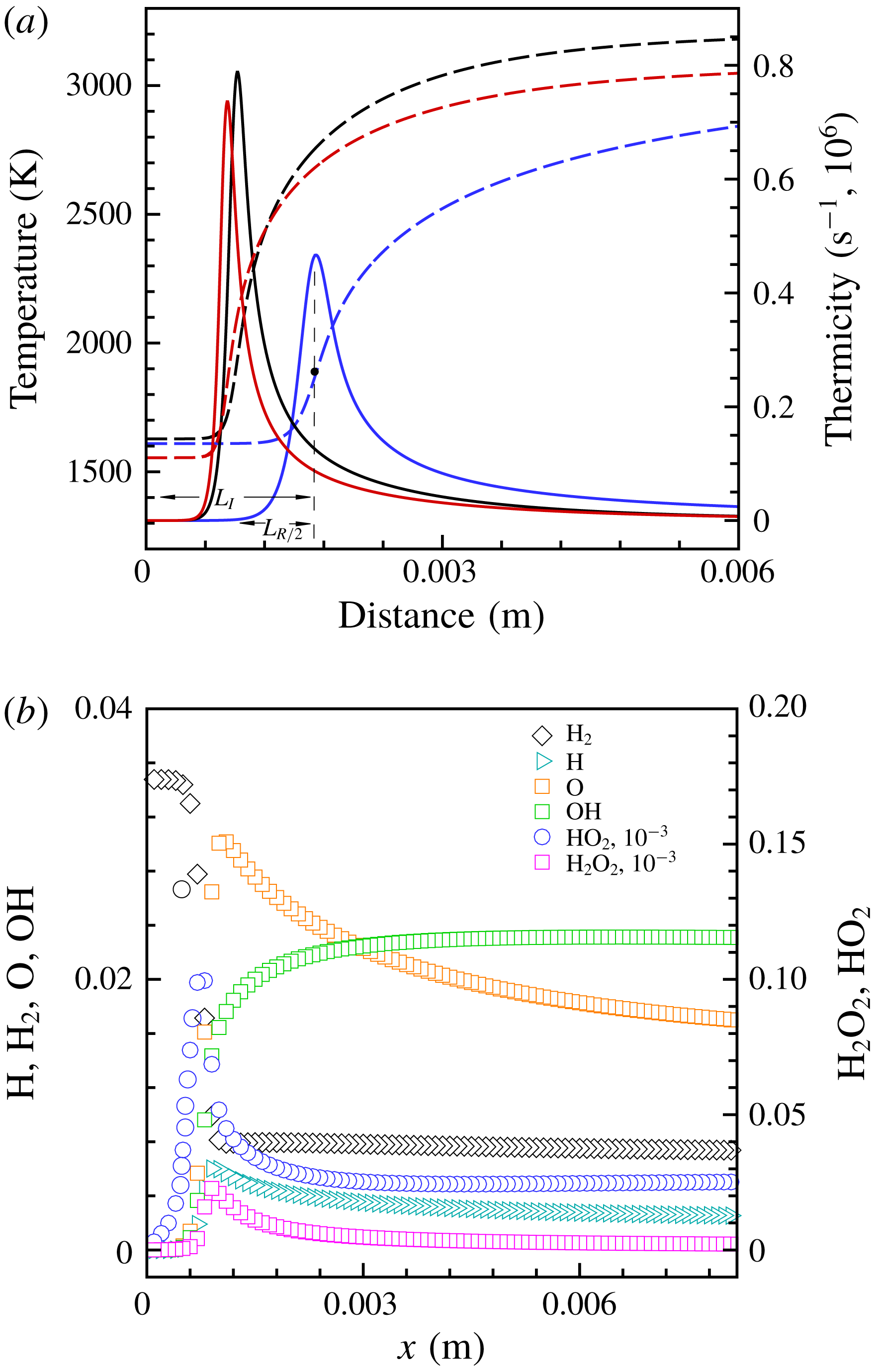
(a) Temperature (dashed line) and thermicity (solid line) profiles of ZND structure for different equivalence ratios (
 $p_{0}=0.067$
atm and
 $T_{0}=300$
K):
 $\unicode[STIX]{x1D719}=0.5$
(red line), 1.0 (black line) and 1.5 (blue line). Here
 $L_{R/2}$
is half of the reaction length and
 $L_{I}$
is the induction length. (b) Species mass fraction for
 $\unicode[STIX]{x1D719}=1.0$
,
 $p_{0}=0.067$
atm and
 $T_{0}=300$
K.

We calculated theoretically the profile of the Zel’dovich–von Neumann–Doering (ZND) structure for the stoichiometric mixture at a pressure of 0.067 atm and a temperature of 300 K, as shown in figure 2. The distance between the maximum temperature gradient and the thermicity position from the shock front is defined as the half-reaction length,
 $L_{R/2}$
, and is
 $6\times 10^{-4}$
m. Three mesh sizes of
 $\unicode[STIX]{x1D6FF}x=2\times 10^{-5}$
,
 $1\times 10^{-5}$
and
 $5\times 10^{-6}$
m were used to simulate two-dimensional detonation in a uniform
 $\text{H}_{2}{-}\text{O}_{2}$
mixture with
 $p_{0}=0.067$
atm and
 $T_{0}=300$
K to verify grid convergence, corresponding grid-resolution levels of, respectively,
 $30~\text{pts}/L_{R/2}$
,
 $60~\text{pts}/L_{R/2}$
and
 $120~\text{pts}/L_{R/2}$
. The profiles of species mass fraction, including
 $\text{H}_{2}$
, H, O, OH,
 $\text{HO}_{2}$
and
 $\text{H}_{2}\text{O}_{2}$
, are given as a reference for the later results; see figure 2(b). It is seen that the sizes of the species consumption and generation layers in the ZND wave are, respectively,
 ${\sim}3\times 10^{-3}$
and
 $3\times 10^{-4}$
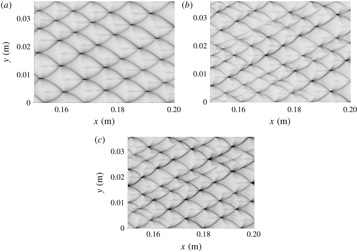
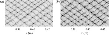
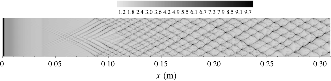
m, and 50 points set in the generation layer of the species is enough to describe the reaction progress. The soot trace is indicated by recording the history of the maximum pressure at each computational cell. Figure 3 shows that for
 $\unicode[STIX]{x1D6FF}x=2\times 10^{-5}$
m the detonation cell is regular, and is significantly different from those obtained with
 $\unicode[STIX]{x1D6FF}x=1\times 10^{-5}$
and
 $5\times 10^{-6}$
m which have similar global features, with almost consistent average cell size. The measured cell size is on average
 ${\sim}0.01$
m, and is comparable to but smaller than the experimental value of
 ${\sim}0.016$
m (Kaneshige & Shepherd Reference Kaneshige and Shepherd1997). Consequently, the grid resolution of
 $\unicode[STIX]{x1D6FF}x=1\times 10^{-5}$
m is capable of describing the cellular detonation propagation and as such is adopted for the present calculations.
Histories of shock pressure for
 $\unicode[STIX]{x1D719}=1$
: (a)
 $2\times 10^{-5}$
m, (b)
 $1\times 10^{-5}$
m, (c)
 $5\times 10^{-6}$
m.

Histories of shock pressure for
 $\unicode[STIX]{x1D719}=0.5$
: (a)
 $1\times 10^{-5}$
m, (b)
 $5\times 10^{-6}$
m.

From figure 2, we observe that for
 $\unicode[STIX]{x1D719}=0.5$
the induction and reaction lengths are close to those of the stoichiometric mixture, while the thermicity is lower than that for
 $\unicode[STIX]{x1D719}=1.0$
. However, for
 $\unicode[STIX]{x1D719}=1.5$
the reaction and induction zones are longer compared with those for
 $\unicode[STIX]{x1D719}=1.0$
. Hence, we carried out a study of grid resolution for the detonation in the fuel-lean mixture with
 $\unicode[STIX]{x1D719}=0.5$
. Figure 4 shows that the results obtained with two levels of
 $1\times 10^{-5}$
and
 $5\times 10^{-6}$
m have globally consistent cell regularity, demonstrating that good convergence of grid resolution is obtained for the fuel-lean detonation and the grid resolution of
 $1\times 10^{-5}$
m is valid for the fuel-lean detonation with
 $\unicode[STIX]{x1D719}=0.5$
. Since the induction and reaction zones are longer for
 $\unicode[STIX]{x1D719}=1.5$
, the grid resolution of
 $1\times 10^{-5}$
m is sufficient to capture the detonation structure in fuel-rich mixtures.
4 Results and discussion
4.1 Global cellular structures for different concentration gradients
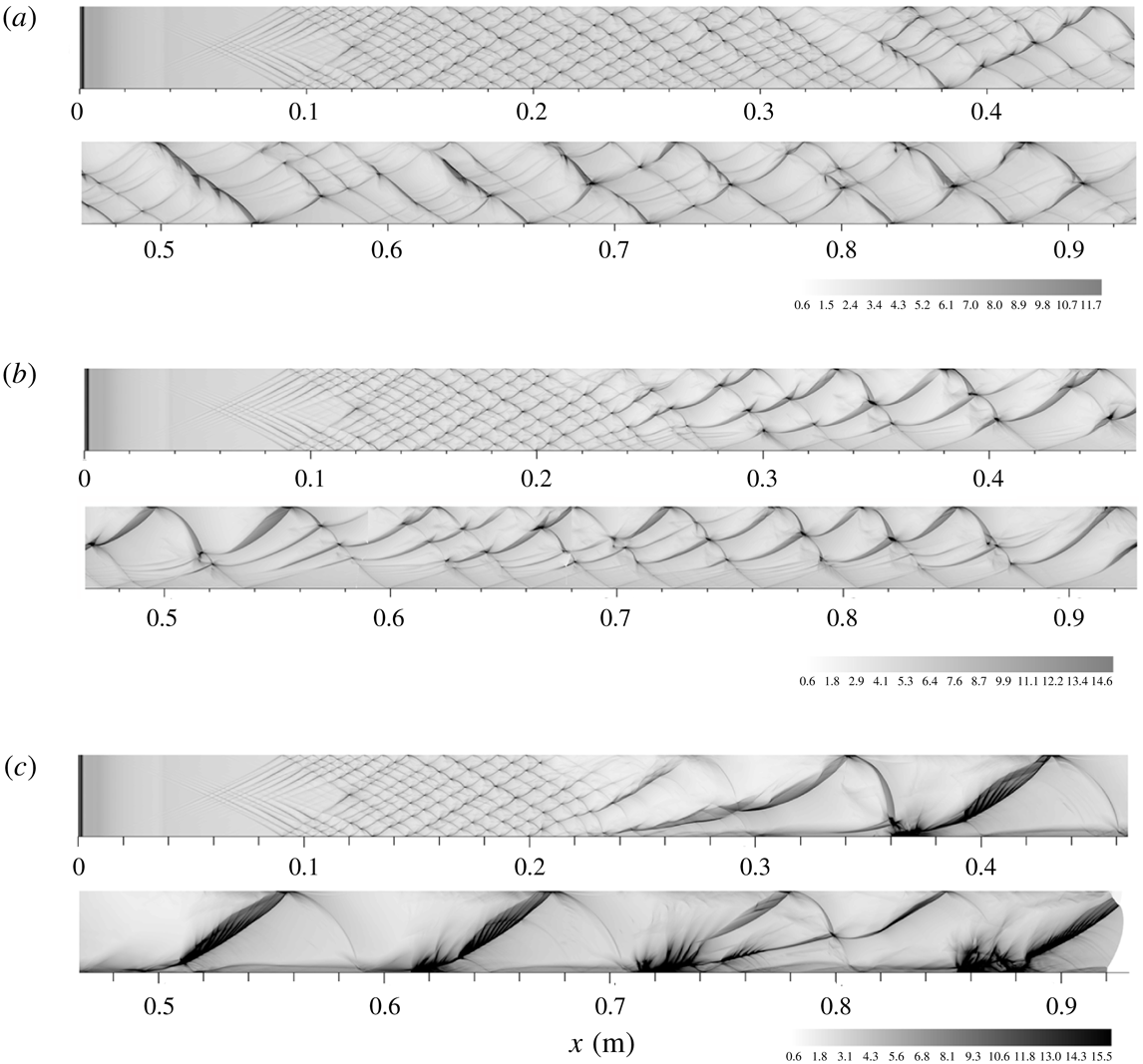
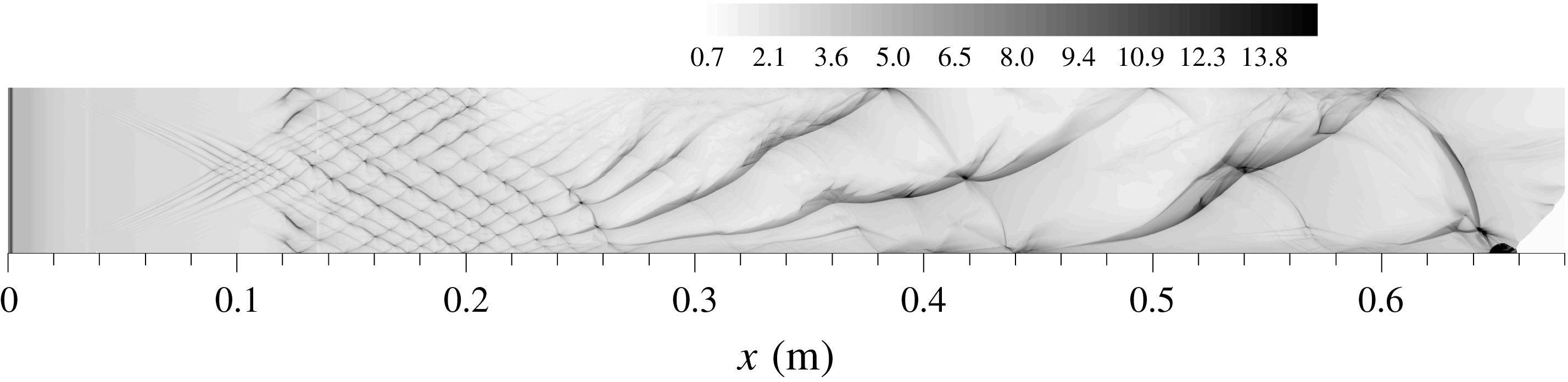
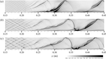
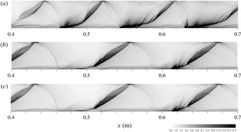
Figure 5 shows the evolution of the cellular structure of the detonation that initially propagates in a uniform mixture and then transits into a non-homogeneous mixture with various transversal concentration gradients. It is seen that while the cellular detonation formed in the uniform region is sustained as it propagates into the non-homogeneous region, cellular instability is enhanced due to the transversal concentration gradient. That is, steepening the concentration gradient not only promotes transition to the irregular cell, it also leads to changes of the detonation mode in the non-homogeneous medium, as shown in figure 5(a–c). It is seen that, with increasing concentration gradient, the detonation cell becomes more irregular while the average cell size also increases in the non-homogeneous region. The cell shape is much distorted, becoming longer and narrower. Based on the global features, the detonation cell can then be classified as: multi-head modes, with either mildly irregular or highly irregular cells, and single-head mode.
Histories of shock pressure: (a) Case 1, (b) Case 2, (c) Case 3.

Specifically, figure 5(a) shows that, for Case 1, the detonation cell in the non-homogeneous region becomes irregular and larger than that in the uniform region. For Case 2, the cell is more irregular than that for Case 1, while the cell size is larger in the fuel-rich layer than in the fuel-lean layer. The cell shape is highly distorted and the ratio of cell length to width is larger. However, for Case 3 only one triple point is left on the front at
 $x\sim 0.3$
m; subsequently the detonation propagates in a single-head mode at
 $x\sim 0.3$
–0.7 m. As a consequence, half of the cell spans the entire channel, resembling the characteristic of highly unstable detonation reported by Radulescu et al. (Reference Radulescu, Sharpe, Law and Lee2007). Furthermore, the thicker tracks are also similar to those observed for near-limit propagation (Gamezo et al.
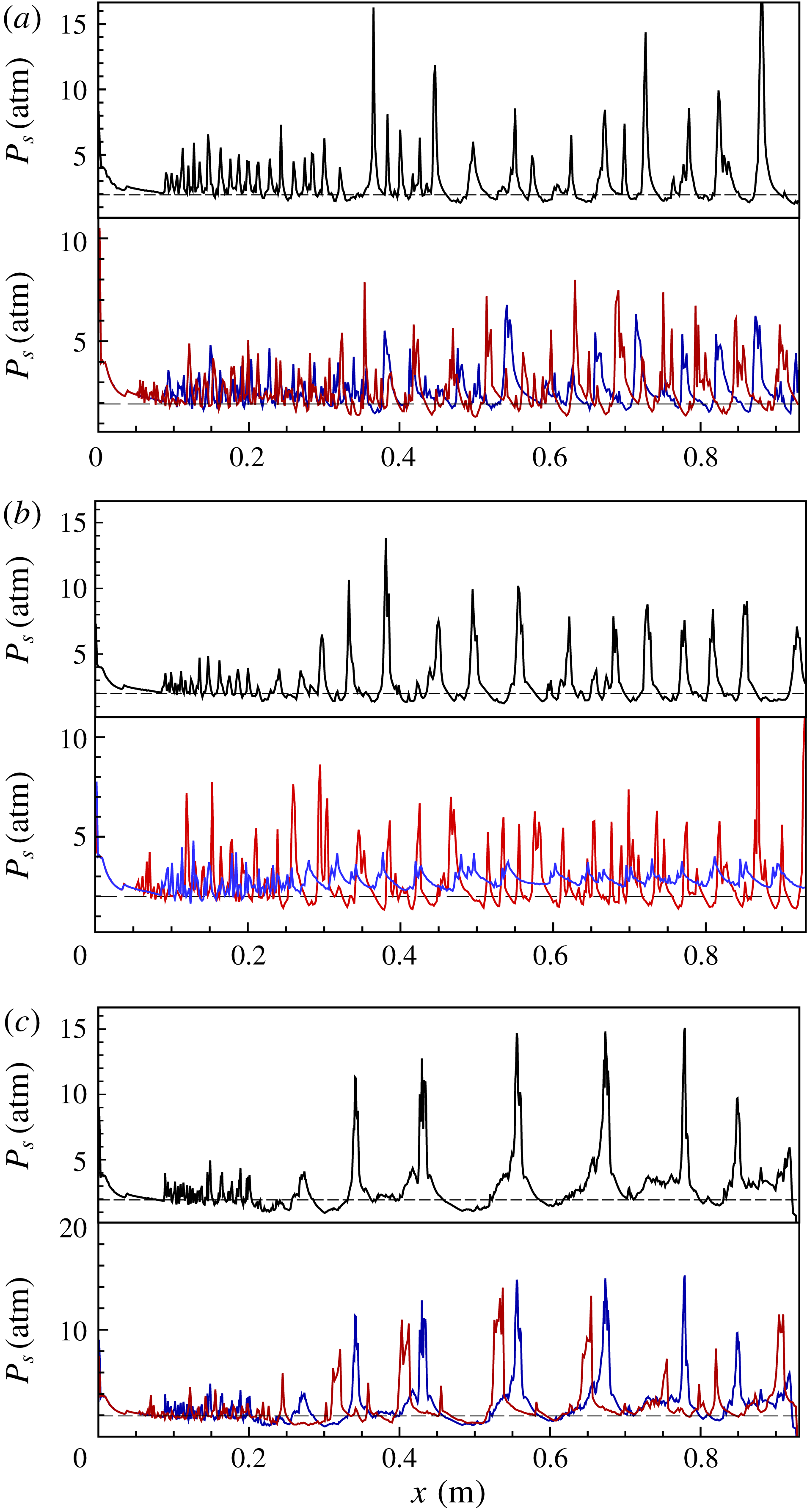
Reference Gamezo, Vasil’v, Khokhlov, Oran and Parvar2000), with finer structures observed in the main tracks, as will be discussed later. The histories of the shock pressure along the lines of
 $y=0$
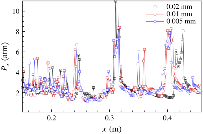
, 18 and 36 mm are shown in figure 6. For these three cases, the oscillation amplitude of the shock pressure increases prominently as the detonation moves into the non-homogeneous regions, while the oscillation frequency is reduced on average, indicating that a concentration gradient leads to locally stronger detonation. It is seen further that steepening the concentration gradient increases the amplitude of the local pressure oscillation.
Histories of shock pressure along lines of
 $y=0$
(blue), 18 (red) and 0.036 m (black): (a) Case 1, (b) Case 2, (c) Case 3.

In summary, a concentration gradient enhances the cellular instability of detonation and causes an increase in the cell size on average, while fuel deficiency does not necessarily reduce the local pressure loads and can actually increase them. Furthermore, steepening the concentration gradient produces stronger local explosions, implying that a detonation running through a mixture with a concentration gradient has a higher destructive potential than that in a homogeneous mixture.
4.2 Frontal structure of detonations for different concentration gradients
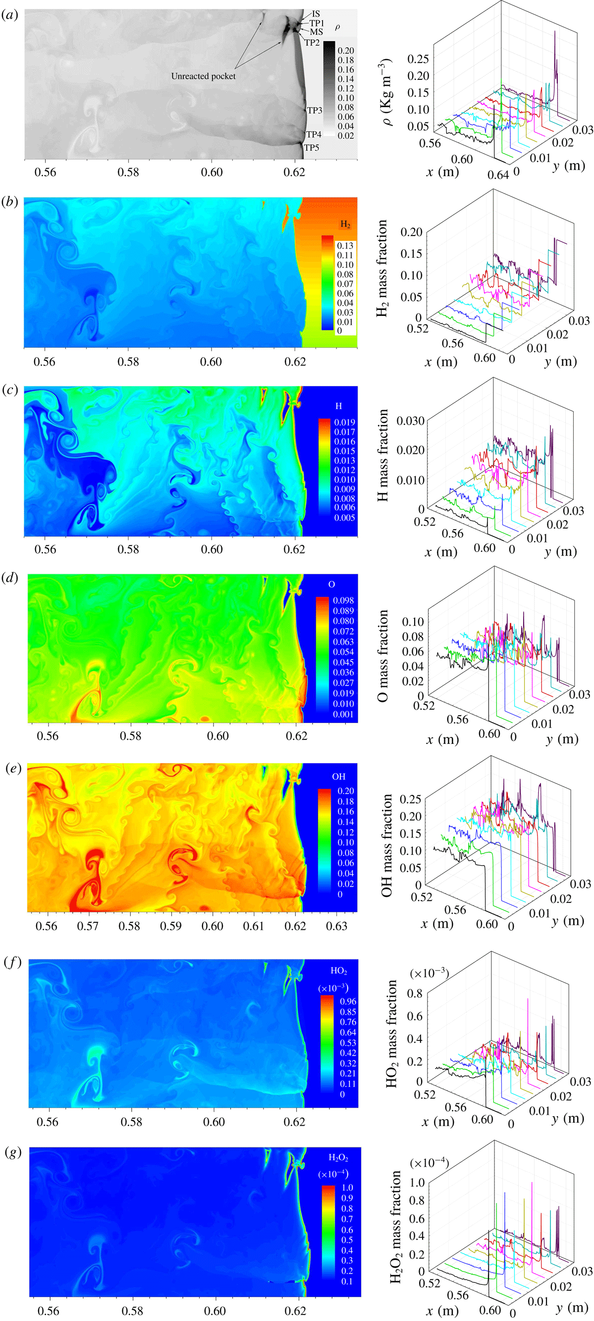
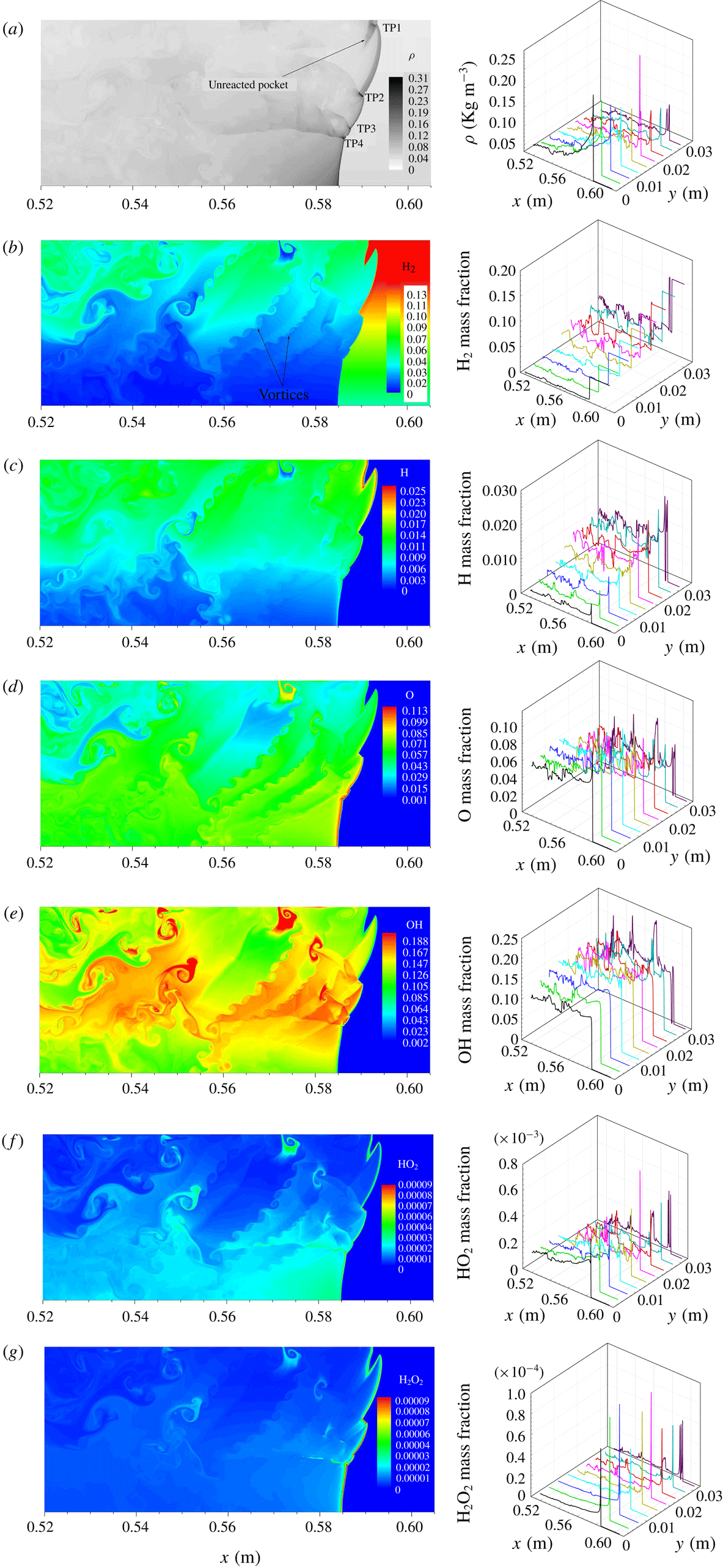
We next study in detail the frontal structure in order to explain the above observation that a concentration gradient enhances cellular detonation instability. Figure 7 shows the frontal structure and species distribution for the detonation wave in Case 1. The frontal feature is similar to that of normal cellular detonation, with a globally thin detonation structure. The fluctuations of the physical variables are small in the downstream flow, demonstrating that reaction and hydrodynamic equilibrium can be reached on average; see figure 7(a). We observe further that the detonation front contains a multi-head structure and, owing to the concentration gradient, the induction zone is thicker in the fuel-rich layer than in the fuel-lean layer, with six triple points on the front. TP1 and TP2 in the fuel-rich layer are stronger than those in the fuel-lean layer, and they collide with each other such that TP1 moves towards the top, while TP2 runs downwards. Note that the
 $\text{H}_{2}$
mass fraction has small humps in the induction zone of the fuel-rich layer due to the interaction of the incident shock with the non-homogeneous gas. More
 $\text{H}_{2}$
in the fuel-rich layer enters the Mach shock front where the reaction time is short behind the collision of triple points. Consequently, an unreacted pocket is left behind the Mach shock, as shown in figure 7(b), with high density of
 ${\sim}0.28~\text{kg}~\text{m}^{-3}$
(
 ${\sim}8.6\unicode[STIX]{x1D70C}_{0}$
). Figure 7(b) shows that the
 $\text{H}_{2}$
mass fractions in the unreacted pocket are equal to those in the upstream state. TP3 and TP4 are relatively weak and move upwards; while TP5 runs downwards, with long tails. As triple points move in the non-homogeneous mixture, vortices are formed behind the detonation front due to the R–M instability. In the fuel-rich layer, the H mass fraction in the frontal structure and at boundary of unreacted pocket is significantly high; see figure 7(c). In the downstream vortex structure, the H mass fraction is also relatively high since the burning rate is increased by the enhancement of mixing of
 $\text{H}_{2}$
and
 $\text{O}_{2}$
left behind the front. The H, O and OH mass fractions all take on strong fluctuations in the downstream flow, indicating that local reaction still continues and chemical equilibrium is not reached locally.
 $\text{HO}_{2}$
and
 $\text{H}_{2}\text{O}_{2}$
concentrate mainly in the detonation front structure and at the triple points; with
 $\text{HO}_{2}$
mass fraction in the front structure being
 ${\sim}0.75\times 10^{-3}$
, while the
 $\text{H}_{2}\text{O}_{2}$
mass fraction is
 ${\sim}1.0\times 10^{-5}$
. They are important for the initiation of induction reactions in the detonation front structure. Moreover, the
 $\text{HO}_{2}$
and
 $\text{H}_{2}\text{O}_{2}$
mass fractions are significantly higher at the boundaries of the unreacted pocket, indicating that they contribute to the induction reaction of the unreacted pocket, as substantiated by the larger local fluctuations of the
 $\text{HO}_{2}$
and
 $\text{H}_{2}\text{O}_{2}$
concentrations downstream. Consequently, satisfactory prediction of the detonation structure as well as unreacted pockets in the non-homogeneous mixture requires a detailed reaction mechanism.
Detonation frontal structures for Case 1 (
 $t=228.27~\unicode[STIX]{x03BC}\text{s}$
): (a) density and (b–g) species mass fraction along lines at different
 $y$
-direction positions (one-dimensional cuts obtained by a increment of 0.4 mm).

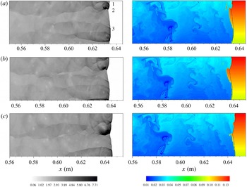
Figure 7 further shows that an unreacted pocket always appears in the fuel-rich layer behind the strong Mach shock caused by the collision of the triple points, and eventually persists downstream. Figure 8 then shows the subsequent consumption of the unreacted pockets and evolution of the detonation frontal structure. Specifically, at
 $t=229.05~\unicode[STIX]{x03BC}\text{s}$
, the unreacted pockets are burnt rapidly, and the
 $\text{H}_{2}$
concentration gradient is slightly reduced in the zone compressed by the incident shock. TP2 runs downwards and consumes the large amount of the
 $\text{H}_{2}$
fuel there. At
 $t=230.46~\unicode[STIX]{x03BC}\text{s}$
, TP1 interacts with the upper wall and the reflected transverse wave is stronger. The resulting Mach shock can directly initiate the gas as the reflection shock runs downwards, while TP6 reflects from the bottom and moves upwards. At
 $t=233.26~\unicode[STIX]{x03BC}\text{s}$
, TP2 collides with TP3 running upwards, leading to strong local explosion and consumption of a large amount of the gas in the compressed zone such that there is no unreacted pocket behind the collision. In summary, detonation with a small concentration gradient behaves similarly to that in the uniform mixture, as is reasonable to expect. The global detonation structure still is relatively thin, with most of the gas entering the front burnt out. This leaves a very low concentration of
 $\text{H}_{2}$
left downstream except for an unreacted pocket appearing in the fuel-rich layer.
Evolution of frontal structures and consumption of unreacted pocket for Case 1: (a)
 $t=229.05$
, (b)
 $230.46$
and (c)
 $233.26~\unicode[STIX]{x03BC}\text{s}$
.

For Case 2, the global detonation front is substantially inclined due to an increase in the concentration gradient, particularly near the bottom. Figure 9 shows that four triple points are on the detonation front, which is fewer than in Case 1. TP1 and TP2 in the fuel-rich layer are stronger than TP4 in the fuel-lean layer. An incident shock forms between TP1 and TP2 and the gas entering the incident shock forms a compressed zone. As TP1 runs upwards, more unreacted gas with concentration gradient enters the front. A bulk unburnt pocket near the upper wall forms after TP1 interacts with it, as shown by the
 $\text{H}_{2}$
mass fraction in figure 9(b). Meanwhile, TP2 runs in the compressed zone, leaving a thick track, as shown in figure 5(b). Figure 9(b) further shows that, since the excess
 $\text{H}_{2}$
cannot be fully consumed in the fuel-rich layer, a large range of
 $\text{H}_{2}$
is left downstream. It is also noted that the downstream
 $\text{H}_{2}$
mass fraction is approximately
 $0.04$
at the middle, while it is higher (
 ${\sim}0.08$
) in the fuel-rich layer. Consequently, about 9 % of the initial
 $\text{H}_{2}$
on average remains downstream. This amount of
 $\text{H}_{2}$
is transported to the region rich in
 $\text{O}_{2}$
and is further reacted. Furthermore, some vortices are created by the R–M instability due to the concentration gradient, hence facilitating mixing of the unreacted
 $\text{H}_{2}$
with
 $\text{O}_{2}$
. Figure 9(c–e) shows that there also exists downstream local reaction where the
 $\text{H}_{2}$
is substantially consumed, producing a considerable amount of OH. From the distribution of the species mass fraction, fluctuations of species in the downstream flow field are stronger than in Case 1. Consequently, chemical and hydrodynamic equilibria are difficult to be attained downstream, which increases effectively the average hydrodynamic thickness. Similar to Case 1,
 $\text{HO}_{2}$
and
 $\text{H}_{2}\text{O}_{2}$
appear mainly in the leading front of the main reaction layer. While the
 $\text{HO}_{2}$
concentration still is close to that in Case 1, the maximum
 $\text{H}_{2}\text{O}_{2}$
mass fraction is
 ${\sim}0.88\times 10^{-4}$
and is higher than that in Case 1; see figure 9(f,g). Consequently,
 $\text{H}_{2}\text{O}_{2}$
is more important for the global propagation in the steepened concentration gradient in comparison to Case 1.
Frontal structure and species distribution for Case 2 (
 $t=217.89~\unicode[STIX]{x03BC}\text{s}$
): (a) density and (b–g) species mass fraction.

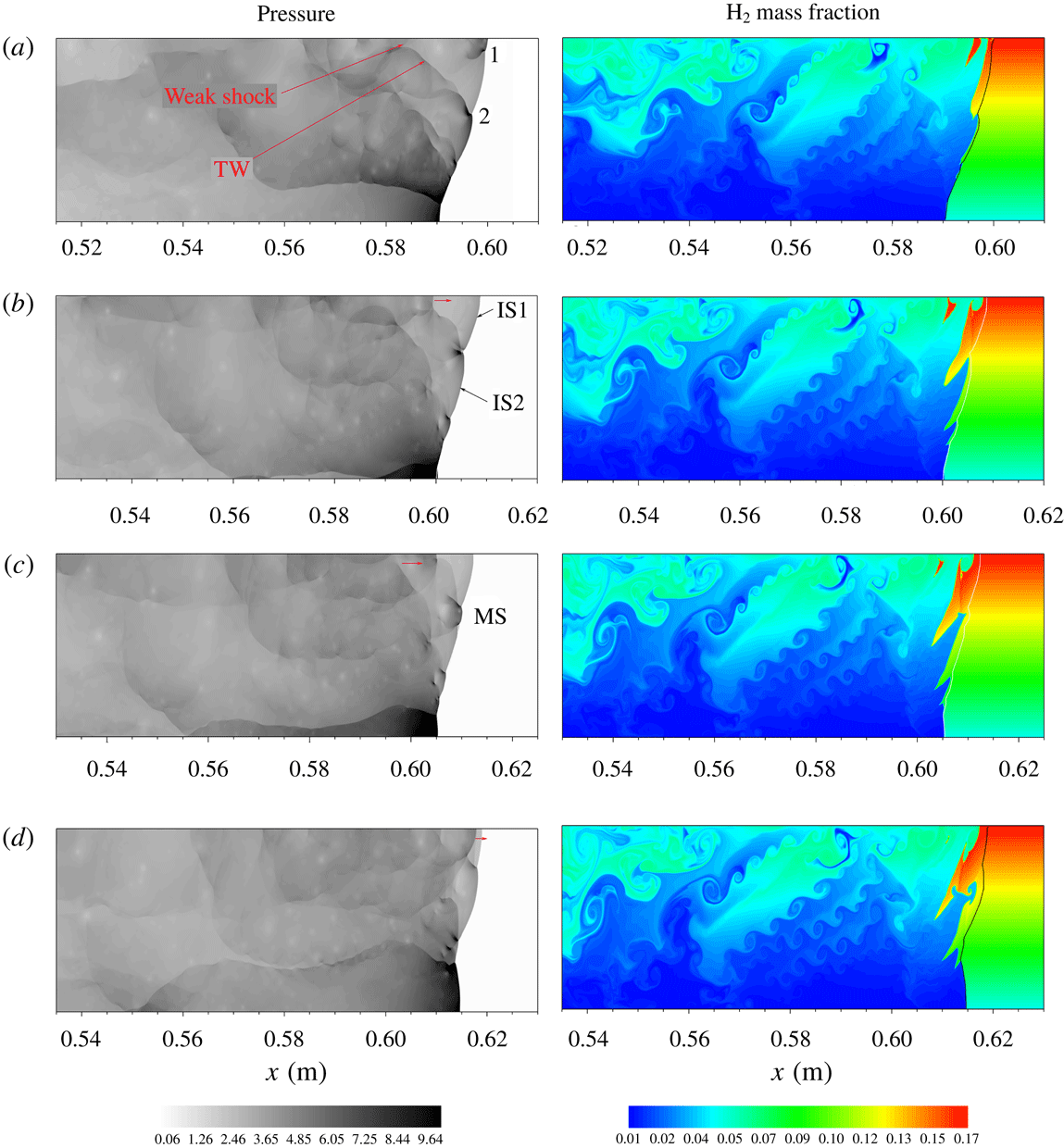
Similar to Case 1, an unreacted pocket appears in the fuel-rich layer, as shown in figure 9(b). Figure 10 shows the subsequent evolution of the front structure and consumption of the unreacted pocket. At
 $t=220.1~\unicode[STIX]{x03BC}\text{s}$
, TP1 runs downwards and a strong Mach shock forms near the upper wall, while TP2 constantly moves upwards along the inclined front. As TP1 runs downwards and decays, the Mach shock also decays to an incident shock (IS1), and reaction of the gas entering the IS1 front is significantly delayed. Meanwhile, as TP2 moves upward into the fuel-rich zone,
 $\text{H}_{2}$
escapes from the initiation by TP2 into the slip layer. At
 $t=223.5~\unicode[STIX]{x03BC}\text{s}$
, TP1 collides with TP2, and subsequently move opposite at
 $t=225.5~\unicode[STIX]{x03BC}\text{s}$
. As the resulting Mach shock decays, the gas entering its front is not initiated immediately at
 $t=225.5~\unicode[STIX]{x03BC}\text{s}$
and the bulk of unreacted gas remains behind the IS1 and IS2 fronts in the fuel-rich layer; see figure 10(c,d). Furthermore, a weak shock appears downstream near the top and a curved transverse wave tails TP2, as shown in figure 10(a,b). The transverse shock is reflected by the upper wall and then interacts with and strengthens the downstream shock near it. Moreover, the shock is also reinforced by the heat release of the unreacted pocket so that it can catch up with and strengthen IS1, as shown in figure 10(d). However, although the strengthened IS1 slightly enhances the reaction rate of the gas behind it, substantial unreacted
 $\text{H}_{2}$
remains behind IS1 since the ignition delay time in the very rich
 $\text{H}_{2}$
region is rather long. Consequently, when SP1 reaches the upper wall and is reflected again, new unreacted pockets near the upper wall are formed.
Evolution of triple point and consumption of unreacted pocket for Case 2: (a)
 $t=220.1~\unicode[STIX]{x03BC}\text{s}$
, (b) 223.5, (c) 225.2, (d) 228.7 and (e)
 $230.5~\unicode[STIX]{x03BC}\text{s}$
.

Instantaneous temperature contour (a) in figure 10(a);
 $\text{H}_{2}$
(b),
 $\text{O}_{2}$
(c) mass fraction along lines 1–3; longitudinal (d) and transversal (e) laboratory frame particle velocity,
 $\text{H}_{2}$
(f) and
 $\text{O}_{2}$
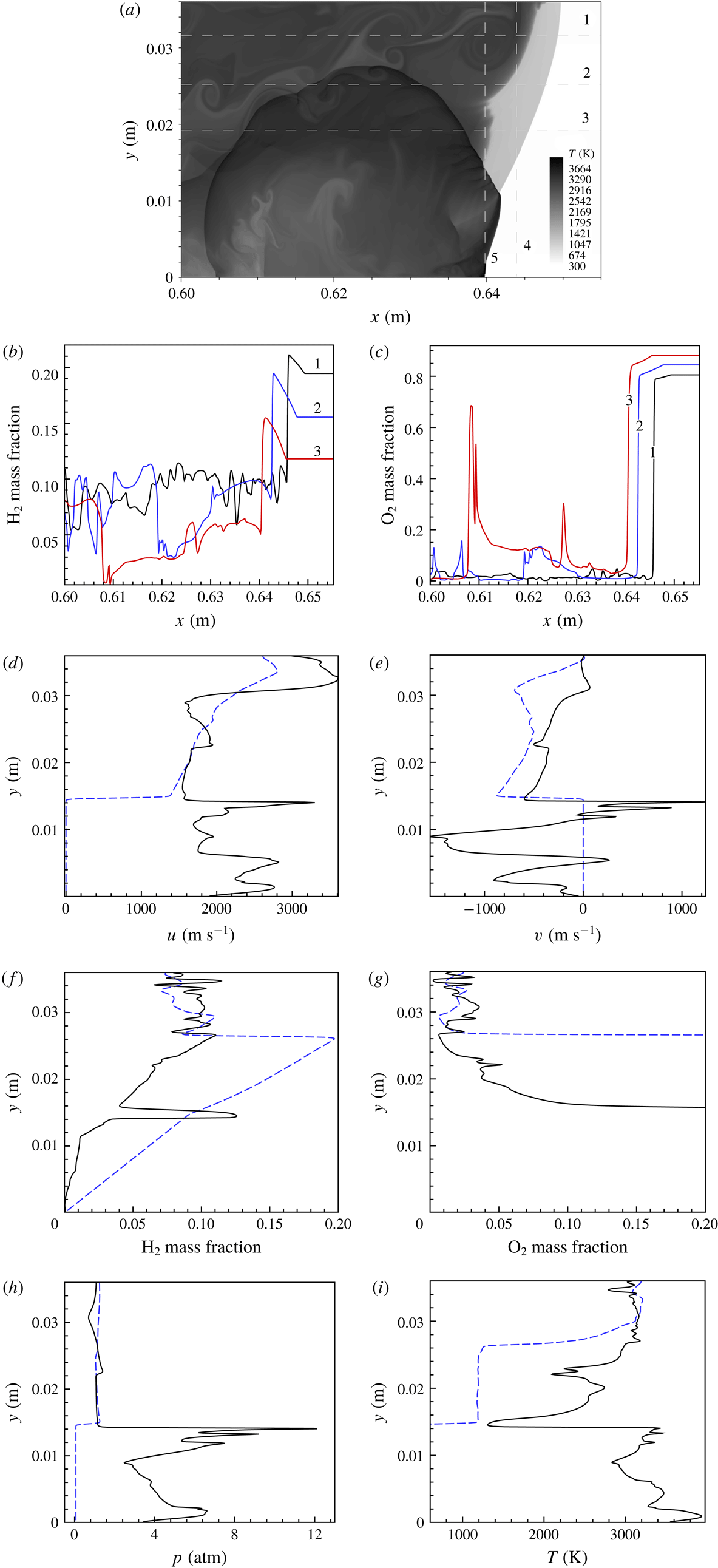
(g) mass fraction, pressure (h) and temperature (i) along lines 4 and 5; lines 1–5 are one-dimensional cuts of the flow field of (a).

We have further analysed the local details of the flow field to reveal how they affect the ignition delays of the processed gas. Figure 11 shows the
 $\text{H}_{2}$
and
 $\text{O}_{2}$
profiles along lines 1–3 and the pressure, temperature, velocity and
 $\text{H}_{2}$
and
 $\text{O}_{2}$
mass fraction profiles along lines 4 and 5. It is seen that the
 $\text{H}_{2}$
mass fraction in the unreacted pocket is equal to that in initial upstream, indicating that
 $\text{H}_{2}$
in the unreacted pocket is not completely consumed. It is of interest to note that in the zone compressed by IS1 and IS2, the
 $\text{H}_{2}$
mass fraction takes on obvious humps, while the
 $\text{O}_{2}$
mass fraction slightly decreases; see the black and blue lines in figure 11(b,c). This is reasonable because the inclined IS1 sweeps the gas with concentration gradient so that
 $\text{H}_{2}$
in the richer layer flows to the region with relatively lower
 $\text{H}_{2}$
concentration, which is also substantiated by the transversal flow direction in the compressed zone behind IS1; see the blue line in figure 11(e). The interaction of the leading shock with the mixture increases the inhomogeneity of the local mixture, leading to the hump of
 $\text{H}_{2}$
. The excess
 $\text{H}_{2}$
in the compressed zone is left and forms an unreacted pocket behind the shock front. The leading shock in a non-homogeneous mixture plays the dual role of inducing the reaction as well as enhancing local inhomogeneity and local concentration gradient increases (see the blue lines in figure 11
f,g), which is origin of the unreacted pocket.
Before the unreacted pocket appears at right, we take out the temperature and pressure of the shocked gas in front of the pocket at
 $y=0.028$
m (
 $\unicode[STIX]{x1D719}=1.11$
) in figure 7. The local pressure and temperature of the shocked gas in front of the unreacted pocket are, respectively,
 ${\sim}1.15$
atm and 1128 K and thus the corresponding ignition delay time is
 ${\sim}t_{N}=26~\unicode[STIX]{x03BC}\text{s}$
. The average length of the unreacted pocket in figure 7 is
 ${\sim}3\times 10^{-4}$
m. The numerical flame speed is measured by tracking the effective dimension of the unreacted pocket at these two times and can be calculated by
 $\boldsymbol{U}_{f}=(L_{p,t_{1}}-L_{p,t_{2}})/(t_{2}-t_{1})$
, where
 $L_{p,t_{1}}$
and
 $L_{p,t_{2}}$
are, respectively, the effective dimensions of the pockets at
 $t_{1}$
and
 $t_{2}$
. The average flame speed is
 ${\sim}128~\text{m}~\text{s}^{-1}$
for the pocket in figure 7. Hence, the distance it takes for the pocket to be consumed due to autoignition through shock compression is estimated as
 ${\sim}\boldsymbol{U}_{f}t_{N}=3.3\times 10^{-3}$
m, which is much larger than the dimension of the pocket actually observed in figure 7. For Case 2, figure 11(h,i) shows the temperature and pressure profiles illustrating the position of the unreacted highly compressed and cool gases undergoing ignition. It is seen that in the compressed zone behind IS1, the pressure peak is
 ${\sim}2.2$
atm, which is slightly higher than the von Neumann value of 1.98 atm in the stoichiometric mixture, and the shocked temperature is
 ${\sim}1000$
K. The distance calculated by the ignition delay time is
 ${\sim}5.8\times 10^{-3}$
m at
 $y=0.034$
m (
 $\unicode[STIX]{x1D719}=1.15$
,
 $p_{N}=1.17$
atm,
 $T_{N}=1126$
K; the ignition delay time is
 $8.9~\unicode[STIX]{x03BC}\text{s}$
), which is much larger than the dimension of the pocket of
 ${\sim}0.8$
mm, shown in figure 7. Consequently, it is identified that the unreacted pocket is burnt through surface reactions and the numerical viscosity plays a role in burning the pocket.
Evolution of triple point for Case 3: (a)
 $t=202.25$
, (b) 216.08, (c) 225.4 and (d)
 $231.2~\unicode[STIX]{x03BC}\text{s}$
.

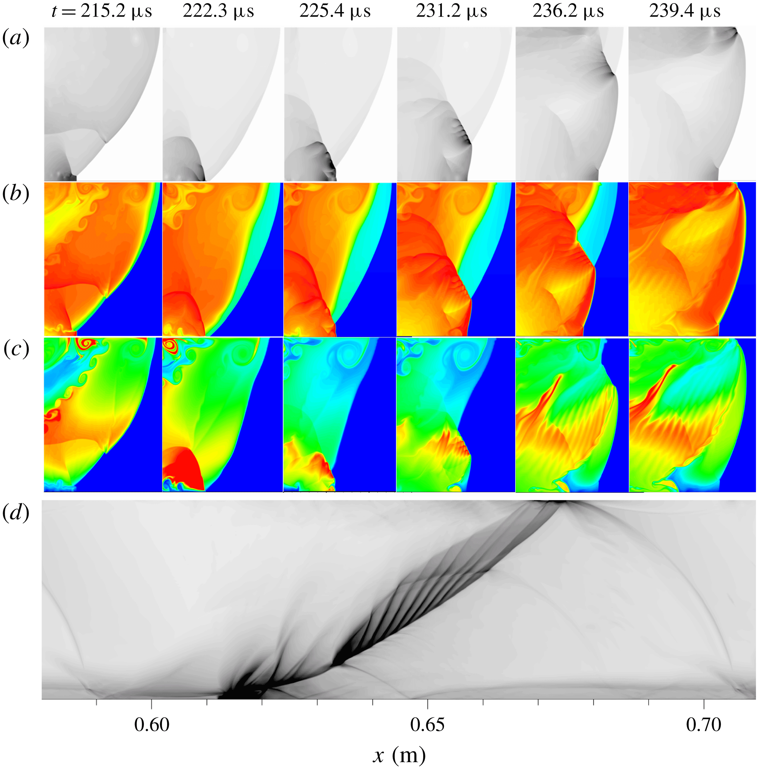
For Case 3, the detonation takes on a single-head mode and only one triple point is present at the front. Figure 12 shows the evolution of the triple point during one period. It is seen that the inclination of the detonation front is further amplified, while the global detonation structure thickens. At
 $t=202.25~\unicode[STIX]{x03BC}\text{s}$
, the detonation front consists of the Mach shock near the top, and incident shock and Mach stem near the bottom. The triple point moves downwards and a strong Mach shock forms near the top, with an eddy behind the Mach shock front. The Mach shock initiates the
 $\text{H}_{2}$
in the fuel-rich layer near the upper wall, with complicated transverse waves propagating downwards. There is no bulk unreacted pocket left downstream, while the excess
 $\text{H}_{2}$
behind the Mach shock and incident shock fronts appears downstream in the fuel-rich layer and forms the remaining
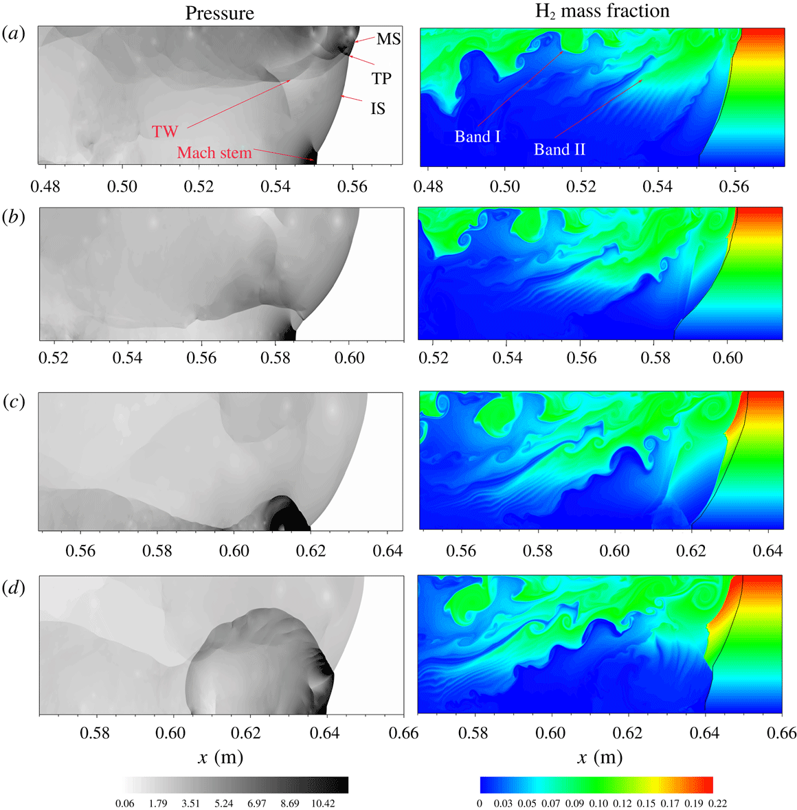
 $\text{H}_{2}$
band, with some vortices caused by the R–M instability at the boundaries of the band. Meanwhile, the unreacted
 $\text{H}_{2}$
band near the top extends far downstream. At that instant, the incident shock still couples with the reaction zone; see the right-hand panel in figure 12(a). As the triple point moves downwards, the Mach shock decays constantly. At
 $t=216.08~\unicode[STIX]{x03BC}\text{s}$
, a small amount of the gas entering its front is reacted, and the unreacted
 $\text{H}_{2}$
band extends to the fuel-lean layer and far downstream due to the interaction of the transverse wave moving downwards; see figure 12(b). Consequently, in the far-downstream flow field the remaining
 $\text{H}_{2}$
reacts constantly and is consumed substantially, and species mass fractions take on strongly local fluctuations, as shown in figure 15. Meanwhile, the front is highly inclined and a Mach stem forms near the bottom to match with the wall boundary condition. At
 $t=225.4~\unicode[STIX]{x03BC}\text{s}$
, the triple point interacts with the gas compressed by the Mach stem and collides with the lower wall, leading to strong local explosion near the lower wall. At that instant, the incident shock decays further and more gas behind it is not initiated such that a compressed zone forms behind it; see figure 12(c,d). The explosion wave develops forward to the Mach shock, while it evolves to a transverse detonation and propagates in the compressed zone, with fine structure in the transverse detonation front; see figure 12(d). As the transverse detonation moves into the compressed zone, the compressed gas is initiated and
 $\text{H}_{2}$
is substantially consumed, with the remaining
 $\text{H}_{2}$
forming a new band, similar to that in figure 12(a). Furthermore, the transverse wave is also reflected from the lower wall and propagates towards the upper wall, as shown in figure 12(c). At
 $t=231.2~\unicode[STIX]{x03BC}\text{s}$
, the reflected transverse wave interacts with the extended band of unreacted
 $\text{H}_{2}$
, which enhances mixing of the remaining
 $\text{H}_{2}$
with
 $\text{O}_{2}$
in the fuel-lean layer and promotes the consumption of the
 $\text{H}_{2}$
fuel downstream. Due to the interaction of the transverse wave, the particle in the band flows towards the top. As the transverse wave steadily propagates upwards, it sweeps the unreacted
 $\text{O}_{2}$
into band I where
 $\text{H}_{2}$
is substantially consumed. Eventually, the remaining
 $\text{H}_{2}$
near the top still is not burnt due to the lack of
 $\text{O}_{2}$
and forms band II that extends far downstream, as shown in figure 12(a). For a uniform
 $\text{H}_{2}{-}\text{O}_{2}$
mixture at
 $p=0.067$
atm and
 $T_{0}=300$
K, the detonation cell size in the stoichiometric mixture is
 ${\sim}0.016$
m, as given in Kaneshige & Shepherd (Reference Kaneshige and Shepherd1997). Consequently, the critical detonation limit corresponds to a critical diameter of
 ${\sim}\unicode[STIX]{x1D706}/3.14=0.005$
m, where
 $\unicode[STIX]{x1D706}$
is the cell size. The present channel width is 0.036 m and it is far from the critical detonation limit, permitting the sustaining of cellular detonation, as substantiated by the detonation behaviour in the uniform region. However, for Case 3 the single-head mode demonstrates that on average the cell size may be close to
 $3.14d$
, showing that the concentration gradient increases the critical diameter to detonation limit. The explosion limits of quiescent
 $\text{H}_{2}{-}\text{O}_{2}$
mixture are in the range of equivalence ratio
 $\unicode[STIX]{x1D719}\sim 0.12$
–4.0 by the theoretical prediction of Wang & Law (Reference Wang and Law2013), showing that the pure
 $\text{H}_{2}{-}\text{O}_{2}$
system has a very wide range of explosivity in the temperature–pressure plane. With a smaller molar fraction of
 $\text{H}_{2}$
, which implies a correspondingly larger molar fraction of
 $\text{O}_{2}$
, the
 $\text{H}_{2}{-}\text{O}_{2}$
system is more explosive near the first limit and less explosive near the third limit. Furthermore, flammability limits for this
 $\text{H}_{2}{-}\text{O}_{2}$
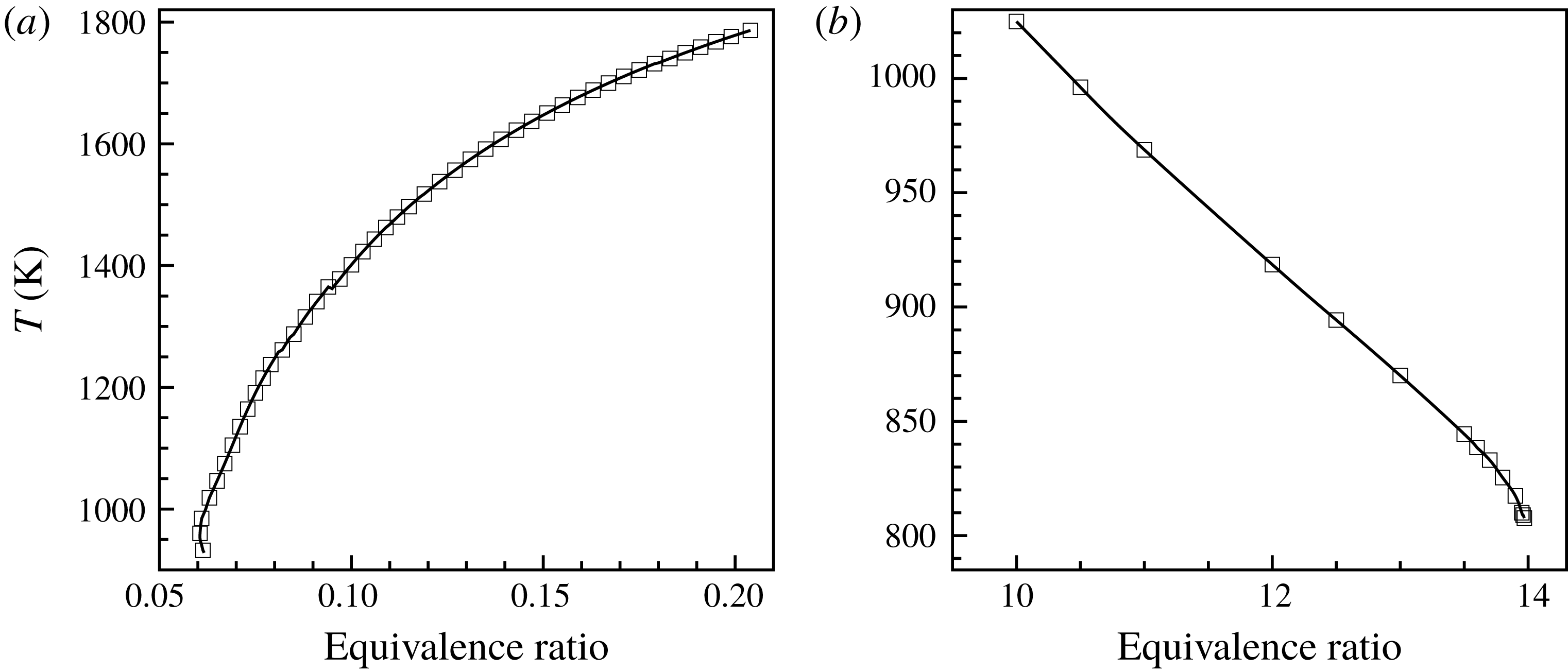
mixture are calculated through considering the radiative heat loss in Ju et al. (Reference Ju, Guo, Kaoru and Liu1997, Reference Ju, Guo, Liu and Kaoru1999). Figure 13 shows the flammability limits for the
 $\text{H}_{2}{-}\text{O}_{2}$
mixture through the flame temperature as a function of the equivalence ratio. It is seen that the lean flammability limit appears at
 $\unicode[STIX]{x1D719}\sim 0.06$
, while the rich flammability limit is at
 $\unicode[STIX]{x1D719}\sim 14$
. The equivalence ratios of
 $\unicode[STIX]{x1D719}=0.06$
and 0.12 are, respectively, at
 $y=0.001$
and 0.002 m of the channel, where the mixture is combustible. Hence, it is reasonable that the reactions occur in the region
 $y\sim 0$
–0.002 m. In addition, convection of the fuel into this region by the travelling transverse waves along and behind the front promotes the occurrence of the local explosion near the bottom wall. This is explained next.
Flammability limits for
 $\text{H}_{2}{-}\text{O}_{2}$
system at
 $p=0.067$
atm and
 $T_{0}=300$
K: (a) fuel-lean regime and (b) fuel-rich regime.

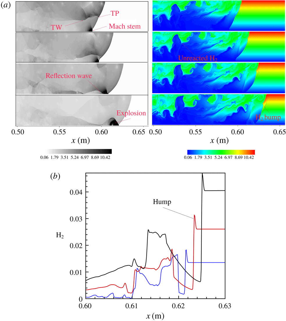
Figure 14 shows the interaction of the leading shock and transverse wave with the
 $\text{H}_{2}$
fuel, showing that there is a transport of the fuel into this region by the travelling transverse waves. At
 $t=211.8~\unicode[STIX]{x03BC}\text{s}$
, the globally inclined shock front forms, with Mach stem near the bottom wall and a main triple point followed by a long transverse wave. While the Mach stem is strong, with the pressure and temperature being, respectively,
 ${\sim}8.2$
atm and 1400 K, no local explosion is observed in the region of
 $y\leqslant 0.002$
m. As the triple point runs downwards, the transverse wave sweeps the fuel in the richer layer into the leaner region. At
 $t=225.4~\unicode[STIX]{x03BC}\text{s}$
, the triple point and transverse wave collide with the bottom wall, leading to strongly local explosion near the bottom. To identify clearly the convection of the fuel into this region, we show the profiles of the
 $\text{H}_{2}$
mass fraction along cuts of
 $y=0.0066$
, 0.0043 and 0.002 m at
 $t=225.4~\unicode[STIX]{x03BC}\text{s}$
in figure 14. It is seen that a hump appears in the profile and the
 $\text{H}_{2}$
mass fraction behind the front is higher than the initial value (see blue line in figure 14
b), indicating that the
 $\text{H}_{2}$
fuel indeed is convected into the fuel-lean layer due to interaction of the leading shock with the gradient.
Evolution of triple point for Case 3. (a) Pressure and
 $\text{H}_{2}$
mass fraction:
 $t=211.8$
, 216.08, 220.3 and
 $225.6~\unicode[STIX]{x03BC}\text{s}$
. (b) Profiles of
 $\text{H}_{2}$
mass fraction.

Frontal structure and species distribution for Case 3 (
 $t=243.46~\unicode[STIX]{x03BC}\text{s}$
): (a) density and (b–g) species mass fraction along lines at different
 $y$
-direction positions.

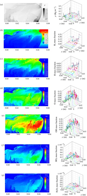
Figure 15 shows the instantaneous front structure and the distribution of species at
 $t=243.46~\unicode[STIX]{x03BC}\text{s}$
. The strong transverse detonation moves towards the top, with fine structure, and the main triple point on the front consists of the transverse detonation, incident shock and Mach shock. As the main triple point moves obliquely upwards, some vortices in the contact surface are produced by the R–M instability and promote mixing of
 $\text{H}_{2}$
and
 $\text{O}_{2}$
behind the front. Consequently, local explosion occurs in the downstream vortices behind the Mach stem near the bottom, substantiated by high OH concentration in figure 15(c–e). For the single-head detonation, the strong transverse detonation propagating from the fuel-lean to fuel-rich layer efficiently consumes the fuel in the compressed zone, shown in figure 15. The local
 $\text{H}_{2}$
concentration in the fuel-rich region is increased by the inclined and curved incident shock and here the local concentration gradient increases, as indicated by obvious humps in the
 $\text{H}_{2}$
mass fraction profile in the fuel-rich region of the right-hand panel in figure 15(c). However, bulk unreacted pockets are not observed behind the detonation front due to the existence of the transverse detonation. The transverse detonation in the single-head detonation propagating in the non-homogeneous mixture is different from the transverse wave in the homogeneous mixture, in that its existence is caused by the transversal concentration gradient, as observed experimentally in Boeck et al. (Reference Boeck, Berger, Hasslberger and Sattelmayer2016), and becomes stronger with steepening of the transversal concentration gradient. As the transverse detonation moves towards the top, the Mach shock front is inclined considerably so that a short Mach stem is formed near the bottom to match the boundary condition. The concentrations of H, OH and O behind the Mach stem are low, indicating that substantial reactions do not occur here because the combustible limit is out near the lower wall. It is further seen that at the transverse detonation front, the maximum
 $\text{HO}_{2}$
and
 $\text{H}_{2}\text{O}_{2}$
mass fractions are higher than those in the other cases, indicating that they play a key role in the transverse detonation, shown in figure 15(f,g). This is reasonable because autoignition in the mixture at high pressures is closely related to the reactions involving
 $\text{HO}_{2}$
and
 $\text{H}_{2}\text{O}_{2}$
(Sánchez & Williams Reference Sánchez and Williams2014). Although there is no bulk unreacted pocket appearing behind the front, a large amount of
 $\text{H}_{2}$
is left downstream in the fuel-rich layer and continues reacting, and meanwhile H, O, OH,
 $\text{HO}_{2}$
and
 $\text{H}_{2}\text{O}_{2}$
all present strong fluctuations downstream; see the right-hand panel of figure 15(c–g). We have found that 18 % of the total
 $\text{H}_{2}$
remains unreacted downstream, in the range of
 $0.52~\text{m}\leqslant x\leqslant 0.56~\text{m}$
. Hence, reaction equilibrium requires a greater distance than in the other two cases, which will be further discussed later.
Instantaneous temperature contour (a) in figure 12(d);
 $\text{H}_{2}$
(b),
 $\text{O}_{2}$
(c) mass fraction along lines 1–3; longitudinal (d) and transversal (e) laboratory frame particle velocity,
 $\text{H}_{2}$
(f) and
 $\text{O}_{2}$
(g) mass fraction, pressure (h) and temperature (i) along lines 4 and 5; lines 1–5 are one-dimensional cuts of the flow field of (a).

Figure 16 shows the
 $\text{H}_{2}$
and
 $\text{O}_{2}$
profiles along lines 1–3 and the pressure, temperature, velocity and
 $\text{H}_{2}$
and
 $\text{O}_{2}$
mass fraction profiles along lines 4 and 5 in one-dimensional cuts. From figure 16(b,c), it is noted that in the compressed zone the
 $\text{H}_{2}$
mass fraction takes on obvious hump, while the
 $\text{O}_{2}$
mass fraction decreases, as compared to that in the initial upstream field. It is also seen that the particle flow in the compressed zone behind the incident shock has negative transversal velocity since the inclined and curved incident shock sweeps the gas with concentration gradient; see the blue line in figure 16(e). Hence,
 $\text{H}_{2}$
in the rich layer flows to the region with lower
 $\text{H}_{2}$
concentration, leading to an enhancement of the local
 $\text{H}_{2}$
concentration and a reduction of the local
 $\text{O}_{2}$
concentrations (see figure 16
f,g), although the global concentration gradient is reduced by the incident shock. The pressure and temperature in the compressed zone are
 ${\sim}1.8$
atm and
 ${\sim}1000$
K, respectively. Hence, the induction time is shortened significantly in the compressed and preheated zones. The transverse detonation can rapidly consume the mixture and propagates obliquely upwards so that the bulk of the unreacted pocket is not observed in Case 3. However, the excess
 $\text{H}_{2}$
from the hump in the fuel-rich layer is left and forms unreacted gas bands, as shown in figure 12. Furthermore, downstream the jump of the
 $\text{O}_{2}$
mass fraction along line 3 indicates that the transverse wave can sweep
 $\text{O}_{2}$
in the fuel-lean layer into the fuel-rich layer and promotes mixing of the remaining
 $\text{H}_{2}$
and
 $\text{O}_{2}$
. Although the residue
 $\text{H}_{2}$
bands are promoted by the transverse waves, they significantly delay achieving chemical equilibrium in the downstream flow. Figure 16(e) further shows that the flow behind the transverse detonation front has negative transversal velocity with a minimum value of
 ${\sim}-1500~\text{m}~\text{s}^{-1}$
, which is preceded by the refraction wave from the lower wall, as shown in figure 16(h).
In summary, the transversal concentration gradient enhances the cellular instability of detonation. Steepening the concentration gradient considerably reduces the number of triple points on the front and lengthens the global detonation front structure on average, leading to more
 $\text{H}_{2}$
fuel left behind it. Nevertheless, the transverse detonation efficiently consumes the fuel and hence the bulk of unreacted pocket does not appear behind the detonation front in Case 3. Due to the steepened concentration gradient, a large amount of unreacted
 $\text{H}_{2}$
remains downstream and strengthens significantly the fluctuation of the species, leading to rather slow attainment of reaction equilibrium. Consequently, the deficit of the average detonation velocity may be increased, to be further discussed next.
4.3 The front dynamics
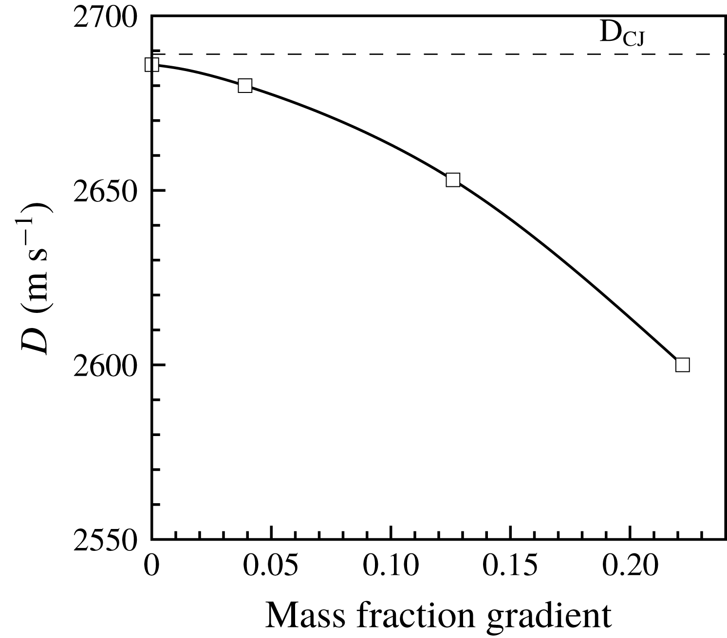
The above discussions have demonstrated that the concentration gradient enhances cellular instability and leads to the transition from multi-head mode to single-head mode. Figure 17 shows the average detonation velocity as a function of concentration gradient, with the average velocity determined by calculating the ratio of the distance difference between two average shock positions, which is obtained by integrating across the entire channel front to the corresponding time difference. It is seen that a concentration gradient leads to a deficit of the average velocity, as compared with that in the uniform mixture, steepening the concentration gradient leading to increased deficit. For Case 1, the average velocity is approximately close to the CJ value; while it is
 ${\sim}0.98D_{CJ}$
for Case 2; for Case 3 the deficit of the average velocity is up to 6 % as compared to
 $D_{CJ}$
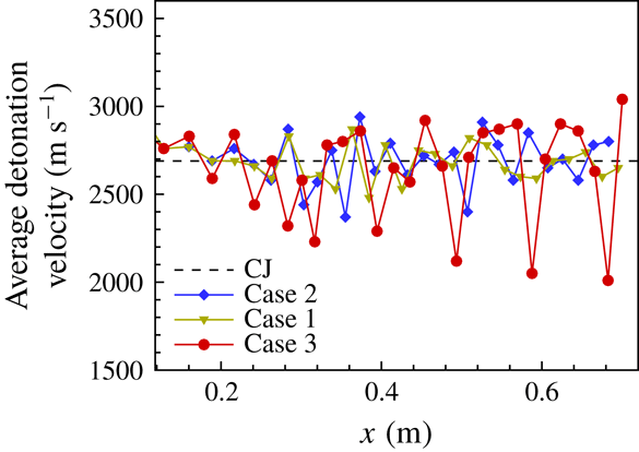
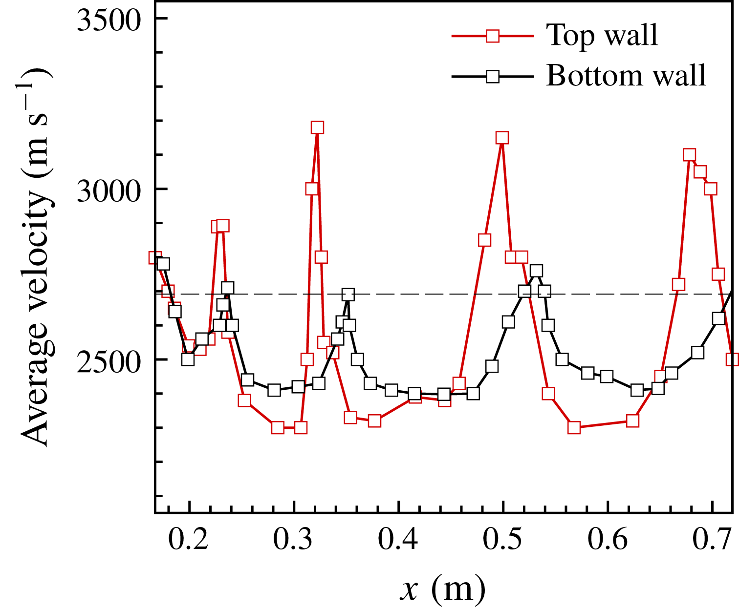
, which is comparable with that of the numerical studies by Calhoon & Sinha (Reference Calhoon and Sinha2005) and Kessler et al. (Reference Kessler, Gamezo and Oran2012). Furthermore, figure 18 shows the instantaneous detonation velocity as a function of distance for these three cases. For Case 1, the velocity oscillates around the CJ value, with small amplitude. However, the oscillation amplitude increases as the concentration gradient steepens. For Case 3, the oscillations along the top and bottom walls are obviously different, as shown in figure 19; comparison of the velocities shows that the amplitude of velocity oscillation along the upper boundary is larger, while the average velocity along the bottom is lower. Hence, the front is inclined obviously. On average the velocity exhibits large-amplitude fluctuations for single-head propagation and the portion below the CJ value is more substantial, hence having a lower average velocity. As such, we present next an explanation of the velocity deficit.
Average detonation velocity versus concentration gradient.

Instant detonation velocities as a function of distance.

Instant detonation velocities along the top and bottom walls as a function of distance for Case 3.

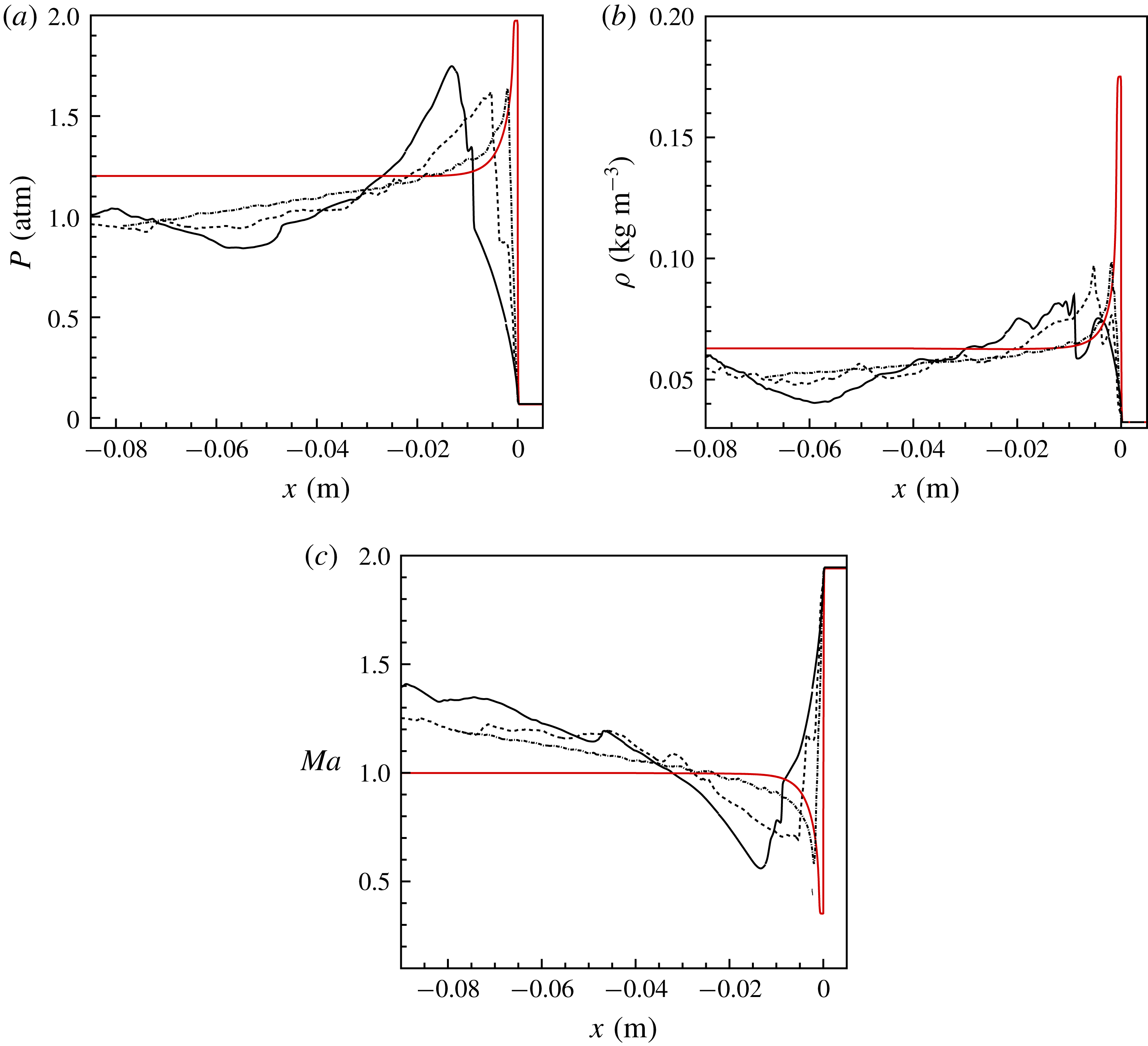
Averaged pressure (a), density (b) and Mach number (c): dotted line, Case 1; dashed line, Case 2; solid line, Case 3. Negative value in
 $x$
-coordinate denotes the downstream distance from the front.

The above discussion shows that as the concentration gradient steepens, the inclination of the detonation front increases and the global detonation structure is elongated. The amount of unreacted
 $\text{H}_{2}$
and species downstream increases and as such reaction equilibrium is reached more slowly. To demonstrate this, the average reaction zone structure for Cases 1–3 was determined in the range of
 $0.5~\text{m}\leqslant x\leqslant 0.72$
m. Edwards, Jones & Phillips (Reference Edwards, Jones and Phillips1976) found experimentally that sonic surfaces were delayed with respect to the surface where the chemical reaction was deposited in the flow. Therefore, a hydrodynamic thickness containing all unbalance was used by Radulescu et al. (Reference Radulescu, Sharpe, Law and Lee2007) to explain the elongated structure with delayed reaction and flow equilibrium. Radulescu et al. (Reference Radulescu, Sharpe, Law and Lee2007) made a significant study comparing a statistically averaged detonation structure with the steady solution for a single-head detonation propagating in a uniform mixture. They studied the average structure of a single-head detonation through the Favre-averaged detonation profiles in time and space in the frame of reference moving with the average detonation velocity. For highly unstable detonation, they showed that the average detonation structure is a meaningful concept that allows rationalization of the detonation wave velocity, the global rate of energy release inside the structure and the location of the sonic surface. Consequently, we also provide the Favre-averaged reaction zone profiles for pressure, density and Mach number (in the coordinate system moving with the average speed of the detonation), shown in figure 20 along with the ideal ZND solution; the flow Mach number in the detonation frame was obtained by assuming the mean sound speed, as in Radulescu et al. (Reference Radulescu, Sharpe, Law and Lee2007). Indeed, we observe from figure 20 that in the non-homogeneous mixture the average detonation structure thickens, as compared with that of the one-dimensional steady structure for a stoichiometric mixture, and steepening concentration gradient thickens the average reaction zone structure. This compares qualitatively with the hydrodynamic thickness in the highly unstable detonation of Radulescu et al. (Reference Radulescu, Sharpe, Law and Lee2007). However, for Case 1, the mean sonic plane can be observed clearly, while it is delayed as the concentration gradient steepens. This is caused by the flow fluctuation caused by the strongly local non-equilibrium reaction produced by the unreacted
 $\text{H}_{2}$
downstream, as seen in figures 8, 10 and 12. By approximating the first point where the Mach number is closest to unity as the mean sonic plane in the downstream flow, the respective values are:
 ${\sim}0.025$
m for Case 1, 0.035 m for Case 2 and 0.05 m for Case 3; see figure 20(c). This demonstrates that shock compression in a detonation initiates chemical reactions through the high-temperature and high-pressure environment it creates. The average structure departs significantly from the ideal structure. This non-equilibrium is extended far downstream as the concentration gradient steepens. Consequently, reaction equilibrium cannot reach the mean sonic point. For Case 3, transverse shock waves propagate through these thick layers of unburned material, further compressing and heating the mixture, which hastens reaction. The layer of unreacted material is thick enough and the transverse shock is strong enough to initiate a detonation that propagates through this layer normal to the direction of the leading detonation, namely the transverse detonation shown in figure 15. Due to the existence of the transverse detonation, the average path takes on an obvious second compression effect.
For Case 3, the single-head mode differs from the other cases in which sustaining is by the collision of triple points. The presence of the transverse detonation is due to the extended frontal structure led by the increased concentration gradient, which leads to the formation of a wider band of the gas compressed by the leading shock. Due to interaction of the leading shock with the gradient, the mixture globally is homogenized, while the
 $\text{H}_{2}$
concentration is increased locally, leading to more unreacted matter. As the transverse detonation runs from the lean layer to the richer layer in the compressed zone, the residue
 $\text{O}_{2}$
in the fuel-lean layer behind the front is convected into the fuel-rich layer, enhancing mixing of the unreacted matter downstream. However, the delayed reaction of much unreacted
 $\text{H}_{2}$
led by the steepened concentration gradient delays substantially the reaction equilibrium, relative to the average sonic point. Fluctuation of the species mass fraction behind the front is stronger than that in the other two cases and decays as it becomes far away from the front, showing that hydrodynamics and reaction kinetics do not reach equilibrium.
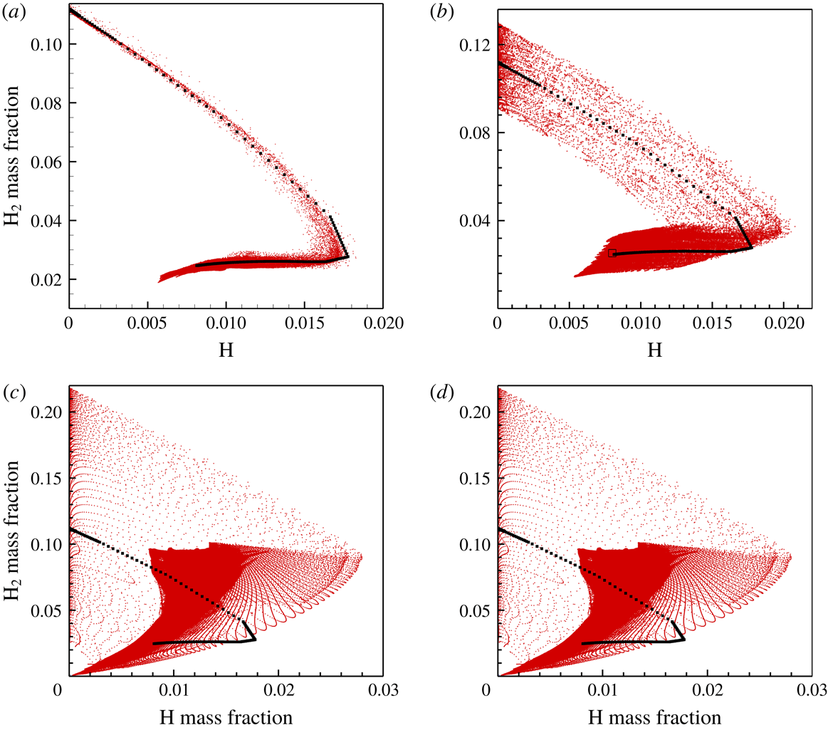
This single-head detonation differs from that in uniform media. A main track produced by strong transverse detonation is followed by a minor track led by weak triple point. To further identify the extent of non-equilibrium at the sonic plane, scatter plots of
 $\text{H}_{2}$
and H mass fraction in grid points are obtained and compared with the theoretical solution, as shown in figure 21. The squares in figure 21 indicate that
 $\text{H}_{2}$
and H mass fractions are, respectively, 0.03 and 0.0081 at the ideal sonic plane. However, the majority of scatterers of unreacted
 $\text{H}_{2}$
are above the constant of 0.03, indicating that the downstream
 $\text{H}_{2}$
is still active and reacts steadily. Furthermore, the gas state at the upper boundary of the scatterers goes beyond the range of the ideal CJ plane, substantiating that complete equilibrium is delayed considerably behind the ideal CJ state (sonic plane). As the concentration gradient increases, reaction equilibrium takes longer to reach. Consequently, this identifies that the non-equilibrium reaction leads to a delay of the sonic plane and even the absence of a mean sonic point.
Scatter plots of
 $\text{H}_{2}$
and H mass fraction with homogeneous mixture (a) and concentration gradient (b–d) in grid points. Black squares denote the steady solution.

In summary, a steepening concentration gradient promotes detonation cellular instability and leads to more unreacted
 $\text{H}_{2}$
downstream. As a result, due to non-equilibrium chemical reaction, attainment of the mean sonic point is significantly delayed. The non-equilibrium is extended further downstream and hence aggravates the deficit of detonation velocity as the concentration gradient steepens.
4.4 Justification of detonations with and without viscosity diffusion
We next note that Romick, Aslam & Powers (Reference Romick, Aslam and Powers2015) found through the calculation of one-dimensional viscous detonations with supporting piston and detailed
 $\text{H}_{2}$
–air mechanism that, for moderate unstable detonation, the effect of viscosity is weakened such that the results obtained by the Navier–Stokes equations are indistinguishable from the inviscid predications as the overdriven degree decreases. Oran et al. (Reference Oran, Weber, Stefaniw, Lefebvre and Anderson1998) performed a series of Navier–Stokes computations with detailed chemical kinetics and observed similar detonation structure for both Euler and Navier–Stokes equations. Based on their observation, they suggested that the small-scale structures that are eliminated in Euler computations do not affect the overall features of the detonation structure nor the reactive dynamics in the detonation structure. Radulescu et al. (Reference Radulescu, Sharpe, Law and Lee2007) suggested that in irregular structure detonation, turbulence mixing causes the consumption of most portions of the gases that cannot be ignited by shock compression, as suggested earlier by Subbotin (Reference Subbotin1975) and Gamezo et al. (Reference Gamezo, Desbordes and Oran1999). Small-scale vortices at the boundaries of the unreacted pockets produced by R–M and K–H instabilities (Radulescu et al.
Reference Radulescu, Sharpe, Law and Lee2007) promote the turbulent mixing of burnt and unburnt gases. Therefore, with the appearance of these features, local diffusion plays a noticeable role in the burning of the unreacted pockets by convective transport. Maxwell et al. (Reference Maxwell, Bhattacharjee, Lau-Chapdelaine, Falle, Sharpe and Radulescu2017) indicated through large-eddy simulation of multi-dimensional detonation in channels that the burning rate of unreacted pockets from their boundaries through surface turbulent flames is approximately 3–7 times larger than that of the laminar ones at the local conditions. Subsequently, the effect of diffusion on detonation behaviour is discussed when explicit physical diffusion is introduced as the cutoff length scale below which physical diffusion properly works.
Histories of shock pressure for Case 3: (a)
 $\unicode[STIX]{x1D6FF}x=2\times 10^{-5}$
m, (b)
 $\unicode[STIX]{x1D6FF}x=1\times 10^{-5}$
m.

For Cases 1 and 2, there is an obvious unreacted pocket behind the front in the fuel-rich region. It is of interest to see how the burning of the unreacted pockets is affected by changing the numerical diffusion. We selected Case 2 to conduct the simulation with
 $\unicode[STIX]{x1D6FF}x=2\times 10^{-5}$
m for the assessment of the role of numerical diffusion in the burning of the unreacted pockets. It can be seen from figure 22 that at
 $t=217.89~\unicode[STIX]{x03BC}\text{s}$
, the global frontal structure is consistent with that obtained with
 $\unicode[STIX]{x1D6FF}x=1\times 10^{-5}$
m, while finer structure is observed for the higher resolution. For
 $\unicode[STIX]{x1D6FF}x=2\times 10^{-5}$
m, an unreacted pocket can be observed in the fuel-rich region, its dimension being
 ${\sim}1\times 10^{-3}$
m. For
 $\unicode[STIX]{x1D6FF}x=1\times 10^{-5}$
m, the unreacted pocket still forms behind the inclined front in the fuel-rich layer, with a dimension of
 ${\sim}2\times 10^{-3}$
m and as such is larger than that for
 $\unicode[STIX]{x1D6FF}x=2\times 10^{-5}$
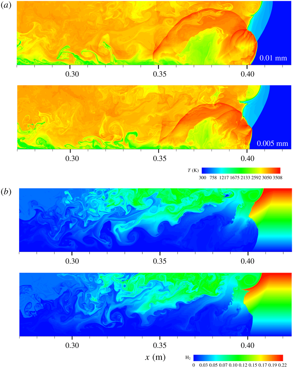
m because of the smaller numerical diffusion. By comparing results with these two levels of grid resolution, it is found that burning the unreacted pocket becomes difficult due to the lack of physical diffusion as the grid resolution increases and thus numerical diffusion reduces. Consequently, the lower resolution enhances the burning rate of the unreacted pocket, leading to the observed enhancement of the consumption of the pocket. In non-uniform detonation, diffusion modifies the inhomogeneity of the mixture besides the enhancement of turbulence mixing. Hence, consideration of physical diffusion could be especially relevant for non-homogeneous mixture, although the Euler model describes the main characteristics of the detonations in the concentration gradient. However, unreacted matter in non-homogeneous media is easier to be produced by the concentration gradient. Burning the unreacted matter is more related to turbulence diffusion. Consequently, we have conducted calculations of viscous and inviscid detonations in the mixture with the transversal concentration gradient by solving the Navier–Stokes and Euler equations.
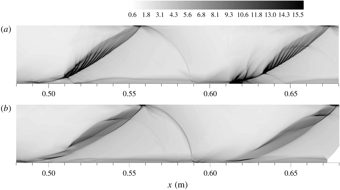
Histories of shock pressure for Case 2: (a) Euler, (b) Navier–Stokes.

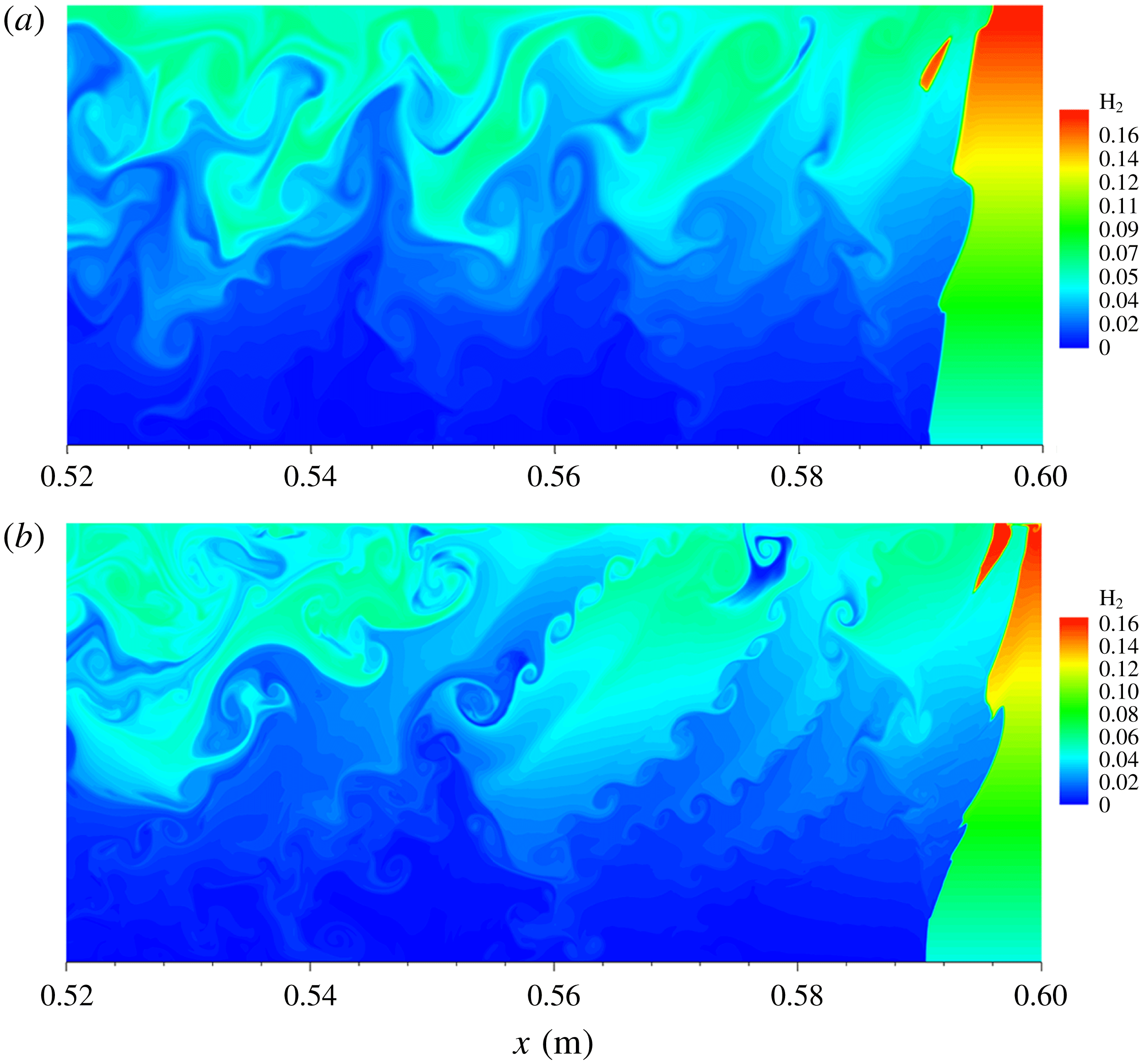
Detonation structures with and without diffusion for Case 3. (a) Temperature and (b)
 $\text{H}_{2}$
mass fraction contours.

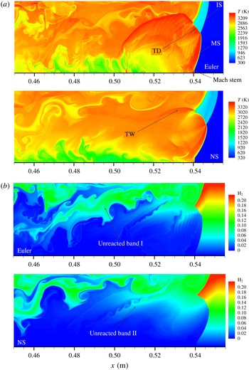
Figure 23 shows the detonation cell structure obtained with Euler and Navier–Stokes equations for Case 3. It is seen that for the viscous and inviscid cases, the global cell characteristics are qualitatively similar, with minor differences of the finer structure, demonstrating that the Euler model is able to describe the main feature of the detonation with the concentration gradient in Case 3. This also indicates that the present results are valid for examining the global feature of the cellular detonation in the non-homogeneous mixture. However, if the finer structure of the detonation is required to be studied, as the numerical resolution is enhanced and numerical diffusion is reduced, the description of the detonation with the transversal concentration gradient favours the viscous diffusion model. Figure 24 shows typical temperature and
 $\text{H}_{2}$
mass fraction contours in the frontal structures for the cases with and without diffusion. It is seen that the frontal structures globally are similar for these two cases, consisting of Mach shock, incident shock, transverse wave and Mach stem near the bottom. The transverse detonation is observed and a long transverse wave extends downstream in both viscous and inviscid simulations. Nevertheless, in the inviscid case the transverse wave is stronger so that transport of the
 $\text{O}_{2}$
in the fuel-lean layer into the fuel-rich layer is stronger. Consequently, the unreacted band I is consumed more substantially, compared with that in the viscous case. Although small-scale vortices at the boundary of the unreacted band I, caused by R–M instability, are observed obviously and play a role in the burning rate of the remaining
 $\text{H}_{2}$
and
 $\text{O}_{2}$
downstream, consumption of the unreacted band I is mainly caused by the role of the transverse wave. Furthermore, fine structures appear at the front of the transverse detonation for the Euler case, while they are suppressed in the Navier–Stokes case, as shown in figure 24(a). The unreacted band I is thinner for the viscous case than for the inviscid case, demonstrating that the burning rate of the unreacted matter is enhanced by adding the viscous diffusion term. This is reasonable as with decreasing numerical resolution, physical diffusion serves explicitly to influence the burning rate of unreacted matter. However, qualitative agreement still is observed between the structures obtained by solving the Euler and Navier–Stokes equations.
4.5 Effect of channel width on detonation mode with transversal concentration gradient
Before the detonation encounters the concentration gradient, there are only a few cells across the channel (4–5). Since the concentration gradient acts to increase the cell size and decrease the quantity of cells (e.g. figure 5), there is a likelihood that some of the results may be due to mode-locking based on the width of the (rigid-wall) channel. We carried out the simulation of the detonation for a constant concentration along the entire channel of 0.036 m to examine the long-time behaviour, and found that the cell pattern does not flip to larger size, as shown in figure 25. This demonstrates that the present cell should be intrinsic. Generally, the mode-locking phenomenon is observed in the situation where the channel width is not large enough to accommodate one cell size. For the uniform mixture, it is easy to argue that mode-locking influences the cell pattern through increasing the channel width. The detonation behaviour in a channel width of
 $d=0.072$
m for Case 2 is simulated to investigate the effect of rigid wall on the detonation cell and to explain the mode-locking based on the channel width. It is seen that in the region of
 $x=0$
–0.02 m, the cell regularity agrees globally with that in the case of 0.036 m (figure 25), showing that the mode-locking effect is weak for detonation in a uniform mixture. However, in the non-homogeneous region the detonation cell depends significantly on the channel width. In the wider channel, by fixing the gradient in Case 2, increasing the channel width allows a wider range of equivalence ratios, from
 $\unicode[STIX]{x1D719}=0$
at the bottom to
 $\unicode[STIX]{x1D719}=2$
at the top boundary. Consequently, the detonation mode in the wider channel differs significantly from that in the 0.036 m channel; see figure 26. The detonation is weaker since triple points weaken as they move into the richer and leaner regions. As a result, the reflection waves are not strong and there is no generation of new triple points, leading to a reduction of the number of triple points and an increase of the cell size as compared with the narrow channel.
Detonation cell in uniform mixture:
 $\unicode[STIX]{x1D719}=1$
,
 $p_{0}=0.067$
atm,
 $T_{0}=300$
.

Detonation cell in the wider channel of 0.072 m for Case 2.

Detonation cell in the wider channel of 0.072 m for Case 2: (a)
 $t=200.6$
, (b) 206.6, (c) 211.8, (d) 216.7 and (e)
 $222.0~\unicode[STIX]{x03BC}\text{s}$
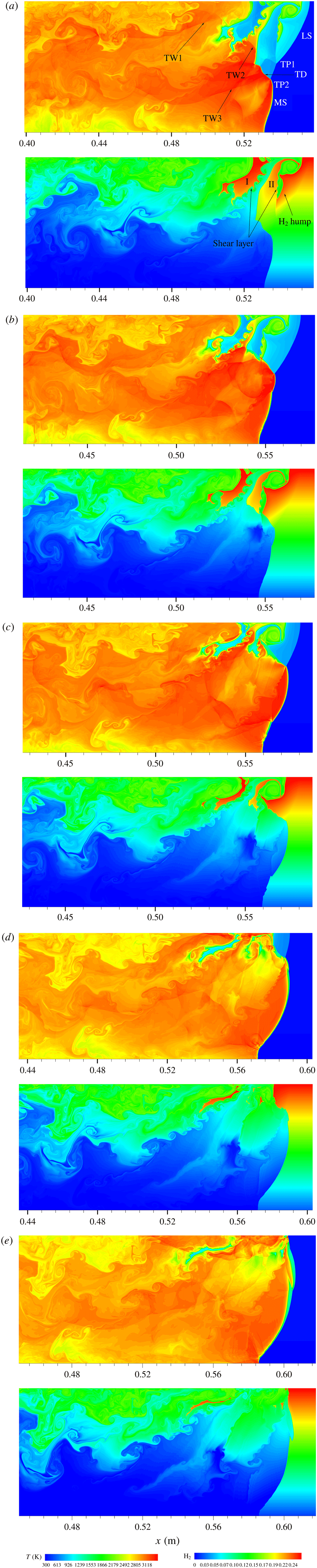
. Leading shock, LS; transverse detonation, TD; Mach shock, MS; transverse wave 1, 2, 3, TW1, TW2, TW3.

Figure 27 shows the detonation structure at different times to reveal the interaction of the transverse wave and the burning of the unreacted pockets in more detail. It is seen that at
 $t=200.6~\unicode[STIX]{x03BC}\text{s}$
, the front consists of leading shock, transverse detonation, transverse shock, Mach shock and the Mach stem. A secondary triple point (TP1) moves downwards and a main triple point (TP2) runs upwards, associated with a transverse detonation. Note that the leading shock decouples from the reaction zone and a thick compressed zone forms in the fuel-rich layer, in which the shocked gas is burnt partially while the rest is not consumed. As a result, two blocks of unreacted pockets form behind the leading shock front, with dimensions of
 ${\sim}0.010$
m for pocket I and
 ${\sim}8\times 10^{-3}$
m for pocket II. Some small-scale vortices are produced by R–M and K–H instabilities at the boundary of the pocket. Also large vortical structure near the upper boundary is formed following the leading shock, and the shocked gas reacts earlier in the large vortical structure and at the slipping shear surface induced by the secondary triple point. Downstream near the upper boundary, TW1 moves downwards, while TW2 associated with the main triple point runs upwards. The leading shock convects the
 $\text{H}_{2}$
fuel into the region of lower fuel concentration and consequently a large area of
 $\text{H}_{2}$
hump is formed, as shown in figure 27(a). At
 $t=206.6~\unicode[STIX]{x03BC}\text{s}$
, a new Mach shock is produced after TP2 collides with TP1; and the resulting triple point runs downwards, while TP2 continues moving towards the upper wall. Meanwhile the transverse detonation and the burning at the slip shear layer lead to substantial consumption of pocket I. As TW2 interacts with pocket II, promotion of the burning rate means it is consumed rapidly so that the size of pocket II reduces significantly and the fine structure at the boundary also is almost burnt out. At
 $t=211.8~\unicode[STIX]{x03BC}\text{s}$
, TW2 interacts with pocket I, leading to it moving upwards and globally becoming parallel to the wall. The interaction of TW2 enhances significantly the mixing and burning rate of pockets I and II. The size is further reduced to
 ${\sim}2.5\times 10^{-3}$
m for pocket I and
 ${\sim}2\times 10^{-3}$
m for pocket II. At
 $t=216.7~\unicode[STIX]{x03BC}\text{s}$
, TW2 collides with the upper wall and the reflected wave interacts with pocket II; meanwhile TW2 interacts with pocket I, leading to its rapid consumption, as shown in figure 27(d). At
 $t=222.0~\unicode[STIX]{x03BC}\text{s}$
, the reflected TW2 interacts with pocket II again and causes it to become horizontal; it is left far downstream, with a dimension of
 ${\sim}1\times 10^{-3}$
m.
In summary, in the uniform region the detonation cell does not change significantly with an increase of the channel width. However, the detonation mode in the mixture with the transversal concentration gradient depends strongly on the channel width and the confinement. This is because a wider channel is likely to allow a correspondingly wider range of the equivalence of the
 $\text{H}_{2}{-}\text{O}_{2}$
mixture. Hence, the leaner and richer mixtures near the upper and lower boundaries always render the shocks weaker so that the role of the reflection wave is weak, which effectively weakens the confinement. As a result, the detonation behaviour is considerably different from that in the narrow channel. It is found that in the wider channel, an unreacted pocket is easier to form and its dimension is much larger than that in the narrow channel. For Case 3, in the channel of 0.036 m the equivalence is equal to 2 at the upper boundary, but there is no observed unreacted pocket in the fuel-rich layer due to the coupling role of strong transverse detonation and confinement.
5 Conclusions and discussion
High-resolution simulations were conducted to study the detonation behaviour in a transversal concentration gradient. It is found that for a small concentration gradient, detonation is sustained with multi-head mode, resembling the detonation characteristics in a homogeneous mixture. However, steepening the concentration gradient promotes detonation instability. For a sufficiently large gradient, the single-head mode similar to detonation in mixtures with high activation energy (Gaathaug, Vaagsaether & Bjerketvedt Reference Gaathaug, Vaagsaether and Bjerketvedt2014) is observed. While the concentration gradient renders significant enhancement of the local strength of the shock wave affected by strong local explosion, it reduces the average detonation velocity as compared with that in a uniform mixture. The deficit of the average detonation velocity is attributed to the increase in the dimension of the average detonation structure (hydrodynamic thickness) due to non-equilibrium reaction extending downstream. Steepening the concentration gradient enhances globally the cellular instability of detonation and leads to more unreacted
 $\text{H}_{2}$
downstream. As a result, due to non-equilibrium chemical reaction, attainment of the mean sonic point is significantly delayed and even cannot be clearly identified. The state of non-equilibrium is extended further downstream and hence increases the deficit of the detonation velocity.
The importance of using a mean steady detonation profile to determine the location of the effective sonic plane was highlighted by Radulescu et al. (Reference Radulescu, Sharpe, Law and Lee2007). One-dimensional analysis of a two-dimensional, moderately unstable detonation wave was explored computationally by Radulescu et al. (Reference Radulescu, Sharpe, Law and Lee2007) through spatial and time averaging of the unsteady structure, showing that an average detonation structure is meaningful and allows rationalization of the detonation velocity, global rate of energy release inside the structure and location of the sonic surface. It was found that the interplay between the chemical reaction and hydrodynamic fluctuations leads to the average dimension being extended in two-dimensional detonation structure. The mean sonic surface in cellular detonation with the transverse gradient is valid for study of the average detonation structure by comparing with steady detonation, as discussed in appendix B. The averaged structure of detonation is just one of the methods to estimate hydrodynamic thickness, in which due to the transversal gradient, reaction equilibrium is delayed significantly, compared with the mean sonic surface. Thus, the investigation of hydrodynamic thickness in the averaged one-dimensional structure of cellular detonation is a fruitful approach in the development of detonation theory.
Radulescu et al. (Reference Radulescu, Sharpe, Law and Lee2007) first revealed experimentally and numerically that in the extended detonation structure on average, the potential role of viscosity and diffusion needs to be considered. They found that the flow and reaction fluctuations extended the dimension of the detonation structure on average for mildly unstable detonation in a uniform mixture. However, as spatial discretization of the energy source is introduced, the classic CJ solution breaks down. Radulescu et al. (Reference Radulescu, Sharpe, Law and Lee2007) identified the energy into flow fluctuation downstream and its further dissipation, and verified the experimental findings of Edwards et al. (Reference Edwards, Jones and Phillips1976) on the delayed sonic surface with respect to the surface where the chemical reaction was deposited in the flow. Mi et al. (Reference Mi, Timofeev and Higgins2017) found that the flow is not in equilibrium at the effective sonic surface for the cellular detonation in media with spatial discretization of energy and the average detonation velocity is higher than the CJ value for constant total heat release, verifying that the classic CJ criterion assuming a homogeneous medium based on averaged properties is not always applicable to predict the detonation velocity in a spatially inhomogeneous system. However, for the present inhomogeneous media with realistic chemical mechanism, the flow and reaction equilibria are far from being reached at the location of the sonic surface due to reaction fluctuations produced by the non-equilibrium local reaction of the unreacted matter downstream. Both the chemical reaction and flow do not reach equilibrium due to the coupling of the flow fluctuations and reactions resulting from the unreacted matter at the effective sonic plane. Equilibrium becomes difficult to be reached due to the increased amount of unreacted matter behind the front as the concentration gradient steepens, as indicated by stronger fluctuations of species mass fractions in figure 12. Consequently, deficit of the average detonation velocity is observed in mixtures with concentration gradient, which is similar to the calculations in which the average velocity is lower than that in a uniform mixture. In the widened structure, burning unreacted matter has an important influence on the cellular dynamics and further on the detonation velocity; while the mixing and burning rates of the unreacted matter are related closely to the R–M and K–H instabilities. This favours vorticity production and much of the turbulent fluctuation is expected to be driven directly by the chemical energy via violent volumetric expansion of the gas inducing pressure waves at small-scale turbulence, which was introduced by numerical viscosity in the present simulations. Explicit physical diffusion needs to be introduced as a cut-off length scale below which physical viscosity properly serves to influence the burning rate of unreacted matter. A correct model for the global energy release in highly unstable detonations should involve the mechanism of turbulent mixing between gases at various stages of their diffusionless oxidation process, generated by K–H and R–M instabilities. Hence, the turbulence combustion model to predict the energy deposited in the downstream fluctuations for non-ideal detonation merits study in future work.
Acknowledgements
This research was supported by the National Key R&D Program of China (no. 2017YFC0804700), National Natural Science Foundation of China under grant 11732003, Science Challenge Project (TZ2016001) and Beijing Natural Science Foundation (8182050).
Appendix A. Verification of relative grid resolution
Histories of shock pressure for Case 3: (a)
 $\unicode[STIX]{x1D6FF}x=2\times 10^{-5}$
m, (b)
 $\unicode[STIX]{x1D6FF}x=1\times 10^{-5}$
m, (c)
 $\unicode[STIX]{x1D6FF}x=5\times 10^{-6}$
m.

Histories of shock pressure along the middle line of the channel for Case 3 (
 $t=202.25~\unicode[STIX]{x03BC}\text{s}$
).

The single-head detonation in figure 5 is resolved by refining the mesh to
 $\unicode[STIX]{x1D6FF}x=5\times 10^{-6}$
m. Figure 28 shows the maximum pressure histories for the grid resolution of
 $\unicode[STIX]{x1D6FF}x=1\times 10^{-5}$
and
 $5\times 10^{-6}$
m. It can be seen that with mesh refining, the global features of the detonation tend to be consistent, with minor differences in the fine structures. Comparison of the shock pressure along the middle line of the channel indicates quantitatively that the results with
 $\unicode[STIX]{x1D6FF}x=1\times 10^{-5}$
m are valid; see figure 29. Figure 30 shows almost consistent characteristics of the temperature and
 $\text{H}_{2}$
mass fraction contours at
 $t=148.2~\unicode[STIX]{x03BC}\text{s}$
for the single-head detonations with
 $\unicode[STIX]{x1D6FF}x=1\times 10^{-5}$
and
 $5\times 10^{-6}$
m. Consequently, the gird resolution of
 $\unicode[STIX]{x1D6FF}x=1\times 10^{-5}$
m is sufficient to capture the main feature of the single-head detonation with the steeper gradient. Also the
 $\text{H}_{2}$
hump for
 $\unicode[STIX]{x1D6FF}x=5\times 10^{-6}$
m is similar to that for
 $\unicode[STIX]{x1D6FF}x=1\times 10^{-5}$
m. We observe that unreacted band with
 $\unicode[STIX]{x1D6FF}x=5\times 10^{-6}$
m is wider than that with
 $\unicode[STIX]{x1D6FF}x=1\times 10^{-5}$
m. This is reasonable because for the lower grid resolution the large numerical diffusion can lead to the enhancement of burning rate of the unreacted
 $\text{H}_{2}$
left downstream. Nevertheless, for
 $\unicode[STIX]{x1D6FF}x=1\times 10^{-5}$
m, more small-scale structures appear at the boundary of the unreacted band.
Detonation front structure for Case 3 (
 $t=202.25~\unicode[STIX]{x03BC}\text{s}$
). (a) Temperature and (b)
 $\text{H}_{2}$
mass fraction contours.

We next present a further assessment of the time-step convergence for the highly unstable detonation in Case 3, which requires higher grid resolution. Two mesh sizes of
 $\unicode[STIX]{x1D6FF}x=2\times 10^{-5}$
and
 $1\times 10^{-5}$
m were used to simulate Case 3. Figure 31 shows that for
 $\unicode[STIX]{x1D6FF}x=2\times 10^{-5}$
m, detonation takes single-head mode and the main track can be captured, with irregular cell structure. For
 $\unicode[STIX]{x1D6FF}x=0.01$
, while the single-head mode still is present, with increasing grid solution the finer structure appears in the track of the cell. However, the main cell characteristics do not vary significantly. Consequently, the results obtained with the grid resolution of
 $\unicode[STIX]{x1D6FF}x=1\times 10^{-5}$
m are valid. The present grid convergence is obtained for the Euler equations with a non-diffusive formulation. Because of the absence of physical diffusion, when the grid size is refined further, the finer features are seen. Hence, the resolution of
 $\unicode[STIX]{x1D6FF}x=1\times 10^{-5}$
m is enough to study the effect of the concentration gradient on the propagation characteristics and to reveal the main cell structures. Furthermore, we have reduced the CFL number by half of the original value to carry out the simulation of Case 3 with
 $\unicode[STIX]{x1D6FF}x=1\times 10^{-5}$
m. We observe from figure 31(b,c) that as the time step decreases, the main tracks do not change, indicating that the present time step is enough for numerical resolution.
Histories of shock pressure: (a)
 $\unicode[STIX]{x1D6FF}x=2\times 10^{-5}$
m and
 $\text{CFL}=0.2$
, (b)
 $\unicode[STIX]{x1D6FF}x=1\times 10^{-5}$
m and
 $\text{CFL}=0.2$
, (c)
 $\unicode[STIX]{x1D6FF}x=1\times 10^{-5}$
m and
 $\text{CFL}=0.1$
.

In summary, due to the existence of the concentration inhomogeneity, numerical diffusion always influences the concentration gradient in detonation structure and thus leads to detonation behaviour sensitive to the grid resolution for the inviscid case. Although the Euler model can describe the main behaviour of the detonation with the gradient substantiated by the above results, it is likely that a description of detonation propagating in the mixture with a transversal concentration gradient favours the use of the Navier–Stokes model for more physical results.
Appendix B. Justification of a mean sonic surface for unstable cellular detonation
A sonic locus has physical meaning for one- or two-dimensional steady flows in the frame of a steadily travelling shock. Non-equilibrium fluctuations from downstream supersonic flow are closed by the sonic surface so that they cannot propagate upstream to influence the leading shock. However, for one-dimensional unsteady detonation, there is a separatrix of the flow behind the front such that the characteristics upstream of it can eventually reach the leading shock, while those downstream cannot reach the leading shock (Kasimov & Stewart Reference Kasimov and Stewart2004). Although a real detonation structure is non-steady and three-dimensional, the averaged velocity is found to agree with steady one-dimensional CJ theory, even for near-limit spinning detonations. A hydrodynamic thickness is determined by energy release dynamics in the region between the detonation shock and sonic locus, where flow and reaction reach equilibrium. The thickness based on sonic conditions of the averaged properties is calculated through an alternative approach attempted by Radulescu et al. (Reference Radulescu, Sharpe, Law and Lee2007) by averaging the field data obtained in a numerical simulation of two-dimensional cellular detonations. For cellular detonation in a uniform mixture, this is reasonable because globally equilibrium processes behind the detonation front are achieved approximately at the same surface. For cellular detonations in an inhomogeneous mixture, it is also supported by the identification of an effective sonic surface in figure 32, which shows the separatrix of
 $Ma=1$
to divide globally supersonic and subsonic flows. Mach number (in the shock-attached frame) first is calculated for the whole flow field and then the lines where the Mach number equals unity are figured out. It is seen that while the equilibrium of reaction in downstream flow is delayed significantly in the rich layer, the flow region between the mean sonic surface and shock can still reflect global detonation structure. Consequently, the mean sonic surface in cellular detonation has physical meaning for study of average detonation structure by comparing with steady detonation.
Characteristics of flow behind the front for viscous detonation in figure 24: black lines are for
 $Ma=1$
, which is calculated in the frame of travelling shock;
 $\unicode[STIX]{x1D712}$
is thermicity.

Appendix C. Track of triple point at transversal concentration gradient
Instant detonation velocities as a function of distance: (a) pressure, (b) OH mass fraction, (c) temperature, (d) histories of shock pressure in figure 5(c).

We chose Case 3 to further examine the effect of transversal concentration gradient on the triple-point track and compared it with that in uniform media. It is seen that half of the detonation cell spans the entire channel, as shown in figure 5. Hence, evolution of the detonation front in one detonation cell is zoomed and the corresponding instantaneous frontal structures are shown in figure 33. It is seen that at
 $t=215.2~\unicode[STIX]{x03BC}\text{s}$
, the detonation front is substantially inclined, with one triple point running along the highly inclined front and a transverse shock behind it. Globally, the leading shock is coupled with the reaction layer. Meanwhile, a short Mach stem stands near the bottom to meet the boundary condition. Nevertheless, here the OH mass fraction is very low, indicating that chemical reaction behind the Mach stem does not occur due to the extremely lean fuel; see figure 33(b). With the incident shock decaying, the induction zone thickens and the leading shock decouples with reaction at
 $t=222.3~\unicode[STIX]{x03BC}\text{s}$
, shown in figure 33(c). The inclined leading shock can bring the fuel in the middle into the fuel-lean layer near the bottom. At some time, the triple point collides with the lower wall, leading to local explosion near the lower wall where the mixture is homogenized by the transverse shock. Hence, high OH mass fraction is observed here, shown in figure 33(b). The local explosion advances and evolves into a leading detonation, which then develops into a transverse detonation at
 $t=225.4~\unicode[STIX]{x03BC}\text{s}$
, and propagates into the region with chemical stoichiometry with fine structure present on its front at
 $t=228.1~\unicode[STIX]{x03BC}\text{s}$
. As the incident shock decays, the induction zone near the top thickens, in which the shocked gas is far away from stoichiometry (
 $\unicode[STIX]{x1D719}\sim 2.0$
). When the transverse detonation moves into this zone, it weakens and slows down at
 $t=231.2~\unicode[STIX]{x03BC}\text{s}$
. This is also why the tracks are more curved as compared with those in the uniform mixture. Due to the existence of the strong transverse detonation, there is no bulk unreacted pocket behind the inclined front. Consequently, the average detonation velocity in Case 3 is not significantly lower than that in the other two cases. On the other hand, the leading detonation propagates forwards and catches up with the incident shock. At
 $t=234.1~\unicode[STIX]{x03BC}\text{s}$
, the inclination of the global detonation front weakens as the transverse detonation arrives at and collides with the upper wall, resulting in a reflected shock that moves downwards and starts a new cycle.