1 Introduction
In recent years, gel propellants have been widely used in rocket engine applications, with better performance than the traditional liquid propellants and solid propellants. A gel propellant is a time-dependent non-Newtonian fluid and usually has the properties of shear thinning (Yang & Zhang Reference Yang and Zhang2005). However, due to its high viscosity and rheological properties, it is difficult for a gel propellant to atomize, and its atomization mechanism has not been fully understood, which is the main bottleneck restricting the performance of gel rocket engines. Therefore, it is of great significance to study the fracture behaviour of non-Newtonian fluids.
Concerning researches on atomization mechanism of non-Newtonian fluids, most are based on viscoelastic fluids (Paul Reference Paul1968; Goldin et al. Reference Goldin, Yerushalmi, Pfeffer and Shinnar1969; Gordon, Yerushalmi & Shinnar Reference Gordon, Yerushalmi and Shinnar1973; Lee & Rubin Reference Lee and Rubin1975; Pearson Reference Pearson1976; Petrie & Denn Reference Petrie and Denn1976; Middleman Reference Middleman1977). In 1975, Crapper, Dombrowski & Jepson (Reference Crapper, Dombrowski and Jepson1975) studied surface wave growth on thin sheets of non-Newtonian fluids. In 1998, Liu, Brenn & Durst (Reference Liu, Brenn and Durst1998) succeeded in applying the method of analysing the instability of planar Newtonian sheets to that of planar non-Newtonian sheets. They investigated breakup instability for both symmetric and antisymmetric disturbances and effects of various parameters on the instability of viscoelastic fluids. It was found that viscoelasticity would make the sheets more unstable. Later, Kumar (Reference Kumar2001), Tomar et al. (Reference Tomar, Shankar, Shukla, Sharma and Biswas2006), Yang, Xu & Fu (Reference Yang, Xu and Fu2012) and Yang, Tong & Fu (Reference Yang, Tong and Fu2013) also conducted theoretical researches on the stability of non-Newtonian liquid sheets. Experimentally, Becerra & Carvalho (Reference Becerra and Carvalho2011) studied the effect of a high molecular weight polymer in the dilute regime on the critical flow rate that leads to curtain breakup. The rheological behaviour of the polymer solutions was characterized in both shear- and extension-dominated flow.
In engineering, when investigating the steady shear rheological behaviour of a gel propellant, the relationship between shear viscosity
 $\unicode[STIX]{x1D707}$
and shear rate
 $\dot{\unicode[STIX]{x1D6FE}}$
can be fitted as
 $\unicode[STIX]{x1D707}=k\dot{\unicode[STIX]{x1D6FE}}^{n-1}$
(Lee & Koo Reference Lee and Koo2010); therefore this kind of fluid is usually called a power-law fluid. Up to now, reports on the atomization mechanism of power-law fluids have been rare, most of which are focused on flow stability for power-law fluid films along an inclined plane. Lin & Hwang (Reference Lin and Hwang2000) used the method of normal mode to study linear stability for power-law liquid films flowing down an inclined plane. The results showed that shear-thinning liquid films along an inclined plane are more unstable than Newtonian ones, and the dimensional wave speed of shear-thinning liquids is faster than that of Newtonian ones. Balmforth, Craster & Toniolo (Reference Balmforth, Craster and Toniolo2003) found superposed layers of fluid flowing down an inclined plane are prone to disintegrate even in the limit of zero Reynolds number. They presented two versions of lubrication theory for superposed layers of a non-Newtonian fluid with power-law rheology and carried out both linear analysis and nonlinear numerical simulation. Amaouche, Djema & Abderrahmane (Reference Amaouche, Djema and Abderrahmane2012) conducted a linear stability analysis for a power-law fluid film flowing down an inclined plane with the method of lubrication theory and weighted residual approach. Also, they performed an incomplete regularization procedure to cure the rapid divergence of the reduced two-equation model. Jawadi, Boutyour & Cadou (Reference Jawadi, Boutyour and Cadou2013) proposed an asymptotic numerical method to solve the power-law flow problem. Comparisons with the numerical results found in the literature demonstrate the efficiency of the proposed numerical method. Ruyer-Quil, Chakraborty & Dandapat (Reference Ruyer-Quil, Chakraborty and Dandapat2012) studied the wavy regime of a power-law fluid flowing down an inclined plane under the influence of gravity, within the frame of the lubrication approximation and by means of the weighted residual approach. Considering the inadequacy of researches on stability of free power-law liquid jets or sheets, in this paper, a planar power-law liquid sheet with symmetric disturbances has been chosen to study its nonlinear stability. Both first-order dispersion equation and second-order interface disturbance are obtained. And the influence of power-law characteristics on sheet instability has also been studied.
2 Theoretical model
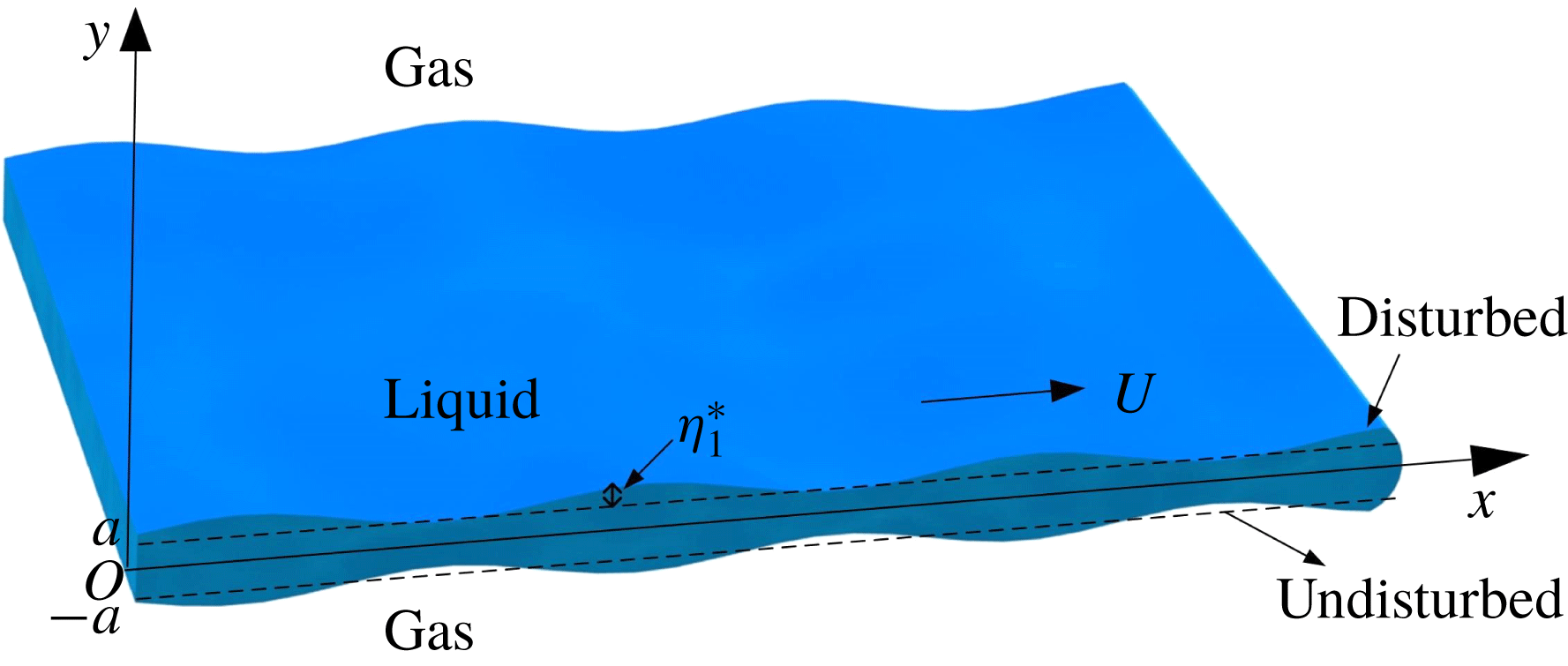
Imagine a uniform infinite free power-law liquid sheet surrounded by a stationary inviscid incompressible irrotational gas. For the liquid sheet, its density, thickness, coefficient of surface tension, power-law index and velocity are respectively denoted by
 $\unicode[STIX]{x1D70C}$
,
 $2a$
,
 $\unicode[STIX]{x1D70E}$
,
 $n$
(
 ${<}$
1) and
 $U$
. While for the gas,
 $\unicode[STIX]{x1D70C}_{g}$
and
 $p_{g}$
represent its density and pressure, respectively, as is shown in figure 1. Parameter
 $\unicode[STIX]{x1D702}_{j}^{\ast }$
indicates the disturbance amplitude of the upper or lower surface: when
 $j=1$
, it corresponds to the upper surface; when
 $j=2$
, it corresponds to the lower surface. Here, the influence of gravitational and magnetic fields is ignored.
Schematic diagram of free power-law sheets under symmetric disturbances.

2.1 Liquid phase
The governing equations for the liquid phase are
 $$\begin{eqnarray}\displaystyle & u_{x}+v_{y}=0, & \displaystyle\end{eqnarray}$$
 $$\begin{eqnarray}\displaystyle & \unicode[STIX]{x1D70C}(u_{t}+uu_{x}+vu_{y})=-p_{x}+\unicode[STIX]{x2202}_{x}\unicode[STIX]{x1D70F}_{xx}+\unicode[STIX]{x2202}_{y}\unicode[STIX]{x1D70F}_{xy}, & \displaystyle\end{eqnarray}$$
 $$\begin{eqnarray}\displaystyle & \unicode[STIX]{x1D70C}(v_{t}+uv_{x}+vv_{y})=-p_{y}+\unicode[STIX]{x2202}_{x}\unicode[STIX]{x1D70F}_{xy}+\unicode[STIX]{x2202}_{y}\unicode[STIX]{x1D70F}_{yy}, & \displaystyle\end{eqnarray}$$
where the liquid velocity field
 $\boldsymbol{u}=ui+vj$
and the stress tensor
 $\unicode[STIX]{x1D70F}_{ij}=\unicode[STIX]{x1D707}_{eff}(\dot{\unicode[STIX]{x1D6FE}})(\unicode[STIX]{x2202}_{i}u_{j}+\unicode[STIX]{x2202}_{j}u_{i})$
. The non-dimensional Carreau-law model is adopted as the constitutive model here, and
 $\unicode[STIX]{x1D707}_{eff}$
is an effective viscosity which is a function of the strain rate
 $\dot{\unicode[STIX]{x1D6FE}}$
:
 $$\begin{eqnarray}\unicode[STIX]{x1D707}_{eff}(\dot{\unicode[STIX]{x1D6FE}})=\left[1+\left(\frac{\dot{\unicode[STIX]{x1D6FE}}}{\dot{\unicode[STIX]{x1D6FE}}_{c}}\right)^{2}\right]^{(n-1)/2},\end{eqnarray}$$
where
 $\dot{\unicode[STIX]{x1D6FE}}_{c}$
denotes the critical shear rate of the power-law sheet, separating Newtonian and non-Newtonian behaviour of shear-thinning fluids (Ruyer-Quil et al.
Reference Ruyer-Quil, Chakraborty and Dandapat2012).
In the situation here, we assume that the sheet thickness is far smaller than the wavelength. Using the long-wave assumption, let the ratio of the sheet thickness and the wavelength satisfy
 $a/L=\unicode[STIX]{x1D716}\ll 1$
. With the selected characteristic wavelength
 $L$
, characteristic velocity
 $U$
and characteristic viscosity
 $\unicode[STIX]{x1D707}_{\ast }$
(
 $\unicode[STIX]{x1D707}_{\ast }=\unicode[STIX]{x1D707}_{n}(U/L)^{n-1}$
, where
 $\unicode[STIX]{x1D707}_{n}$
is the consistency coefficient), the dimensionless forms of the parameters are as follows:
 $y=a{\hat{y}}$
,
 $x=L\hat{x}$
,
 $\unicode[STIX]{x1D702}=a\hat{\unicode[STIX]{x1D702}}$
,
 $u=U\hat{u}$
,
 $v=\unicode[STIX]{x1D716}U\hat{v}$
,
 $t=(L/U)\hat{t}$
, liquid pressure
 $p=\unicode[STIX]{x1D707}_{\ast }(U/L)\hat{p}$
, stress tensor
 $\underset{=}{\unicode[STIX]{x1D749}}=\unicode[STIX]{x1D707}_{\ast }(U/L)\hat{\underset{=}{\unicode[STIX]{x1D70F}}}$
, shear rate
 $\dot{\unicode[STIX]{x1D6FE}}=(U/L)\hat{\dot{\unicode[STIX]{x1D6FE}}}$
, gas potential function
 $\unicode[STIX]{x1D6F7}=\unicode[STIX]{x1D716}UL\hat{\unicode[STIX]{x1D6F7}}$
, gas-to-liquid density ratio
 $\bar{\unicode[STIX]{x1D70C}}=\unicode[STIX]{x1D70C}_{g}/\unicode[STIX]{x1D70C}$
, Reynolds number
 $Re=\unicode[STIX]{x1D70C}U^{2-n}L^{n}/\unicode[STIX]{x1D707}_{n}$
, Weber number
 $We=\unicode[STIX]{x1D70C}U^{2}L/\unicode[STIX]{x1D70E}$
and gas pressure
 $P_{g}=Lp_{g}/\unicode[STIX]{x1D707}_{\ast }U$
. Here, the subscript
 $g$
denotes the corresponding parameters for the gas, while the hat represents the corresponding dimensionless form of each parameter.
Then the governing equations can be non-dimensionalized as follows (for the sake of convenience, the hat
 $\hat{\,}$
has been omitted):
 $$\begin{eqnarray}\displaystyle & \displaystyle u_{x}+v_{y}=0, & \displaystyle\end{eqnarray}$$
 $$\begin{eqnarray}\displaystyle & \displaystyle Re(u_{t}+uu_{x}+vu_{y})=-p_{x}+\unicode[STIX]{x2202}_{x}\unicode[STIX]{x1D70F}_{xx}+\frac{1}{\unicode[STIX]{x1D716}}\unicode[STIX]{x2202}_{y}\unicode[STIX]{x1D70F}_{xy}, & \displaystyle\end{eqnarray}$$
 $$\begin{eqnarray}\displaystyle & \displaystyle \unicode[STIX]{x1D716}^{2}Re(v_{t}+uv_{x}+vv_{y})=-p_{y}+\unicode[STIX]{x1D716}\unicode[STIX]{x2202}_{x}\unicode[STIX]{x1D70F}_{xy}+\unicode[STIX]{x2202}_{y}\unicode[STIX]{x1D70F}_{yy}. & \displaystyle\end{eqnarray}$$
It is easy to infer that
 $u$
can be written in the following form when making the stress component satisfy
 $\unicode[STIX]{x1D70F}_{xy}=\unicode[STIX]{x1D716}T_{xy}$
(here,
 $\unicode[STIX]{x1D70F}_{xy}$
is of order
 $\unicode[STIX]{x1D716}$
, while
 $T_{xy}$
is of order 1):
 $$\begin{eqnarray}u=u_{0}(x,t)+\unicode[STIX]{x1D716}^{2}u_{2}(x,y,t)+\cdots \,.\end{eqnarray}$$
For the varicose mode, the disturbances on the upper and lower surfaces remain symmetric and the film centreline remains flat. It should satisfy
 $$\begin{eqnarray}v=0\quad \text{at }y=0.\end{eqnarray}$$
The kinematic boundary condition is
 $$\begin{eqnarray}\unicode[STIX]{x1D702}_{jt}+u\unicode[STIX]{x1D702}_{jx}=v\quad \text{at }y=(-1)^{\,j+1}+\unicode[STIX]{x1D702}_{j},\end{eqnarray}$$
where
 $j=1$
denotes the upper surface and
 $j=2$
denotes the lower surface.
Combining (2.5), (2.8) and (2.9) with (2.10) gives
 $$\begin{eqnarray}\unicode[STIX]{x1D702}_{jt}+u_{0}\unicode[STIX]{x1D702}_{jx}=-(\unicode[STIX]{x1D702}_{j}+1)u_{0x}\quad \text{at }y=(-1)^{\,j+1}+\unicode[STIX]{x1D702}_{j}.\end{eqnarray}$$
Extracting the leading order from (2.7) gives
 $$\begin{eqnarray}p+\unicode[STIX]{x1D70F}_{xx}=f(x,t).\end{eqnarray}$$
Substituting (2.8) and (2.12) into (2.6), together with
 $\unicode[STIX]{x1D70F}_{xy}=\unicode[STIX]{x1D716}T_{xy}$
, the leading order of (2.6) can then be obtained as follows:
 $$\begin{eqnarray}Re(u_{0t}+u_{0}u_{0x})=2\unicode[STIX]{x2202}_{x}\unicode[STIX]{x1D70F}_{xx}-f_{x}+\unicode[STIX]{x2202}_{y}T_{xy}.\end{eqnarray}$$
Integrating on both sides of the above equation with respect to
 $y$
from 0 to
 $1+\unicode[STIX]{x1D702}_{j}$
, one obtains
 $$\begin{eqnarray}Re(1+\unicode[STIX]{x1D702}_{j})(u_{0t}+u_{0}u_{0x})=\unicode[STIX]{x2202}_{x}[2(1+\unicode[STIX]{x1D702}_{j})\unicode[STIX]{x1D70F}_{xx}]-f_{x}(1+\unicode[STIX]{x1D702}_{j})+T_{xy}|_{y=1+\unicode[STIX]{x1D702}_{j}}-T_{xy}|_{y=0}.\end{eqnarray}$$
The normal dynamic boundary condition and the tangential dynamic boundary condition are respectively
 $$\begin{eqnarray}\displaystyle & \unicode[STIX]{x1D70F}_{xx}+p=P_{gj}-\unicode[STIX]{x1D6E4}\unicode[STIX]{x1D702}_{jxx}\quad \text{at }y=(-1)^{\,j+1}+\unicode[STIX]{x1D702}_{j}, & \displaystyle\end{eqnarray}$$
 $$\begin{eqnarray}\displaystyle & T_{xy}=2\unicode[STIX]{x1D702}_{jx}\unicode[STIX]{x1D70F}_{xx}\quad \text{at }y=(-1)^{\,j+1}+\unicode[STIX]{x1D702}_{j}, & \displaystyle\end{eqnarray}$$
where
 $\unicode[STIX]{x1D6E4}=\unicode[STIX]{x1D716}\unicode[STIX]{x1D70E}/\unicode[STIX]{x1D707}_{\ast }U$
reflects the relative influence of surface tension and viscous force on the liquid–gas interface.
2.2 Gas phase
Since the gas is inviscid, incompressible and irrotational, the potential function of the gas should satisfy
 $$\begin{eqnarray}\unicode[STIX]{x1D6F7}_{gjxx}+\unicode[STIX]{x1D6F7}_{gjyy}=0.\end{eqnarray}$$
Then the solution is
 $$\begin{eqnarray}\hat{\unicode[STIX]{x1D6F7}}_{gj}=(-1)^{\,j+1}A_{j}\text{e}^{(-1)^{j}|k|y},\end{eqnarray}$$
where
 $A_{j}$
is a constant,
 $k$
is the wavenumber and
 $\hat{\unicode[STIX]{x1D6F7}}_{gj}(k,y)$
is the Fourier transform function of
 $\unicode[STIX]{x1D6F7}_{gj}(x,y)$
, that is
 $$\begin{eqnarray}\hat{\unicode[STIX]{x1D6F7}}_{gj}(k,y)=F\{\unicode[STIX]{x1D6F7}_{gj}(x,y)\}=\int _{-\infty }^{\infty }\text{e}^{-\text{i}kx}\unicode[STIX]{x1D6F7}_{gj}\,\text{d}x.\end{eqnarray}$$
At
 $y=(-1)^{\,j+1}+\unicode[STIX]{x1D702}_{j}$
, the gas should meet the following boundary condition:
 $$\begin{eqnarray}\displaystyle & \unicode[STIX]{x1D702}_{jt}=\unicode[STIX]{x1D6F7}_{gjy}, & \displaystyle\end{eqnarray}$$
 $$\begin{eqnarray}\displaystyle & P_{gj}=-\bar{\unicode[STIX]{x1D70C}}Re\unicode[STIX]{x1D6F7}_{gjt}(x,y). & \displaystyle\end{eqnarray}$$
With (2.18)–(2.21), one can write
 $$\begin{eqnarray}P_{gjx}=(-1)^{j}\bar{\unicode[STIX]{x1D70C}}Re{\mathcal{H}}[\unicode[STIX]{x1D702}_{jtt}],\end{eqnarray}$$
where
 ${\mathcal{H}}[]$
indicates the Hilbert transform of corresponding variables.
Combining the equations of the liquid phase with those of the gas phase and replacing
 $u_{0}$
with
 $u$
for written convenience, a two-variable (
 $u$
and
 $\unicode[STIX]{x1D702}_{j}$
) system of equations can be obtained finally:
 $$\begin{eqnarray}\displaystyle & \unicode[STIX]{x1D702}_{jt}+\unicode[STIX]{x2202}_{x}[(1+\unicode[STIX]{x1D702}_{j})u]=0, & \displaystyle\end{eqnarray}$$
 $$\begin{eqnarray}\displaystyle & Re(1+\unicode[STIX]{x1D702}_{j})(u_{t}+uu_{x})=\unicode[STIX]{x2202}_{x}[2(1+\unicode[STIX]{x1D702}_{j})\unicode[STIX]{x1D70F}_{xx}]-(1+\unicode[STIX]{x1D702}_{j})P_{gjx}+(1+\unicode[STIX]{x1D702}_{j})\unicode[STIX]{x1D6E4}\unicode[STIX]{x1D702}_{jxxx}, & \displaystyle\end{eqnarray}$$
where
 $P_{gjx}=(-1)^{j}\bar{\unicode[STIX]{x1D70C}}Re{\mathcal{H}}[\unicode[STIX]{x1D702}_{jtt}]$
.
Assuming all the disturbance parameters can be expanded into a power series of small initial amplitude
 $\unicode[STIX]{x1D702}_{0}$
, then
 $$\begin{eqnarray}(u,\unicode[STIX]{x1D70F}_{xx},\unicode[STIX]{x1D702}_{j},P_{gj})=(1,0,0,0)+\unicode[STIX]{x1D702}_{0}(u_{1},\unicode[STIX]{x1D70F}_{1xx},\unicode[STIX]{x1D702}_{j1},P_{gj1})+\unicode[STIX]{x1D702}_{0}^{2}(u_{2},\unicode[STIX]{x1D70F}_{2xx},\unicode[STIX]{x1D702}_{j2},P_{gj2})+\cdots \,.\end{eqnarray}$$
Therefore,
 $$\begin{eqnarray}\unicode[STIX]{x1D70F}_{xx}=2u_{x}\left[1+\left(\frac{2u_{x}}{\dot{\unicode[STIX]{x1D6FE}}_{c}}\right)^{2}\right]^{(n-1)/2}=2(\unicode[STIX]{x1D702}_{0}u_{1x}+\unicode[STIX]{x1D702}_{0}^{2}u_{2x})\left[1+\frac{4\unicode[STIX]{x1D702}_{0}^{2}(u_{1x}+\unicode[STIX]{x1D702}_{0}u_{2x})^{2}}{\dot{\unicode[STIX]{x1D6FE}}_{c}^{2}}\right]^{(n-1)/2}.\end{eqnarray}$$
If
 $\dot{\unicode[STIX]{x1D6FE}}_{c}=O(1)$
, one needs to proceed to
 $O(\unicode[STIX]{x1D702}_{0}^{3})$
so as to display the influence of the power-law index
 $n$
. If
 $\dot{\unicode[STIX]{x1D6FE}}_{c}=O(\unicode[STIX]{x1D702}_{0})$
, let
 $\dot{\unicode[STIX]{x1D6FE}}_{c}=\unicode[STIX]{x1D702}_{0}\unicode[STIX]{x1D6E4}_{1}$
, then
 $\unicode[STIX]{x1D70F}_{xx}=2(\unicode[STIX]{x1D702}_{0}u_{1x}+\unicode[STIX]{x1D702}_{0}^{2}u_{2x})[1+(4u_{1x}^{2}/\unicode[STIX]{x1D6E4}_{1}^{2})+O(\unicode[STIX]{x1D702}_{0}^{2})]^{(n-1)/2}$
, and the term of
 $O(\unicode[STIX]{x1D702}_{0})$
is
 $2\unicode[STIX]{x1D702}_{0}u_{1x}[1+4u_{1x}^{2}/\unicode[STIX]{x1D6E4}_{1}^{2}]^{(n-1)/2}$
, which is obviously nonlinear, so linear analysis cannot be done under this circumstance. Therefore, it needs to be modified. Let
 $\dot{\unicode[STIX]{x1D6FE}}_{c}=O(\unicode[STIX]{x1D702}_{0}^{1/2})$
and
 $\dot{\unicode[STIX]{x1D6FE}}_{c}=\unicode[STIX]{x1D702}_{0}^{1/2}\unicode[STIX]{x1D6E4}_{1/2}$
, then
 $$\begin{eqnarray}\unicode[STIX]{x1D70F}_{xx}=2(\unicode[STIX]{x1D702}_{0}u_{1x}+\unicode[STIX]{x1D702}_{0}^{2}u_{2x})\left[1+\frac{4\unicode[STIX]{x1D702}_{0}u_{1x}^{2}}{\unicode[STIX]{x1D6E4}_{1/2}^{2}}+\cdots \,\right]^{(n-1)/2}.\end{eqnarray}$$
Further,
 $$\begin{eqnarray}\displaystyle & \displaystyle \unicode[STIX]{x1D70F}_{1xx}=2u_{1x}, & \displaystyle\end{eqnarray}$$
 $$\begin{eqnarray}\displaystyle & \displaystyle \unicode[STIX]{x1D70F}_{2xx}=2u_{1x}\frac{4u_{1x}^{2}}{\unicode[STIX]{x1D6E4}_{1/2}^{2}}\frac{n-1}{2}+2u_{2x}=4(n-1)\frac{u_{1x}^{3}}{\unicode[STIX]{x1D6E4}_{1/2}^{2}}+2u_{2x}. & \displaystyle\end{eqnarray}$$
3 Perturbation theory
3.1 First order
The first-order equations can be written in the following form:
 $$\begin{eqnarray}\displaystyle & \unicode[STIX]{x1D702}_{j1t}+\unicode[STIX]{x1D702}_{j1x}+u_{1x}=0, & \displaystyle\end{eqnarray}$$
 $$\begin{eqnarray}\displaystyle & Re(u_{1t}+u_{1x})=2\unicode[STIX]{x2202}_{x}\unicode[STIX]{x1D70F}_{1xx}+\bar{\unicode[STIX]{x1D70C}}Re{\mathcal{H}}[\unicode[STIX]{x1D702}_{j1tt}]+\unicode[STIX]{x1D6E4}\unicode[STIX]{x1D702}_{j1xxx}. & \displaystyle\end{eqnarray}$$
Assume the solution of the first-order equations can be written in the following form:
 $$\begin{eqnarray}(u_{1},\unicode[STIX]{x1D702}_{j1})=[\hat{u} _{1},\hat{\unicode[STIX]{x1D702}}_{j1}]\text{e}^{\text{i}(k_{1}x-\unicode[STIX]{x1D714}_{1}t)}+\text{c.c.}\end{eqnarray}$$
Thus,
 $$\begin{eqnarray}\displaystyle & \displaystyle \hat{u} _{1}=\frac{\unicode[STIX]{x1D714}_{1}-k_{1}}{k_{1}}\hat{\unicode[STIX]{x1D702}}_{j1}, & \displaystyle\end{eqnarray}$$
 $$\begin{eqnarray}\displaystyle & \displaystyle -\frac{Re(\unicode[STIX]{x1D714}_{1}-k_{1})^{2}}{k_{1}}=4\text{i}k_{1}(\unicode[STIX]{x1D714}_{1}-k_{1})+\bar{\unicode[STIX]{x1D70C}}{\unicode[STIX]{x1D714}_{1}}^{2}Re-{k_{1}}^{3}\unicode[STIX]{x1D6E4}, & \displaystyle\end{eqnarray}$$
which represents the first-order dispersion equation between the first-order wavenumber
 $k_{1}$
and the corresponding unstable growth rate
 $\unicode[STIX]{x1D714}_{1}$
. Here,
 $k_{1}$
is real and
 $\unicode[STIX]{x1D714}_{1}$
is complex. The first-order dispersion equation obtained by Liu, Yang & Ye (Reference Liu, Yang and Ye2016) for viscous liquid sheets is
 $$\begin{eqnarray}-\bar{\unicode[STIX]{x1D70C}}{\unicode[STIX]{x1D714}_{1}}^{2}+\frac{k_{1}^{3}}{We}+\frac{(k_{1}^{2}+l_{1}^{2})^{2}}{Re^{2}}\coth k_{1}-\frac{4}{Re^{2}}l_{1}{k_{1}}^{3}\coth l_{1}=0,\end{eqnarray}$$
where
 $l_{1}^{2}=k_{1}^{2}+\text{i}Re(k_{1}-\unicode[STIX]{x1D714}_{1})$
. Under the assumption of long-wave approximation,
 $\coth k_{1}$
can be replaced by
 $1/k_{1}$
, and
 $\coth l_{1}$
can be replaced by
 $1/l_{1}$
. Then (3.6) can be rewritten as
 $$\begin{eqnarray}-\frac{(\unicode[STIX]{x1D714}_{1}-k_{1})^{2}}{k_{1}}=\frac{4\text{i}k_{1}(\unicode[STIX]{x1D714}_{1}-k_{1})}{Re}+\bar{\unicode[STIX]{x1D70C}}{\unicode[STIX]{x1D714}_{1}}^{2}-\frac{k_{1}^{3}}{We},\end{eqnarray}$$
which is exactly equivalent to (3.5) and verifies the correctness of the first-order analysis conducted here.
3.2 Second order
The second-order equations are
 $$\begin{eqnarray}\unicode[STIX]{x1D702}_{2t}+\unicode[STIX]{x1D702}_{2x}+u_{2x}+\unicode[STIX]{x1D702}_{1x}u_{1}+\unicode[STIX]{x1D702}_{1}u_{1x}=0,\end{eqnarray}$$
 $$\begin{eqnarray}\displaystyle Re(u_{2t}+u_{2x}+u_{1}u_{1x}+\unicode[STIX]{x1D702}_{1}u_{1t}+\unicode[STIX]{x1D702}_{1}u_{1x}) & = & \displaystyle 2\unicode[STIX]{x1D702}_{1x}\unicode[STIX]{x1D70F}_{1xx}+2\unicode[STIX]{x2202}_{x}\unicode[STIX]{x1D70F}_{2xx}+2\unicode[STIX]{x1D702}_{1}\unicode[STIX]{x2202}_{x}\unicode[STIX]{x1D70F}_{1xx}\nonumber\\ \displaystyle & & \displaystyle +\,\bar{\unicode[STIX]{x1D70C}}Re\unicode[STIX]{x1D702}_{1}{\mathcal{H}}[\unicode[STIX]{x1D702}_{1tt}]+\bar{\unicode[STIX]{x1D70C}}Re{\mathcal{H}}[\unicode[STIX]{x1D702}_{2tt}]\nonumber\\ \displaystyle & & \displaystyle +\,\unicode[STIX]{x1D6E4}\unicode[STIX]{x1D702}_{2xxx}+\unicode[STIX]{x1D6E4}\unicode[STIX]{x1D702}_{1}\unicode[STIX]{x1D702}_{1xxx}.\end{eqnarray}$$
The initial condition is given as
 $$\begin{eqnarray}(\unicode[STIX]{x1D702}_{j})_{j=1}|_{t=0}=-(\unicode[STIX]{x1D702}_{j})_{j=2}|_{t=0}=\unicode[STIX]{x1D702}_{0}\cos k_{1}x={\textstyle \frac{1}{2}}\unicode[STIX]{x1D702}_{0}\exp (\text{i}k_{1}x)+\text{c.c.}\end{eqnarray}$$
The first-order nonlinear terms involved in second-order equations (3.8) and (3.9) can be written as follows:
 $$\begin{eqnarray}\displaystyle & \unicode[STIX]{x1D702}_{1x}u_{1}=\hat{\unicode[STIX]{x1D702}}_{1x}\hat{u} _{1}\text{e}^{2\text{i}(k_{1}x-\unicode[STIX]{x1D714}_{1}t)}+\hat{\unicode[STIX]{x1D702}}_{1x}\bar{\hat{u} }_{1}\text{e}^{2\unicode[STIX]{x1D714}_{1i}t}+\text{c.c.}, & \displaystyle\end{eqnarray}$$
 $$\begin{eqnarray}\displaystyle & \unicode[STIX]{x2202}_{x}u_{1x}^{3}=3k_{1}^{4}{\hat{u} _{1}}^{3}\text{e}^{3\text{i}(k_{1}x-\unicode[STIX]{x1D714}_{1}t)}-3k_{1}^{4}{\hat{u} _{1}}^{2}\bar{\hat{u} }_{1}\text{e}^{\text{i}k_{1}x-i\unicode[STIX]{x1D714}_{1r}t+3\unicode[STIX]{x1D714}_{1i}t}+\text{c.c.}, & \displaystyle\end{eqnarray}$$
where the term
 $\unicode[STIX]{x2202}_{x}u_{1x}^{3}$
comes from
 $\unicode[STIX]{x2202}_{x}\unicode[STIX]{x1D70F}_{2xx}$
in (3.9). And other first-order nonlinear terms appearing in the second-order equations also have similar forms to the solution listed in (3.11) and (3.12). Therefore, the solution of the second-order equations can be assumed as
 $$\begin{eqnarray}\displaystyle (u_{2},\unicode[STIX]{x1D702}_{j2}) & = & \displaystyle [\hat{u} _{21},\hat{\unicode[STIX]{x1D702}}_{j21}]\text{e}^{2\text{i}(k_{1}x-\unicode[STIX]{x1D714}_{1}t)}+[\hat{u} _{22},\hat{\unicode[STIX]{x1D702}}_{j22}]\text{e}^{2\unicode[STIX]{x1D714}_{1i}t}+[\hat{u} _{23},\hat{\unicode[STIX]{x1D702}}_{j23}]\text{e}^{3\text{i}(k_{1}x-\unicode[STIX]{x1D714}_{1}t)}\nonumber\\ \displaystyle & & \displaystyle +\,[\hat{u} _{24},\hat{\unicode[STIX]{x1D702}}_{j24}]\text{e}^{\text{i}k_{1}x-\text{i}\unicode[STIX]{x1D714}_{1r}t+3\unicode[STIX]{x1D714}_{1i}t}\nonumber\\ \displaystyle & & \displaystyle +\,[\hat{u} _{25},\hat{\unicode[STIX]{x1D702}}_{j25}]\text{e}^{\text{i}(2k_{1}x-\unicode[STIX]{x1D714}_{25}t)}+[\hat{u} _{26},\hat{\unicode[STIX]{x1D702}}_{j26}]\text{e}^{-\text{i}\unicode[STIX]{x1D714}_{26}t}+[\hat{u} _{27},\hat{\unicode[STIX]{x1D702}}_{j27}]\text{e}^{\text{i}(3k_{1}x-\unicode[STIX]{x1D714}_{27}t)}\nonumber\\ \displaystyle & & \displaystyle +\,[\hat{u} _{28},\hat{\unicode[STIX]{x1D702}}_{j28}]\text{e}^{\text{i}k_{1}x-\text{i}\unicode[STIX]{x1D714}_{28}t}+\text{c.c.},\end{eqnarray}$$
where the terms with subscripts 25, 26, 27 and 28 are introduced to satisfy the given initial condition.
Substituting (3.10) and (3.13) and the first-order solution into the second-order equations (3.8) and (3.9), and merging terms containing the same
 $\text{e}$
index (
 $\text{e}^{2\text{i}(k_{1}x-\unicode[STIX]{x1D714}_{1}t)}$
,
 $\text{e}^{2\unicode[STIX]{x1D714}_{1i}t}$
,
 $\text{e}^{3\text{i}(k_{1}x-\unicode[STIX]{x1D714}_{1}t)}$
,
 $\text{e}^{\text{i}k_{1}x-i\unicode[STIX]{x1D714}_{1r}t+3\unicode[STIX]{x1D714}_{1i}t}$
), the second-order solutions can be obtained as follows:
 $$\begin{eqnarray}\hat{\unicode[STIX]{x1D702}}_{j1}=0.5\end{eqnarray}$$
 $$\begin{eqnarray}\displaystyle \hat{\unicode[STIX]{x1D702}}_{j21} & = & \displaystyle (-1)^{\,j+1}\frac{2\text{i}Re(\unicode[STIX]{x1D714}_{1}-k_{1})^{2}-8{k_{1}}^{2}(\unicode[STIX]{x1D714}_{1}-k_{1})-\text{i}k_{1}{\unicode[STIX]{x1D714}_{1}}^{2}\bar{\unicode[STIX]{x1D70C}}Re\,\text{sgn}(k_{1})+\text{i}{k_{1}}^{4}\unicode[STIX]{x1D6E4}}{2\text{i}Re(\unicode[STIX]{x1D714}_{1}-k_{1})^{2}-16{k_{1}}^{2}(\unicode[STIX]{x1D714}_{1}-k_{1})+4\text{i}k_{1}{\unicode[STIX]{x1D714}_{1}}^{2}\bar{\unicode[STIX]{x1D70C}}Re\,\text{sgn}(k_{1})-8\text{i}{k_{1}}^{4}\unicode[STIX]{x1D6E4}}{\hat{\unicode[STIX]{x1D702}}_{j1}}^{2}\nonumber\\ \displaystyle & = & \displaystyle (-1)^{\,j+1}\frac{2\text{i}Re(\unicode[STIX]{x1D714}_{1}-k_{1})^{2}-8{k_{1}}^{2}(\unicode[STIX]{x1D714}_{1}-k_{1})-\text{i}k_{1}{\unicode[STIX]{x1D714}_{1}}^{2}\bar{\unicode[STIX]{x1D70C}}Re\,\text{sgn}(k_{1})+\text{i}{k_{1}}^{4}\unicode[STIX]{x1D6E4}}{\text{i}k_{1}ReD_{var}(2\unicode[STIX]{x1D714}_{1},2k_{1})}{\hat{\unicode[STIX]{x1D702}}_{j1}}^{2},\nonumber\\ \displaystyle & & \displaystyle\end{eqnarray}$$
 $$\begin{eqnarray}\hat{\unicode[STIX]{x1D702}}_{j22}=0,\end{eqnarray}$$
 $$\begin{eqnarray}\hat{\unicode[STIX]{x1D702}}_{j23}=(-1)^{\,j+1}\frac{8(n-1){k_{1}}^{2}(\unicode[STIX]{x1D714}_{1}-k_{1})^{3}}{{\unicode[STIX]{x1D6E4}_{1/2}}^{2}[12k_{1}^{2}(\unicode[STIX]{x1D714}_{1}-k_{1})-\text{i}Re(\unicode[STIX]{x1D714}_{1}-k_{1})^{2}+9\text{i}k_{1}^{4}\unicode[STIX]{x1D6E4}-3\text{i}{\unicode[STIX]{x1D714}_{1}}^{2}k_{1}\bar{\unicode[STIX]{x1D70C}}Re\,\text{sgn}(k_{1})]}{\hat{\unicode[STIX]{x1D702}}_{j1}}^{3},\end{eqnarray}$$
 $$\begin{eqnarray}\hat{\unicode[STIX]{x1D702}}_{j24}=(-1)^{\,j+1}\frac{24(n-1){k_{1}}^{2}(\unicode[STIX]{x1D714}_{1}-k_{1})^{2}(\bar{\unicode[STIX]{x1D714}}_{1}-k_{1}){\hat{\unicode[STIX]{x1D702}}_{j1}}^{2}\bar{\hat{\unicode[STIX]{x1D702}_{j1}}}}{{\unicode[STIX]{x1D6E4}_{1/2}}^{2}[\text{i}Re\unicode[STIX]{x1D6EC}^{2}+4\text{i}k_{1}^{2}\unicode[STIX]{x1D6EC}+\text{i}k_{1}(3\unicode[STIX]{x1D714}_{1i}-\text{i}\unicode[STIX]{x1D714}_{1r})^{2}\bar{\unicode[STIX]{x1D70C}}Re\,\text{sgn}(k_{1})+\text{i}k_{1}^{4}\unicode[STIX]{x1D6E4}]},\end{eqnarray}$$
 $$\begin{eqnarray}\hat{\unicode[STIX]{x1D702}}_{j25}=-\hat{\unicode[STIX]{x1D702}}_{j21}=(-1)^{\,j}\frac{2\text{i}Re(\unicode[STIX]{x1D714}_{1}-k_{1})^{2}-8{k_{1}}^{2}(\unicode[STIX]{x1D714}_{1}-k_{1})-\text{i}k_{1}{\unicode[STIX]{x1D714}_{1}}^{2}\bar{\unicode[STIX]{x1D70C}}Re\,\text{sgn}(k_{1})+\text{i}{k_{1}}^{4}\unicode[STIX]{x1D6E4}}{\text{i}k_{1}ReD_{var}(2\unicode[STIX]{x1D714}_{1},2k_{1})}{\hat{\unicode[STIX]{x1D702}}_{j1}}^{2},\end{eqnarray}$$
 $$\begin{eqnarray}\hat{\unicode[STIX]{x1D702}}_{j26}=-\hat{\unicode[STIX]{x1D702}}_{j22}=0,\end{eqnarray}$$
 $$\begin{eqnarray}\displaystyle \hat{\unicode[STIX]{x1D702}}_{j27} & = & \displaystyle -\hat{\unicode[STIX]{x1D702}}_{j23}\nonumber\\ \displaystyle & = & \displaystyle (-1)^{\,j}\frac{8(n-1){k_{1}}^{2}(\unicode[STIX]{x1D714}_{1}-k_{1})^{3}}{{\unicode[STIX]{x1D6E4}_{1/2}}^{2}[12k_{1}^{2}(\unicode[STIX]{x1D714}_{1}-k_{1})-\text{i}Re(\unicode[STIX]{x1D714}_{1}-k_{1})^{2}+9\text{i}k_{1}^{4}\unicode[STIX]{x1D6E4}-3\text{i}{\unicode[STIX]{x1D714}_{1}}^{2}k_{1}\bar{\unicode[STIX]{x1D70C}}Re\,\text{sgn}(k_{1})]}{\hat{\unicode[STIX]{x1D702}}_{j1}}^{3},\nonumber\\ \displaystyle & & \displaystyle\end{eqnarray}$$
 $$\begin{eqnarray}\hat{\unicode[STIX]{x1D702}}_{j28}=-\hat{\unicode[STIX]{x1D702}}_{j24}=(-1)^{\,j}\frac{24(n-1){k_{1}}^{2}(\unicode[STIX]{x1D714}_{1}-k_{1})^{2}(\bar{\unicode[STIX]{x1D714}}_{1}-k_{1}){\hat{\unicode[STIX]{x1D702}}_{j1}}^{2}\bar{\hat{\unicode[STIX]{x1D702}}}_{j1}}{{\unicode[STIX]{x1D6E4}_{1/2}}^{2}[\text{i}Re\unicode[STIX]{x1D6EC}^{2}+4\text{i}k_{1}^{2}\unicode[STIX]{x1D6EC}+\text{i}k_{1}(3\unicode[STIX]{x1D714}_{1i}-\text{i}\unicode[STIX]{x1D714}_{1r})^{2}\bar{\unicode[STIX]{x1D70C}}Re\,\text{sgn}(k_{1})+\text{i}k_{1}^{4}\unicode[STIX]{x1D6E4}]},\end{eqnarray}$$
 $$\begin{eqnarray}\displaystyle & D_{var}(\unicode[STIX]{x1D714}_{25},2k_{1})=0, & \displaystyle\end{eqnarray}$$
 $$\begin{eqnarray}\displaystyle & \unicode[STIX]{x1D714}_{26}=0, & \displaystyle\end{eqnarray}$$
 $$\begin{eqnarray}\displaystyle & D_{var}(\unicode[STIX]{x1D714}_{27},3k_{1})=0, & \displaystyle\end{eqnarray}$$
 $$\begin{eqnarray}\displaystyle & \unicode[STIX]{x1D714}_{28}=\unicode[STIX]{x1D714}_{1}, & \displaystyle\end{eqnarray}$$
where
 $D_{var}(\unicode[STIX]{x1D714},k)=\bar{\unicode[STIX]{x1D70C}}\unicode[STIX]{x1D714}^{2}-(k^{3}/We)+((\unicode[STIX]{x1D714}-k)^{2}/k)+(4\text{i}k/Re)(\unicode[STIX]{x1D714}-k)$
and
 $\unicode[STIX]{x1D6EC}=3\unicode[STIX]{x1D714}_{1i}-\text{i}\unicode[STIX]{x1D714}_{1r}+\text{i}k_{1}$
.
Hence, the second-order disturbance amplitude can be written as
 $$\begin{eqnarray}\displaystyle \unicode[STIX]{x1D702}_{j2} & = & \displaystyle \hat{\unicode[STIX]{x1D702}}_{j21}\text{e}^{2\text{i}(k_{1}x-\unicode[STIX]{x1D714}_{1}t)}+\hat{\unicode[STIX]{x1D702}}_{j23}\text{e}^{3\text{i}(k_{1}x-\unicode[STIX]{x1D714}_{1}t)}+\hat{\unicode[STIX]{x1D702}}_{j24}\text{e}^{\text{i}k_{1}x-\text{i}\unicode[STIX]{x1D714}_{1r}t+3\unicode[STIX]{x1D714}_{1i}t}\nonumber\\ \displaystyle & & \displaystyle +\,\hat{\unicode[STIX]{x1D702}}_{j25}\text{e}^{\text{i}(2k_{1}x-\unicode[STIX]{x1D714}_{25}t)}+\hat{\unicode[STIX]{x1D702}}_{j27}\text{e}^{\text{i}(3k_{1}x-\unicode[STIX]{x1D714}_{27}t)}+\hat{\unicode[STIX]{x1D702}}_{j28}\text{e}^{\text{i}k_{1}x-\text{i}\unicode[STIX]{x1D714}_{1}t}+\text{c.c.},\end{eqnarray}$$
where
 $$\begin{eqnarray}\hat{\unicode[STIX]{x1D702}}_{j21}=-\hat{\unicode[STIX]{x1D702}}_{j25}=(-1)^{\,j+1}\frac{2\text{i}Re(\unicode[STIX]{x1D714}_{1}-k_{1})^{2}-8{k_{1}}^{2}(\unicode[STIX]{x1D714}_{1}-k_{1})-\text{i}k_{1}{\unicode[STIX]{x1D714}_{1}}^{2}\bar{\unicode[STIX]{x1D70C}}Re\,\text{sgn}(k_{1})+\text{i}{k_{1}}^{4}\unicode[STIX]{x1D6E4}}{\text{i}k_{1}ReD_{var}(2\unicode[STIX]{x1D714}_{1},2k_{1})}{\hat{\unicode[STIX]{x1D702}}_{j1}}^{2},\end{eqnarray}$$
 $$\begin{eqnarray}\hat{\unicode[STIX]{x1D702}}_{j22}=-\hat{\unicode[STIX]{x1D702}}_{j26}=0,\end{eqnarray}$$
 $$\begin{eqnarray}\displaystyle \hat{\unicode[STIX]{x1D702}}_{j23} & = & \displaystyle -\hat{\unicode[STIX]{x1D702}}_{j27}\nonumber\\ \displaystyle & = & \displaystyle (-1)^{\,j+1}\frac{8(n-1){k_{1}}^{2}(\unicode[STIX]{x1D714}_{1}-k_{1})^{3}}{{\unicode[STIX]{x1D6E4}_{1/2}}^{2}[12k_{1}^{2}(\unicode[STIX]{x1D714}_{1}-k_{1})-\text{i}Re(\unicode[STIX]{x1D714}_{1}-k_{1})^{2}+9\text{i}k_{1}^{4}\unicode[STIX]{x1D6E4}-3i{\unicode[STIX]{x1D714}_{1}}^{2}k_{1}\bar{\unicode[STIX]{x1D70C}}Re\,\text{sgn}(k_{1})]}{\hat{\unicode[STIX]{x1D702}}_{j1}}^{3},\nonumber\\ \displaystyle & & \displaystyle\end{eqnarray}$$
 $$\begin{eqnarray}\hat{\unicode[STIX]{x1D702}}_{j24}=-\hat{\unicode[STIX]{x1D702}}_{j28}=(-1)^{\,j+1}\frac{24(n-1){k_{1}}^{2}(\unicode[STIX]{x1D714}_{1}-k_{1})^{2}(\bar{\unicode[STIX]{x1D714}}_{1}-k_{1}){\hat{\unicode[STIX]{x1D702}}_{j1}}^{2}\bar{\hat{\unicode[STIX]{x1D702}}}_{j1}}{{\unicode[STIX]{x1D6E4}_{1/2}}^{2}[\text{i}Re\unicode[STIX]{x1D6EC}^{2}+4\text{i}k_{1}^{2}\unicode[STIX]{x1D6EC}+\text{i}k_{1}(3\unicode[STIX]{x1D714}_{1i}-\text{i}\unicode[STIX]{x1D714}_{1r})^{2}\bar{\unicode[STIX]{x1D70C}}Re\,\text{sgn}(k_{1})+\text{i}k_{1}^{4}\unicode[STIX]{x1D6E4}]}.\end{eqnarray}$$
4 Results and discussion
4.1 Newtonian case
Before starting to analyse the results for the power-law liquid sheets, let us first check the sheet instability in a Newtonian case. When
 $n=1$
, the second-order disturbance amplitude obtained for the power-law liquid sheets would reduce to that for viscous liquid sheets and (3.27) would be transformed as follows:
 $$\begin{eqnarray}\unicode[STIX]{x1D702}_{j2}=\hat{\unicode[STIX]{x1D702}}_{j21}[\text{e}^{2\text{i}(k_{1}x-\unicode[STIX]{x1D714}_{1}t)}-\text{e}^{\text{i}(2k_{1}x-\unicode[STIX]{x1D714}_{25}t)}]+\text{c.c.},\end{eqnarray}$$
where
 $$\begin{eqnarray}\displaystyle & & \displaystyle \hat{\unicode[STIX]{x1D702}}_{j21}=(-1)^{\,j+1}\frac{2\text{i}Re(\unicode[STIX]{x1D714}_{1}-k_{1})^{2}-8{k_{1}}^{2}(\unicode[STIX]{x1D714}_{1}-k_{1})-\text{i}k_{1}{\unicode[STIX]{x1D714}_{1}}^{2}\bar{\unicode[STIX]{x1D70C}}Re\,\text{sgn}(k_{1})+\text{i}{k_{1}}^{4}\unicode[STIX]{x1D6E4}}{\text{i}k_{1}ReD_{var}(2\unicode[STIX]{x1D714}_{1},2k_{1})}{\hat{\unicode[STIX]{x1D702}}_{j1}}^{2},\nonumber\\ \displaystyle & & \displaystyle \quad D_{var}(\unicode[STIX]{x1D714}_{25},2k_{1})=0.\end{eqnarray}$$
Compared to the second-order disturbance amplitude obtained by Liu et al. (Reference Liu, Yang and Ye2016) for viscous liquid sheets, let
 $\coth k_{1}$
be replaced by
 $1/k_{1}$
, and
 $\coth l_{1}$
be replaced by
 $1/l_{1}$
(which holds under the assumption of long-wave approximation). Then, the expression of the second-order disturbance amplitude obtained by Liu et al. (Reference Liu, Yang and Ye2016) will be reduced to be exactly the same as (4.1).
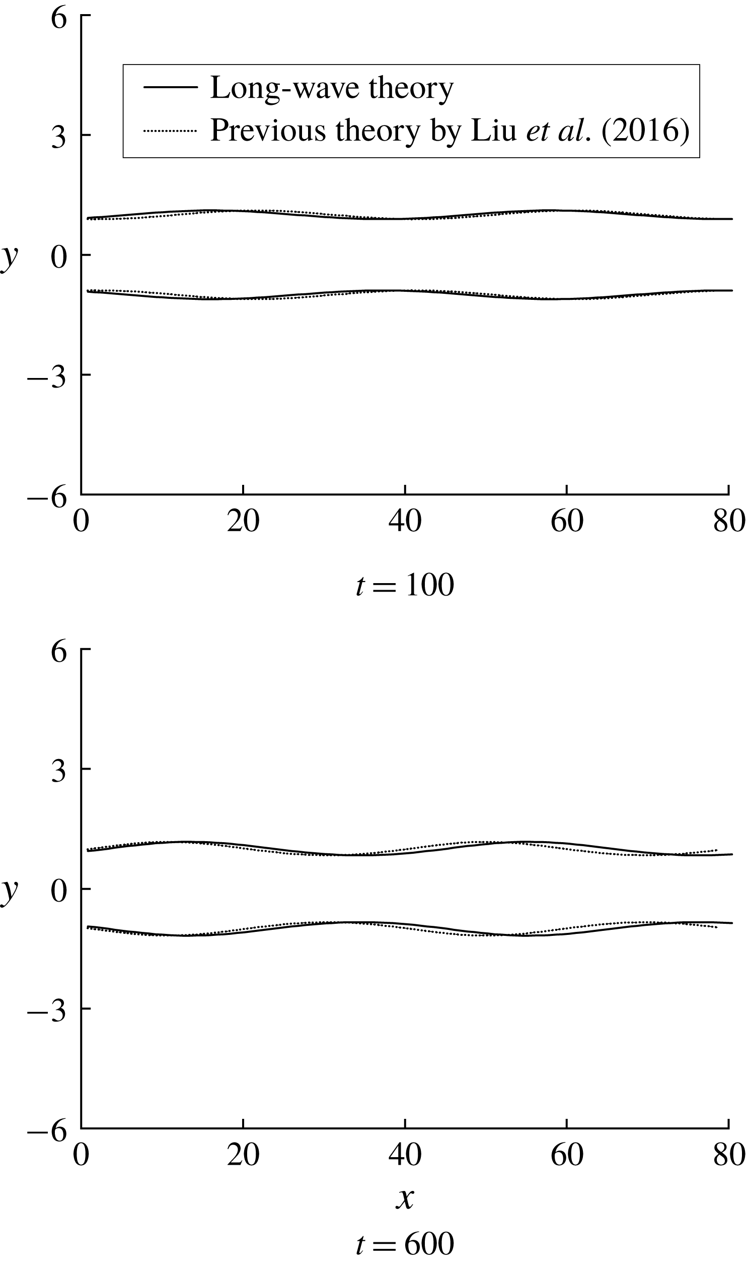
Figure 2 further depicts a comparison between the long-wave theoretical result and the theoretical result previously obtained by Liu et al. (Reference Liu, Yang and Ye2016) for the shape of interface deformation at two different dimensionless times,
 $t=100$
and
 $t=600$
, with other parameters set as
 $Re=1000$
,
 $We=200$
,
 $\bar{\unicode[STIX]{x1D70C}}=0.001$
and
 $\unicode[STIX]{x1D702}_{0}=0.1$
. With the given parameters, the dominant wavenumber was set as 0.15 in the long-wave theory, while it was 0.16 in the previous theory of Liu et al. (Reference Liu, Yang and Ye2016), which implies the long-wave assumption slightly changes the value of the dominant wavenumber obtained from the linear stability analysis. This also explains why there exist small differences between long-wave theoretical wave patterns at the interfaces and the previous theoretical ones obtained by Liu et al. (Reference Liu, Yang and Ye2016) in figure 2. Despite these tiny differences, the two theories are in good agreement with each other concerning the shape of interface deformation for the Newtonian liquid sheets.
Comparison between the long-wave theoretical result and the theoretical result previously obtained by Liu et al. (Reference Liu, Yang and Ye2016) for the shape of interface deformation at two different times (
 $Re=1000$
,
 $We=200$
,
 $\bar{\unicode[STIX]{x1D70C}}=0.001$
,
 $\unicode[STIX]{x1D702}_{0}=0.1$
).

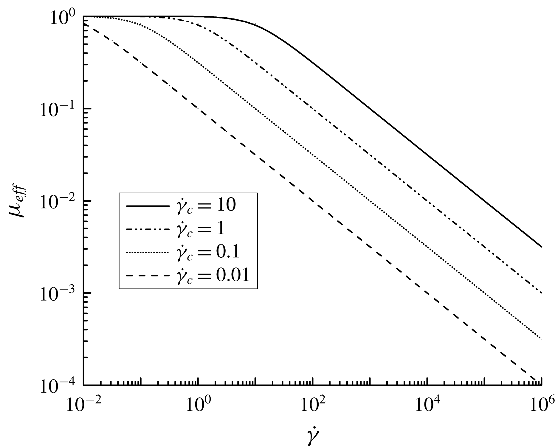
Viscosity
 $\unicode[STIX]{x1D707}_{eff}$
of dimensionless Carreau-law model versus shear rate
 $\dot{\unicode[STIX]{x1D6FE}}$
for
 $n=0.5$
.

4.2 Power-law case
From (3.14)–(3.27), it can be inferred that:
(1) When
 $D_{var}(2\unicode[STIX]{x1D714}_{1},2k_{1})=0$
, there would be singularities appearing in the solution of
$\hat{\unicode[STIX]{x1D702}}_{21}$
. Liu et al. (Reference Liu, Yang and Ye2016) presented an explanation of the similar singularity appearing in the expression of the second-order amplitude for Newtonian liquid sheets. Here, that explanation also works. When
$D_{var}(2\unicode[STIX]{x1D714}_{1},2k_{1})=0$
, since
$D_{var}(\unicode[STIX]{x1D714}_{25},2k_{1})=0$
in (3.21), it can be concluded that
$\unicode[STIX]{x1D714}_{25}=2\unicode[STIX]{x1D714}_{1}$
at these points. Then, because the dominant second-order disturbance amplitude (terms involving
$\hat{\unicode[STIX]{x1D702}}_{j21}$
) is in proportion to
$(\text{e}^{-2\text{i}\unicode[STIX]{x1D714}_{1}t}-\text{e}^{-\text{i}\unicode[STIX]{x1D714}_{25}t})$
, the dominant second-order amplitude tends to be zero and its influence of the second order would disappear. Besides, at these points, the current solution is not available and has no sense any more. Hence, the discussion below will ignore these singular points.
(2) For the Carreau liquid sheets studied here, the critical shear rate
$\dot{\unicode[STIX]{x1D6FE}}_{c}$
should be as small as possible. Since
$\dot{\unicode[STIX]{x1D6FE}}_{c}=\unicode[STIX]{x1D702}_{0}^{1/2}\unicode[STIX]{x1D6E4}_{1/2}$
,
$\unicode[STIX]{x1D6E4}_{1/2}$
should also be as small as possible at a magnitude of order unity. When
$\unicode[STIX]{x1D6E4}_{1/2}$
is small enough, the effect of shear-thinning would become evident.(3) The final expression of the second-order disturbance amplitude implies that the power-law factor
$n$
only impacts on terms involving
$\hat{\unicode[STIX]{x1D702}}_{j23}$
,
$\hat{\unicode[STIX]{x1D702}}_{j24}$
,
$\hat{\unicode[STIX]{x1D702}}_{j27}$
and
$\hat{\unicode[STIX]{x1D702}}_{j28}$
; that is, the power-law factor
$n$
affects the wave instability of harmonic waves of the fundamental wavelength or one third the fundamental wavelength.


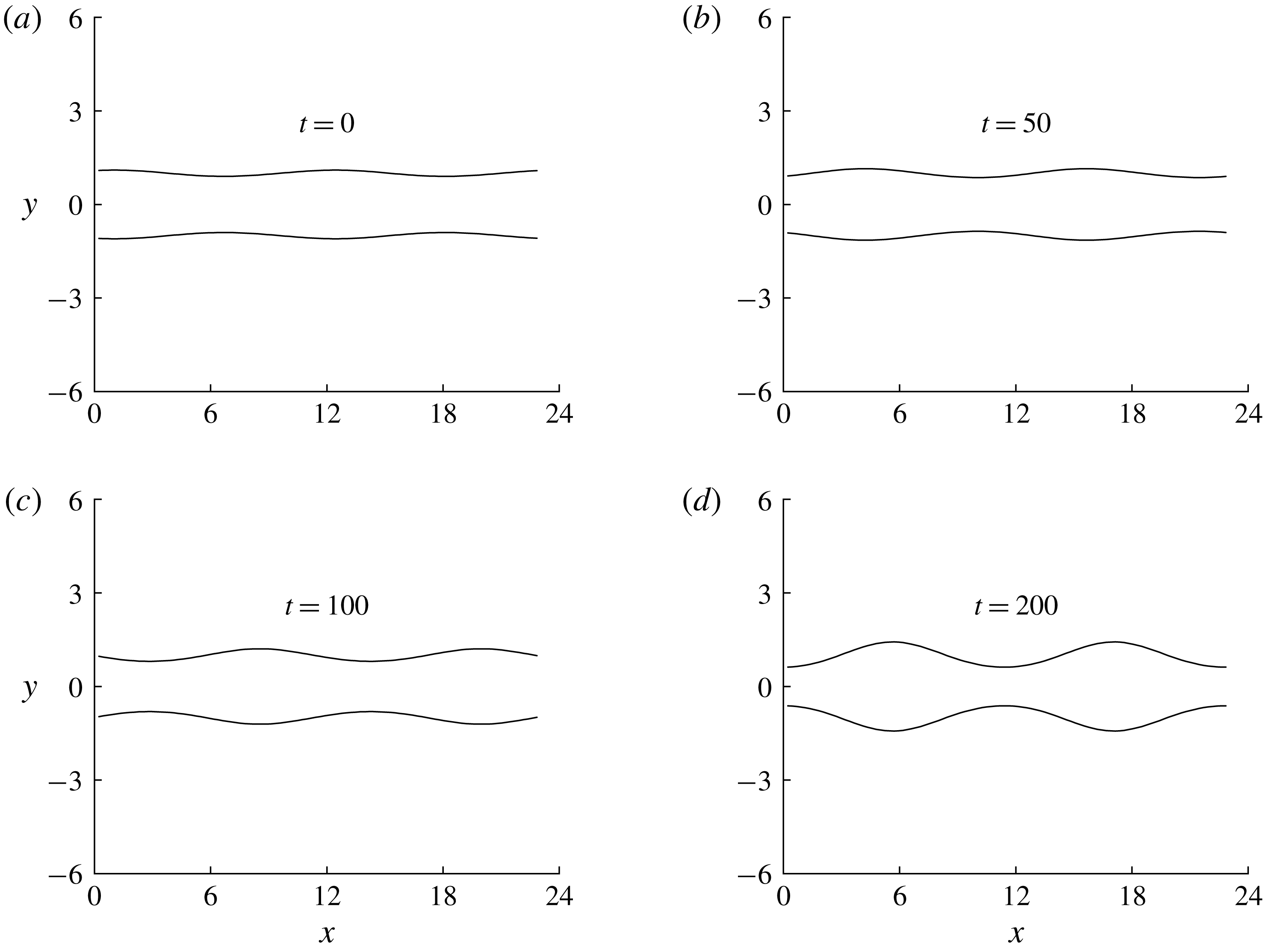
Evolution of waveform for power-law liquid sheets (
 $\unicode[STIX]{x1D70C}_{l}=995~\text{kg}~\text{m}^{-3}$
,
 $U=20~\text{m}~\text{s}^{-1}$
,
 $a=0.1~\text{mm}$
,
 $\unicode[STIX]{x1D70E}=0.065~\text{N}~\text{m}^{-1}$
,
 $\dot{\unicode[STIX]{x1D6FE}}_{c}=0.05~\text{s}^{-1}$
,
 $\bar{\unicode[STIX]{x1D70C}}=0.0012$
,
 $\unicode[STIX]{x1D702}_{0}=0.1$
,
 $k_{1}=0.55$
,
 $n=0.34$
).

For the non-dimensional Carreau-law model here, if the power-law index
 $n$
is set to be 0.5, the relation between the effective viscosity
 $\unicode[STIX]{x1D707}_{eff}$
and shear rate
 $\dot{\unicode[STIX]{x1D6FE}}$
can be demonstrated in figure 3. It shows four different cases with
 $\dot{\unicode[STIX]{x1D6FE}}_{c}=10$
, 1, 0.1 and 0.01, and it is evident that when the shear rate
 $\dot{\unicode[STIX]{x1D6FE}}$
increases from 0.01 to 10 000, the effective viscosity
 $\unicode[STIX]{x1D707}_{eff}$
has a greater decrease with a lower
 $\unicode[STIX]{x1D6FE}_{c}$
, which indicates that the shear-thinning effect is more pronounced for lower values of critical shear rate
 $\dot{\unicode[STIX]{x1D6FE}}_{c}$
.
In the following, the influence of power-law characteristics on liquid sheet instability is further analysed by waveform diagram. Figure 4 illustrates the evolution of waveform for power-law liquid sheets, with other parameters fixed at
 $\unicode[STIX]{x1D70C}_{l}=995~\text{kg}~\text{m}^{-3}$
,
 $U=20~\text{m}~\text{s}^{-1}$
,
 $a=0.1~\text{mm}$
,
 $\unicode[STIX]{x1D70E}=0.065~\text{N}~\text{m}^{-1}$
,
 $\dot{\unicode[STIX]{x1D6FE}}_{c}=0.05~\text{s}^{-1}$
,
 $\bar{\unicode[STIX]{x1D70C}}=0.0012$
,
 $\unicode[STIX]{x1D702}_{0}=0.1$
,
 $k_{1}=0.55$
and
 $n=0.34$
. It can be seen that as the dimensionless time
 $t$
increases, the amplitude of the surface wave also increases, with the upper surface and lower surface staying symmetric. At
 $t=200$
, there appears an obvious distortion on the surface wave, which manifests the influence of nonlinear properties. With time going on, the amplitude of the disturbance wave on the upper and lower surfaces of the liquid sheet becomes larger and larger. When the two interfaces are contacted, the liquid sheet will burst into many liquid filaments.
In order to investigate effects of the Carreau-law parameters in (2.4) on the second-order disturbance amplitude at the interfaces, a new parameter
 $B_{p}=\unicode[STIX]{x1D6E4}_{1/2}/\sqrt{1-n}=\dot{\unicode[STIX]{x1D6FE}}_{c}/\unicode[STIX]{x1D702}_{0}^{1/2}\sqrt{1-n}$
has been introduced. Then (3.25) can be rewritten as
 $$\begin{eqnarray}\displaystyle \unicode[STIX]{x1D702}_{j2} & = & \displaystyle \hat{\unicode[STIX]{x1D702}}_{j21}\cdot \text{e}^{2\text{i}k_{1}x}(\text{e}^{-2\text{i}\unicode[STIX]{x1D714}_{1}t}-\text{e}^{-\text{i}\unicode[STIX]{x1D714}_{25}t})+\hat{\unicode[STIX]{x1D702}}_{j23}\cdot \text{e}^{3\text{i}k_{1}x}(\text{e}^{-3\text{i}\unicode[STIX]{x1D714}_{1}t}-\text{e}^{-\text{i}\unicode[STIX]{x1D714}_{27}t})\nonumber\\ \displaystyle & & \displaystyle +\,\hat{\unicode[STIX]{x1D702}}_{j24}\cdot \text{e}^{\text{i}k_{1}x}(\text{e}^{-\text{i}\unicode[STIX]{x1D714}_{1r}t+3\unicode[STIX]{x1D714}_{1i}t}-\text{e}^{-\text{i}\unicode[STIX]{x1D714}_{1}t})+\text{c.c.},\end{eqnarray}$$
where
 $$\begin{eqnarray}\hat{\unicode[STIX]{x1D702}}_{j21}=(-1)^{\,j+1}\frac{2\text{i}Re(\unicode[STIX]{x1D714}_{1}-k_{1})^{2}-8{k_{1}}^{2}(\unicode[STIX]{x1D714}_{1}-k_{1})-\text{i}k_{1}{\unicode[STIX]{x1D714}_{1}}^{2}\bar{\unicode[STIX]{x1D70C}}Re\,\text{sgn}(k_{1})+\text{i}{k_{1}}^{4}\unicode[STIX]{x1D6E4}}{\text{i}k_{1}ReD_{var}(2\unicode[STIX]{x1D714}_{1},2k_{1})}{\hat{\unicode[STIX]{x1D702}}_{j1}}^{2},\end{eqnarray}$$
 $$\begin{eqnarray}\hat{\unicode[STIX]{x1D702}}_{j23}=(-1)^{\,j+1}\frac{-8{k_{1}}^{2}(\unicode[STIX]{x1D714}_{1}-k_{1})^{3}}{{B_{p}}^{2}[12k_{1}^{2}(\unicode[STIX]{x1D714}_{1}-k_{1})-\text{i}Re(\unicode[STIX]{x1D714}_{1}-k_{1})^{2}+9\text{i}k_{1}^{4}\unicode[STIX]{x1D6E4}-3i{\unicode[STIX]{x1D714}_{1}}^{2}k_{1}\bar{\unicode[STIX]{x1D70C}}Re\,\text{sgn}(k_{1})]}{\hat{\unicode[STIX]{x1D702}}_{j1}}^{3},\end{eqnarray}$$
 $$\begin{eqnarray}\hat{\unicode[STIX]{x1D702}}_{j24}=(-1)^{\,j+1}\frac{-24{k_{1}}^{2}(\unicode[STIX]{x1D714}_{1}-k_{1})^{2}(\bar{\unicode[STIX]{x1D714}}_{1}-k_{1}){\hat{\unicode[STIX]{x1D702}}_{j1}}^{2}\bar{\hat{\unicode[STIX]{x1D702}}}_{j1}}{{B_{p}}^{2}[\text{i}Re\unicode[STIX]{x1D6EC}^{2}+4\text{i}k_{1}^{2}\unicode[STIX]{x1D6EC}+\text{i}k_{1}(3\unicode[STIX]{x1D714}_{1i}-i\unicode[STIX]{x1D714}_{1r})^{2}\bar{\unicode[STIX]{x1D70C}}Re\,\text{sgn}(k_{1})+\text{i}k_{1}^{4}\unicode[STIX]{x1D6E4}]}.\end{eqnarray}$$
It is evident that the terms containing
 $B_{p}$
in the expression of the second-order amplitude are only
 $\hat{\unicode[STIX]{x1D702}}_{j23}$
and
 $\hat{\unicode[STIX]{x1D702}}_{j24}$
. Therefore, we assume a criterion for judging the effect of power-law characteristics on the second-order disturbance amplitude: when the ratio of the second-order power-law and non-power-law amplitude intensity
 $\unicode[STIX]{x1D702}$
(
 $\unicode[STIX]{x1D702}=|\hat{\unicode[STIX]{x1D702}}_{23}(\text{e}^{3\unicode[STIX]{x1D714}_{1i}t}-\text{e}^{\unicode[STIX]{x1D714}_{27i}t})+\hat{\unicode[STIX]{x1D702}}_{24}(\text{e}^{3\unicode[STIX]{x1D714}_{1i}t}-\text{e}^{\unicode[STIX]{x1D714}_{1i}t})/\hat{\unicode[STIX]{x1D702}}_{21}(\text{e}^{2\unicode[STIX]{x1D714}_{1i}t}-\text{e}^{\unicode[STIX]{x1D714}_{25i}t})|$
) is more than 1, the influence of the second-order power-law amplitude can be at least comparable with that caused by the second-order non-power-law amplitude and then the shear-thinning effect on the second-order amplitude can be considered evident. Under this circumstance, given that
 $\unicode[STIX]{x1D70C}_{l}=995~\text{kg}~\text{m}^{-3}$
,
 $U=20~\text{m}~\text{s}^{-1}$
,
 $a=0.1~\text{mm}$
,
 $\unicode[STIX]{x1D70E}=0.065~\text{N}~\text{m}^{-1}$
,
 $\bar{\unicode[STIX]{x1D70C}}=0.0012$
,
 $\unicode[STIX]{x1D702}_{0}=0.01$
and
 $k_{1}=0.55$
, it can be calculated that
 $B_{p}$
should be less than 0.001388 to satisfy the assumed criterion. Since
 $0<n<1$
, it is easy to deduce that
 $\unicode[STIX]{x1D6E4}_{1/2}$
should be of the order of
 $10^{-3}$
. However, in (2.27), it is known that
 $\unicode[STIX]{x1D6E4}_{1/2}$
should be
 $O(1)$
, which is incompatible with the value obtained from the assumed criterion here. This implies that the ratio of the second-order power-law and non-power-law amplitude intensity
 $\unicode[STIX]{x1D702}$
is actually far less than 1, making the non-power-law amplitude dominant in the second-order disturbance amplitude.
The effects of the parameter
 $B_{p}$
and the Reynolds number
 $Re$
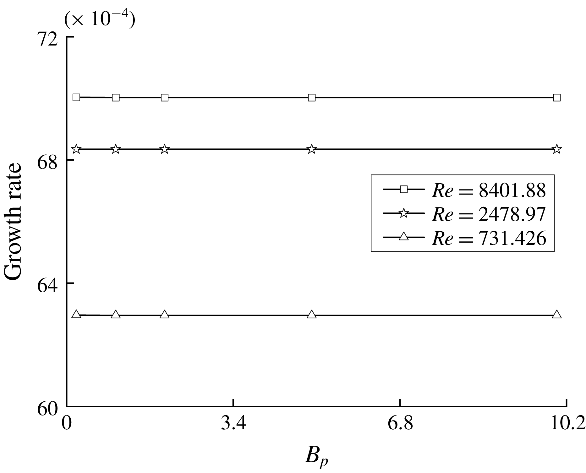
on the unstable growth rate of the disturbance amplitude at the interfaces were then investigated, as shown in figure 5. Each data point was obtained by fitting the average growth rate of the disturbance amplitude in 300 unit time. It can be seen that for each given Reynolds number, the growth rate is not sensitive to the variation of
 $B_{p}$
, and almost stays the same with the increase of
 $B_{p}$
. While for different Reynolds numbers, a higher
 $Re$
will lead to a larger growth rate for the power-law liquid sheets, and eventually accelerates the rupture process of the liquid sheets.
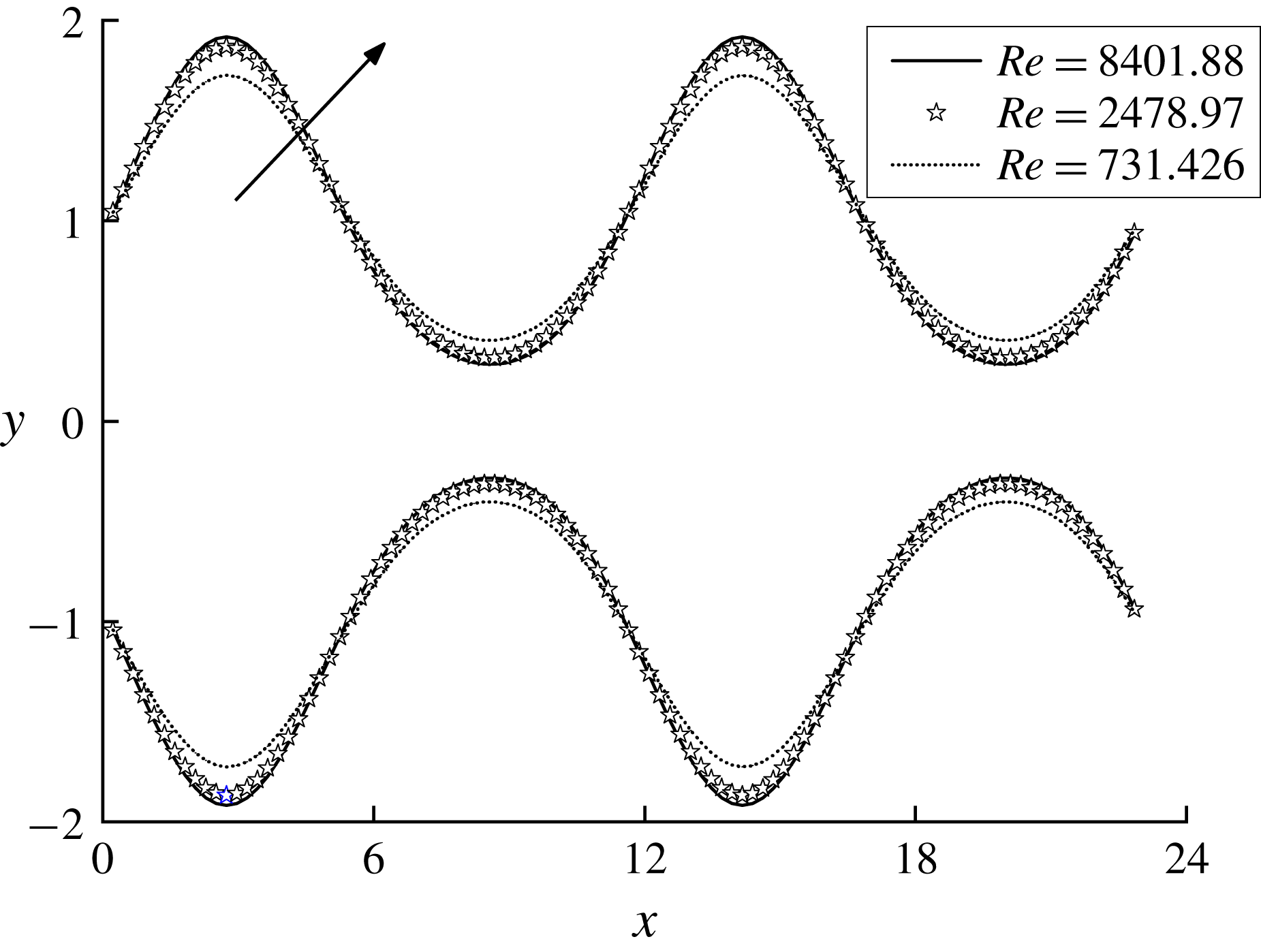
Figure 6 demonstrates the effect of the Reynolds number
 $Re$
on the interface wave pattern for
 $B_{p}=1$
and
 $t=300$
. It indicates that when
 $Re$
becomes larger, the disturbance amplitude at the interfaces will increase, and the gap between the upper and lower interfaces will become smaller. And the two interfaces in turn become more distorted, resulting in flatter ligaments when the liquid sheets finally break up.
The growth rate versus
 $B_{p}$
at different Reynolds numbers.

Effect of
 $Re$
on the interface wave pattern for
 $B_{p}=1$
and
 $t=300$
.

5 Numerical observation
In view of the two-variable equations (2.23)–(2.24), numerical solutions have been calculated by the method of finite difference. Introducing two variables
 $h$
and
 $q$
, replacing
 $\unicode[STIX]{x1D702}_{j}$
with
 $h$
and letting
 $q=(1+\unicode[STIX]{x1D702}_{j})u$
, then the long-wave model equations can be rewritten as follows:
 $$\begin{eqnarray}h_{t}+q_{x}=0,\end{eqnarray}$$
 $$\begin{eqnarray}\displaystyle Re\left[q_{t}+\frac{(q^{2})_{x}}{h}-\frac{q^{2}h_{x}}{h^{2}}\right] & = & \displaystyle 4\left[h\left(\frac{q}{h}\right)_{x}\right]_{x}\left[1+4\left(\frac{(q/h)_{x}}{\dot{\unicode[STIX]{x1D6FE}_{c}}}\right)^{2}\right]^{(n-1)/2}\nonumber\\ \displaystyle & & \displaystyle +\,\frac{16(n-1)}{{\dot{\unicode[STIX]{x1D6FE}}_{c}}^{2}}h\left[\left(\frac{q}{h}\right)_{x}\right]^{2}\left(\frac{q}{h}\right)_{xx}\left[1+4\left(\frac{(q/h)_{x}}{\dot{\unicode[STIX]{x1D6FE}_{c}}}\right)^{2}\right]^{(n-3)/2}\nonumber\\ \displaystyle & & \displaystyle +\,\bar{\unicode[STIX]{x1D70C}}Reh{\mathcal{H}}[h_{tt}]+h\unicode[STIX]{x1D6E4}h_{xxx}.\end{eqnarray}$$
The Runge–Kutta method is used to integrate in the time direction. While in the spatial direction, discrete markers on the interfaces are utilized:
 $$\begin{eqnarray}x_{n}=2\unicode[STIX]{x03C0}n/kN,\quad n=0,1,2,\ldots ,N-1,\end{eqnarray}$$
where
 $N$
is the number of markers within one wavelength on the upper interface.
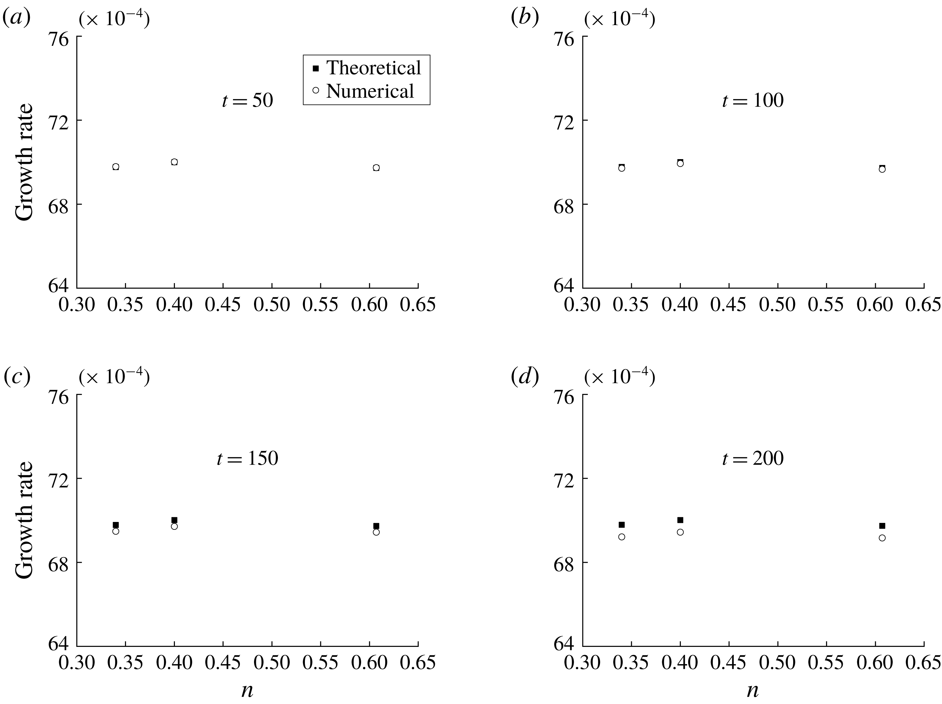
To verify the validity of the weakly nonlinear analysis, comparisons between the analytical growth rate of the instability and numerical growth rate at different times have been made, as shown in figure 7. It indicates that at early stages of the disturbance, the growth rates of the instability obtained by weakly nonlinear analysis and by the numerical method keep in agreement with each other for all the three fluids (1, 2 and 3) mentioned above, which proves the correctness of the weakly nonlinear analysis conducted for small perturbations. With an increase of time, when the dimensionless time
 $t=150$
, there is a slight difference between the two. As time goes on, the difference increases (
 $t=200$
). This is because during the later development period of the disturbance waves, with time increasing, the disturbance amplitude at the interface becomes very large and the rupture of liquid sheets near the breakup time is actually a strong nonlinear process. This implies that the weakly nonlinear analysis conducted here for the power-law liquid sheets can predict well the interface shape of disturbance waves at the initial stages, but fails to illustrate the accurate waveform at liquid–gas interfaces near the rupture point.
Comparison between numerical simulation and analytical results for growth rate at different times for three kinds of power-law liquid sheets: fluid 1,
 $n=0.34$
; fluid 2,
 $n=0.4$
; fluid 3,
 $n=0.607$
(
 $\unicode[STIX]{x1D70C}_{l}=995~\text{kg}~\text{m}^{-3}$
,
 $U=20~\text{m}~\text{s}^{-1}$
,
 $a=0.1~\text{mm}$
,
 $\unicode[STIX]{x1D70E}=0.065~\text{N}~\text{m}^{-1}$
,
 $\bar{\unicode[STIX]{x1D70C}}=0.0012$
,
 $\unicode[STIX]{x1D702}_{0}=0.1$
,
 $k_{1}=0.55$
).

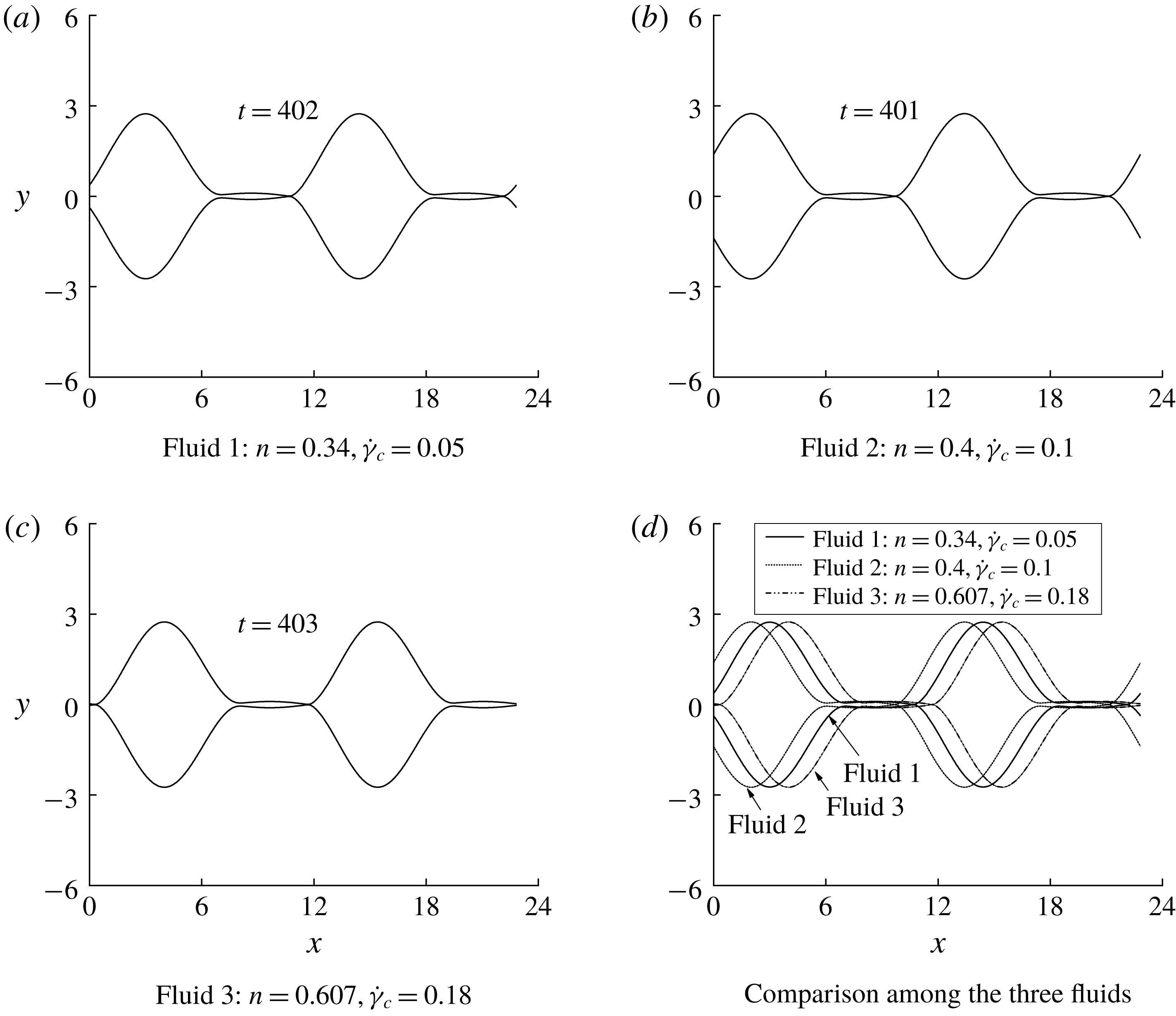
Numerical solutions of interface deformation at breakup time for three different kinds of fluids (
 $\unicode[STIX]{x1D70C}_{l}=995~\text{kg}~\text{m}^{-3}$
,
 $U=20~\text{m}~\text{s}^{-1}$
,
 $a=0.1~\text{mm}$
,
 $\unicode[STIX]{x1D70E}=0.065~\text{N}~\text{m}^{-1}$
,
 $\bar{\unicode[STIX]{x1D70C}}=0.0012$
,
 $\unicode[STIX]{x1D702}_{0}=0.1$
,
 $k_{1}=0.55$
).

Numerical simulation of waveform evolution for power-law liquid sheets (
 $\unicode[STIX]{x1D70C}_{l}=995~\text{kg}~\text{m}^{-3}$
,
 $U=20~\text{m}~\text{s}^{-1}$
,
 $a=0.1~\text{mm}$
,
 $n=0.34$
,
 $\dot{\unicode[STIX]{x1D6FE}}_{c}=0.05~\text{s}^{-1}$
,
 $\unicode[STIX]{x1D70E}=0.065~\text{N}~\text{m}^{-1}$
,
 $\bar{\unicode[STIX]{x1D70C}}=0.0012$
,
 $\unicode[STIX]{x1D702}_{0}=0.1$
,
 $k_{1}=0.55$
).

Time evolution of the maximum displacement of disturbance waves at upper interface
 $\unicode[STIX]{x1D702}_{1max}$
for power-law liquid sheets (
 $\unicode[STIX]{x1D70C}_{l}=995~\text{kg}~\text{m}^{-3}$
,
 $U=20~\text{m}~\text{s}^{-1}$
,
 $a=0.1~\text{mm}$
,
 $\unicode[STIX]{x1D70E}=0.065~\text{N}~\text{m}^{-1}$
,
 $\bar{\unicode[STIX]{x1D70C}}=0.0012$
,
 $\unicode[STIX]{x1D702}_{0}=0.1$
,
 $k_{1}=0.55$
,
 $n=0.34$
,
 $\dot{\unicode[STIX]{x1D6FE}}_{c}=0.05~\text{s}^{-1}$
).

In the following, the numerical solution is used to compensate for the defect of weakly nonlinear stability analysis. Table 1 gives data of three typical xanthan gum solutions in water with their rheological parameters (data from Ruyer-Quil et al.
Reference Ruyer-Quil, Chakraborty and Dandapat2012), in which
 $\unicode[STIX]{x1D707}_{n}$
represents the consistency coefficient and
 $\unicode[STIX]{x1D707}_{0}$
indicates the dynamic viscosity at zero shear rate. Surface tension and density are respectively
 $\unicode[STIX]{x1D70E}=0.065~\text{N}~\text{m}^{-1}$
and
 $\unicode[STIX]{x1D70C}_{l}=995~\text{kg}~\text{m}^{-3}$
. Figure 8 displays the shape of interface deformation at breakup time for fluids 1, 2 and 3, with other parameters fixed at
 $\unicode[STIX]{x1D70C}_{l}=995~\text{kg}~\text{m}^{-3}$
,
 $U=20~\text{m}~\text{s}^{-1}$
,
 $a=0.1~\text{mm}$
,
 $\unicode[STIX]{x1D70E}=0.065~\text{N}~\text{m}^{-1}$
,
 $\bar{\unicode[STIX]{x1D70C}}=0.0012$
,
 $\unicode[STIX]{x1D702}_{0}=0.1$
and
 $k_{1}=0.55$
. It can be concluded that when
 $n$
varies from 0.34 to 0.607, the breakup time decreases first (from 402 to 401) and then increases (from 401 to 403). Evidently, the wave diagram at breakup time remains analogous as
 $\dot{\unicode[STIX]{x1D6FE}}_{c}$
varies from 0.05 to
 $0.18~\text{s}^{-1}$
; each of them is just of different phases. Therefore, in the next step, we choose fluid 1 (
 $n=0.34$
,
 $\dot{\unicode[STIX]{x1D6FE}}_{c}=0.05~\text{s}^{-1}$
) as the research object to further study the whole process for power-law liquid sheets from the beginning of the disturbance to the final rupture.
Three typical xanthan gum solutions in water with their rheological parameters (data from Ruyer-Quil et al. Reference Ruyer-Quil, Chakraborty and Dandapat2012).

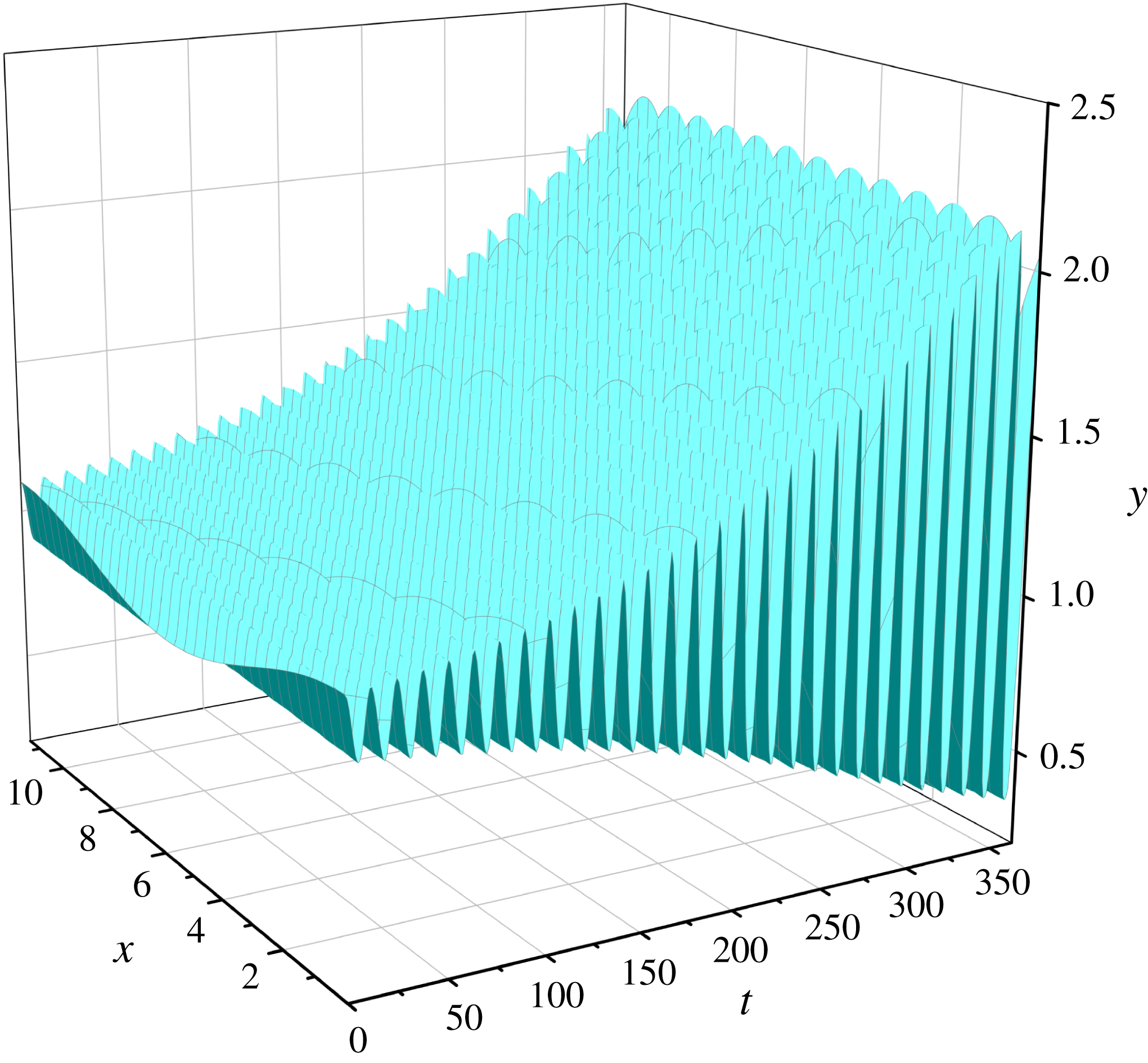
Figure 9 displays the numerical simulation of waveform evolution for power-law liquid sheets under the typical situation of fluid 1. It can be clearly seen that the disturbance wave develops over time and oscillates periodically in space, which is indeed the characteristic of temporal stability analysis. As the dimensionless time
 $t$
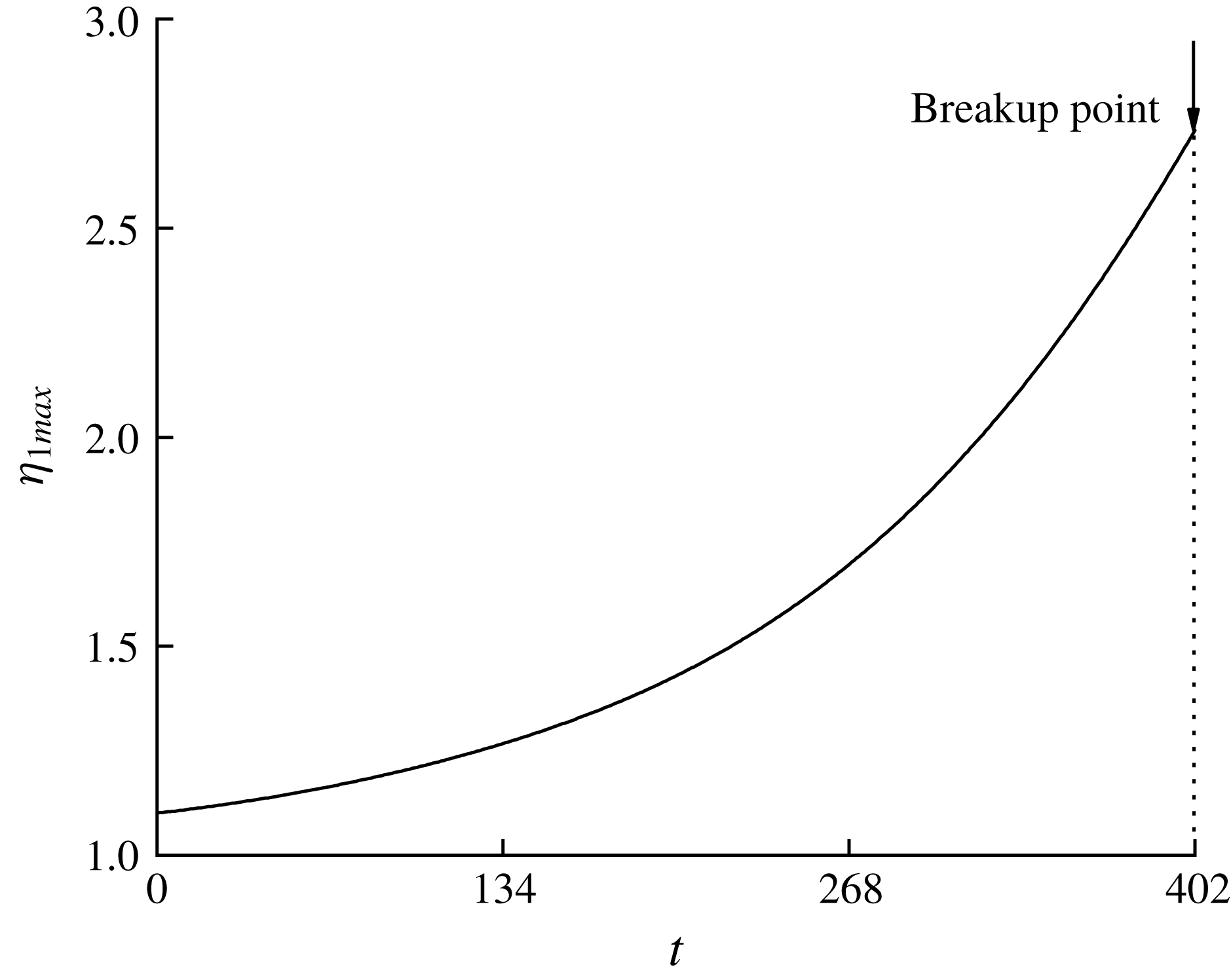
goes on, the disturbance wave amplitude of the liquid–gas interface increases, which can also be concluded from figure 10. At
 $t=402$
, the disturbance wave amplitude is large enough to make the upper and lower surfaces touch each other and the sheets would break up into many liquid filaments eventually. During the whole process, the time evolution of the maximum displacement
 $\unicode[STIX]{x1D702}_{1max}$
of disturbance waves at the upper interface is also presented in figure 10.
6 Conclusions
In this paper, weakly nonlinear wave evolution of power-law liquid sheets has been investigated under the disturbances of varicose mode. The conclusions can be drawn as follows.
The final expression of the second-order disturbance amplitude shows that the power-law factor
 $n$
has an effect on the instability of those harmonic waves with the fundamental wavelength or one third the fundamental wavelength.
Concerning the influence of the Carreau-law rheological parameter
 $B_{p}$
, the unstable growth rate of the disturbance amplitude is almost unchanged with the variation of
 $B_{p}$
. As for the Reynolds number, with time going on, a larger
 $Re$
will result in higher disturbance amplitude and more distorted interfaces, promoting the breakup of liquid sheets.
In the initial phase of wave evolution, concerning the unstable growth rate, there is good agreement between numerical simulations and analytical results, verifying that the weakly nonlinear analysis conducted here is useful for small perturbations. When the time is approaching the breakup time, weakly nonlinear stability theory fails to predict the accurate waveform at the interfaces. The numerical simulation is needed to compensate for the defect and to depict the accurate wave pattern near the rupture point.
Acknowledgements
The authors would like to thank Professor N. J. Balmforth for his warm guidance and discussion concerning that part of the theoretical analysis presented in §§ 2 and 3. Also, the authors would like to acknowledge the help and the support given by Dr Y. Liu, Dr C. Mo and Dr T. Hu in the aspect of numerical methods and Matlab code. The financial support of the National Natural Science Funds for Distinguished Young Scholar (grant no. 11525207) and National Nature Science Foundation of China (grant no. 11272036 and 11672025) is gratefully acknowledged.