



1. Introduction
The transit of a concentrated load across a floating ice sheet induces a complex coupling between the flexural response of the solid cover and the underlying fluid hydrodynamics. Within the framework of classical linear theory, the steady-state deflection is predicted to become singular as the load speed
 $c$
approaches the critical speed
 $c_m$
, defined by the minimum of the phase velocity. While nonlinearities, frequently captured via the forced nonlinear Schrödinger (fNLS) equation, provide a mechanism to regularise this singularity (Părău & Dias Reference Plotnikov and Toland2002), they alone do not account for the observed spatial symmetry breaking. Experimental observations (Squire et al. Reference Squire, Robinson, Langhorne and Haskell1988; Takizawa Reference Takizawa1988) consistently reveal a distinct downstream lag of the maximum ice deflection relative to the load position. Particularly within the small-amplitude, steady-state and subcritical loading regime (resembling the slow-moving loads in Takizawa Reference Takizawa1988), the persistence of this localised offset highlights the critical role of dissipative mechanisms in faithfully capturing both the characteristic response peak and the underlying energy–flux balance.
(a) Schematic of an S-shaped bifurcation curve for hydroelastic waves under a moving load. (b) Bifurcation diagram of a forced–damped Duffing oscillator.

When dissipation and nonlinearity are of comparable order, the hydroelastic response in the present two-dimensional system exhibits a characteristic S-shaped bifurcation structure, a hallmark of forced–dissipative nonlinear systems (figure 1
 $a$
). This behaviour finds a direct dynamical analogue in the forced–damped Duffing-type oscillator (figure 1
 $b$
), wherein the interplay between external forcing, nonlinear restoration and damping gives rise to fold bifurcations and hysteretic jump phenomena (see e.g. figures 1–5 in Nayfeh & Mook Reference Nayfeh and Mook1995). In the context of hydroelastic waves, the moving load acts as a resonant drive, inducing a bistable regime bounded by two critical speeds,
 $c_1$
and
 $c_2$
, also referred to as ‘limit points’ where the solution branch turns and stability changes (Calvo & Akylas Reference Calvo and Akylas2002). As the load speed is increased monotonically, the response undergoes a discontinuous upward transition at the fold point
 $c_1$
, shifting to a high-amplitude state characterised by a solitary-wave-like profile (see the transition in figures 6
a,b). Conversely, a quasi-static reduction in speed leads to the abrupt collapse of this solution branch at the lower limit
 $c_2$
, marking the return to a small-amplitude state (figures 6
c,d).
Although such bifurcation structures have been identified within simplified models (Cho & Akylas Reference Cho and Akylas2009), a complete characterisation of the hydroelastic response necessitates a fully nonlinear potential-flow framework. While numerical continuation has successfully traced solitary-wave branches in various nonlinear dispersive systems (e.g. Vanden-Broeck & Dias Reference Vanden-Broeck and Dias1992; Părău & Dias Reference Plotnikov and Toland2002; Guyenne & Părău Reference Guyenne and Părău2012; Gao et al. Reference Gao, Wang and Milewski2019; Hu & Wang Reference Hu and Wang2025), existing formulations typically neglect dissipation, thereby failing to capture the experimentally observed spatial symmetry breaking and downstream lag of wave profiles. Indeed, the simultaneous presence of moving loads and dissipative mechanisms destroys the translational invariance and symmetry of travelling-wave solutions, properties that underpin the classical speed–energy bifurcation framework. Consequently, the conventional critical- or limit-point criterion for the exchange of stability (Saffman Reference Saffman1985) is no longer applicable in this regime. To address these challenges, we first employ a conformal-mapping formulation to resolve both the steady and unsteady responses of the system under combined forcing and dissipation. Nevertheless, the underlying dynamical essence, specifically the mechanisms of stability exchange and steady-state selection, remains largely obscured within the infinite-dimensional phase space of the governing partial differential equations (Pelinovsky & Grimshaw Reference Părău and Dias1997). This motivates the development of a reduced-order model that uncovers this dynamical structure in a mathematically tractable and physically transparent manner.
To elucidate the universal mathematical structure underlying the hydroelastic response, we reduce the governing equations to their primary degrees of freedom: the wave amplitude and the spatial lag. By projecting the infinite-dimensional dynamical system onto a two-dimensional manifold, we establish a formal connection between the moving-load problem and the forced–damped Duffing oscillator. This reduction reveals that the spatial lag is not merely a passive geometric offset, but rather the hydrodynamic analogue of a temporal phase shift, which the system adjusts spontaneously to achieve phase-locking with the moving load. Such a framework provides a theoretical basis for the stability exchange observed in numerical simulations, and characterises the global S-shaped structure of the bifurcation diagram, identifying the power-balance condition as the selection criterion for steady states.
The remainder of the paper is organised as follows. In § 2, the governing equations are formulated within a fully nonlinear conformal-mapping framework. The bifurcation structures of steady-state solutions and their corresponding linear stability characteristics are presented in § 3. A theoretical dissection of the limit points
 $c_1$
and
 $c_2$
is provided in § 4, utilising both fNLS theory and a global energy-balance approach to bridge the numerical and analytical results. In § 5, we develop a reduced-order model to elucidate the structural correspondence between the hydroelastic response and the forced–damped Duffing oscillator. Finally, the principal findings and potential extensions are discussed in §§ 6 and 7, respectively.
2. Mathematical formulations
We consider the two-dimensional motion of an inviscid, incompressible fluid of uniform depth
 $H$
, bounded above by a thin ice sheet, as illustrated in figure 2. A Cartesian coordinate system
 $(x,y)$
is adopted, where the
 $x$
-axis coincides with the undisturbed ice–water interface, and the
 $y$
-axis points vertically upwards. The deflection of the ice-covered surface is denoted by
 $y=\zeta (x,t)$
, where
 $t$
represents time. Assuming the flow to be irrotational, the velocity field can be represented as the spatial gradient of a potential function
 $\phi (x,y,t)$
. Mass conservation for an incompressible fluid then requires
 $\phi$
to be harmonic, satisfying the Laplace equation
 \begin{equation} \phi _{xx}+\phi _{yy}=0\quad \text{for} \quad {-H}\lt y\lt \zeta (x,t), \end{equation}
with the impermeability boundary condition at the rigid bottom given by
 \begin{equation} \phi _y=0 \quad \text{at} \quad y=-H, \end{equation}
where the subscripts indicate differentiation with respect to the corresponding variables. The fluid dynamics is coupled to the ice cover through the kinematic and dynamic boundary conditions at
 $y=\zeta (x,t)$
, expressed respectively as
 \begin{gather} \zeta _t=\phi _y-\zeta _x\phi _x, \end{gather}
 \begin{gather} \rho \left (\phi _t+\frac 12|\boldsymbol{\nabla }\phi |^2+g\zeta \right )+P_w=0, \end{gather}
where
 $g$
is the acceleration due to gravity,
 $\rho$
is the fluid density, and
 $\boldsymbol{\nabla }=(\partial _x,\partial _y)$
represents the two-dimensional gradient operator. The term
 $P_w$
represents the excess pressure exerted by the ice cover, the specific form of which is determined by the constitutive model of the ice.
A schematic description of the hydroelastic wave system in Cartesian coordinates.

The ice cover is modelled as an elastic plate governed by the Cosserat shell theory of Plotnikov & Toland (Reference Pelinovsky and Grimshaw2011), which accommodates large-amplitude deformations through a geometrically invariant formulation (Guyenne & Părău Reference Guyenne and Părău2012). To account for energy dissipation, we incorporate a linear damping term. While viscoelastic constitutive models are often regarded as more mechanistically robust (Squire et al. Reference Squire, Hosking, Kerr and Langhorne1996; Zhestkaya Reference Zhestkaya1999), the present linear formulation is motivated by its consistency with the power-law attenuation observed in ice-covered seas (Meylan et al. Reference Meylan, Bennetts, Mosig, Rogers, Doble and Peter2018) and its proven efficacy in regularising wave amplitudes (Dinvay et al. Reference Dinvay, Kalisch and Părău2019; Cheng & Wang Reference Cheng and Wang2026). Such a simplification enhances numerical tractability while retaining the critical dynamical features, including the bifurcation manifold, stability transitions, and the primary nonlinear characteristics of the system. The dynamic balance of the ice plate is expressed as
 \begin{equation} D\left (\kappa _{ss}+\frac 12\kappa ^3\right )+b\zeta _{t}=-p(x-ct)+P_w, \end{equation}
where
 $D$
is the flexural rigidity,
 $b$
is the damping coefficient, and
 $\kappa$
and
 $s$
denote the curvature and arc-length coordinate of the ice–water interface, respectively. We note that the inertial term of the plate is omitted in (2.5). When the plate and fluid densities are comparable, the plate’s inertia can be neglected provided that the wavelength is much larger than the plate thickness, as is typically the case in sea–ice environments (Takizawa Reference Takizawa1985). The term
 $p(x-ct)$
represents the pressure distribution of the load moving at a constant speed
 $c$
, defined as positive when acting downwards on the plate surface.
Substituting the expression for
 $P_w$
from the plate-balance equation (2.5) into the Bernoulli equation (2.4) yields the combined dynamic boundary condition at
 $y=\zeta (x,t)$
:
 \begin{equation} \rho \left (\phi _t+\frac 12|\boldsymbol{\nabla }\phi |^2+g\zeta \right )+D\left (\kappa _{ss}+\frac 12\kappa ^3\right )+b\zeta _{t}+p(x-ct)=0. \end{equation}
Together with the Laplace equation (2.1), the bottom impermeability condition (2.2), and the kinematic boundary condition (2.3), this expression completes the closed system of equations governing the fully nonlinear hydroelastic wave problem.
For simplicity, we non-dimensionalise the primitive equations using
 \begin{equation} \left (\frac {D}{\rho g}\right )^{\frac{1}{4}},\quad \left (\frac {D}{\rho g^5}\right )^{\frac{1}{8}},\quad \left (\frac {D^3g}{\rho ^3}\right )^{\frac{1}{8}} \end{equation}
as the units of length, time and velocity potential, respectively. After this rescaling, (2.1)–(2.3) remain unchanged, while the dynamic boundary condition (2.6) is modified to
 \begin{equation} \phi _t+\frac 12|\boldsymbol{\nabla }\phi |^2+\zeta +\kappa _{ss}+\frac 12\kappa ^3+\mu \zeta _t+p(x-ct)=0, \end{equation}
where
 $\mu =b (D\rho ^7g^3 )^{-1/8}$
represents the non-dimensional damping coefficient. Equations (2.1)–(2.3) and (2.8) form a closed system for
 $\phi$
and
 $\zeta$
. The nonlinear behaviour originates from three sources: the kinematic convective term, the dynamic kinetic energy term, and the geometric nonlinearity of the plate model. In the linear limit, the model recovers the classical Rayleigh-type response.
Following the surface Euler system formalism (Dyachenko et al. Reference Dyachenko, Kuznetsov, Spector and Zakharov1996; Choi & Camassa Reference Choi and Camassa1999; Tiron & Choi Reference Tiron and Choi2012), we employ a time-dependent conformal mapping to transform the physical fluid domain into a uniform horizontal strip in the
 $\xi +\text{i}\eta$
plane, where the ice–water interface is mapped to the real axis
 $\eta =0$
. In a reference frame co-moving with the load at speed
 $c$
, the interface is parametrised as
 $(X(\xi ,t),Y(\xi ,t))$
, and the governing equations are formulated in terms of the surface velocity potential
 $\varPhi (\xi ,t)\equiv \phi (X,Y,t)-cX$
. The evolution of the system is then dictated by
 \begin{equation} Y_t =Y_\xi\, \mathcal{C}\left [\frac {\varPsi _\xi }{J}\right ]-X_\xi \,\frac {\varPsi _\xi }{J}, \end{equation}
 \begin{equation} \begin{aligned} \varPhi _t &= \frac {\varPsi _\xi ^2-\varPhi _\xi ^2}{2J}+\varPhi _\xi\, \mathcal{C}\left [\frac {\varPsi _\xi }{J}\right ]-Y-\frac 12\left [\frac {\kappa _{\xi \xi }}{J}+\left (\frac {\kappa _\xi }{J}\right )_\xi +\kappa ^3\right ]\\ &\quad-\mu \left (-\frac {\varPsi _\xi }{X_\xi } -c\,\frac {Y_\xi }{X_\xi }\right )-p(X)+\frac {c^2}{2}, \end{aligned} \end{equation}
where
 $J=X_\xi ^2+Y_\xi ^2$
is the Jacobian of the transformation,
 $\varPsi$
denotes the stream function at the free surface, and the interface curvature
 $\kappa$
in the conformal plane is expressed as
 \begin{equation} \kappa =\frac {X_\xi Y_{\xi \xi }-X_{\xi \xi }Y_\xi }{J^{3/2}}. \end{equation}
The pseudo-differential operator
 $\mathcal{C}$
relates the surface variables to their harmonic conjugates, and is defined in Fourier space by the multiplier
 $\text{i}\coth (k\widetilde {H})$
, where
 $\widetilde {H}=\hat {Y}_0+H$
represents the mean depth of the conformal strip, with
 $\hat {Y}_0$
denoting the spatial average of
 $Y$
. The mapping is closed by the conjugate relations
 \begin{equation} \varPhi _\xi = \boldsymbol{\mathcal{U}}-c-\mathcal{C}\left [\varPsi _\xi \right ]\!,\quad X=\xi -\mathcal{C}[Y], \end{equation}
where
 $\mathcal{U}$
is the wave-induced mean horizontal velocity; interested readers are referred to Gao et al. (Reference Gao, Wang and Milewski2019) and Hu & Wang (Reference Hu and Wang2025) for a comprehensive derivation. Setting the time derivatives in (2.9)–(2.10) to zero yields the steady-state equation
 \begin{equation} -\frac {c^2}{2}+\frac {(\boldsymbol{\mathcal{U}}-c)^2}{2J}+Y+\frac 12\left [\frac {\kappa _{\xi \xi }}{J}+\left (\frac {\kappa _\xi }{J}\right )_\xi +\kappa ^3\right ]+c\mu \frac {Y_\xi }{X_\xi }+p(X)=0, \end{equation}
subject to the constraints
 $X=\xi -\mathcal{C}[Y]$
,
 $\varPhi _\xi = \boldsymbol{\mathcal{U}}-c$
and
 $\varPsi _\xi =0$
. Both the unsteady system and the steady governing equation are solved using a pseudo-spectral method with
 $N$
uniformly spaced collocation points in
 $\xi$
. The periodic domain is chosen to be sufficiently large to preclude spurious boundary interference and to accurately resolve the decaying tails of the solitary-like waves.
3. Bifurcation structure and stability
Steady-state solutions in the co-moving frame, equivalent to travelling waves in the laboratory frame, are computed using (2.13). Their associated bifurcation structures and linear stability properties are subsequently investigated. Following Cho & Akylas (Reference Cho and Akylas2009), the pressure distribution of the moving load is modelled as a localised Gaussian profile
 \begin{equation} p(x)=P_0\sqrt {\frac {10}{\pi }}\,\text{e}^{-10x^2}, \end{equation}
where
 $P_0$
denotes the load magnitude. This formulation serves as a smooth regularisation of the idealised Dirac delta distribution traditionally employed in linearised analytical studies (Schulkes Reference Schulkes1988), ensuring numerical stability within the present nonlinear framework. Bifurcation diagrams are then constructed using numerical continuation methods. To accurately capture the sharp folding of branches and the associated limit points, we employ an adaptive parametrisation, alternating between the load speed
 $c$
and the wave amplitude, to circumvent the singularities inherent in a fixed-speed continuation.
Bifurcation analysis of hydroelastic waves under a moving load for
 $\mu =0.2$
,
 $H=1$
,
 $P=0.1$
and
 $N=1024$
. (
 $a$
) Bifurcation diagram showing the maximum surface deflection
 $\max |\zeta |$
versus load speed
 $c$
: stable (solid black lines) and unstable (dashed black line) branches. The limit points
 $c_1$
and
 $c_2$
, delimiting the region of multistability, are indicated by vertical dash-dotted black lines. The green and brown dashed curves represent the unforced depression solitary-wave branch for
 $\mu =0$
, and Rayleigh’s linearised solutions for
 $\mu =0.2$
and
 $P=0.1$
, respectively. (
 $b{-}d$
) Surface profiles
 $\zeta (x)$
for the three coexisting steady states at
 $c=0.75$
: (
 $b$
) small-amplitude, (
 $c$
) intermediate-amplitude and (
 $d$
) large-amplitude solutions. Blue circles indicate the load position, while red circles denote the location of maximum deflection. Reference solutions (dashed curves) include the linear solution in (
 $b$
) and the free solitary-wave profiles in (
 $c$
) and (
 $d$
).

Figure 3 presents a representative bifurcation diagram for the system with
 $H=1$
,
 $\mu =0.2$
,
 $P_0=0.1$
and
 $L=200$
. The maximum surface deflection
 $\max |\zeta |$
is plotted as a function of the load speed
 $c$
. Within the interval
 $c\in (c_2,c_1)$
, the system exhibits multistability, characterised by the coexistence of three distinct steady-state solutions (figure 3
 $a$
). At a fixed speed
 $c=0.75$
, for instance, the solutions are categorised into three distinct regimes: (i) a small-amplitude response that closely adheres to Rayleigh’s linearised solution (Calvo & Akylas Reference Calvo and Akylas2002); (ii) an intermediate-amplitude state emerging from the saddle-node bifurcation and exhibiting a nascent solitary-wave structure (Vanden-Broeck Reference Vanden-Broeck1987); and (iii) a large-amplitude state on the upper branch, characterised by a pronounced solitary-wave profile and a significant spatial lag relative to the load. Consequently, the amplitude and spatial lag serve as two primary descriptors of these travelling-wave responses. As the solution branches coalesce at the limit points
 $c_1$
and
 $c_2$
, both descriptors undergo a simultaneous jump transition.
The coexistence of multiple steady states naturally motivates an inquiry into their stability and dynamical accessibility. Drawing an analogy to a forced–damped nonlinear oscillator, the intermediate branch (ii) is expected to represent an unstable state, potentially serving as a separatrix-like threshold between the attractors associated with the small-amplitude (i) and large-amplitude (iii) branches. To substantiate this physical intuition derived from the bifurcation structure, we perform a linear stability analysis within the conformal-mapping framework formulated by Tiron & Choi (Reference Tiron and Choi2012). We introduce infinitesimal perturbations to the steady-state solution
 $(\widetilde {X},\widetilde {Y},\widetilde {\varPhi },\widetilde {\varPsi })$
, such that
 \begin{equation} Y=\widetilde {Y}+\delta Y,\quad \varPhi =\widetilde {\varPhi }+\delta \varPhi,\quad X=\widetilde {X}+\delta X,\quad \varPsi =\widetilde {\varPsi }+\delta \varPsi, \end{equation}
where
 $\delta \ll 1$
. Linearising the time-dependent evolution equations (2.9)–(2.10) about the equilibrium state yields the following system for the perturbations:
 \begin{equation} \frac {\partial }{\partial t} \delta Y= \widetilde {Y}_{\xi }\,\mathcal{C}\left [\frac {1}{\widetilde {J}}\,\delta \varPsi _{\xi }\right ]-\frac {\widetilde {X}_{\xi }}{\widetilde {J}}\,\delta \varPsi _{\xi }, \end{equation}
 \begin{equation} \begin{aligned} \frac {\partial }{\partial t}\delta \varPhi ={}&\frac {\widetilde {\varPhi }^2_{\xi }}{\widetilde {J}^2}\left (\widetilde {X}_{\xi }\,\delta X_{\xi }+\widetilde {Y}_{\xi }\,\delta Y_{\xi }\right )+\widetilde {\varPhi }_{\xi }\,\mathcal{C}\left [\frac {1}{\widetilde {J}}\,\delta \varPsi _{\xi } \right ]-\frac {\widetilde {\varPhi }_\xi }{\widetilde {J}}\,\delta \varPhi _\xi -\delta Y\\ &{}-\delta P_E-\mu \left (-\frac {1}{\widetilde {X}_\xi }\,\delta \varPsi _{\xi }-\frac {c}{\widetilde {X}_\xi }\,\delta Y_\xi +c\frac {\widetilde {Y}_\xi }{\widetilde {X}_\xi ^2}\,\delta X_\xi \right )-p_x(\widetilde {X})\,\delta X, \end{aligned} \end{equation}
where
 $\widetilde {J}=\widetilde {X}_\xi ^2+\widetilde {Y}_\xi ^2$
is the Jacobian of the steady mapping. The corresponding linearised conjugate relations are given by
 \begin{equation} \delta \varPhi _{\xi }=-\mathcal{C}\left [\delta \varPsi _{\xi }\right ],\quad \delta X=-\mathcal{C}\left [\delta Y\right ], \end{equation}
while the term
 $\delta P_E$
denotes the variation of the nonlinear elastic restoring force, the explicit expression for which is provided in Appendix A. The stability characteristics are determined by assuming normal-mode perturbations of the form
 \begin{equation} \delta Y=q_1(\xi )\,{\rm e}^{\lambda t},\quad \delta \varPhi =q_2(\xi )\,{\rm e}^{\lambda t}, \end{equation}
where
 $q_1(\xi )$
and
 $q_2(\xi )$
denote the spatial eigenfunctions, and
 $\lambda$
is the complex growth rate. Substituting this modal ansatz into the linearised evolution equations (3.3)–(3.4) transforms the stability analysis into the eigenvalue problem
 \begin{equation} \lambda \begin{pmatrix} q_1 \\[5pt] q_2 \end{pmatrix} =\mathcal{L} \begin{pmatrix} q_1 \\[5pt] q_2 \end{pmatrix} =\begin{pmatrix} 0 & \mathcal{L}^{(12)} \\[5pt] \mathcal{L}^{(21)} & \mathcal{L}^{(22)} \end{pmatrix} \begin{pmatrix} q_1 \\[5pt] q_2 \end{pmatrix}\!, \end{equation}
where
 $\mathcal{L}$
is the linear integro-differential operator whose components
 $\mathcal{L}^{(ij)}$
are constructed from the linearised system coefficients and the Hilbert-type operator
 $\mathcal{C}$
. The steady state is considered linearly stable if
 $\textrm{Re}(\lambda )\leqslant 0$
for all eigenvalues.
Linear stability analysis of the steady-state solutions. (
 $a$
) Three-dimensional bifurcation diagram with the maximum growth rate
 $\textrm{Re}(\lambda )$
as the vertical axis. The orange segment identifies the unstable branch, characterised by a positive real part of the eigenvalue. While the small-amplitude (i) and large-amplitude (iii) branches are linearly stable, the intermediate (ii) branch exhibits an instability with
 $\textrm{Re}(\lambda )\approx 0.02$
at the sampled speed. (
 $b$
) Spatial structure of the dominant unstable eigenmode for solution (ii) at
 $c=0.75$
, illustrated by the surface-displacement perturbation
 $q_1(\xi )$
.

The linear stability of the steady-state solutions is summarised in figure 4. Figure 4(
 $a$
) delineates the evolution of the maximum growth rate
 $\textrm{Re}(\lambda )$
along the bifurcation branches. At a representative load speed
 $c=0.75$
, we assess the linear stability of the three coexisting solutions identified in figure 3. For the small-amplitude (i) and large-amplitude (iii) branches, the computed eigenvalues reside in the stable half-plane,
 $\textrm{Re}(\lambda )\leqslant 0$
. Although marginal positive values of the order
 $10^{-5}$
–
 $10^{-4}$
are detected, systematic grid refinement up to
 $N=4096$
demonstrates that these values do not converge to a positive limit; instead, they scale with the truncation error. Admittedly, numerical computations cannot substitute for a rigorous analytical proof of stability; however, this clear scaling behaviour provides compelling evidence for the linear stability of both branches. In contrast, the intermediate branch (ii) possesses a well-resolved, positive real eigenvalue (
 $\lambda \approx 0.02$
) that remains invariant across grid resolutions. This identifies a genuine unstable mode, the spatial structure of which is illustrated in figure 4(
 $b$
).
The linear stability of the steady-state solutions is systematically evaluated along the entire bifurcation curve. The intermediate branch, bounded by the limit points
 $c_1$
and
 $c_2$
, is found to be unstable, as indicated by the dashed black curve in figure 3. Following the classification of Cho & Akylas (Reference Cho and Akylas2009), we denote the small-amplitude steady solutions for
 $c\lt c_1$
as state I, while the large-amplitude solutions along the upper branch are referred to as state II. The instability of the intermediate branch raises a fundamental question concerning the dynamical selection of the realised steady state. In the bistable regime
 $c\in (c_2,c_1)$
, the selection between state I and state II is governed by the relative position of the initial state with respect to the unstable travelling-wave branch. Specifically, the intermediate unstable branch represents a critical state in the phase space: a perturbation that increases the overall wave amplitude drives the system towards the large-amplitude state II, whereas an amplitude-decreasing perturbation results in relaxation towards the small-amplitude state I.
Dynamical evolution and state selection triggered by small perturbations of the unstable intermediate solution (ii) at
 $c=0.75$
. (
 $a$
) Time series of the normalised amplitude (left-hand axis, solid lines) and the spatial lag (right-hand axis, dashed lines) for evolutions initiated by amplitude perturbations. The red and blue curves denote perturbation factors 0.99 and 1.01, respectively. (
 $b$
) Phase trajectories in the lag–amplitude plane, illustrating the divergence towards the two stable attractors, with insets showing the transition of the surface profiles from the initial perturbed state (dashed) to the final asymptotic steady state (solid). (
 $c$
) Time series of the normalised amplitude (left-hand axis, solid lines) and the spatial lag (right-hand axis, dashed lines) for evolutions initiated by spatial-lag perturbations. The red and blue curves denote evolutions triggered by forward (
 $\theta (0)=0.99\theta _0$
) and backward (
 $\theta (0)=1.01\theta _0$
) shifts, respectively, where
 $\theta _0$
is the spatial lag of the steady solution (ii). (
 $d$
) Phase trajectories in the lag–amplitude phase plane, illustrating the transition towards the two stable attractors; the insets show the evolution of the surface profiles from the initially shifted state (dashed lines) to the final asymptotic steady state (solid lines). The simulation parameters are
 $\mu =0.2$
,
 $H=1$
,
 $P=0.1$
,
 $N=1024$
,
 $\Delta t=10^{-3}$
and
 $t_{\textit{final}}=1000$
.

This sensitivity is demonstrated via direct numerical simulations in figure 5. Starting from an unstable solution (ii), a 1 % increase in the initial amplitude (blue curves) drives both the normalised amplitude and the spatial lag
 $\theta$
to grow continuously, leading the system to the large-amplitude asymptotic solution (iii). Here, the normalised amplitude is defined relative to the unperturbed steady state. The parameter
 $\theta =-x_{\textit{trough}}$
denotes the lag of the response, defined as the distance from the load (positioned at the origin) to the maximum downward deflection (the trough), satisfying
 $\zeta (x_{\textit{trough}})=\min (\zeta )$
. Conversely, a 1 % amplitude-decreasing perturbation (red curves) triggers a rapid decay toward the small-amplitude solution (i). As evidenced by the phase trajectories in figure 5(
 $b$
), the system approaches the final steady states via a spiralling trajectory, characterised as a stable focus within this two-dimensional phase projection. This behaviour will be formally substantiated in § 5 via a reduced-order model and the corresponding phase-plane analysis. Additional simulations with perturbation magnitudes ranging from 2 % to 10 % confirm the robustness of this state-selection mechanism, where the dynamical trajectory is invariably determined by the sign of the initial perturbation. Furthermore, a qualitatively similar behaviour is observed when the system is subjected to a perturbation in the spatial lag. As illustrated in figures 5(
 $c$
) and 5(
 $d$
), when the waveform of the unstable solution (ii) remains fixed while the initial separation between the wave trough and the load is varied, increasing (decreasing) this separation likewise drives the system towards the large-amplitude (small-amplitude) solution. This demonstrates that the selection outcome depends critically on both the amplitude perturbation and the initial spatial configuration.
Numerical simulation of amplitude jump phenomena and hysteresis under quasi-static speed modulation. (
 $a,c$
) Spatio-temporal evolution of the surface profile
 $\zeta (x,t)$
in the co-moving frame (load fixed at
 $x=0$
). (
 $b,d$
) Corresponding dynamical trajectories projected onto the
 $(c,\max {|\zeta |})$
bifurcation plane. Here, (
 $a,b$
) illustrate the upward jump near the first limit point
 $c_1$
: the load speed is incrementally increased beyond
 $c_1$
, triggering a transition to the large-amplitude state II, followed by subsequent deceleration. And (
 $c,d$
) depict the downward jump near the second limit point
 $c_2$
: the speed is decreased from
 $c\gt c_2$
to a value slightly below
 $c_2$
, followed by re-acceleration. In (
 $d$
), the transition occurs at a speed slightly exceeding
 $c_2$
as the trajectory intersects the unstable intermediate branch (dashed line), which serves as a dynamical threshold governing the selection between the two stable attractors. ‘Start’ markers indicate the initial equilibrium configurations, and blue curves represent the underlying steady-state bifurcation branches.

In analogy with classic nonlinear oscillators, the instability of the intermediate branch precipitates the jump phenomenon observed in the hydroelastic wave problem. This mechanism governs the global response: as illustrated in figures 6(
 $a$
) and 6(
 $b$
), when the load speed is modulated quasi-statically from
 $c\lt c_1$
to a value incrementally exceeding
 $c_1$
, the system loses its local equilibrium at the saddle-node bifurcation. Consequently, the trajectory is ejected from the first limit point and undergoes a discontinuous upward transition to the large-amplitude attractor (state II). From a dynamical systems perspective, the vicinity of
 $c_1$
is characterised by a ‘bottleneck’ or ‘ghost’ effect (Strogatz Reference Strogatz2018), where the system lingers near the vanished equilibrium. The resulting critical slowing down necessitates a sufficiently gradual speed modulation to allow the system to fully negotiate the transition and settle onto the upper stable branch.
Conversely, during deceleration from state II (figures 6
c,d), the system tracks the upper branch as the load speed approaches the second limit point
 $c_2$
. However, as observed in figure 6(
 $d$
), the downward transition is triggered at a speed slightly exceeding
 $c_2$
. While the upper branch remains stable in this regime, the system’s tolerance to finite-amplitude perturbations diminishes significantly near the intermediate unstable branch, which defines the critical threshold for the transition. Within our discrete numerical framework, the converged state from the preceding speed increment serves as the initial condition for the subsequent step. If this initial state escapes the region of attraction of the upper branch, whether due to the finite step size in
 $c$
or accumulated numerical residuals, then the trajectory evolves towards state I, precipitating a premature jump. Within the terminology of nonlinear dynamical systems, this hysteresis loop signifies a purely state-space path dependency governed by the bifurcation structure and the proximity of the unstable manifold, rather than any intrinsic physical memory embedded within the system’s material or physical components.
4. Analysis of the limit points
This section provides a theoretical treatment of the S-shaped bifurcation structure delineated in § 3. We first summarise the key numerical characteristics of the limit-point speeds
 $c_1$
and
 $c_2$
, obtained via a systematic parameter sweep over the load magnitude
 $P_0$
and damping coefficient
 $\mu$
(representative discrete samples for
 $H=1$
are provided in figure 7). The numerical results reveal two distinct regimes: (i) the first fold speed
 $c_1$
is highly sensitive to
 $P_0$
but remains largely insensitive to the damping
 $\mu$
; (ii) the second fold speed
 $c_2$
, where it exists, exhibits a strong functional dependence on both
 $P_0$
and
 $\mu$
. Notably, the emergence of the second limit point is not universal; it is contingent upon the damping-to-load ratio
 $\mu /P_0$
exceeding a critical threshold that may further depend on the depth
 $H$
. To provide a mechanistic understanding of these observations and to derive closed-form predictive criteria, we develop asymptotic expansions in the dual limits of weak damping and a localised point load.
Dependence of the limit-point speeds on the damping coefficient
 $\mu$
and load magnitude
 $P_0$
: (
 $a$
) first fold speeds
 $c_1$
; (b) second fold speeds
 $c_2$
. In (
 $b$
), the vacant regions in the parameter space correspond to regimes where the second fold point does not exist.

4.1. The first limit point
The local behaviour in the vicinity of the first limit point
 $c_1$
is consistent with that observed in inviscid hydroelastic and capillary–gravity wave systems (Akylas Reference Akylas1984; Calvo & Akylas Reference Calvo and Akylas2002; Părău & Dias Reference Plotnikov and Toland2002). Specifically, as the load speed approaches the critical threshold where the group and phase velocities are matched, a wavepacket solitary-wave structure emerges, a regime effectively captured by weakly nonlinear asymptotic theory. To elucidate the underlying mechanism, we first examine the idealised inviscid limit (
 $\mu =0$
), focusing on the fundamental balance between nonlinearity and dispersion that precipitates the first fold. We adopt the standard asymptotic scaling
 \begin{equation} c=c_m-\epsilon ^2\alpha,\quad \zeta \sim \phi \sim O(\epsilon ),\quad P_0\sim O(\epsilon ^2), \end{equation}
where
 $c_m=\min c_p(k)$
denotes the minimum of the linear phase speed,
 $\alpha$
represents the speed detuning, and
 $\epsilon \ll 1$
is a small parameter. Following the perturbation procedure for the nonlinear Schrödinger (NLS) equation, we introduce the slow variables
 $X=\epsilon x$
and
 $\tau =\epsilon ^2t$
. Invoking the solvability condition at
 $O(\epsilon ^3)$
yields an fNLS equation for the complex wave envelope
 $A(X,\tau )$
. In the steady frame (
 $\partial _\tau =0$
), the envelope is governed by the stationary fNLS equation
 \begin{equation} -k_m\alpha A+\frac {\omega _{kk}}{2}\frac {\partial ^2 A}{\partial X^2}+\gamma\, |A|^2A=\frac {\tanh (k_mH)}{2c_m}P_0\,\delta (X), \end{equation}
where
 $\delta (X)$
is the Dirac delta function, and the interface displacement can be reconstructed as
 $\zeta \sim 2\,\textrm{Re} (A\,{\rm e}^{{i}k_mx} )$
, with
 $k_m$
the wavenumber at the minimum phase speed
 $c_m$
. The coefficients
 $\omega _{kk}$
and
 $\gamma$
depend on
 $k_m$
and the water depth
 $H$
(see Appendix B). Within the prescribed non-dimensionalisation (2.7), the condition
 $H\lt 233$
ensures that
 $\gamma$
and
 $\omega _{kk}$
possess the same sign (
 $\gamma \omega _{kk}\gt 0$
), identifying (4.2) as a focusing regime that admits bright envelope soliton solutions (Guyenne & Părău Reference Guyenne and Părău2014). For such localised states, the fNLS theory yields a leading-order relationship between the first limit-point speed and the load magnitude, derived by applying the analytical framework of Calvo & Akylas (Reference Calvo and Akylas2002):
 \begin{equation} c_1^{(u)}\approx c_m-\sqrt {\frac {\gamma }{\omega _{kk}}}\,\frac {\tanh (k_mH)}{2k_mc_m}\,P_0, \end{equation}
while the peak amplitude along the bifurcation branch is approximated by
 \begin{equation} \max {|\zeta |}\approx 2\sqrt {\frac {k_m}{\gamma }\left [(c_m-c)\pm \sqrt {(c_m-c)^2-(c_m-c_1^{(u)})^2}\right ]}\!. \end{equation}
Here, the superscript in
 $c_1^{(u)}$
distinguishes the prediction derived from the inviscid theory.
To elucidate the relative insensitivity of the first limit point
 $c_1$
to the damping coefficient
 $\mu$
, we examine the numerical results obtained from the fully nonlinear Euler equations. As illustrated in figure 8, the data points corresponding to a broad range of damping strengths (
 $\mu \in [0.01,0.2]$
) collapse remarkably onto the dashed line representing the idealised inviscid case (
 $\mu =0$
). This robust collapse suggests that the first transition at
 $c_1$
is governed by a nonlinear–dispersive balance that remains largely decoupled from dissipative effects. Consequently, the threshold for the first bifurcation is effectively determined by the inviscid limit.
Furthermore, the linear
 $c_1^{(u)}(P_0)$
relationship derived from the fNLS framework (4.3) is superimposed on the numerical data in figure 8. The fNLS prediction serves as an asymptotic tangent to the numerical curve as the load magnitude vanishes (
 $P_0\to 0$
). While the weakly nonlinear theory recovers the initial slope, the numerical data exhibit a gradual upward departure at larger
 $P_0$
, indicating that the cubic NLS regime is restricted to the immediate vicinity of the bifurcation inception. Collectively, these observations reinforce the conclusion that the inception of the first limit point is a phenomenon primarily governed by the leading-order balance between nonlinearity and dispersion under localised forcing. In this regime, dissipative effects exert only a subsidiary influence on the displacement of the bifurcation threshold.
Variation of the first limit-point speed
 $c_1$
with load magnitude
 $P_0$
at water depth
 $H=1$
. The red solid line represents the leading-order asymptotic prediction
 $c_1^{(u)}$
derived from the fNLS theory (4.3), while the blue solid line corresponds to the refined asymptotic estimate (5.23). Results from the fully nonlinear Euler equations are superimposed for comparison: the dashed line denotes the inviscid case (
 $\mu =0$
), while discrete symbols represent various damping strengths (circles for
 $\mu =0.01$
; squares for
 $\mu =0.05$
; triangles for
 $\mu =0.10$
; diamonds for
 $\mu =0.20$
). The damped numerical data collapse onto a nearly identical curve, with the fNLS prediction (4.3) serving as the asymptotic tangent in the vanishing-load limit (
 $P_0\to 0$
).

4.2. The second limit point
Numerical bifurcation analysis reveals that the second limit-point speed
 $c_2$
is parametrically sensitive to both the damping coefficient
 $\mu$
and the load magnitude
 $P_0$
. Unlike the first fold
 $c_1$
, which is governed by the balance between nonlinearity and dispersion encapsulated in the fNLS description (4.3), the dynamics near
 $c_2$
is dictated by the balance between external power input and systemic dissipation. In this large-amplitude regime, standard weakly nonlinear approximations fail, and a closed-form expression analogous to (4.3) remains elusive. Nevertheless, a global energy balance provides a robust physical constraint, enabling a systematic estimation of
 $c_2$
based on power-balance requirements.
For a travelling wave moving with load speed
 $c$
, the total mechanical energy must remain stationary in the co-moving frame. The dimensionless total energy
 $E$
integrates the kinetic, gravitational potential and elastic strain contributions over the fluid domain and the ice cover:
 \begin{equation} E=\frac 12\int _{\mathbb{R}}\int _{-H}^{\zeta }|\boldsymbol{\nabla }\phi |^2\,\mathrm{d}y\,\mathrm{d}x+\frac 12\int _{\mathbb{R}}\left (\zeta ^2+\kappa ^2\sqrt {1+\zeta _x^2}\right )\mathrm{d}x. \end{equation}
By evaluating the time derivative of the total energy
 $E$
and invoking the divergence theorem, the energy budget is reduced to a fundamental balance between the rate of work performed by the moving load and the rate of energy dissipation due to damping:
 \begin{align} \frac {\mathrm{d}E}{\mathrm{d}t}&=\int _{\mathbb{R}}\int _{-H}^{\zeta }\boldsymbol{\nabla }\phi \boldsymbol{\cdot }\boldsymbol{\nabla }\phi _t\,\mathrm{d}y\,\mathrm{d}x+\int _{\mathbb{R}}\zeta _t\left [\frac 12|\boldsymbol{\nabla }\phi |^2+\zeta +\kappa _{ss}+\frac 12\kappa ^3\right ]_{y=\zeta }\mathrm{d}x \notag \\[5pt] &=\int _{\mathbb{R}}\sqrt {1+\zeta _x^2}\left [\phi _t\frac {\partial \phi }{\partial \boldsymbol{n}}\right ]_{y=\zeta }\mathrm{d}x-\int _{\mathbb{R}}\zeta _t\left [\phi _t+\mu \zeta _t+p(x-ct)\right ]_{y=\zeta } \mathrm{d}x \\[5pt] &=-\int _{\mathbb{R}}\big [\mu \zeta _t^2+p(x-ct)\zeta _t\big ]\mathrm{d}x. \notag \end{align}
For a steady-state profile of the form
 $\zeta =\zeta (x-ct)$
, the energy remains stationary, and this global balance yields the integral identity
 \begin{equation} \mu c\int _{\mathbb{R}}\zeta _x^2\,\mathrm{d}x=\int _{\mathbb{R}}p(x)\,\zeta _x\,\mathrm{d}x. \end{equation}
Physically, the integral identity (4.7) dictates that the viscous dissipation rate within the ice sheet (left-hand side) must be precisely balanced by the power performed by the moving load (right-hand side). In the limit of a concentrated point-load
 $p(x)=P_0\,\delta (x)$
, this global balance reduces to a pointwise constraint on the surface slope at the load’s application point:
 \begin{equation} \zeta _x(0)=c\,\frac {\mu }{P_0}\int _{\mathbb{R}}\zeta _x^2\,\mathrm{d}x\gt 0. \end{equation}
This condition yields immediate physical insights into the wave shape. Since the dissipative integral is strictly positive, the surface slope at the load position must satisfy
 $\zeta _x(0)\gt 0$
. In the co-moving frame, a positive slope at
 $x=0$
implies that the load is positioned on the rising (rear) face of the wave, such that the maximum deflection (the trough) lags behind the load. This spatial phase lag is a fundamental dissipative effect, consistent with the experimental observations of Takizawa (Reference Takizawa1985).
Following the decomposition approach of Cho & Akylas (Reference Cho and Akylas2009), we partition the state II steady-state profile
 $\zeta (x)$
into a dominant free solitary-wave component
 $\bar {\zeta }$
and a small forced correction
 $\widetilde {\zeta }$
:
 \begin{equation} \zeta (x)=\bar {\zeta }(x+\theta )+\widetilde {\zeta }(x), \end{equation}
where
 $\theta$
represents the unknown spatial lag of the solitary-wave extremum relative to the load. To establish a solvable leading-order balance, we adopt the distinguished scaling
 \begin{equation} \bar {\zeta }\sim O(1),\quad \widetilde {\zeta }\sim O(\epsilon ),\quad p(x)\sim O(\epsilon ),\quad \mu \sim O(\epsilon ),\quad \theta =\theta ^{(0)}+\epsilon \theta ^{(1)}, \end{equation}
where
 $\epsilon \ll 1$
characterises the relative smallness of both the dissipative and forcing effects compared to the wave amplitude. At leading order in
 $\epsilon$
, the energy-balance identity (4.7) is dominated by the free-wave component, reducing to
 \begin{equation} \mu c\int _{\mathbb{R}}\bar {\zeta }_x(x)^2\,\mathrm{d}x=\int _{\mathbb{R}}p(x)\,\bar {\zeta }_x(x+\theta ^{(0)})\,\mathrm{d}x. \end{equation}
For a concentrated point-load
 $p(x)=P_0\delta (x)$
, the right-hand side evaluates to
 $P_0\,\bar {\zeta }_x(\theta ^{(0)})$
, yielding the explicit relationship
 \begin{equation} \bar {\zeta }_x(\theta ^{(0)}) = c\,\frac {\mu }{P_0}\int _{\mathbb{R}}\bar {\zeta }_x(x)^2 \,\mathrm{d}x. \end{equation}
Spatial lag characteristics of the large-amplitude (state II) branch. (
 $a$
) Graphical determination of (4.12) for
 $\mu /P_0=2$
and
 $c=0.75$
. The intersections of the free-wave slope
 $\bar {\zeta }_x$
(solid line) with the dissipative threshold
 $c(\mu /P_0)\int \bar {\zeta }_x^2\,\mathrm{d}x$
(dashed line) identify two admissible equilibrium positions,
 $\theta _1$
and
 $\theta _2$
. (b) Bifurcation of the lag distance
 $\theta$
as a function of the load speed
 $c$
. The solid line represents the asymptotic prediction obtained from the roots of (4.12), while discrete circles denote results from the full Euler equations: orange for
 $\mu =0.2$
,
 $P_0=0.1$
, and blue for
 $\mu =0.02$
,
 $P_0=0.01$
.

Equation (4.12) implicitly constrains the leading-order lag
 $\theta ^{(0)}$
as a function of the damping-to-load ratio
 $\mu /P_0$
and the propagation speed
 $c$
. A graphical interpretation of this relationship is provided in figure 9(
 $a$
). Given that the solitary-wave slope
 $\bar {\zeta }_x$
is an antisymmetric, bipolar function, as characterised by the alternating positive and negative extrema in figure 9(
 $a$
), the dissipative threshold
 $c(\mu /P_0)\int \bar {\zeta }_x^2 \,\mathrm{d}x$
(represented by the horizontal dashed line) may intersect the
 $\bar {\zeta }_x$
curve at multiple points. For the representative parameters
 $\mu /P_0=2$
and
 $c=0.75$
, two distinct roots,
 $\theta _1$
and
 $\theta _2$
, exist, signifying the bifurcation into a multi-valued regime in the phase-lag dynamics. This correspondence between the lag and amplitude bifurcations provides a mechanistic basis for the dual-state behaviour observed in state II. It confirms that the spatial lag is not merely a passive translation, but a fundamental dynamical signature of the forced–dissipative interaction between the moving load and the hydroelastic wave.
The multiplicity of roots in the transcendental lag (4.12) facilitates the asymptotic prediction of the second limit point. At the critical speed
 $c=c_2$
, the two distinct lag solutions coalesce into a degenerate double root, marking a saddle-node bifurcation in the phase-lag dynamics. Geometrically, this bifurcation occurs when the dissipative threshold on the right-hand side of (4.12) becomes tangent to the extremum of the bipolar slope function
 $\bar {\zeta }_x$
. We denote this leading-order asymptotic prediction as
 $c_2^{(0)}$
. As illustrated in figure 9(
 $b$
) for a fixed ratio
 $\mu /P_0=2$
, the second limit speed
 $c_2$
extracted from the fully nonlinear Euler equations converges towards the theoretical value
 $c_2^{(0)}$
in the vanishing-load limit (
 $P_0\to 0$
). This agreement validates the distinguished scaling adopted in (4.10), and confirms that the energy-balance framework captures the fundamental physics governing the switching between steady states.
Because the leading-order prediction
 $c_2^{(0)}$
is linked to the ratio
 $\mu /P_0$
via a double-root (tangency) condition, imposing this criterion on (4.12) yields the implicit relationship
 \begin{equation} \frac {\mu }{P_0}=\frac {\max \left \{\bar {\zeta }_x(x;c_2^{(0)})\right \}}{c_2^{(0)}\displaystyle \int _{\mathbb{R}}\bar {\zeta }_x(x;c_2^{(0)})^2\,\mathrm{d}x}. \end{equation}
This equation provides a robust estimate for the bifurcation threshold. For the case of unit dimensionless depth (
 $H=1$
), figure 10(
 $a$
) displays the functional dependence of
 $c_2^{(0)}$
on the damping-to-load ratio
 $\mu /P_0$
. The asymptotic analysis identifies a critical threshold
 $(\mu /P_0)_{{cr}}\approx 1.856$
below which the second fold vanishes and the S-shaped bifurcation structure is lost. This prediction is in excellent agreement with the fully nonlinear results (discrete symbols) and the limit-point data previously reported in figure 7. As
 $H$
increases, the threshold
 $(\mu /P_0)_{{cr}}$
decreases monotonically, converging towards a deep-water asymptotic plateau of approximately
 $0.3180$
. This trend indicates that the sensitivity of the hysteretic response to water depth is most pronounced in the shallow-water regime, where small variations in
 $H$
result in significant shifts in the critical ratio.
Characteristics of the second limit point and the critical damping-to-load threshold. (
 $a$
) Second limit-point speed
 $c_2^{(0)}$
as a function of the ratio
 $\mu /P_0$
at unit depth (
 $H=1$
). The solid curve represents the asymptotic prediction from (4.13), while discrete symbols denote fully nonlinear results for
 $P_0=0.1$
(blue squares) and
 $P_0=0.01$
(orange circles). The vertical dashed line indicates the critical ratio
 $(\mu /P_0)_{{cr}}\approx 1.856$
, below which the second fold is annihilated. (
 $b$
) Variation of the critical ratio
 $(\mu /P_0)_{{cr}}$
with dimensionless water depth
 $H$
. The horizontal dashed line marks the deep-water asymptotic plateau
 $(\mu /P_0)_{{cr}}\approx 0.3180$
.

5. A reduced dynamical system
While the steady-state analysis in § 4 successfully locates the limit points, it offers limited insight into the dynamical instability of the intermediate branch. Moreover, the local bifurcation structure alone does not reveal the transition mechanisms governing the exchange of stability within the global hydroelastic response. To bridge the gap between the geometric folding of the equilibrium curves and their associated stability, we develop a reduced-order modelling framework. By isolating the fundamental competition between nonlinearity and dispersion from the full kinematic complexity of the Euler system, we introduce a forced–dissipative Whitham-type equation. This facilitates a projection of the dynamics onto a low-dimensional manifold, demonstrating that the system is equivalent to a forced–damped Duffing oscillator. This reduction identifies the jump phenomenon as a generic consequence of the folded manifold, and provides a theoretical underpinning for the exchange of stability observed in the fully nonlinear simulations.
5.1. The forced–dissipative Whitham equation
Following Dinvay et al. (Reference Dinvay, Kalisch and Părău2019), the unidirectional propagation of weakly nonlinear hydroelastic waves is governed by a Whitham-type equation. Within the dimensionless framework established in § 2, this evolution of the surface displacement
 $\zeta (x,t)$
is expressed as
 \begin{equation} \zeta _t+\mathcal{K}[\zeta _x]+\sigma \zeta \zeta _x=0, \end{equation}
where the pseudo-differential operator
 $\mathcal{K}$
incorporates the full linear dispersion relation via the Fourier symbol
 \begin{equation} \mathcal{K}\big [{\rm e}^{{i}kx}\big ]=\sqrt {\left (\frac 1k+k^3\right )\tanh (kH)}\,{\rm e}^{{i}kx}. \end{equation}
The nonlinear coefficient is defined as
 $\sigma =3/(2\sqrt {H})$
. Whitham-type equations are well known to support solitary waves whose bifurcation branches exhibit stability exchange (see e.g. Akers & Milewski Reference Akers and Milewski2008; Akylas & Cho Reference Akylas and Cho2008). To account for external forcing and energy dissipation, we extend this formulation by incorporating a localised pressure distribution and a Burgers-type dissipative term, following the methodology of Cho & Akylas (Reference Cho and Akylas2009). In the co-moving frame
 $x\to x-ct$
, the forced–dissipative Whitham equation reads
 \begin{equation} \zeta _t-c\zeta _x+\mathcal{K}[\zeta _x]+\sigma \zeta \zeta _x-\nu \zeta _{xx}=-\frac 12p_x, \end{equation}
where
 $\nu$
denotes a phenomenological dissipation coefficient. This parameter is not an independent variable; its relationship to the damping coefficient
 $\mu$
in the Euler system can be established by enforcing energetic consistency between the two frameworks. Specifically, by multiplying (5.3) by
 $\zeta$
and integrating over the entire domain, while invoking the self-adjointness of
 $\mathcal{K}$
and the asymptotic decay of the solitary-wave-like profile, we arrive at the global integral balance
 \begin{equation} 2\nu \int _{\mathbb{R}}\zeta _x^2\,\mathrm{d}x=\int _{\mathbb{R}}p(x)\,\zeta _x\,\mathrm{d}x. \end{equation}
Comparative bifurcation and stability analysis across the fully nonlinear Euler equations, the forced–dissipative Whitham model, and the reduced dynamical system (RDS). (
 $a$
) Bifurcation diagrams depicting the maximum deflection
 $\max |\zeta |$
versus the load speed
 $c$
for the Whitham (blue,
 $y=0$
plane) and Euler (red,
 $y=1$
plane) frameworks. Solid and dashed lines denote stable and unstable equilibrium branches, respectively, while dotted lines represent the corresponding free solitary-wave loci. Discrete black markers, where circles and crosses denote stable and unstable fixed points of the reduced dynamical system, respectively, demonstrate an excellent overlap with the Whitham bifurcation curve. (
 $b$
) Linear stability of the Whitham model. The curve tracks the maximum real part of the eigenvalues,
 $\textrm{Re}(\lambda )$
, along the bifurcation branch. The transition from a stable (blue) to an unstable (orange) state occurs precisely at the limit points, where the dominant eigenvalue crosses the imaginary axis,
 $\textrm{Re}(\lambda )=0$
. Parameters are
 $\mu =0.2$
,
 $H=1$
and
 $P_0=0.1$
.

This relation represents the fundamental equilibrium between dissipative loss and the power from the moving load. By comparing the Whitham-level energy budget (5.4) with the global balance derived for the full Euler system (4.7), we identify the velocity-dependent mapping
 $\nu =c\mu /2$
. This scaling is physically essential to restore the reflectional symmetry of the response in the static limit. In the full Euler framework, a static load (
 $c=0$
) yields a symmetric profile, as the dissipation term
 $\mu \zeta _t$
vanishes identically. Conversely, a Whitham-type model with a constant
 $\nu$
would erroneously predict an asymmetric profile and a spatial lag even as
 $c\to 0$
. By adopting
 $\nu =c\mu /2$
, the dissipative effect correctly vanishes in the static limit, consistent with the underlying physics. This reduced model qualitatively recovers the S-shaped bifurcation structure observed in the fully nonlinear system (blue lines in figure 11
 $a$
). Crucially, it also reproduces the exchange of stability at the limit points (figure 11
 $b$
), a defining dynamical feature that governs the jump phenomena in the full Euler framework. It should be emphasised that the present formulation is not intended to account for the spatial attenuation of freely propagating waves. Instead, in the unforced, inviscid limit (
 $\nu =p=0$
), the model reverts to the monotonic speed–amplitude relationship characteristic of free solitary waves (dotted lines in figure 11
 $a$
), thereby confirming its efficacy in capturing the essential nonlinear–dispersive dynamics of the hydroelastic wave problem. It is noteworthy that the application of a non-constant dissipation coefficient has precedent in the study of other water-wave problems; for instance, Longuet-Higgins (Reference Longuet-Higgins1992) and Tian et al. (Reference Tian, Perlin and Choi2010) employed an eddy viscosity within a quasi-potential framework to model the concentrated energy dissipation associated with wave breaking in surface gravity waves.
To evaluate the efficacy of the Whitham-type model in the co-moving frame (
 $\zeta _t=0$
), we apply an asymptotic decomposition to the state II response,
 $\zeta =\bar {\zeta }(x+\theta )+\widetilde {\zeta }(x)$
. This expansion is consistent with the distinguished scalings established in (4.10), where the effective dissipation is scaled as
 $\nu \sim O(\epsilon )$
. At leading order, the governing equation (5.3) reduces to the nonlinear–dispersive balance for a free, undamped Whitham solitary wave:
 \begin{equation} -c\bar {\zeta }_x+\mathcal{K}[\bar {\zeta }_x]+\sigma \bar {\zeta }\bar {\zeta }_x=0. \end{equation}
At
 $O(\epsilon )$
, the first-order correction
 $\widetilde {\zeta }(x)$
is governed by the linearised inhomogeneous equation
 \begin{equation} \mathcal{L}[\widetilde {\zeta }]\equiv \left \{-c\,\partial _x+\mathcal{K}[\partial _x]+\sigma\, \partial _x(\bar {\zeta }{\cdot })\right \}[\widetilde {\zeta }]=\nu\, \bar {\zeta }_{xx}(x+\theta ^{(0)})-\frac 12p_x, \end{equation}
where the linear operator
 $\mathcal{L}$
is evaluated at the shifted leading-order solitary wave
 $\bar {\zeta }(x+\theta ^{(0)})$
. The adjoint operator
 $\mathcal{L}^\dagger$
is given by
 \begin{equation} \mathcal{L}^\dagger =c\,\partial _x-\mathcal{K}[\partial _x]-\sigma\, \bar {\zeta }(x+\theta ^{(0)})\,\partial _x. \end{equation}
It follows from (5.5) that the free solitary-wave profile
 $\bar {\zeta }(x+\theta ^{(0)})$
spans the null space of the adjoint operator, i.e.
 $\mathcal{L}^\dagger [\bar {\zeta }]=0$
, given the asymptotic decay of the solution as
 $x\to \pm \infty$
. Consequently, the Fredholm alternative dictates that a bounded solution for
 $\widetilde {\zeta }$
exists if and only if the inhomogeneous forcing is orthogonal to the kernel of
 $\mathcal{L}^\dagger$
. This solvability condition requires the following inner product to vanish:
 \begin{equation} \int _{\mathbb{R}}\left [\nu\, \bar {\zeta }_{xx}(x+\theta ^{(0)})-\frac 12p_x(x)\right ]\bar {\zeta }(x+\theta ^{(0)})\,\mathrm{d}x=0. \end{equation}
Upon integration by parts and simplification, this orthogonality condition is transformed into the global energy-balance relation
 \begin{equation} 2\nu \int _{\mathbb{R}}\bar {\zeta }_x^2\,\mathrm{d}x=\int _{\mathbb{R}} p(x)\,\bar {\zeta }_x(x+\theta ^{(0)})\,\mathrm{d}x. \end{equation}
This result demonstrates that evaluating the global power balance (5.4) with a shifted solitary-wave ansatz is equivalent to satisfying the solvability condition of the linearised problem. The adjoint-based derivation, however, highlights the universality of the lag-estimation relation (5.9) for a broad class of forced–dissipative dispersive systems. Analogous relations have been reported for the fifth-order Korteweg–de Vries (KdV) equation (Cho & Akylas Reference Cho and Akylas2009) and the Akers–Milewski model (Akers & Milewski Reference Akers and Milewski2009), confirming that this integral balance is a generic attribute of localised nonlinear waves interacting with moving disturbances. Furthermore, this formal consistency provides a secondary justification for the velocity-dependent scaling
 $\nu =c\mu /2$
. The capacity of the Whitham-type model to recover the same fundamental energy budget as the fully nonlinear Euler theory validates its role as a robust reduced framework for exploring the dynamical stability and the underlying phase-space structure of the system.
5.2. A low-dimensional dynamical system
To elucidate the dynamical bridge between the hydroelastic response and the theory of nonlinear resonators, we reduce the forced–dissipative Whitham equation (5.3) to a two-dimensional system via a Galerkin-style projection. We adopt a modulated solitary-wave ansatz of the form
 \begin{equation} \zeta =a(t)\,\bar {\zeta }(x+\theta (t);c), \end{equation}
where the time-dependent variables
 $a(t)$
and
 $\theta (t)$
represent the instantaneous amplitude and spatial phase lag, respectively. Substituting this ansatz into (5.3) and invoking the underlying free-wave relationship (5.5) to eliminate the leading-order dispersive terms, we identify the residual dynamics governing the evolution of the wave modulation:
 \begin{equation} \bar {\zeta }\,\frac {\mathrm{d}a}{\mathrm{d}t}+a\bar {\zeta }_x\,\frac {\mathrm{d}\theta }{\mathrm{d}t}+\sigma a(a-1) \bar {\zeta }\bar {\zeta }_x-a\nu \bar {\zeta }_{xx}=-\frac 12p_x. \end{equation}
Following the methodology of Cousins & Sapsis (Reference Cousins and Sapsis2015), we employ a dual projection to decouple the evolution of the amplitude
 $a(t)$
and the spatial lag
 $\theta (t)$
. First, projecting the residual onto the wave profile
 $\bar {\zeta }(x+\theta )$
yields the amplitude evolution (representing a global energy-like balance):
 \begin{equation} \left (\int _{\mathbb{R}}\bar {\zeta }^2\,\mathrm{d}x\right )\frac {\mathrm{d}a}{\mathrm{d}t}=-\nu a \int _{\mathbb{R}}\bar {\zeta }_x^2\, \mathrm{d}x +\int _ {\mathbb{R}}\frac 12p(x)\,\bar {\zeta }_x(x+\theta )\,\mathrm{d}x. \end{equation}
Second, to isolate the phase dynamics, we project the residual onto the potential-like test function
 $\bar {\phi }(x+\theta )= \int _0^{x+\theta }\bar {\zeta }(\xi )\,\text{d}\xi$
. This choice is strategically motivated: the function
 $\bar {\phi }$
represents the spatial primitive of the elevation, and as demonstrated in Appendix C, this specific projection preserves the Hamiltonian structure of the underlying system in the dissipationless limit. Upon integration by parts and invoking the decaying boundary conditions, the evolution of the spatial lag is governed by
 \begin{equation} \left (-a\int _{\mathbb{R}}\bar {\zeta }^2\,\mathrm{d}x\right )\frac {\mathrm{d}\theta }{\mathrm{d} t}=\frac 12 \sigma a(a-1) \int _{\mathbb{R}} \bar {\zeta }^3\,\mathrm{d}x+\int _{\mathbb{R}}\frac 12p(x)\,\bar {\zeta }(x+\theta )\,\mathrm{d}x. \end{equation}
For a concentrated load
 $p(x)=P_0\,\delta (x)$
, the reduced dynamical system is expressed as
 \begin{align} \frac {\mathrm{d}a}{\mathrm{d}t}&=-\nu r_1a+\frac {P_0}{2}r_2\,\bar {\zeta }_x(\theta ), \\[-12pt]\nonumber \end{align}
 \begin{align} \frac {\mathrm{d}\theta }{\mathrm{d}t}&=-\frac 12\sigma r_3(a-1)-\frac {P_0}{2 a}r_2\, \bar {\zeta }(\theta ), \end{align}
where the geometric coefficients
 $r_j$
(
 $j=1,2,3$
) are defined by the integral moments of the basis function as
 \begin{equation} r_1=\frac {\int _{\mathbb{R}}\bar {\zeta }_x^2\,\mathrm{d}x}{\int _{\mathbb{R}}\bar {\zeta }^2\,\mathrm{d}x},\quad r_2=\frac {1}{\int _{\mathbb{R}}\bar {\zeta }^2\,\mathrm{d}x},\quad r_3=\frac {\int _{\mathbb{R}}\bar {\zeta }^3\,\mathrm{d}x}{\int _{\mathbb{R}}\bar {\zeta }^2\,\mathrm{d}x}. \end{equation}
It should be noted that the basis function
 $\bar {\zeta }$
depends parametrically on the load speed
 $c$
. The resulting system is structurally analogous to the averaged equations of a forced–damped Duffing oscillator (Nayfeh & Mook Reference Nayfeh and Mook1995). This structural identity reveals that the spatial lag
 $\theta$
is the hydrodynamic analogue of the temporal phase shift in classical nonlinear resonators. Consequently, the reduced-order system provides a robust dynamical framework, characterising the observed jump phenomena as a generic manifestation of a folded equilibrium manifold in the system’s phase space.
We now examine the fixed points
 $(a_0,\theta _0)$
of the reduced dynamical system, and their associated stability characteristics. By imposing the steady-state conditions on (5.14)–(5.15), and eliminating
 $a_0$
, we obtain the implicit equation for the equilibrium manifold
 $G(\theta ,c)=0$
:
 \begin{equation} G(\theta ,c)\equiv \frac 12\frac {r_3\sigma }{ r_1\nu }\,\bar {\zeta }_x(\theta )\left [\frac {r_2P_0}{2r_1\nu }\,\bar {\zeta }_x(\theta )-1 \right ]+\bar {\zeta }(\theta )=0. \end{equation}
The bifurcation curve defined by the fixed points of (5.17) is superimposed on the numerical results from the Euler and Whitham frameworks in figure 11(
 $a$
). The reduced-order system successfully recovers the characteristic S-shaped bifurcation structure, and exhibits excellent quantitative agreement with the parent forced–dissipative Whitham model. This overlap confirms that the projection onto the amplitude and lag coordinates captures the system’s essential degrees of freedom, thereby validating the dimensionality reduction and the chosen ansatz for the hydroelastic response.
The linear stability of these fixed points is determined by the spectrum of the Jacobian matrix
 $\boldsymbol{J}$
, defined as
 \begin{equation} \boldsymbol{J}=\begin{bmatrix} -\nu r_1 & \nu r_1a_0\dfrac {\bar {\zeta }_{xx}(\theta _0)}{\bar {\zeta }_x(\theta _0)}\\[11pt] \sigma r_3 \dfrac {1-2a_0}{2a_0} & -\nu r_1 \end{bmatrix}\!. \end{equation}
Notably, the trace is strictly negative,
 $\text{tr}(\boldsymbol{J})=-2\nu r_1\lt 0$
, which constrains the equilibria to be either stable nodes/foci or unstable saddle points. This condition precludes the existence of Hopf bifurcations, ensuring that the exchange of stability occurs exclusively via a zero-eigenvalue crossing at the limit points. The determinant of the Jacobian is found to be
 \begin{equation} \det (\boldsymbol{J})=\nu ^2r_1^2+\frac 12\nu \sigma r_1r_3\frac {\bar {\zeta }_{xx}(\theta _0)}{\bar {\zeta }_x(\theta _0)}(2a_0-1). \end{equation}
By differentiating the equilibrium relation (5.17), we establish the fundamental identity
 \begin{equation} \det (\boldsymbol{J})=\frac {P_0\nu r_1r_2}{2a_0}\frac {\partial G}{\partial \theta }. \end{equation}
The exchange of stability requires
 $\det (\boldsymbol{J})=0$
, which, according to the aforementioned identity, coincides with the criticality condition
 $G_{\theta }=0$
. By invoking the implicit function theorem, the slope of the equilibrium branch is given by
 $\mathrm{d}c/\mathrm{d}\theta =-G_{\theta }/G_c$
. Consequently, provided that the manifold is transversal to the speed axis (
 $G_c\ne 0$
), the points of stability exchange correspond precisely to the turning points (or limit points) of the
 $\theta{-}c$
bifurcation curve, where the tangent becomes vertical. While a local bijective mapping between the spatial phase lag
 $\theta$
and the amplitude
 $a$
near the turning points remains a theoretical hypothesis, the resulting framework provides a highly plausible dynamical mechanism for the observed jump phenomena: the bifurcation-induced instability at these limit points is predicted to trigger a catastrophic transition towards a coexisting stable equilibrium (Strogatz Reference Strogatz2018). Strikingly, this theoretical prediction is strongly vindicated by numerical simulations, showing excellent agreement with both the fully nonlinear Euler computations (figure 4
 $a$
) and the forced–dissipative Whitham model (figure 11
 $b$
) across a wide spectrum of load magnitudes and damping coefficients (figure 7).
While the steady-state scaling in § 4 provided preliminary estimates for the limit points, the reduced dynamical system permits a comprehensive prediction of
 $c_1$
that transcends the small-amplitude regime. The fixed points
 $(a_0,\theta _0)$
satisfy the coupled algebraic relations
 \begin{align} a_0&=\frac {P_0r_2}{2\nu r_1}\,\bar {\zeta }_x(\theta _0), \\[-12pt]\nonumber \end{align}
 \begin{align} a_0&=\frac 12\pm \sqrt {\frac 14-\frac {r_2P_0}{r_3\sigma }\,\bar {\zeta }(\theta _0)}. \end{align}
The first limit point
 $c_1$
is characterised by the coalescence of steady states at small lag distances (
 $\theta _0\ll 1$
). By expanding the wave profile near its extremum, where
 $\bar {\zeta }_x\approx \bar {\zeta }_{xx}(0)\,\theta _0$
and
 $\bar {\zeta }\approx \bar {\zeta }(0)$
, the condition for a fold bifurcation requires the discriminant in (5.22) to vanish. This yields the leading-order asymptotic estimate for
 $c_1^{(0)}$
:
 \begin{equation} \frac {\sigma }{4} \frac {1}{P_0} = \frac {r_2}{r_3}\, \bar {\zeta }(0) = \frac {\bar {\zeta }(0;c_1^{(0)})}{\int _{\mathbb{R}} \bar {\zeta }(x;c_1^{(0)})^3\,\mathrm{d}x}. \end{equation}
This result offers two significant physical insights. First, the limit-point speed
 $c_1$
is primarily governed by the forcing magnitude
 $P_0$
and exhibits a notable dissipative immunity, remaining independent of
 $\nu$
at leading order. This theoretical independence is in excellent agreement with the fully nonlinear observations presented in figure 7(
 $a$
). As demonstrated in figure 8, the present estimate (blue solid line) shows markedly superior agreement with the Euler numerical results (discrete symbols) compared to the linear prediction from fNLS theory (4.3) (red solid line). Second, at the onset of the jump, the response amplitude is approximately half that of the corresponding free solitary wave,
 $a_0^{(0)}=1/2$
. This half-amplitude relation remains robust in the fully nonlinear Euler framework, with the ratio consistently falling within a narrow range between 0.5 and 0.6. Finally, the validity of this asymptotic estimate is contingent upon the parameter constraint
 $|\sigma r_3/\nu r_1|\gg 1$
, representing the predominance of nonlinearity over dissipation at the bifurcation threshold.
The estimation of the second limit point
 $c_2$
hinges on the observation that at this stage of the bifurcation, the response has fully transitioned into a large-amplitude state. Near
 $c_2$
, the wave profile closely mirrors that of a free solitary wave, justifying the approximation
 $a_0=1+\delta a$
with
 $\delta a\ll 1$
. In this regime, the coupled fixed-point relations reduce to
 \begin{align} 1=\frac {P_0 r_2}{2\nu r_1}\,\bar {\zeta }_x(\theta _0^{(0)}),\quad \delta a=-\frac {r_2P_0}{2r_3\sigma }\,\bar {\zeta }(\theta _0^{(0)}). \end{align}
The fold bifurcation at
 $c_2$
occurs when the first equation in (5.24) admits a double root for the spatial lag. Given the antisymmetric, bipolar structure of
 $\bar {\zeta }_x$
, this criticality condition corresponds to the point where the external forcing reaches the extremal slope of the free-wave profile. This yields the leading-order estimate
 \begin{equation} \frac {2\nu }{P_0}=\frac {r_2}{r_1}\max \{\bar {\zeta }_x\}=\frac {\max \{\bar {\zeta }_x(x;c_2^{(0)})\}}{\int _{\mathbb{R}} \bar {\zeta }_x(x;c_2^{(0)})^2\,\mathrm{d}x}. \end{equation}
This result is of central theoretical importance as it unifies three distinct analytical paths: it recovers the global energy balance of the full Euler system (4.13), coincides with the solvability condition for the Whitham-type model (5.9), and identifies
 $c_2$
as the point of degeneracy where the reduced Jacobian becomes singular. Consistent with the fully nonlinear data in figure 7(
 $b$
), (5.25) confirms that the location of the second limit point is primarily governed by the damping-to-load ratio. Finally, the validity of this estimate remains subject to the same consistency constraint as
 $c_1$
, namely
 $|\sigma r_3/\nu r_1|\gg 1$
.
The reduced dynamical system further facilitates the classification of stable equilibria, providing a dynamical basis for the observation in the fully nonlinear Euler simulations. The nature of a stable fixed point (i.e. whether it is a node or a focus) is determined by the sign of the discriminant
 ${\varDelta }= \text{tr}(\boldsymbol{J})^2-4\det (\boldsymbol{J})$
. By substituting the Jacobian elements and invoking the steady-state conditions, we obtain
 \begin{equation} {\varDelta }=-\frac {P_0r_2\sigma r_3}{a_0}\,\bar {\zeta }_{xx}(\theta _0)\,(2 a_0-1). \end{equation}
For hydroelastic depression waves, the third-order integral moment
 $\int _{\mathbb{R}}\bar {\zeta }^3\,\mathrm{d}x$
is typically negative, implying
 $r_3\lt 0$
. Given
 $r_2\gt 0$
and the positive nonlinear coefficient
 $\sigma$
, the sign of the discriminant simplifies to
 \begin{equation} \text{sign}({\varDelta })=\text{sign}\left \{\bar {\zeta }_{xx}(\theta _0)\,(2 a_0-1)\right \}\!. \end{equation}
This criterion, coupled with our asymptotic estimates for the limit points, reveals that both stable branches consist of stable foci. In the small-amplitude regime, where stable states lie on the branch below
 $c_1$
(implying
 $a_0\lt 1/2$
) and
 $\theta _0\to 0^+$
, the sign of
 ${\varDelta }$
is determined by
 $-\bar {\zeta }_{xx}(0)$
. Since a depression wave is locally concave-up at its trough, it follows that
 ${\varDelta }\lt 0$
. Similarly, in the large-amplitude regime (
 $a_0\gt 1/2$
), the equilibrium lag
 $\theta _0$
typically resides in the region where
 $\bar {\zeta }_{xx}(\theta _0)\lt 0$
(as exemplified by
 $\theta _2$
in figure 9
a), again yielding
 ${\varDelta }\lt 0$
. Consequently, both the small- and large-amplitude stable solutions are classified as stable foci, implying that the system approaches the steady state via damped oscillations in the
 $(a,\theta )$
phase plane. This result provides an asymptotic dynamical explanation for the ‘spiralling’ settling behaviour observed in the time-dependent Euler trajectories (e.g. figure 5
 $b$
), where the wave amplitude and spatial lag undergo mutual adjustment during the transient relaxation process. This qualitative consistency between the reduced-order dynamics and the full governing equations thus completes the dynamical characterisation of the hydroelastic jump phenomenon.
The limit points
 $c_1$
and
 $c_2$
partition the dynamical landscape of the hydroelastic wave system into three distinct regimes. For subcritical load speeds (
 $c\lt c_2$
), the system admits a unique small-amplitude steady state. In the reduced phase plane, this attractor is identified as a stable focus (figure 12
 $a$
), corresponding to the quasi-linear response observed in the fully nonlinear Euler simulations (see the brown dashed line in figure 3
a). Conversely, for speeds exceeding the first limit point (
 $c\gt c_1$
), the system converges towards a unique large-amplitude steady state. This state is likewise classified as a stable focus (figure 12
 $c$
), and manifests the characteristic profile of a free solitary wave (see the green dashed line in figure 3
a).
In the intermediate speed range (
 $c_2\lt c\lt c_1$
), the system exhibits bistability (figure 12
 $b$
), mirroring the coexistence of three equilibrium branches observed in the fully nonlinear Euler framework (figure 3). Within this regime, the small-amplitude state (i) and the large-amplitude state (iii) are both characterised as stable foci (represented by red and blue markers in figure 12
 $b$
, respectively), with the latter distinguished by a significantly increased spatial lag. The intermediate-amplitude solution (ii) is an unstable saddle point (black marker), which serves as the critical dynamical threshold for state selection. In the reduced phase space, this threshold is defined by the stable manifold of the saddle – the separatrix – which partitions the phase plane into two distinct basins of attraction (shaded regions in figure 12
b). Initial conditions residing below this manifold asymptotically decay towards the quasi-linear equilibrium (i), while those exceeding this threshold undergo transient growth before settling into the solitary-wave-like state (iii). This classification offers an alternative explanation for the amplitude- and phase-lag-dependent switching behaviour observed in the unsteady Euler trajectories (see figure 5).
Phase space and basins of attraction for the reduced dynamical system (5.14)–(5.15) at
 $H=1$
. Phase portraits in the
 $(\theta , a)$
plane are shown for three characteristic speed regimes: (
 $a$
)
 $c\lt c_2$
, featuring a unique stable focus (red circle) corresponding to the small-amplitude state I; (
 $b$
)
 $c_2\lt c\lt c_1$
, the bistable regime where two stable foci (red and blue circles) coexist with an intermediate saddle point (black marker); (
 $c$
)
 $c\gt c_1$
, where the system converges to a unique large-amplitude stable focus (blue circle), representing state II. In (
 $b$
), the thick black curve denotes the separatrix – defined by the stable manifold of the saddle – which partitions the phase space into two distinct basins of attraction (shaded regions). Grey streamlines represent the global vector field, while faint coloured curves depict sample trajectories illustrating the spiralling relaxation towards the equilibria.

6. Conclusion
In this study, we have employed a fully nonlinear conformal-mapping framework to investigate the hydroelastic response of a floating ice sheet subject to a moving load, incorporating dissipation via a phenomenological damping term. Our results demonstrate that the introduction of dissipation breaks the Hamiltonian symmetry of the inviscid system, giving rise to a complex S-shaped bifurcation in the speed–amplitude parameter space. Linear stability analysis reveals that the system supports bistability, where a small-amplitude quasi-linear state and a large-amplitude solitary-wave-like state coexist, separated by an unstable intermediate branch. This intermediate branch acts as a dynamical threshold that demarcates the coexisting asymptotic states; the transition to the large-amplitude state is shown to be a threshold-triggered process, requiring an initial perturbation that exceeds the amplitude/phase lag of the unstable equilibrium.
The two limit points of the bifurcation curve,
 $c_1$
and
 $c_2$
, arise from fundamentally distinct physical mechanisms. Numerical evidence suggests that the first limit point
 $c_1$
is predominantly governed by the load magnitude
 $P_0$
, and exhibits notable insensitivity to the dissipation coefficient
 $\mu$
. In this regime, the dynamics is dominated by the nonlinear–dispersive balance, enabling the relationship between
 $c_1$
and
 $P_0$
to be captured by weakly nonlinear fNLS theory. In contrast, the second limit point
 $c_2$
exemplifies how dissipation structurally reshapes the steady-state response. Here, the equilibrium solution approximates a free solitary wave whose spatial lag is determined by the dissipative loss. The moving load acts as a continuous energy source necessary to compensate for the damping and sustain the large-amplitude structure. Mathematically, both the spatial lag
 $\theta$
and the critical speed
 $c_2$
are governed by the damping-to-load ratio
 $\mu /P_0$
, which measures the competition between the dissipative sink and the forcing strength. Crucially, we identify a critical threshold for this ratio below which the large-amplitude branch vanishes, causing the S-shaped bifurcation to collapse.
The observation that the large-amplitude state manifests as a phase-shifted solitary wave underscores that the spatial lag
 $\theta$
is a fundamental state variable, as critical to the system’s characterisation as the wave amplitude itself. In the parameter space of amplitude and lag, the instability of the intermediate branch leads to dynamic divergence of trajectories, ultimately driving the system towards one of the two coexisting stable states. This structural similarity to the Duffing oscillator suggests that the moving-load problem possesses a deep-seated dynamical essence. To formalise this connection, we have reduced the forced–dissipative Whitham equation, incorporating the full linear dispersion, KdV-type nonlinearity, and external forcing, to a two-dimensional dynamical system via a dual projection method. This reduced model is structurally analogous to a forced–damped Duffing oscillator, thereby providing a theoretical underpinning for the bifurcation and stability exchange observed in the full Euler system. This connection profoundly echoes the remark by Keller (Reference Keller1979) that ‘wave propagation is another name for the movement of an oscillatory phenomenon’. Specifically, we conclude that the spatial lag
 $\theta$
is not merely a passive geometric offset but the hydrodynamic analogue of a temporal phase shift, which the system spontaneously adjusts to synchronise energy capture with dissipative losses.
7. Further discussion
A notable feature of the bifurcation diagram in figure 3(
 $a$
) is its truncation at speeds exceeding
 $c_1$
, occurring well before the theoretical maximum value
 $c_m$
for free solitary waves. This truncation originates from a transition to an inherently unsteady, non-monotonic response regime, marking a significant departure from the classical forced–damped Duffing oscillator. In the dissipationless limit (
 $\mu =0$
), steady-state equilibria cease to exist for
 $c\gt c_1$
; instead, both Euler and Whitham simulations exhibit the periodic shedding of free solitary waves into the downstream (figure 13
 $c$
). While our reduced dynamical system (5.14)–(5.15) qualitatively captures the ‘escape’ of a solitary wave – where for large
 $\theta$
, the forcing terms
 $\bar {\zeta }(\theta )$
and
 $\bar {\zeta }_x(\theta )$
vanish, leading to the asymptotic limit
 $\dot {a}\to 0$
and
 $\dot {\theta }\to \text{const}$
– it is inherently limited in accounting for the periodicity of the shedding process. A single-soliton ansatz is by definition constrained to the description of a single, localised structure. To capture such recurrent dynamics, a periodic projection basis would be required, wherein the spatial lag
 $\theta (t)$
is defined on a cylindrical phase space. In this extended framework, periodic shedding would manifest as a limit cycle on the cylinder, suggesting a promising direction for future theoretical investigation of the unsteady selection of hydroelastic waves.
Higher-order bifurcations and unsteady structural transitions. (
 $a$
) Extension of the bifurcation curve beyond the second limit point, revealing a third fold at
 $c\approx 0.77$
. The orange marker identifies a multi-humped steady state on the higher-order branch. (
 $b$
) Wave profile
 $\zeta (x)$
corresponding to the orange marker in (
 $a$
), exhibiting a gingival-like bound state characterised by the coalescence of two depression solitary waves. (
 $c$
) Unsteady response in the inviscid limit (
 $\mu =0$
) at
 $c=0.81$
, illustrating the periodic shedding of wavepacket solitary waves into the downstream. (
 $d$
) Formation of a continuously widening bore in the presence of finite dissipation (
 $\mu =0.2$
,
 $P_0=0.1$
). In (
 $b{-}d$
), the blue marker indicates the instantaneous position of the moving load. Plots (
 $a$
) and (
 $b$
) were obtained by simulating the full Euler equations, while (
 $c$
) and (
 $d$
) were produced using the Whitham equation.

In the presence of finite dissipation, the system exhibits heightened structural complexity, characterised by higher-order fold bifurcations and the formation of bores. Numerical continuation beyond the second limit point reveals that for specific parameter ranges, the bifurcation diagram undergoes a tertiary fold at
 $c=c_3$
(figure 13
 $a$
). This phenomenon, analogous to observations by Cho & Akylas (Reference Cho and Akylas2009) in the context of the fifth-order KdV equation, corresponds to the emergence of multi-soliton bound states, ‘gingival-like’ structures composed of two or more coalesced depression waves, as illustrated in figure 13(
 $b$
). As the speed decreases along this branch, the steady-state solutions evolve in complexity through a sequence of nested folds. Consequently, our single-soliton reduced dynamical system remains valid only up to the onset of this tertiary limit point; beyond
 $c_3$
, the model loses fidelity as the wave profile can no longer be adequately parametrised by a single modulated solitary wave. Furthermore, the unsteady Whitham simulations for
 $c\gt c_3$
reveal the development of a monotonically widening bore-like structure (figure 13
 $d$
) rather than a steady travelling wave, even with an extensively large computational domain (
 $L=800$
). This suggests that the asymptotic state beyond the tertiary limit point is not a steady equilibrium; instead, it signals a transition to a modulated wave train, a regime effectively governed by Whitham modulation theory (Zhao et al. Reference Zhao, Wang and Hu2026).
Beyond the two-dimensional regime, extending this framework to three-dimensional (3-D) hydroelastic waves offers a compelling avenue for future research. In a 3-D configuration, the structural coefficients
 $r_j$
(
 $j=1,2,3$
) would be reformulated as double integrals, with the basis function
 $\bar {\zeta }$
replaced by a fully localised lump solution (Trichtchenko et al. Reference Trichtchenko, Părău, Vanden-Broeck and Milewski2018; Meng & Wang Reference Meng and Wang2022). We anticipate that the critical limit speeds will shift significantly under the influence of transverse dispersion. Furthermore, large-amplitude 3-D steady states may manifest as complex clover-leaf-like configurations, reminiscent of the bifurcated structures observed experimentally in gravity–capillary waves by Diorio et al. (Reference Diorio, Cho, Duncan and Akylas2011). The emergence of such states, characterised by two solitary-wave branches extending symmetrically behind the moving load, would necessitate additional degrees of freedom within the reduced dynamical system. Intriguingly, Masnadi & Duncan (Reference Masnadi and Duncan2017) reported that forced 3-D gravity–capillary waves in state II can exhibit instability, featuring the alternate shedding of lumps from the flanks of the pressure distribution. Extending the present modulated reduction to three dimensions offers a promising avenue for unravelling these complex, non-stationary dynamics.
In a broader context, the bifurcation folding and jump phenomena described herein represent canonical features of localised nonlinear waves interacting with moving external loads, with implications extending beyond the specific problem of hydroelastic waves in ice-covered seas. While future investigations into 3-D configurations will undoubtedly reveal a more intricate dynamical landscape, the fundamental competition between nonlinearity, dispersion, dissipation and external forcing established in this work provides the essential framework for understanding the system’s global response.
Funding
This work was supported by the National Science Foundation of China (nos 12325207, 42450111) and the International Partnership Programme of the Chinese Academy of Sciences (no. 025GJHZ2024047GC).
Declaration of interests
The authors report no conflict of interest.
Data availability statement
The data that support the findings of this study are available from the corresponding author.
Appendix A. The specific expression of
 $\delta P_E$

The term
 $\delta P_E$
represents the variation of the elastic restoring force. Following the nomenclature of Blyth et al. (Reference Blyth, Părău and Wang2024), an application of the chain rule yields the expression
 \begin{align} \delta P_E={}&\,\frac {1}{\widetilde {J}}F_{\xi \xi }\,\delta X_{\xi }+\frac {2}{\widetilde {J}}F_{\xi }\,\delta X_{\xi \xi } +\frac {1}{\widetilde {J}}F\,\delta X_{\xi \xi \xi }\nonumber \\[3pt] &{}-\frac {1}{\widetilde {J}}\left (\frac {\widetilde {Y}_{\xi }}{\widetilde {J}^{3/2}}\right )_{\!\xi \xi }\delta X_{\xi \xi }-\frac {2}{\widetilde {J}}\left (\frac {\widetilde {Y}_{\xi }}{\widetilde {J}^{3/2}}\right )_{\!\xi }\delta X_{\xi \xi \xi }-\frac {\widetilde {Y}_{\xi }}{\widetilde {J}^{5/2}}\,\delta X_{\xi \xi \xi \xi }\nonumber \\[3pt] &{}-\frac {1}{\widetilde {J}}G_{\xi \xi }\,\delta Y_{\xi }-\frac {2}{\widetilde {J}}G_{\xi }\,\delta Y_{\xi \xi }-\frac {1}{\widetilde {J}}G\,\delta Y_{\xi \xi \xi }\nonumber \\[3pt] &{}+\frac {1}{\widetilde {J}}\left (\frac {\widetilde {X}_{\xi }}{\widetilde {J}^{3/2}}\right )_{\!\xi \xi }\delta Y_{\xi \xi }+\frac {2}{\widetilde {J}}\left (\frac {\widetilde {X}_{\xi }}{\widetilde {J}^{3/2}}\right )_{\!\xi }\delta Y_{\xi \xi \xi }+\frac {\widetilde {X}_{\xi }}{\widetilde {J}^{5/2}}\,\delta Y_{\xi \xi \xi \xi }\nonumber \\[3pt] &{}-\frac {\widetilde {J}_{\xi }}{2\widetilde {J}^2}F_{\xi }\,\delta X_{\xi }-\frac {\widetilde {J}_{\xi }}{2\widetilde {J}^2}F\,\delta X_{\xi \xi }+\frac {\widetilde {J}_{\xi }}{2\widetilde {J}^2}\left (\frac {\widetilde {Y}_{\xi }}{\widetilde {J}^{3/2}}\right )_{\!\xi }\delta X_{\xi \xi } +\frac {\widetilde {Y}_{\xi } \widetilde {J}_{\xi }}{2\widetilde {J}^{7/2}}\,\delta X_{\xi \xi \xi }\nonumber \\[3pt] &{}+\frac {\widetilde {J}_{\xi }}{2\widetilde {J}^2}G_{\xi }\,\delta Y_{\xi }+\frac {\widetilde {J}_{\xi }}{2\widetilde {J}^2}G\,\delta Y_{\xi \xi }-\frac {\widetilde {J}_{\xi }}{2\widetilde {J}^2}\left (\frac {\widetilde {X}_{\xi }}{\widetilde {J}^{3/2}}\right )_{\!\xi }\delta Y_{\xi \xi }-\frac {\widetilde {X}_{\xi }\widetilde {J}_{\xi }}{2\widetilde {J}^{7/2}}\,\delta Y_{\xi \xi \xi }\nonumber \\[3pt] &{}+\frac 32\widetilde {\kappa }^2F\,\delta X_{\xi }-\frac 32\widetilde {\kappa }^2\frac {\widetilde {Y}_{\xi }}{\widetilde {J}^{3/2}}\delta X_{\xi \xi }-\frac 32\widetilde {\kappa }^2 G\,\delta Y_{\xi }+\frac 32\widetilde {\kappa }^2\frac {\widetilde {X}_{\xi }}{\widetilde {J}^{3/2}}\delta Y_{\xi \xi }\nonumber \\[3pt] &{}-\frac {\widetilde {\kappa }_{\xi }\widetilde {X}_{\xi \xi }}{\widetilde {J}^2}\,\delta X_{\xi }-\frac {\widetilde {\kappa }_{\xi }\widetilde {X}_{\xi }}{\widetilde {J}^2}\,\delta X_{\xi \xi } -\frac {\widetilde {\kappa }_{\xi }\widetilde {Y}_{\xi \xi }}{\widetilde {J}^2}\,\delta Y_{\xi } -\frac {\widetilde {\kappa }_{\xi }\widetilde {Y}_{\xi }}{\widetilde {J}^2}\,\delta Y_{\xi \xi }\nonumber \\[3pt] &{}-\left (\frac {\widetilde {\kappa }_{\xi }}{J}\right )_{\!\xi }\frac {2\widetilde {X}_{\xi }}{J}\,\delta X_{\xi }-\left (\frac {\widetilde {\kappa }_{\xi }}{\widetilde {J}}\right )_{\!\xi } \frac {2\widetilde {Y}_{\xi }}{\widetilde {J}}\,\delta Y_{\xi }, \end{align}
where
 \begin{equation} F = \frac {\widetilde {Y}_{\xi \xi }}{\widetilde {J}^{3/2}} - \frac {3 \widetilde {X}_{\xi } \widetilde {\kappa }}{\widetilde {J}},\quad G = \frac {\widetilde {X}_{\xi \xi }}{\widetilde {J}^{3/2}} - \frac {3 \widetilde {Y}_{\xi } \widetilde {\kappa }}{\widetilde {J}},\quad \widetilde {\kappa }=\frac {\widetilde {X}_\xi \widetilde {Y}_{\xi \xi } - \widetilde {X}_{\xi \xi } \widetilde {Y}_\xi }{\widetilde {J}^{3/2}}. \end{equation}
Appendix B. Coefficients of the fNLS equation
The explicit expressions for the dispersive and nonlinear coefficients in the steady-state fNLS equation (4.2) are summarised below. These coefficients are obtained via a standard multi-scale asymptotic expansion of the fully nonlinear Euler equations, under the assumption of a narrow-banded wave packet centred at the resonant wavenumber
 $k_m$
. We have
 \begin{align} \omega _{kk}=&\,2c_m\left [H\operatorname {csch}(2Hk_m)-\frac 12H^2k_m\operatorname {csch}^2(Hk_m)\right ]+\frac {6k_m^2\tanh (H k_m)}{c_m}, \\[-12pt]\nonumber \end{align}
 \begin{align} \gamma ={}&-c_mk_m^2\operatorname {csch}(2Hk_m)\left [\alpha _1+\alpha _4+2k_m\sinh (2H k_m)\right ]+\frac {5k_m^6\tanh (H k_m)}{2c_m}\nonumber \\ &{}+k_m\left [\alpha _3k_m(\operatorname {sech}(2H k_m)+1)-\alpha _2\right ]\!, \\[-12pt]\nonumber \end{align}
 \begin{align} \alpha _1=&\frac {k_mc_m^2(H k_m+\sinh (2Hk_m))\operatorname {csch}^2(H k_m)}{c_m^2-H}, \\[-12pt]\nonumber \end{align}
 \begin{align} \alpha _2=&\frac {k_mc_m\left [c_m^2k_m+\sinh (2H k_m)\right ]\operatorname {csch}^2(Hk_m)}{c_m^2-H}, \\[-12pt]\nonumber \end{align}
 \begin{align} \alpha _3=&\frac {c_mk_m\left [2(16k_m^4+1)\coth (Hk_m)-c_m^2k_m(2-\operatorname {csch}^2(H k_m))\right ]}{2(16k_m^4+1)\tanh (2Hk_m)-4c_m^2k_m}, \\[-12pt]\nonumber \end{align}
 \begin{align} \alpha _4=&-\frac {c_m^2k_m^2\left [6\coth (Hk_m)-4\tanh (2Hk_m)\right ]}{2(16k_m^4+1)\tanh (2Hk_m)-4c_m^2k_m}. \end{align}
Here,
 $H$
denotes the dimensionless water depth, and
 $c_m=\sqrt {(1/k_m+k_m^3)\tanh (Hk_m)}$
represents the linear phase speed at resonance. The coefficients
 $\alpha _1$
to
 $\alpha _4$
characterise the interaction between the induced mean flow and the primary harmonic.
Appendix C. Hamiltonian structure of the reduced system in the undamped limit (
$\boldsymbol{\nu =0}$
)

In the undamped limit (
 $\nu =0$
), the reduced dynamical system (5.14)–(5.15) admits a Hamiltonian structure, with the governing functional defined as
 \begin{equation} \mathcal{H}(a,\theta )=-\frac 12\sigma r_3\int (a-1)a\,\mathrm{d}a-\frac 12r_2P_0\,\bar {\zeta }(\theta )\,a. \end{equation}
Taking the variations of
 $\mathcal{H}$
with respect to the amplitude
 $a$
and the spatial lag
 $\theta$
yields
 \begin{align} \frac {\delta \mathcal{H}}{\delta a}&=-\frac 12\sigma r_3(a-1)a-\frac 12r_2P_0\,\bar {\zeta }(\theta )=a\frac {\mathrm{d}\theta }{\mathrm{d}t}, \\[-12pt]\nonumber \end{align}
 \begin{align} \frac {\delta \mathcal{H}}{\delta \theta }&=-\frac 12r_2P_0\,\bar {\zeta }_x(\theta )\,a=-a\frac {\mathrm{d}a}{\mathrm{d}t}. \end{align}
These relations naturally identify the wave energy
 $\mathcal{E}=a^2/2$
and the spatial lag
 $\theta$
as a pair of canonically conjugate variables. Consequently, the reduced system can be recast into a standard Hamiltonian form
 \begin{equation} \frac {\mathrm{d}\theta }{\mathrm{d}t}=\frac {\delta \mathcal{H}}{\delta \mathcal{E}},\quad \frac {\mathrm{d}\mathcal{E}}{\mathrm{d}t}=-\frac {\delta \mathcal{H}}{\delta \theta }. \end{equation}
This formulation reveals that the core hydroelastic response is governed by a conservative nonlinear oscillator. Within this framework, the introduction of damping (
 $\nu \gt 0$
) acts as a non-conservative perturbation that breaks the Hamiltonian symmetry, leading to the emergence of the observed fixed-point attractors.
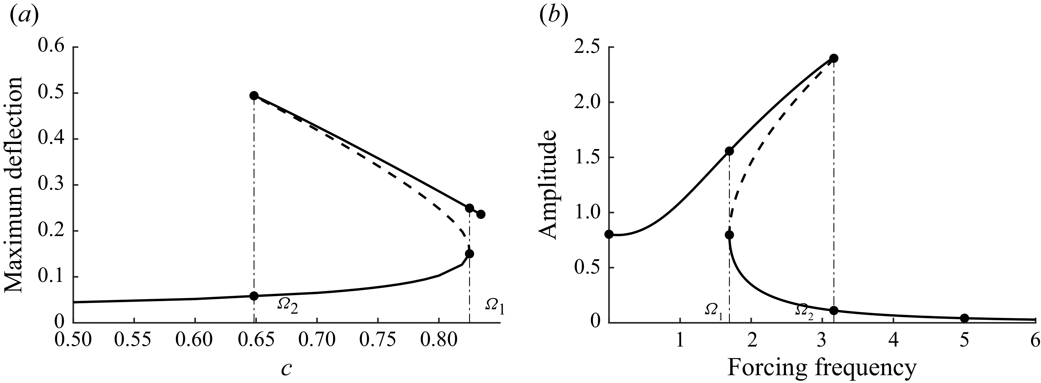
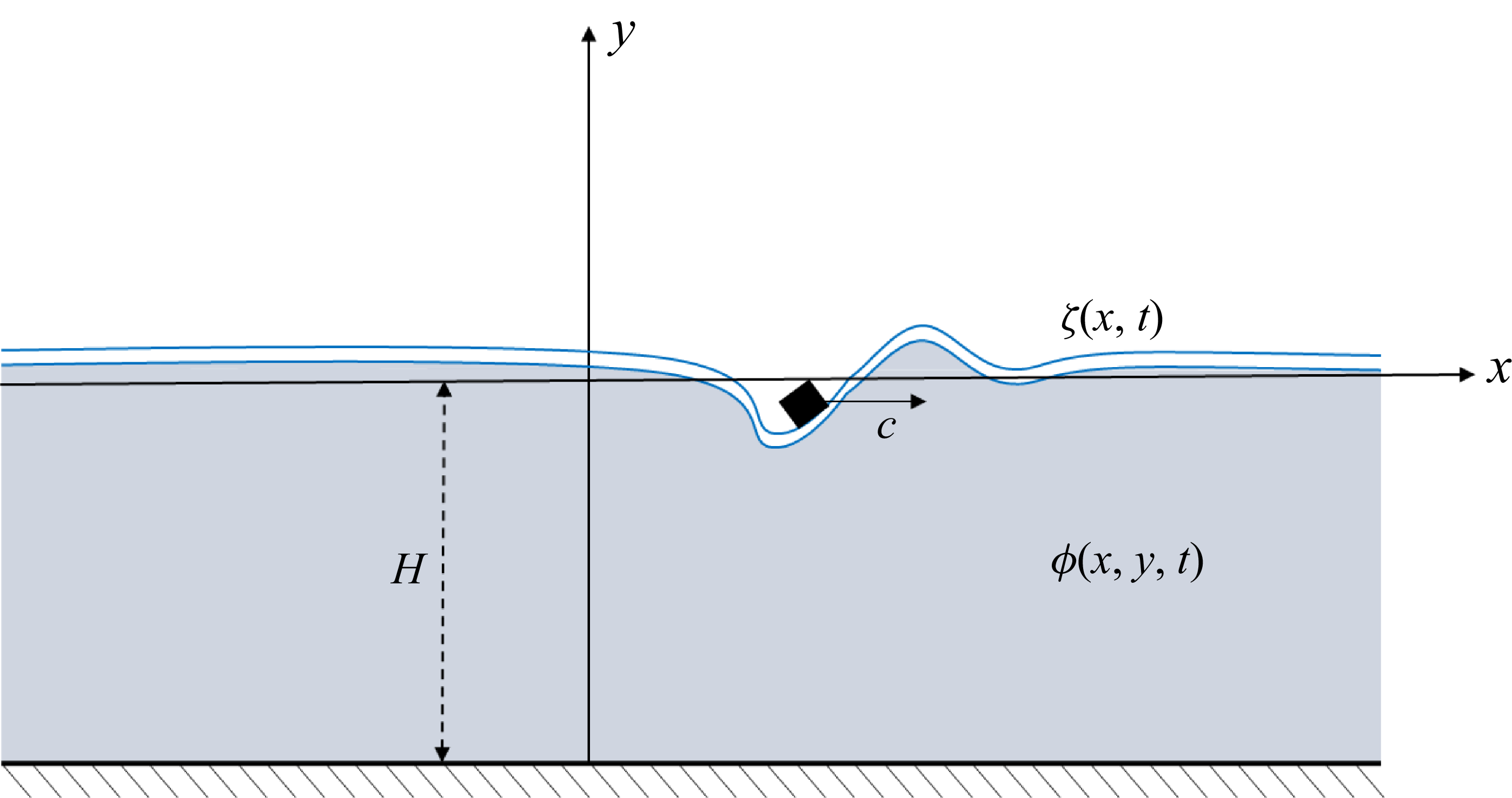

 μ=0.2
 H=1
 P=0.1
 N=1024
 a
 max|ζ|
 c
 c1
 c2
 μ=0
 μ=0.2
 P=0.1
 b−d
 ζ(x)
 c=0.75
 b
 c
 d
 b
 c
 d

 a
 Re(λ)
 Re(λ)≈0.02
 b
 c=0.75
 q1(ξ)

 c=0.75
 a
 b
 c
 θ(0)=0.99θ0
 θ(0)=1.01θ0
 θ0
 d
 μ=0.2
 H=1
 P=0.1
 N=1024
 Δt=10−3
 tfinal=1000

 a,c
 ζ(x,t)
 x=0
 b,d
 (c,max|ζ|)
 a,b
 c1
 c1
 c,d
 c2
 c>c2
 c2
 d
 c2

 μ
 P0
 a
 c1
 c2
 b
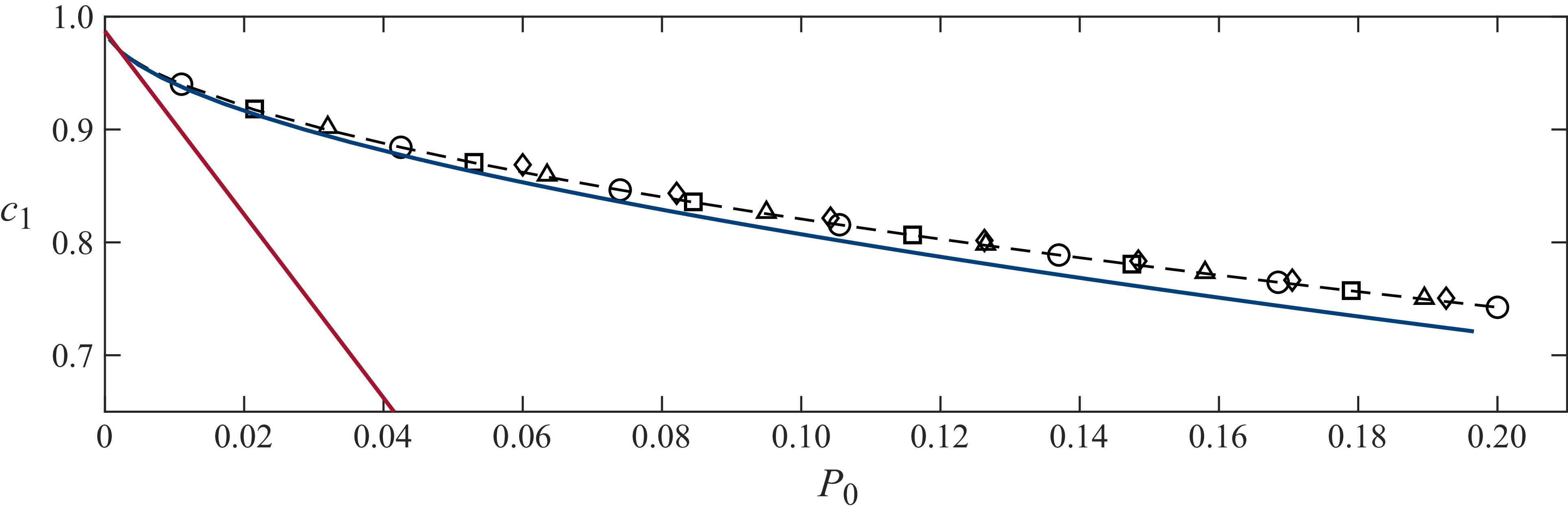
 c1
 P0
 H=1
 c1(u)
 μ=0
 μ=0.01
 μ=0.05
 μ=0.10
 μ=0.20
 P0→0
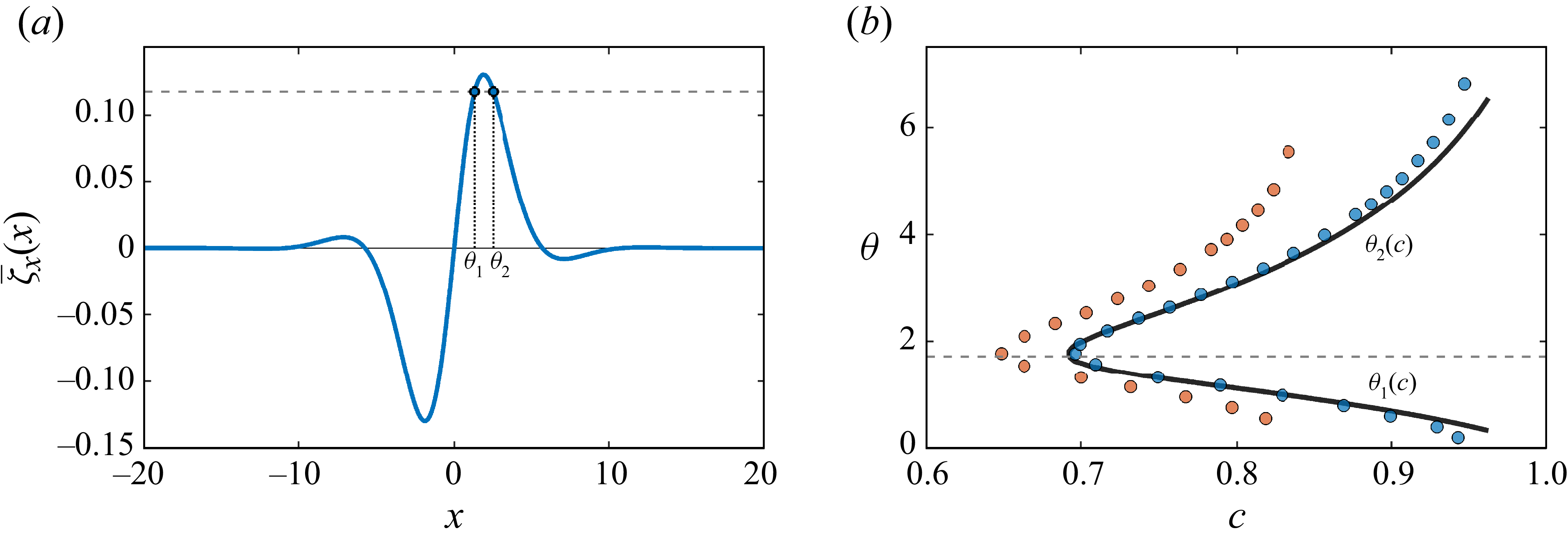
 a
 μ/P0=2
 c=0.75
 ζ¯x
 c(μ/P0)∫ζ¯x2dx
 θ1
 θ2
 θ
 c
 μ=0.2
 P0=0.1
 μ=0.02
 P0=0.01
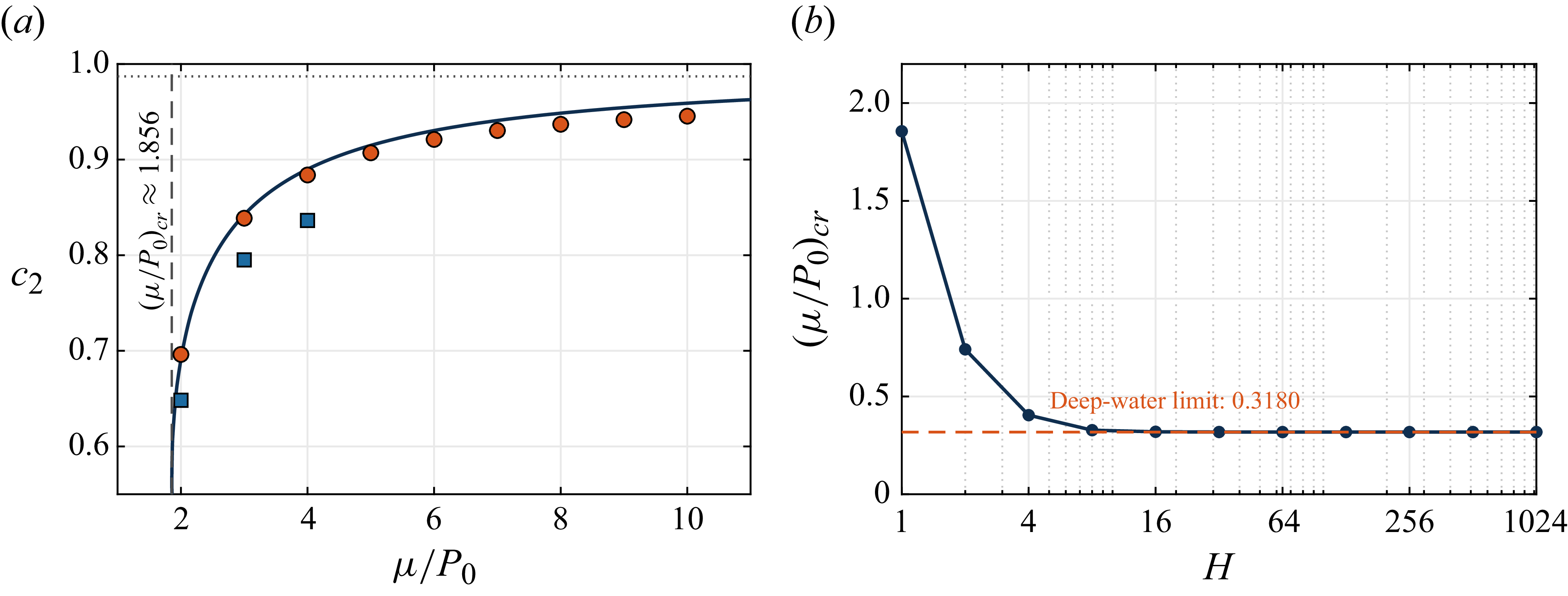
 a
 c2(0)
 μ/P0
 H=1
 P0=0.1
 P0=0.01
 (μ/P0)cr≈1.856
 b
 (μ/P0)cr
 H
 (μ/P0)cr≈0.3180

 a
 max|ζ|
 c
 y=0
 y=1
 b
 Re(λ)
 Re(λ)=0
 μ=0.2
 H=1
 P0=0.1

 H=1
 (θ,a)
 a
 c
 b
 c2
 c
 c>c1
 b

 a
 c≈0.77
 b
 ζ(x)
 a
 c
 μ=0
 c=0.81
 d
 μ=0.2
 P0=0.1
 b−d
 a
 b
 c
 d


