1 Introduction
Primary double-diffusive instabilities, which include fingering and diffusive convection, are caused by unequal molecular diffusivities of individual density components (Stern Reference Stern1960). In the oceanographic context, the two major density constituents of seawater are the temperature (
 $T$
) and salinity (
 $S$
), with the temperature diffusivity exceeding that of salinity by two orders of magnitude. Given such a disparity in molecular diffusivities, it is perhaps not surprising that, under favourable conditions, double-diffusive processes can be highly vigorous and actively influence the water mass composition of the World Ocean (e.g. Schmitt Reference Schmitt1994; Radko Reference Radko2013). The main subject of the present discussion is fingering convection, which occurs when both temperature and salinity decrease with depth. The primary double-diffusive instability in this regime is realized in the form of narrow (a few centimetres wide) vertically elongated filaments known as salt fingers. However, an even more intriguing and dynamically significant consequence of double diffusion is the spontaneous emergence of secondary coherent structures, operating on spatial and temporal scales significantly exceeding those of primary instability. These phenomena include intrusions (Stern Reference Stern1967), collective instability waves (Stern Reference Stern1969) and thermohaline staircases (Stern & Turner Reference Stern and Turner1969). The term ‘staircase’ in this context describes stacks of homogeneous layers separated by sharp interfaces, frequently seen in vertical
 $T{-}S$
profiles from ocean regions particularly susceptible to double-diffusive convection (e.g. Zodiatis & Gasparini Reference Zodiatis and Gasparini1996; Schmitt et al.
Reference Schmitt, Ledwell, Montgomery, Polzin and Toole2005; Bryden et al.
Reference Bryden, Schroeder, Sparnocchia, Borghini and Vetrano2014).
The most common approach to the analysis of secondary double-diffusive phenomena is based on the application of the flux-gradient laws (e.g. Stern, Radko & Simeonov Reference Stern, Radko and Simeonov2001; Stern & Simeonov Reference Stern and Simeonov2002; Traxler et al.
Reference Traxler, Stellmach, Garaud, Radko and Brummel2011). These laws, which are inspired by Fick’s diffusion model, postulate that the microstructure-driven fluxes of temperature and salinity
 $(F_{T},F_{S})$
are proportional to the corresponding large-scale gradients
 $(\unicode[STIX]{x2202}T_{ls}/\unicode[STIX]{x2202}z,\unicode[STIX]{x2202}S_{ls}/\unicode[STIX]{x2202}z)$
:
 $$\begin{eqnarray}\left.\begin{array}{@{}c@{}}\displaystyle F_{T}=-K_{T}\frac{\unicode[STIX]{x2202}T_{ls}}{\unicode[STIX]{x2202}z},\\ \displaystyle F_{S}=-K_{S}\frac{\unicode[STIX]{x2202}S_{ls}}{\unicode[STIX]{x2202}z}.\end{array}\right\}\end{eqnarray}$$
The significance of flux-gradient laws for the advancement of double-diffusive convection theory is hard to overstate. These laws are the bedrock for models of thermohaline interleaving (Stern Reference Stern1967; Merryfield Reference Merryfield2000; Ruddick & Kerr Reference Ruddick and Kerr2003; Mueller, Smyth & Ruddick Reference Mueller, Smyth and Ruddick2007; Smyth & Ruddick Reference Smyth and Ruddick2010), collective instability waves (Stern et al. Reference Stern, Radko and Simeonov2001; Stern & Simeonov Reference Stern and Simeonov2002; Radko & Stern Reference Radko and Stern2011) and thermohaline layering (Radko Reference Radko2003; Stellmach et al. Reference Stellmach, Traxler, Garaud, Brummell and Radko2011). It should also be mentioned that double-diffusive models of this nature are not restricted to ocean science. Parallel developments have been reported, for instance, in the astrophysical context, as recently reviewed by Garaud (Reference Garaud2018).
Nevertheless, it should be realized that flux-gradient laws are not universally applicable. For instance, these laws are known to fail when the size of the phenomenon of interest is comparable to the scale of microstructure which those laws strive to parametrize. A recent study (Radko Reference Radko2014) attempted to identify the range of scales adequately represented by fingering flux-gradient laws. This investigation has led to an estimate of the critical point-of-failure scale (
 $H_{pof}$
) below which the flux-gradient model becomes suspect. It was shown that
 $H_{pof}$
can be surprisingly large – approximately 3 m for representative oceanic conditions – exceeding the molecular heat dissipation scale by at least two orders of magnitude.
Unfortunately, the consequences of the failure of flux-gradient laws at small scales (
 $H\lesssim H_{pof}$
) are not limited to benign quantitative errors. More ominous and fundamental complications arise, for example, in models of thermohaline staircases (Radko Reference Radko2003, Reference Radko2014; Stellmach et al.
Reference Stellmach, Traxler, Garaud, Brummell and Radko2011). In these studies, linear analysis of the flux-gradient laws reveals the existence of unstable horizontally uniform modes. Numerical simulations confirm their existence and, furthermore, demonstrate that these modes ultimately transform the initially uniform background gradient into a series of well-mixed layers – structures that are highly suggestive of oceanic staircases. However, the analytical flux-gradient model erroneously predicts that the growth rate of layering modes monotonically increases without bound with the vertical wavenumber. Besides being unphysical, this result is inconsistent with direct numerical simulations (DNS), which show that the wavelength of the fastest-growing layering mode exceeds the salt-finger scale by more than an order of magnitude (e.g. Radko Reference Radko2014). The ultraviolet catastrophe of analytical solutions, apparently an artifact of indiscriminate application of the flux-gradient laws to all scales, precludes theoretical analyses of such basic properties of layering instability as its preferred wavelength or the maximal growth rate.
It should be noted that it is not uncommon for the ultraviolet catastrophe to arise in theoretical models of turbulent systems, and several attempts have been made to alleviate its consequences. For instance, the simple remedy for the unphysical behaviour of the flux-gradient laws employed in our previous investigations (Radko Reference Radko2005, Reference Radko2014; Radko et al. Reference Radko, Flanagan, Stellmach and Timmermans2014) was the inclusion of scale-selective damping terms, which stabilize short wavelengths and thereby eliminate the ultraviolet catastrophe. Paparella & von Hardenberg (Reference Paparella and von Hardenberg2012) argue that the ultraviolet catastrophe is caused by up-gradient buoyancy fluxes driven by primary fingering instabilities. These fluxes are countered at smaller scales by down-gradient mixing associated with secondary fingering instabilities, which can be parametrized accordingly (Paparella & von Hardenberg Reference Paparella and von Hardenberg2014). The model of layering in stratified one-component flows (Balmforth, Llewellyn Smith & Young Reference Balmforth, Llewellyn Smith and Young1998b ) incorporates the delayed response of the vertical fluxes to changes in stratification, which ultimately stabilizes modes with small wavelength.
The aforementioned models adopt an inherently heuristic approach to the problem of failure of flux-gradient laws, which is based on the identification of potentially significant stabilizing small-scale processes and their inclusion in the model formulation. The resulting modifications, which are introduced on a case-by-case basis, serve their immediate purpose by making the corresponding large-scale models well-posed. However, the question arises whether a sufficiently generic algorithm can be designed to resolve the problem of the ultraviolet catastrophe for a wide class of problems and concurrently reduce arbitrariness in the selection of relevant stabilizing models. The present study meets this challenge by developing fingering flux laws using techniques of multiscale analysis. Multiscale modelling is a broad and vibrant field with numerous applications in various physical sciences, as discussed, for example, in the review by Mei & Vernescu (Reference Mei and Vernescu2010). Multiscale mechanics is based directly on governing equations and it is, therefore, free of the empirical parametrizations required by other analytical models of turbulent transport. Its methods generally assume an analytical small-scale pattern and analyse its interaction with large-scale flows, which ultimately leads to explicit evolutionary large-scale equations. The analyses are based on the asymptotic expansion in powers of a small parameter (
 $\unicode[STIX]{x1D700}$
), which represents the ratio of typical scales of the primary pattern (salt fingers in our case) and those of larger structures (layering modes in the present study). Multiscale models can be viewed as a mechanistic alternative to statistical theories of turbulence (e.g. Krommes & Kim Reference Krommes and Kim2000; Farrell & Ioannou Reference Farrell and Ioannou2007; Tobias, Dagon & Marston Reference Tobias, Dagon and Marston2011) exemplified by studies of the spontaneous generation and maintenance of large-scale jets in barotropic eddying flows (e.g. Marston, Conover & Schneider Reference Marston, Conover and Schneider2008; Srinivasan & Young Reference Srinivasan and Young2012).
The simplest primary pattern used in multiscale mechanics is the Kolmogorov model, represented by a parallel shear flow with sinusoidal velocity profile (e.g. Meshalkin & Sinai Reference Meshalkin and Sinai1961; Manfroi & Young Reference Manfroi and Young1999, Reference Manfroi and Young2002; Balmforth & Young Reference Balmforth and Young2002, Reference Balmforth and Young2005; Radko Reference Radko2014). However, multiscale methods have been generalized to include more complicated two-dimensional patterns, including cellular, hexagonal or dipolar structures (e.g. Gama, Vergassola & Frisch Reference Gama, Vergassola and Frisch1994; Vanneste Reference Vanneste2000; Novikov & Papanicolaou Reference Novikov and Papanicolaou2001; Radko Reference Radko2011). Although less common, multiscale models based on three-dimensional small-scale patterns have also been developed (Dubrulle & Frisch Reference Dubrulle and Frisch1991; Wirth et al. Reference Wirth, Gama and Frisch1995).
Perhaps the most significant limitation of conventional multiscale models is the sensitive dependence of the obtained large-scale solutions on the assumed small-scale patterns (e.g. Gama et al. Reference Gama, Vergassola and Frisch1994; Novikov & Papanicolaou Reference Novikov and Papanicolaou2001; Radko Reference Radko2011). For configurations in which small-scale fields are disorganized and time-dependent, as in the present study, this sensitivity presents a major obstacle for the quantitative representation of cross-scale interactions. To surmount this complication, a proposition has recently been made (Radko Reference Radko2016a ) to construct small-scale patterns for multiscale modelling using realistic, dynamically consistent flow fields – an approach that was referred to as the average eddy model. Such small-scale structures can be readily extracted from numerical simulations, and the resulting multiscale solutions offer a transparent and unambiguous description of the interaction between microstructure and large-scale stratification. In the present study, this version of the multiscale model is employed to formulate generalized flux laws, which take into account non-uniformities of the background stratification. These laws are then used to investigate the dynamics of thermohaline layering.
An important feature of the present implementation of the multiscale method is that the expansion is carried out beyond the leading order in the separation parameter
 $\unicode[STIX]{x1D700}$
. We demonstrate that truncating the asymptotic series at the leading order is equivalent to adopting the flux-gradient model with all its deficiencies. However, extending the expansion to the next order in
 $\unicode[STIX]{x1D700}$
makes it possible to take into account non-uniformities of the background stratification. While the proposed model still assumes scale separation between fingers and layering modes (
 $\unicode[STIX]{x1D700}\ll 1$
), its performance dramatically improves with the addition of higher-order components. In particular, this generalization is shown to alleviate complications associated with the failure of the flux-gradient model at small scales, most notably eliminating its ultraviolet catastrophe. It should also be emphasized that, aside from the pragmatic task of parametrizing salt fingers, the dynamics of double-diffusive convection in non-uniform gradients is of interest in its own right (e.g. Balmforth, Casti & Julien Reference Balmforth, Casti and Julien1998a
). The present investigation attempts to concurrently address both aspects of the problem.
This paper is organized as follows. In § 2, we describe the model configuration and present illustrative numerical examples of thermohaline layering. The multiscale theory of layering is formulated in § 3. In § 4, we examine linear large-scale solutions derived using the multiscale model and compare them with their flux-gradient counterparts. The parametric staircase model, which is based on the generalized flux laws, is presented in § 5. In § 6, we draw conclusions and summarize our findings.
2 Formulation
In order to describe spontaneous layering in a doubly stratified fluid, the total temperature and salinity fields
 $(T_{tot}^{\ast },S_{tot}^{\ast })$
are separated into the background state
 $(\bar{\bar{T}}^{\ast },\bar{\bar{S}}^{\ast })$
, representing uniform vertical gradients, and a departure
 $(T^{\ast },S^{\ast })$
from them:
 $$\begin{eqnarray}\left.\begin{array}{@{}c@{}}T_{tot}^{\ast }=\bar{\bar{T}}^{\ast }+T^{\ast }=A_{T}z^{\ast }+A_{T0}+T^{\ast },\\ S_{tot}^{\ast }=\bar{\bar{S}}^{\ast }+S^{\ast }=A_{S}z^{\ast }+A_{S0}+S^{\ast },\end{array}\right\}\end{eqnarray}$$
where
 $(A_{T},A_{T0},A_{S},A_{S0})$
are constants and the asterisks denote dimensional field variables. Our focus is on the finger-favourable stratification (
 $(\unicode[STIX]{x2202}\bar{\bar{T}}^{\ast }/\unicode[STIX]{x2202}z^{\ast })=A_{T}>0$
,
 $(\unicode[STIX]{x2202}\bar{\bar{S}}^{\ast }/\unicode[STIX]{x2202}z^{\ast })=A_{S}>0$
). In the present version of the theory, we ignore planetary rotation, compressibility and the nonlinearity of the equation of state, and express the governing Boussinesq equations of motion in terms of perturbations
 $(T^{\ast },S^{\ast })$
:
 $$\begin{eqnarray}\left.\begin{array}{@{}c@{}}\displaystyle \frac{\unicode[STIX]{x2202}T^{\ast }}{\unicode[STIX]{x2202}t^{\ast }}+\boldsymbol{v}^{\ast }\boldsymbol{\cdot }\unicode[STIX]{x1D735}T^{\ast }+w^{\ast }\frac{\unicode[STIX]{x2202}\bar{\bar{T}}^{\ast }}{\unicode[STIX]{x2202}z^{\ast }}=k_{T}\unicode[STIX]{x1D6FB}^{2}T^{\ast },\\ \displaystyle \frac{\unicode[STIX]{x2202}S^{\ast }}{\unicode[STIX]{x2202}t^{\ast }}+\boldsymbol{v}^{\ast }\boldsymbol{\cdot }\unicode[STIX]{x1D735}S^{\ast }+w^{\ast }\frac{\unicode[STIX]{x2202}\bar{\bar{S}}^{\ast }}{\unicode[STIX]{x2202}z^{\ast }}=k_{S}\unicode[STIX]{x1D6FB}^{2}S^{\ast },\\ \displaystyle \frac{\unicode[STIX]{x2202}\boldsymbol{v}^{\ast }}{\unicode[STIX]{x2202}t^{\ast }}+\boldsymbol{v}^{\ast }\boldsymbol{\cdot }\unicode[STIX]{x1D735}\boldsymbol{v}^{\ast }=-\frac{1}{\unicode[STIX]{x1D70C}_{0}^{\ast }}\unicode[STIX]{x1D735}p^{\ast }+g(\unicode[STIX]{x1D6FC}T^{\ast }-\unicode[STIX]{x1D6FD}S^{\ast })\boldsymbol{k}+\unicode[STIX]{x1D708}\unicode[STIX]{x1D6FB}^{2}\boldsymbol{v}^{\ast },\\ \displaystyle \unicode[STIX]{x1D735}\boldsymbol{\cdot }\boldsymbol{v}^{\ast }=0,\end{array}\right\}\end{eqnarray}$$
where
 $\boldsymbol{v}^{\ast }=(u^{\ast },v^{\ast },w^{\ast })$
is the velocity,
 $\boldsymbol{k}$
is the vertical unit vector,
 $p^{\ast }$
is the dynamic pressure,
 $g$
is gravity,
 $(\unicode[STIX]{x1D6FC},\unicode[STIX]{x1D6FD})$
are the thermal expansion and haline contraction coefficients,
 $(k_{T},k_{S})$
are the molecular diffusivities of heat and salt, and
 $\unicode[STIX]{x1D70C}_{0}^{\ast }$
is the reference density.
To reduce the number of controlling parameters, system (2.2) is non-dimensionalized using
 $l=[k_{T}\unicode[STIX]{x1D708}/(g\unicode[STIX]{x1D6FC}\,\unicode[STIX]{x2202}\bar{\bar{T}}^{\ast }/\unicode[STIX]{x2202}z^{\ast })]^{1/4}$
,
 $k_{T}/l$
,
 $l^{2}/k_{T}$
and
 $\unicode[STIX]{x1D70C}_{0}^{\ast }\unicode[STIX]{x1D708}k_{T}/l^{2}$
as the units of length, velocity, time and pressure, respectively. These scales reflect characteristics of individual salt fingers, and therefore the resulting non-dimensional system is most appropriate for the analysis of microscale dynamics of double-diffusive convection (e.g. Radko Reference Radko2013). The expansion/contraction coefficients
 $(\unicode[STIX]{x1D6FC},\unicode[STIX]{x1D6FD})$
are incorporated in
 $(T^{\ast },S^{\ast })$
, and
 $\unicode[STIX]{x1D6FC}(\unicode[STIX]{x2202}\bar{\bar{T}}^{\ast }/\unicode[STIX]{x2202}z^{\ast })l$
is used as the scale for both temperature and salinity perturbations:
 $$\begin{eqnarray}\unicode[STIX]{x1D6FC}T^{\ast }\rightarrow \unicode[STIX]{x1D6FC}\frac{\unicode[STIX]{x2202}\bar{\bar{T}}^{\ast }}{\unicode[STIX]{x2202}z^{\ast }}lT,\quad \unicode[STIX]{x1D6FD}S^{\ast }\rightarrow \unicode[STIX]{x1D6FC}\frac{\unicode[STIX]{x2202}\bar{\bar{T}}^{\ast }}{\unicode[STIX]{x2202}z^{\ast }}lS.\end{eqnarray}$$
After non-dimensionalization, the governing equations (2.2) reduce to
 $$\begin{eqnarray}\left.\begin{array}{@{}c@{}}\displaystyle \frac{\unicode[STIX]{x2202}T}{\unicode[STIX]{x2202}t}+\boldsymbol{v}\boldsymbol{\cdot }\unicode[STIX]{x1D735}T+w=\unicode[STIX]{x1D6FB}^{2}T,\\ \displaystyle \frac{\unicode[STIX]{x2202}S}{\unicode[STIX]{x2202}t}+\boldsymbol{v}\boldsymbol{\cdot }\unicode[STIX]{x1D735}S+\frac{w}{\bar{\bar{R}}_{\unicode[STIX]{x1D70C}}}=\unicode[STIX]{x1D70F}\unicode[STIX]{x1D6FB}^{2}S,\\ \displaystyle \frac{1}{Pr}\left(\frac{\unicode[STIX]{x2202}}{\unicode[STIX]{x2202}t}\boldsymbol{v}+\boldsymbol{v}\boldsymbol{\cdot }\unicode[STIX]{x1D735}\boldsymbol{v}\right)=-\unicode[STIX]{x1D735}p+(T-S)\boldsymbol{k}+\unicode[STIX]{x1D6FB}^{2}\boldsymbol{v},\\ \unicode[STIX]{x1D735}\boldsymbol{\cdot }\boldsymbol{v}=0,\end{array}\right\}\end{eqnarray}$$
where
 $\bar{\bar{R}}_{\unicode[STIX]{x1D70C}}=[\unicode[STIX]{x1D6FC}(\unicode[STIX]{x2202}\bar{\bar{T}}^{\ast }/\unicode[STIX]{x2202}z^{\ast })]/[\unicode[STIX]{x1D6FD}(\unicode[STIX]{x2202}\bar{\bar{S}}^{\ast }/\unicode[STIX]{x2202}z^{\ast })]$
is the background density ratio,
 $\unicode[STIX]{x1D70F}=k_{S}/k_{T}$
is the diffusivity ratio and
 $Pr=\unicode[STIX]{x1D708}/k_{T}$
is the Prandtl number. The specific calculations in this study are based on the two-dimensional (
 $x,z$
) version of the Boussinesq system (2.4):
 $$\begin{eqnarray}\left.\begin{array}{@{}c@{}}\displaystyle \frac{\unicode[STIX]{x2202}T}{\unicode[STIX]{x2202}t}+J(\unicode[STIX]{x1D713},T)+\frac{\unicode[STIX]{x2202}\unicode[STIX]{x1D713}}{\unicode[STIX]{x2202}x}=\unicode[STIX]{x1D6FB}^{2}T,\\ \displaystyle \frac{\unicode[STIX]{x2202}S}{\unicode[STIX]{x2202}t}+J(\unicode[STIX]{x1D713},S)+\frac{1}{\bar{\bar{R}}_{\unicode[STIX]{x1D70C}}}\frac{\unicode[STIX]{x2202}\unicode[STIX]{x1D713}}{\unicode[STIX]{x2202}x}=\unicode[STIX]{x1D70F}\unicode[STIX]{x1D6FB}^{2}S,\\ \displaystyle \frac{\unicode[STIX]{x2202}}{\unicode[STIX]{x2202}t}\unicode[STIX]{x1D6FB}^{2}\unicode[STIX]{x1D713}+J(\unicode[STIX]{x1D713},\unicode[STIX]{x1D6FB}^{2}\unicode[STIX]{x1D713})=Pr\left[\frac{\unicode[STIX]{x2202}}{\unicode[STIX]{x2202}x}(T-S)+\unicode[STIX]{x1D6FB}^{4}\unicode[STIX]{x1D713}\right],\end{array}\right\}\end{eqnarray}$$
where
 $\unicode[STIX]{x1D713}$
is the streamfunction, such that
 $(u,w)=(-\unicode[STIX]{x2202}\unicode[STIX]{x1D713}/\unicode[STIX]{x2202}z,\unicode[STIX]{x2202}\unicode[STIX]{x1D713}/\unicode[STIX]{x2202}x)$
and
 $J(a,b)\equiv (\unicode[STIX]{x2202}a/\unicode[STIX]{x2202}x)(\unicode[STIX]{x2202}b/\unicode[STIX]{x2202}z)-(\unicode[STIX]{x2202}a/\unicode[STIX]{x2202}z)(\unicode[STIX]{x2202}b/\unicode[STIX]{x2202}x)$
is the Jacobian. Two-dimensional simulations carry an obvious benefit of numerical efficiency, which affords a more comprehensive exploration of the parameter space. It should also be noted that externally induced large-scale flows (e.g. internal waves), which are ubiquitous in the ocean, favour formation of salt sheets aligned in the direction of the background shear (Linden Reference Linden1974; Kimura & Smyth Reference Kimura and Smyth2007; Radko et al.
Reference Radko, Ball, Colosi and Flanagan2015). In such cases, salt-finger dynamics becomes effectively two-dimensional, which implies that analyses based on model (2.5) are more oceanographically relevant.
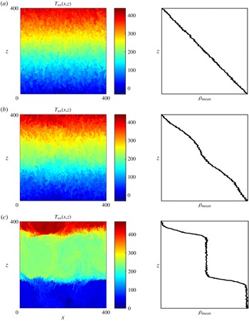
To briefly describe the key features of fully developed fingering convection, we present (figure 1) a typical numerical simulation. The two-dimensional model (2.5) was integrated in time using the dealiased pseudospectral method (e.g. Stern et al.
Reference Stern, Radko and Simeonov2001; Stellmach et al.
Reference Stellmach, Traxler, Garaud, Brummell and Radko2011) with periodic boundary conditions applied to the streamfunction
 $\unicode[STIX]{x1D713}$
and to the perturbation temperature and salinity fields
 $(T,S)$
in each spatial direction. The governing non-dimensional parameters for this experiment are
 $(R_{\unicode[STIX]{x1D70C}},Pr,\unicode[STIX]{x1D70F})=(1.5,7,0.01)$
. The domain size is
 $400\times 400$
, which corresponds to
 $4~\text{m}\times 4~\text{m}$
for representative oceanographic scales, and the numerical mesh contains
 $(N_{x},N_{z})=(6144,6144)$
grid points. The evolution of the temperature field
 $T(x,y)$
from the initial state represented by a random low-amplitude distribution of
 $(T,S,\unicode[STIX]{x1D713})$
is shown in figure 1(a–c). The first stage is characterized by the development of primary fingering instabilities (figure 1
a), which is followed by the spontaneous emergence of a relatively large-scale horizontally uniform mode (figure 1
b). This mode monotonically grows in time, eventually producing two well-defined mixed layers separated by thin high-gradient interfaces (figure 1
c). Note that the wavelength of the amplifying mode in figure 1 (
 $L=200$
) exceeds the scale of individual fingers (
 $L\sim 10$
) by more than an order of magnitude. The selection of the preferred wavelength of layering modes remains one of the most intriguing and fundamental unresolved problems in the theory of double-diffusive convection. The flux-gradient model (Radko Reference Radko2003) does not provide definitive answers in this regard, erroneously predicting that the growth rate of layering modes monotonically increases with wavenumber, motivating the following alternative approach.
Two-dimensional DNS for
 $(R_{\unicode[STIX]{x1D70C}},\unicode[STIX]{x1D70F},Pr)=(1.5,0.01,7)$
. The instantaneous temperature fields (left panels) and horizontally averaged density profiles (right panels) are shown for (a)
 $t=100$
, (b)
 $t=1450$
and (c)
 $t=2040$
. Note the gradual amplification of the large-scale mode and the transition of the system to a well-defined layered configuration.

3 Layering instability as a multiscale problem
The intent of this section is to explain the properties of large-scale patterns (e.g. figure 1), which spontaneously emerge from initially homogeneous fingering fields using techniques of asymptotic multiscale analysis. Theoretical development generally follows Radko (Reference Radko2016a ) and therefore here we present an abbreviated description of the multiscale model.
3.1 Formulation
First, the new large-scale spatial and temporal variables
 $(Z,t_{2},t_{4})$
are introduced, which are related to the original variables as follows:
 $$\begin{eqnarray}Z=\unicode[STIX]{x1D700}z,\quad t_{2}=\unicode[STIX]{x1D700}^{2}t,\quad t_{4}=\unicode[STIX]{x1D700}^{4}t,\end{eqnarray}$$
where
 $\unicode[STIX]{x1D700}$
is the expansion parameter representing the difference in spatial scales of primary (fingering) and secondary (layering) instabilities. The derivatives in the governing system (2.5) are replaced accordingly:
 $$\begin{eqnarray}\frac{\unicode[STIX]{x2202}}{\unicode[STIX]{x2202}t}\rightarrow \frac{\unicode[STIX]{x2202}}{\unicode[STIX]{x2202}t}+\unicode[STIX]{x1D700}^{2}\frac{\unicode[STIX]{x2202}}{\unicode[STIX]{x2202}t_{2}}+\unicode[STIX]{x1D700}^{4}\frac{\unicode[STIX]{x2202}}{\unicode[STIX]{x2202}t_{4}},\quad \frac{\unicode[STIX]{x2202}}{\unicode[STIX]{x2202}z}\rightarrow \frac{\unicode[STIX]{x2202}}{\unicode[STIX]{x2202}z}+\unicode[STIX]{x1D700}\frac{\unicode[STIX]{x2202}}{\unicode[STIX]{x2202}Z}.\end{eqnarray}$$
We treat
 $(x,z,t,Z,t_{2},t_{4})$
as independent variables and replace the
 $z$
- and
 $t$
-derivatives in governing equations (2.5) using transformation (3.2), which results in
 $$\begin{eqnarray}\left.\begin{array}{@{}l@{}}\displaystyle \frac{\unicode[STIX]{x2202}T}{\unicode[STIX]{x2202}t}+\unicode[STIX]{x1D700}^{2}\frac{\unicode[STIX]{x2202}T}{\unicode[STIX]{x2202}t_{2}}+\unicode[STIX]{x1D700}^{4}\frac{\unicode[STIX]{x2202}T}{\unicode[STIX]{x2202}t_{4}}+J_{xz}(\unicode[STIX]{x1D713},T)+\unicode[STIX]{x1D700}J_{xZ}(\unicode[STIX]{x1D713},T)+\frac{\unicode[STIX]{x2202}\unicode[STIX]{x1D713}}{\unicode[STIX]{x2202}x}\\ \displaystyle \qquad =\left(\unicode[STIX]{x1D6FB}^{2}+2\unicode[STIX]{x1D700}\frac{\unicode[STIX]{x2202}^{2}}{\unicode[STIX]{x2202}z\unicode[STIX]{x2202}Z}+\unicode[STIX]{x1D700}^{2}\frac{\unicode[STIX]{x2202}^{2}}{\unicode[STIX]{x2202}Z^{2}}\right)T,\\ \displaystyle \frac{\unicode[STIX]{x2202}S}{\unicode[STIX]{x2202}t}+\unicode[STIX]{x1D700}^{2}\frac{\unicode[STIX]{x2202}S}{\unicode[STIX]{x2202}t_{2}}+\unicode[STIX]{x1D700}^{4}\frac{\unicode[STIX]{x2202}S}{\unicode[STIX]{x2202}t_{4}}+J_{xz}(\unicode[STIX]{x1D713},S)+\unicode[STIX]{x1D700}J_{xZ}(\unicode[STIX]{x1D713},S)+\frac{1}{\bar{\bar{R}}_{\unicode[STIX]{x1D70C}}}\frac{\unicode[STIX]{x2202}\unicode[STIX]{x1D713}}{\unicode[STIX]{x2202}x}\\ \displaystyle \qquad =\unicode[STIX]{x1D70F}\left(\unicode[STIX]{x1D6FB}^{2}+2\unicode[STIX]{x1D700}\frac{\unicode[STIX]{x2202}^{2}}{\unicode[STIX]{x2202}z\unicode[STIX]{x2202}Z}+\unicode[STIX]{x1D700}^{2}\frac{\unicode[STIX]{x2202}^{2}}{\unicode[STIX]{x2202}Z^{2}}\right)S,\\ \displaystyle \frac{\unicode[STIX]{x2202}}{\unicode[STIX]{x2202}t}\unicode[STIX]{x1D70D}+\unicode[STIX]{x1D700}^{2}\frac{\unicode[STIX]{x2202}\unicode[STIX]{x1D70D}}{\unicode[STIX]{x2202}t_{2}}+\unicode[STIX]{x1D700}^{4}\frac{\unicode[STIX]{x2202}\unicode[STIX]{x1D70D}}{\unicode[STIX]{x2202}t_{4}}+J_{xz}(\unicode[STIX]{x1D713},\unicode[STIX]{x1D70D})+\unicode[STIX]{x1D700}J_{xZ}(\unicode[STIX]{x1D713},\unicode[STIX]{x1D70D})\\ \displaystyle \qquad =Pr\left[\frac{\unicode[STIX]{x2202}}{\unicode[STIX]{x2202}x}(T-S)+\left(\unicode[STIX]{x1D6FB}^{2}+2\unicode[STIX]{x1D700}\frac{\unicode[STIX]{x2202}^{2}}{\unicode[STIX]{x2202}z\unicode[STIX]{x2202}Z}+\unicode[STIX]{x1D700}^{2}\frac{\unicode[STIX]{x2202}^{2}}{\unicode[STIX]{x2202}Z^{2}}\right)\unicode[STIX]{x1D70D}\right],\\ \displaystyle \unicode[STIX]{x1D70D}=\left(\unicode[STIX]{x1D6FB}^{2}+2\unicode[STIX]{x1D700}\frac{\unicode[STIX]{x2202}^{2}}{\unicode[STIX]{x2202}\displaystyle z\unicode[STIX]{x2202}Z}+\unicode[STIX]{x1D700}^{2}\frac{\unicode[STIX]{x2202}^{2}}{\unicode[STIX]{x2202}Z^{2}}\right)\unicode[STIX]{x1D713},\end{array}\right\}\end{eqnarray}$$
where
 $J_{xz}(a,b)\equiv (\unicode[STIX]{x2202}a/\unicode[STIX]{x2202}x)(\unicode[STIX]{x2202}b/\unicode[STIX]{x2202}z)-(\unicode[STIX]{x2202}b/\unicode[STIX]{x2202}x)(\unicode[STIX]{x2202}a/\unicode[STIX]{x2202}z)$
and
 $J_{xZ}(a,b)\equiv (\unicode[STIX]{x2202}a/\unicode[STIX]{x2202}x)(\unicode[STIX]{x2202}b/\unicode[STIX]{x2202}Z)-(\unicode[STIX]{x2202}b/\unicode[STIX]{x2202}x)(\unicode[STIX]{x2202}a/\unicode[STIX]{x2202}Z)$
.
The basic state in the following model is represented by the fully developed and statistically homogeneous fingering field, which varies only on small scales:
 $$\begin{eqnarray}\left.\begin{array}{@{}c@{}}\bar{T}=\bar{T}(x,z,t),\\ \bar{S}=\bar{S}(x,z,t),\\ \bar{\unicode[STIX]{x1D713}}=\bar{\unicode[STIX]{x1D713}}(x,z,t).\end{array}\right\}\end{eqnarray}$$
To examine the interaction of the basic field (3.4) with large scales, it is perturbed by long-wavelength horizontally uniform temperature and salinity patterns
 $(T_{0},S_{0})$
. The solution is sought in terms of a series in
 $\unicode[STIX]{x1D700}\ll 1$
:
 $$\begin{eqnarray}\left.\begin{array}{@{}c@{}}T=\bar{T}(x,z,t)+T_{0}(Z,t_{2},t_{4})+\unicode[STIX]{x1D700}T_{1}(x,z,Z,t,t_{2},t_{4})+\unicode[STIX]{x1D700}^{2}T_{2}(x,z,Z,t,t_{2},t_{4})+\cdots \,,\\ S=\bar{S}(x,z,t)+S_{0}(Z,t_{2},t_{4})+\unicode[STIX]{x1D700}S_{1}(x,z,Z,t,t_{2},t_{4})+\unicode[STIX]{x1D700}^{2}S_{2}(x,z,Z,t,t_{2},t_{4})+\cdots \,,\\ \unicode[STIX]{x1D713}=\bar{\unicode[STIX]{x1D713}}(x,z,t)+\unicode[STIX]{x1D700}\unicode[STIX]{x1D713}_{1}(x,z,Z,t,t_{2},t_{4})+\unicode[STIX]{x1D700}^{2}\unicode[STIX]{x1D713}_{2}(x,z,Z,t,t_{2},t_{4})+\cdots \,.\end{array}\right\}\end{eqnarray}$$
When the expansion (3.5) is substituted into the governing system (3.3) and the terms of the same order are collected, we discover that the individual components
 $(T_{i},S_{i},\unicode[STIX]{x1D713}_{i})$
allow for a solution in the following form:
 $$\begin{eqnarray}\left\{\begin{array}{@{}l@{}}\displaystyle T_{i}=\frac{\unicode[STIX]{x2202}^{i}T_{0}}{\unicode[STIX]{x2202}Z^{i}}\tilde{T}_{iT}(x,z,t)+\frac{\unicode[STIX]{x2202}^{i}S_{0}}{\unicode[STIX]{x2202}Z^{i}}\tilde{T}_{iS}(x,z,t),\\ \displaystyle S_{i}=\frac{\unicode[STIX]{x2202}^{i}T_{0}}{\unicode[STIX]{x2202}Z^{i}}\tilde{S}_{iT}(x,z,t)+\frac{\unicode[STIX]{x2202}^{i}S_{0}}{\unicode[STIX]{x2202}Z^{i}}\tilde{S}_{iS}(x,z,t),\\ \displaystyle \unicode[STIX]{x1D713}_{i}=\frac{\unicode[STIX]{x2202}^{i}T_{0}}{\unicode[STIX]{x2202}Z^{i}}\tilde{\unicode[STIX]{x1D713}}_{iT}(x,z,t)+\frac{\unicode[STIX]{x2202}^{i}S_{0}}{\unicode[STIX]{x2202}Z^{i}}\tilde{\unicode[STIX]{x1D713}}_{iS}(x,z,t),\end{array}\right.\quad i=1,2,\ldots .\end{eqnarray}$$
Thus, each term in the expansion represents a product of a modulating function, which varies on large scales, and the corresponding rapidly varying variable. The latter quantities
 $(\tilde{T}_{iT},\tilde{S}_{iT},\tilde{\unicode[STIX]{x1D713}}_{iT},\tilde{T}_{iS},\tilde{S}_{iS},\tilde{\unicode[STIX]{x1D713}}_{iS})$
are referred to as the auxiliary functions. Note that in (3.6) we included only terms that are linear in
 $(T_{0},S_{0})$
. The linearization was largely motivated by considerations of simplicity and transparency since multiscale models can incorporate large-scale nonlinearities in a relatively straightforward manner (e.g. Gama et al.
Reference Gama, Vergassola and Frisch1994; Novikov & Papanicolaou Reference Novikov and Papanicolaou2001). Furthermore, the linearized model represents a natural starting point for any stability analysis, making it possible to unambiguously determine the growth rates of unstable perturbations. The expansions (3.5) and (3.6) are consistent with governing equations (3.3) as long as the auxiliary functions satisfy partial differential equation (PDE) systems written entirely in terms of small-scale independent variables. For instance, for the first-order (
 $i=1$
) terms, the corresponding auxiliary PDE systems are
 $$\begin{eqnarray}A\left(\begin{array}{@{}c@{}}\tilde{T}_{1T}\\ \tilde{S}_{1T}\\ \tilde{\unicode[STIX]{x1D713}}_{1T}\end{array}\right)=\left(\begin{array}{@{}c@{}}-{\displaystyle \frac{\unicode[STIX]{x2202}\bar{\unicode[STIX]{x1D713}}}{\unicode[STIX]{x2202}x}}\\ 0\\ 0\end{array}\right),\quad A\left(\begin{array}{@{}c@{}}\tilde{T}_{1S}\\ \tilde{S}_{1S}\\ \tilde{\unicode[STIX]{x1D713}}_{1S}\end{array}\right)=\left(\begin{array}{@{}c@{}}0\\ -{\displaystyle \frac{\unicode[STIX]{x2202}\bar{\unicode[STIX]{x1D713}}}{\unicode[STIX]{x2202}x}}\\ 0\end{array}\right),\end{eqnarray}$$
where the linear homogeneous differential operator
 $A$
in (3.7) is defined as follows:
 $$\begin{eqnarray}A\left(\begin{array}{@{}c@{}}f_{T}\\ f_{S}\\ f_{\unicode[STIX]{x1D713}}\end{array}\right)\equiv \left(\begin{array}{@{}c@{}}{\displaystyle \frac{\unicode[STIX]{x2202}f_{T}}{\unicode[STIX]{x2202}t}}+J(\bar{\unicode[STIX]{x1D713}},f_{T})+J(f_{\unicode[STIX]{x1D713}},\bar{T})+{\displaystyle \frac{\unicode[STIX]{x2202}f_{T}}{\unicode[STIX]{x2202}x}}-\unicode[STIX]{x1D6FB}^{2}f_{T}\\ {\displaystyle \frac{\unicode[STIX]{x2202}f_{S}}{\unicode[STIX]{x2202}t}}+J(\bar{\unicode[STIX]{x1D713}},f_{S})+J(f_{\unicode[STIX]{x1D713}},\bar{S})+{\displaystyle \frac{1}{\bar{\bar{R}}_{\unicode[STIX]{x1D70C}}}}{\displaystyle \frac{\unicode[STIX]{x2202}f_{S}}{\unicode[STIX]{x2202}x}}-\unicode[STIX]{x1D70F}\unicode[STIX]{x1D6FB}^{2}f_{S}\\ {\displaystyle \frac{\unicode[STIX]{x2202}\unicode[STIX]{x1D6FB}^{2}f_{\unicode[STIX]{x1D713}}}{\unicode[STIX]{x2202}t}}+J(\bar{\unicode[STIX]{x1D713}},\unicode[STIX]{x1D6FB}^{2}f_{\unicode[STIX]{x1D713}})+J(f_{\unicode[STIX]{x1D713}},\unicode[STIX]{x1D6FB}^{2}\bar{\unicode[STIX]{x1D713}})-Pr\left[{\displaystyle \frac{\unicode[STIX]{x2202}}{\unicode[STIX]{x2202}x}}(f_{T}-f_{S})+\unicode[STIX]{x1D6FB}^{4}f_{\unicode[STIX]{x1D713}}\right]\end{array}\right).\end{eqnarray}$$
The counterparts of auxiliary systems obtained for
 $i=2,3,4$
(not shown) are structurally similar to (3.7). Since the operator
 $A$
involves only small-scale variables, the auxiliary systems can be solved for
 $(\tilde{T}_{iT},\tilde{S}_{iT},\tilde{\unicode[STIX]{x1D713}}_{iT},\tilde{T}_{iS},\tilde{S}_{iS},\tilde{\unicode[STIX]{x1D713}}_{iS})$
, given proper initial conditions. However, the ultimate objective of the multiscale analysis is the evolutionary model for the components evolving on large scales
 $(T_{0},S_{0})$
. These large-scale amplitude equations are obtained as solvability conditions at
 $O(\unicode[STIX]{x1D700}^{2})$
and
 $O(\unicode[STIX]{x1D700}^{4})$
, by averaging the governing equations (3.3) in small-scale variables. Two solvability conditions are obtained at the second order, by averaging the
 $O(\unicode[STIX]{x1D700}^{2})$
components of the
 $T{-}S$
equations in small-scale variables
 $\left(x,z,t\right)$
, which leads to
 $$\begin{eqnarray}\left.\begin{array}{@{}c@{}}\displaystyle \frac{\unicode[STIX]{x2202}T_{0}}{\unicode[STIX]{x2202}t_{2}}=K_{1}\frac{\unicode[STIX]{x2202}^{2}T_{0}}{\unicode[STIX]{x2202}Z^{2}}+K_{2}\frac{\unicode[STIX]{x2202}^{2}S_{0}}{\unicode[STIX]{x2202}Z^{2}},\\ \displaystyle \frac{\unicode[STIX]{x2202}S_{0}}{\unicode[STIX]{x2202}t_{2}}=K_{3}\frac{\unicode[STIX]{x2202}^{2}T_{0}}{\unicode[STIX]{x2202}Z^{2}}+K_{4}\frac{\unicode[STIX]{x2202}^{2}S_{0}}{\unicode[STIX]{x2202}Z^{2}}.\end{array}\right\}\end{eqnarray}$$
Another two solvability conditions are encountered at the fourth order, where averaging over small-scale variables results in
 $$\begin{eqnarray}\left.\begin{array}{@{}c@{}}\displaystyle \frac{\unicode[STIX]{x2202}T_{0}}{\unicode[STIX]{x2202}t_{4}}=K_{5}\frac{\unicode[STIX]{x2202}^{4}T_{0}}{\unicode[STIX]{x2202}Z^{4}}+K_{6}\frac{\unicode[STIX]{x2202}^{4}S_{0}}{\unicode[STIX]{x2202}Z^{4}},\\ \displaystyle \frac{\unicode[STIX]{x2202}S_{0}}{\unicode[STIX]{x2202}t_{4}}=K_{7}\frac{\unicode[STIX]{x2202}^{4}T_{0}}{\unicode[STIX]{x2202}Z^{4}}+K_{8}\frac{\unicode[STIX]{x2202}^{4}S_{0}}{\unicode[STIX]{x2202}Z^{4}}.\end{array}\right\}\end{eqnarray}$$
The coefficients
 $K_{j}$
(
 $j=1,\ldots ,8$
) are expressed in terms of auxiliary functions as follows:
 $$\begin{eqnarray}\left.\begin{array}{@{}c@{}}\displaystyle K_{1}=1+\left[\left\langle \tilde{\unicode[STIX]{x1D713}}_{1T}\frac{\unicode[STIX]{x2202}\bar{T}}{\unicode[STIX]{x2202}x}-\frac{\unicode[STIX]{x2202}\bar{\unicode[STIX]{x1D713}}}{\unicode[STIX]{x2202}x}\tilde{T}_{1T}\right\rangle \right],\quad K_{2}=\left[\left\langle \frac{\unicode[STIX]{x2202}\bar{T}}{\unicode[STIX]{x2202}x}\tilde{\unicode[STIX]{x1D713}}_{1S}-\frac{\unicode[STIX]{x2202}\bar{\unicode[STIX]{x1D713}}}{\unicode[STIX]{x2202}x}\tilde{T}_{1S}\right\rangle \right],\\ \displaystyle K_{3}=\left[\left\langle \tilde{\unicode[STIX]{x1D713}}_{1T}\frac{\unicode[STIX]{x2202}\bar{S}}{\unicode[STIX]{x2202}x}-\frac{\unicode[STIX]{x2202}\bar{\unicode[STIX]{x1D713}}}{\unicode[STIX]{x2202}x}\tilde{S}_{1T}\right\rangle \right],\quad K_{4}=\unicode[STIX]{x1D70F}+\left[\left\langle \frac{\unicode[STIX]{x2202}\bar{S}}{\unicode[STIX]{x2202}x}\tilde{\unicode[STIX]{x1D713}}_{1S}-\frac{\unicode[STIX]{x2202}\bar{\unicode[STIX]{x1D713}}}{\unicode[STIX]{x2202}x}\tilde{S}_{1S}\right\rangle \right],\\ \displaystyle K_{5}=\left[\left\langle \tilde{\unicode[STIX]{x1D713}}_{3T}\frac{\unicode[STIX]{x2202}\bar{T}}{\unicode[STIX]{x2202}x}-\frac{\unicode[STIX]{x2202}\bar{\unicode[STIX]{x1D713}}}{\unicode[STIX]{x2202}x}\tilde{T}_{3T}\right\rangle \right],\quad K_{6}=\left[\left\langle \frac{\unicode[STIX]{x2202}\bar{T}}{\unicode[STIX]{x2202}x}\tilde{\unicode[STIX]{x1D713}}_{3S}-\frac{\unicode[STIX]{x2202}\bar{\unicode[STIX]{x1D713}}}{\unicode[STIX]{x2202}x}\tilde{T}_{3S}\right\rangle \right],\\ \displaystyle K_{7}=\left[\left\langle \tilde{\unicode[STIX]{x1D713}}_{3T}\frac{\unicode[STIX]{x2202}\bar{S}}{\unicode[STIX]{x2202}x}-\frac{\unicode[STIX]{x2202}\bar{\unicode[STIX]{x1D713}}}{\unicode[STIX]{x2202}x}\tilde{S}_{3T}\right\rangle \right],\quad K_{8}=\left[\left\langle \frac{\unicode[STIX]{x2202}\bar{S}}{\unicode[STIX]{x2202}x}\tilde{\unicode[STIX]{x1D713}}_{3S}-\frac{\unicode[STIX]{x2202}\bar{\unicode[STIX]{x1D713}}}{\unicode[STIX]{x2202}x}\tilde{S}_{3S}\right\rangle \right].\end{array}\right\}\end{eqnarray}$$
The angular brackets in (3.11) represent averaging in
 $x$
and
 $z$
and square brackets represent averaging in time (
 $t$
), over a period exceeding the typical time scale of primary fingering instabilities. The counterparts of
 $K_{j}$
(
 $j=1,\ldots ,8$
) in which the averages are taken in space only will be denoted by
 $K_{j}^{inst}(t)$
. System (3.9) represents the multiscale analogue of the commonly used flux-gradient model (1.1), whereas (3.10) adds the correction representing the influence of non-uniformities of large-scale gradients on the vertical
 $T{-}S$
transport.
At this point, the multiscale analysis is complete and we can safely return to the original variables
 $(z,t)$
by inverting transformation (3.1), which results in
 $$\begin{eqnarray}\left.\begin{array}{@{}c@{}}\displaystyle \frac{\unicode[STIX]{x2202}T_{0}}{\unicode[STIX]{x2202}t}=K_{1}\frac{\unicode[STIX]{x2202}^{2}T_{0}}{\unicode[STIX]{x2202}z^{2}}+K_{2}\frac{\unicode[STIX]{x2202}^{2}S_{0}}{\unicode[STIX]{x2202}z^{2}}+K_{5}\frac{\unicode[STIX]{x2202}^{4}T_{0}}{\unicode[STIX]{x2202}z^{4}}+K_{6}\frac{\unicode[STIX]{x2202}^{4}S_{0}}{\unicode[STIX]{x2202}z^{4}},\\ \displaystyle \frac{\unicode[STIX]{x2202}S_{0}}{\unicode[STIX]{x2202}t}=K_{3}\frac{\unicode[STIX]{x2202}^{2}T_{0}}{\unicode[STIX]{x2202}z^{2}}+K_{4}\frac{\unicode[STIX]{x2202}^{2}S_{0}}{\unicode[STIX]{x2202}z^{2}}+K_{7}\frac{\unicode[STIX]{x2202}^{4}T_{0}}{\unicode[STIX]{x2202}z^{4}}+K_{8}\frac{\unicode[STIX]{x2202}^{4}S_{0}}{\unicode[STIX]{x2202}z^{4}}.\end{array}\right\}\end{eqnarray}$$
The asymptotic expansion leading to (3.12) could be readily extended to include even higher-order components, which would certainly improve the accuracy of the model and, most likely, extend its range of validity. Nevertheless, as we shall see shortly (§ 4), even this minimal model makes it possible to represent basic features of layering instability – the selection of the dominant layering wavelength and the growth rate.
The stability of the large-scale system (3.12) is analysed using normal modes
 $$\begin{eqnarray}(T_{0},S_{0})=(\hat{T}_{0},{\hat{S}}_{0})\exp (\unicode[STIX]{x1D706}t)\sin (mz),\end{eqnarray}$$
which produces the equation for the growth rate (
 $\unicode[STIX]{x1D706}$
) of layering modes:
 $$\begin{eqnarray}\displaystyle & & \displaystyle \unicode[STIX]{x1D706}^{2}+\unicode[STIX]{x1D706}(K_{1}m^{2}-K_{5}m^{4}+K_{4}m^{2}-K_{8}m^{4})+m^{4}\left(K_{5}K_{8}m^{4}-K_{6}K_{7}m^{4}-K_{1}K_{8}m^{2}\right.\nonumber\\ \displaystyle & & \displaystyle \left.\qquad +\,K_{3}K_{6}m^{2}+K_{2}K_{7}m^{2}-K_{4}K_{5}m^{2}+K_{1}K_{4}-K_{2}K_{3}\right)=0.\end{eqnarray}$$
It should be emphasized that if the expansion (3.5) were truncated at the second order (and thus effects represented by
 $K_{5-8}$
were ignored), the dependence of the growth rate on the vertical wavenumber would take a simple quadratic form
 $\unicode[STIX]{x1D706}\propto m^{2}$
. Such a model would suffer from the ultraviolet catastrophe – the unbounded monotonic increase of the growth rate with increasing wavenumber – and therefore would be deficient in describing thermohaline layering. Fortunately, this unphysical feature does not arise in the more general system (3.14), which takes into account the influence of non-uniformities of large-scale stratification on vertical fluxes.
3.2 Calibration: the ensemble-averaging
The final step in the development of the multiscale model is the evaluation of the transfer coefficients
 $K_{j}$
in (3.12). Since these coefficients are determined by the auxiliary functions, one of the calibration techniques involves the numerical integration of the auxiliary problems in time. However, there is a fundamental complication in pursuing this approach, which is frequently encountered in problems of this nature – the instability of auxiliary problems. Since the auxiliary systems are linear, any unstable modes can amplify indefinitely, precluding the integration of auxiliary problems over long intervals of time. To address this difficulty, a suggestion was recently made (Radko Reference Radko2016a
) to integrate auxiliary problems over finite periods and then ensemble-average the results over a large number of realizations. This approach affords the fully asymptotic reduction of the problem and was previously shown to be accurate in their description of cross-scale interactions in various geophysical systems (Radko Reference Radko2016a
; Radko & Kamenkovich Reference Radko and Kamenkovich2017). However, the sheer number of realizations (
 ${\sim}10^{5}$
) required for the reliable evaluation of the transfer coefficients (
 $K_{j}$
) makes the ensemble-averaging technique rather inefficient. Alternatively, these coefficients could be calibrated by fitting the large-scale asymptotic model (3.12) to the tendencies of large-scale modes diagnosed from DNS.
In this study, we considered both methods. The ensemble-averaging technique was applied to a series of simulations performed with a relatively high diffusivity ratio of
 $\unicode[STIX]{x1D70F}=1/3$
. This value of
 $\unicode[STIX]{x1D70F}$
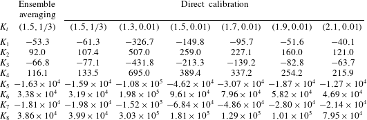
implies that the dissipation scales of salinity and temperature are comparable, and therefore such simulations could be performed using relatively modest computational grids. The results of the ensemble-averaging calibration are shown in the second column of table 1. This calculation was carried out for
 $(R_{\unicode[STIX]{x1D70C}},Pr,\unicode[STIX]{x1D70F})=(1.5,7,1/3)$
using the computational domain of
 $(L_{x},L_{z})=(300,300)$
resolved by the numerical grids of
 $(N_{x},N_{z})=(256,256)$
points. The governing equations for the basic variables
 $(\bar{T},\bar{S},\bar{\unicode[STIX]{x1D713}})$
were first integrated in time to
 $t_{00}=100$
, producing a statistically equilibrated flow field. Afterwards, the computations of basic variables were accompanied by the concurrent integrations of auxiliary functions
 $(\tilde{T}_{iT},\tilde{T}_{iS},\tilde{T}_{i\unicode[STIX]{x1D713}},\tilde{S}_{iT},\tilde{S}_{iS},\tilde{S}_{i\unicode[STIX]{x1D713}})$
. The auxiliary problems were repeatedly solved over finite intervals
 $[t_{0},t_{0}+\unicode[STIX]{x0394}T]$
, where
 $t_{0}=t_{00}+n\unicode[STIX]{x0394}T$
. The length of each integration interval was set to
 $\unicode[STIX]{x0394}T=20$
and the initial conditions
 $(\tilde{T},\tilde{S})=(0,0)$
were assumed for all auxiliary functions at the beginning of each interval. The resulting records of
 $K_{j}^{inst}(t^{\prime })$
, where
 $t^{\prime }=t-t_{0}$
, were ensemble-averaged over
 $N_{tot}=8\times 10^{5}$
realizations. The patterns of
 $K_{j}^{inst}(t^{\prime })$
exhibit the tendency to converge in time to specific equilibrium values. Their time averages over intervals
 $15<t^{\prime }<20$
were used as estimates of
 $K_{j}$
, which are listed in table 1.
Calibration of the multiscale model. The transfer coefficients
 $K_{j}~(j=1,\ldots ,8)$
are evaluated using the ensemble-averaging and the direct calibration methods for the various values (
 $\bar{\bar{R}}_{\unicode[STIX]{x1D70C}},\unicode[STIX]{x1D70F}$
) shown.

3.3 Direct calibration
While the ensemble-averaging approach is of interest in its own right, the sheer number of integrations required by this technique make its application to the oceanographically motivated case (
 $\unicode[STIX]{x1D70F}=0.01$
) unfeasible. The disparity in the dissipation scales of salinity and temperature in this regime demands a much higher resolution for
 $\unicode[STIX]{x1D70F}=0.01$
than for
 $\unicode[STIX]{x1D70F}=1/3$
, which makes ensemble-averaging prohibitively expensive even in two dimensions. To obtain the coefficients
 $K_{j}$
for such cases, we adopted the method which is referred to hereafter as direct calibration. The crux of this approach is the introduction of appropriately designed trial functions
 $T^{tr}(z)$
and
 $S^{tr}(z)$
, representing large-scale temperature and salinity fields, and the subsequent analysis of the corresponding flux-convergence patterns. For instance, in order to evaluate the coefficients
 $K_{1}$
and
 $K_{3}$
, we chose the following trial functions:
 $$\begin{eqnarray}\left.\begin{array}{@{}c@{}}T^{tr}=A((z-\frac{1}{4}L_{z})^{n}-(\frac{1}{4}L_{z})^{n})\quad \text{for }0<z<\frac{1}{2}L_{z},\\ T^{tr}=-A((z-\frac{3}{4}L_{z})^{n}-(\frac{3}{4}L_{z})^{n})\quad \text{for }\frac{1}{2}L_{z}<z<L_{z},\\ S^{tr}=0,\end{array}\right\}\end{eqnarray}$$
where
 $n=2$
. Note that the trial functions in (3.15), as well as their first derivatives, are periodic in
 $z$
and therefore compatible with the employed spectral model. The calibration was performed using high-resolution DNS, in which the
 $x$
-averaged temperature and salinity fields were reset to the trial functions (3.15) at each time step. The implementation of the resetting algorithm is particularly straightforward for our spectral model, where the
 $x$
-averages of field variables are represented by the corresponding Fourier harmonics with zero horizontal wavenumbers (
 $k_{x}=0$
). Prior to resetting the
 $T{-}S$
averages to the assumed trial functions on each step, their temporal tendencies
 $(T_{t}^{tr},S_{t}^{tr})$
are evaluated at
 $z=(1/4)L_{z}$
,
 $z=(3/4)L_{z}$
and recorded. Assuming that the temporal tendencies of the
 $x$
-averages in DNS conform to the functional form (3.12) suggested by the multiscale model, we arrive at
 $$\begin{eqnarray}\left.\begin{array}{@{}c@{}}T_{t}^{tr}|_{z=(1/4)L_{z}}=2K_{1}A,\quad T_{t}^{tr}|_{z=(3/4)L_{z}}=-2K_{1}A,\\ S_{t}^{tr}|_{z=(1/4)L_{z}}=2K_{3}A,\quad S_{t}^{tr}|_{z=(3/4)L_{z}}=-2K_{3}A.\end{array}\right\}\end{eqnarray}$$
Thus, the coefficients
 $K_{1}$
and
 $K_{3}$
can be evaluated as follows:
 $$\begin{eqnarray}K_{1}=\frac{1}{4A}[T_{t}^{tr}|_{z=(1/4)L_{z}}-T_{t}^{tr}|_{z=(3/4)L_{z}}],\quad K_{3}=\frac{1}{4A}[S_{t}^{tr}|_{z=(1/4)L_{z}}-S_{t}^{tr}|_{z=(3/4)L_{z}}],\end{eqnarray}$$
where square brackets represent averaging in time. To evaluate
 $K_{5}$
and
 $K_{7}$
, we use the trial functions (3.15) with
 $n=4$
, in which case the counterpart of (3.17) becomes
 $$\begin{eqnarray}K_{5}=\frac{1}{48A}[T_{t}^{tr}|_{z=(1/4)L_{z}}-T_{t}^{tr}|_{z=(3/4)L_{z}}],\quad K_{7}=\frac{1}{48A}[S_{t}^{tr}|_{z=(1/4)L_{z}}-S_{t}^{tr}|_{z=(3/4)L_{z}}].\end{eqnarray}$$
The coefficients
 $(K_{2},K_{4},K_{6},K_{8})$
were similarly calibrated by assuming the trial functions which represent variation in the salinity stratification:
 $$\begin{eqnarray}\left.\begin{array}{@{}c@{}}S^{tr}=A((z-\frac{1}{4}L_{z})^{n}-(\frac{1}{4}L_{z})^{n})\quad \text{for }0<z<\frac{1}{2}L_{z},\\ S^{tr}=-A((z-\frac{3}{4}L_{z})^{n}-(\frac{3}{4}L_{z})^{n})\quad \text{for }\frac{1}{2}L_{z}<z<L_{z},\\ T^{tr}=0,\end{array}\right\}\end{eqnarray}$$
where
 $n=2$
was used to evaluate
 $K_{2}$
and
 $K_{4}$
, while
 $n=4$
led to the estimate of
 $K_{6}$
and
 $K_{8}$
.
The coefficients
 $K_{j}$
evaluated using direct calibration are listed in table 1 for a series of simulations performed for various values of
 $(R_{\unicode[STIX]{x1D70C}},\unicode[STIX]{x1D70F})$
. Each calculation was extended in time long enough to obtain reliable statistically steady temporal averages of
 $(T_{t}^{tr},S_{t}^{tr})$
. The computational domain chosen for those simulations was rather large, particularly in terms of its vertical extent:
 $(L_{x},L_{z})=(200,400)$
. This choice ensured that the obtained values of
 $K_{j}$
are consistent with the multiscale model, which assumes clear scale separation between microstructure and slowly evolving large-scale modes of interest.
The direct calibration procedure has been validated by comparing its predictions with the corresponding estimates based on the ensemble-averaging method (§ 3.2). For this, the direct calibration technique was first applied to the computationally convenient case of
 $\unicode[STIX]{x1D70F}=1/3$
. The resulting values of
 $K_{j}$
obtained using ensemble-averaging and direct calibration are listed in columns two and three of table 1, respectively. The results are mutually consistent, which instils confidence in the adequate performance of both models. However, due to computational constraints, no ensemble-averaging results are available for the oceanographically relevant case of
 $\unicode[STIX]{x1D70F}=0.01$
, which is the primary focus of our investigation. Therefore, all subsequent developments are based exclusively on the direct calibration method. The calculations of
 $K_{j}$
in this regime were performed using the numerical mesh with
 $(N_{x},N_{z})=(1536,3072)$
grid points, which made it possible to resolve the dissipation scale of salinity.
4 Large-scale solutions
The objective of this section is the analysis of large-scale solutions of the parametric system (3.12) and comparison of the results with corresponding estimates based on the more conventional flux-gradient laws (e.g. Stern et al. Reference Stern, Radko and Simeonov2001; Radko Reference Radko2003; Traxler et al. Reference Traxler, Stellmach, Garaud, Radko and Brummel2011). The flux-gradient model, written in our non-dimensional units (e.g. Radko Reference Radko2014), takes the form
 $$\begin{eqnarray}\left.\begin{array}{@{}c@{}}\displaystyle \frac{\unicode[STIX]{x2202}T_{0}}{\unicode[STIX]{x2202}t}=\frac{\unicode[STIX]{x2202}}{\unicode[STIX]{x2202}z}\left(Nu\left(1+\frac{\unicode[STIX]{x2202}T_{0}}{\unicode[STIX]{x2202}z}\right)\right),\\ \displaystyle \frac{\unicode[STIX]{x2202}S_{0}}{\unicode[STIX]{x2202}t}=\frac{\unicode[STIX]{x2202}}{\unicode[STIX]{x2202}z}\left(\frac{Nu}{\unicode[STIX]{x1D6FE}}\left(1+\frac{\unicode[STIX]{x2202}T_{0}}{\unicode[STIX]{x2202}z}\right)\right),\end{array}\right\}\end{eqnarray}$$
where
 $Nu$
is the Nusselt number and
 $\unicode[STIX]{x1D6FE}$
is the flux ratio. Both
 $Nu$
and
 $\unicode[STIX]{x1D6FE}$
are assumed to be controlled by the local large-scale density ratio, which in non-dimensional units reduces to
 $$\begin{eqnarray}R_{\unicode[STIX]{x1D70C}}=\left.\left(1+\frac{\unicode[STIX]{x2202}T_{0}}{\unicode[STIX]{x2202}z}\right)\right/\left(\frac{1}{\bar{\bar{R}}_{\unicode[STIX]{x1D70C}}}+\frac{\unicode[STIX]{x2202}S_{0}}{\unicode[STIX]{x2202}z}\right).\end{eqnarray}$$
Based on a suite of high-resolution two-dimensional DNS and theoretical arguments, Radko (Reference Radko2014) suggested the following specific parametrizations for
 $Nu$
and
 $\unicode[STIX]{x1D6FE}$
:
 $$\begin{eqnarray}\left.\begin{array}{@{}c@{}}\displaystyle \unicode[STIX]{x1D6FE}\approx a_{\unicode[STIX]{x1D6FE}}\exp (b_{\unicode[STIX]{x1D6FE}}R_{\unicode[STIX]{x1D70C}})+c_{\unicode[STIX]{x1D6FE}},\quad (a_{\unicode[STIX]{x1D6FE}},b_{\unicode[STIX]{x1D6FE}},c_{\unicode[STIX]{x1D6FE}})=(4.752,-3.318,0.59),\\ \displaystyle Nu=\unicode[STIX]{x1D6FE}\left(\frac{a_{S}}{\sqrt{R_{\unicode[STIX]{x1D70C}}-1}}+b_{S}\right),\quad (a_{S},b_{S})=(136.9,-105.13).\end{array}\right\}\end{eqnarray}$$
In order to facilitate the direct comparison of the growth rates realized in the flux-gradient formulation and in the foregoing multiscale model, the formulation (4.1) was linearized with respect to the uniform background
 $T{-}S$
gradient by assuming that the large-scale perturbations are weak:
 $(\unicode[STIX]{x2202}T_{0}/\unicode[STIX]{x2202}z),(\unicode[STIX]{x2202}S_{0}/\unicode[STIX]{x2202}z)\ll 1$
. The linearization reduces (4.1) to
 $$\begin{eqnarray}\left.\begin{array}{@{}c@{}}\displaystyle \frac{\unicode[STIX]{x2202}T_{0}}{\unicode[STIX]{x2202}t}=K_{1fg}\frac{\unicode[STIX]{x2202}^{2}T_{0}}{\unicode[STIX]{x2202}z^{2}}+K_{2fg}\frac{\unicode[STIX]{x2202}^{2}S_{0}}{\unicode[STIX]{x2202}z^{2}},\\ \displaystyle \frac{\unicode[STIX]{x2202}S_{0}}{\unicode[STIX]{x2202}t}=K_{3fg}\frac{\unicode[STIX]{x2202}^{2}T_{0}}{\unicode[STIX]{x2202}z^{2}}+K_{4fg}\frac{\unicode[STIX]{x2202}^{2}S_{0}}{\unicode[STIX]{x2202}z^{2}},\end{array}\right\}\end{eqnarray}$$
where
 $$\begin{eqnarray}\left.\begin{array}{@{}c@{}}\displaystyle K_{1fg}=\left.\left(R_{\unicode[STIX]{x1D70C}}\frac{\unicode[STIX]{x2202}Nu}{\unicode[STIX]{x2202}R_{\unicode[STIX]{x1D70C}}}+Nu\right)\right|_{R_{\unicode[STIX]{x1D70C}}=\bar{\bar{R}}_{\unicode[STIX]{x1D70C}}},\quad K_{2fg}=\left.\left(-R_{\unicode[STIX]{x1D70C}}^{2}\frac{\unicode[STIX]{x2202}Nu}{\unicode[STIX]{x2202}R_{\unicode[STIX]{x1D70C}}}\right)\right|_{R_{\unicode[STIX]{x1D70C}}=\bar{\bar{R}}_{\unicode[STIX]{x1D70C}}},\\ \displaystyle K_{3fg}=\left.\left(R_{\unicode[STIX]{x1D70C}}\frac{\unicode[STIX]{x2202}(\unicode[STIX]{x1D6FE}^{-1})}{\unicode[STIX]{x2202}R_{\unicode[STIX]{x1D70C}}}Nu+\frac{R_{\unicode[STIX]{x1D70C}}}{\unicode[STIX]{x1D6FE}}\frac{\unicode[STIX]{x2202}Nu}{\unicode[STIX]{x2202}R_{\unicode[STIX]{x1D70C}}}+\frac{Nu}{\unicode[STIX]{x1D6FE}}\right)\right|_{R_{\unicode[STIX]{x1D70C}}=\bar{\bar{R}}_{\unicode[STIX]{x1D70C}}},\\ \displaystyle K_{4fg}=\left.\left(-R_{\unicode[STIX]{x1D70C}}^{2}\frac{\unicode[STIX]{x2202}(\unicode[STIX]{x1D6FE}^{-1})}{\unicode[STIX]{x2202}R_{\unicode[STIX]{x1D70C}}}Nu-\frac{R_{\unicode[STIX]{x1D70C}}^{2}}{\unicode[STIX]{x1D6FE}}\frac{\unicode[STIX]{x2202}Nu}{\unicode[STIX]{x2202}R_{\unicode[STIX]{x1D70C}}}\right)\right|_{R_{\unicode[STIX]{x1D70C}}=\bar{\bar{R}}_{\unicode[STIX]{x1D70C}}}.\end{array}\right\}\end{eqnarray}$$
Even a casual inspection of (4.4) and (3.12) indicates that the two formulations are structurally similar. The fundamental difference between them is the notable absence of the fourth-order derivatives in the flux-gradient model – components reflecting the influence of non-uniformities of large-scale
 $T{-}S$
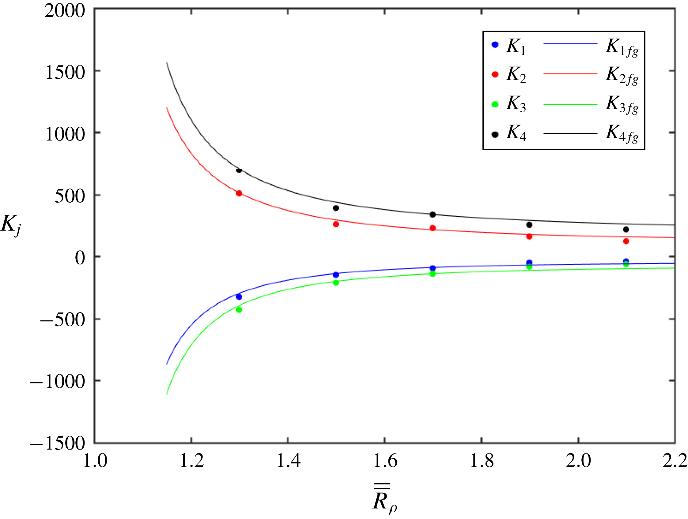
gradients on vertical fluxes. To make this comparison more quantitative, in figure 2 we plot the flux-gradient coefficients
 $K_{jfg},~j=1,\ldots ,4$
, evaluated using (4.3) and (4.5) as a function of the density ratio (
 $\bar{\bar{R}}_{\unicode[STIX]{x1D70C}}$
). Superimposed on the flux-gradient coefficients are the corresponding values of
 $K_{j}$
obtained from the calibration of the multiscale model (table 1). The general agreement between the two estimates indicates that the flux-gradient and multiscale models are mutually consistent in terms of representing the effects of large-scale property gradients. The multiscale model, however, presents a unique opportunity to move beyond the flux-gradient formulation and adjust the flux laws by including a correction associated with non-uniformities of property gradients. Since the coefficients
 $K_{j},~j=5,\ldots ,8$
, representing such non-uniformities have been evaluated for a discrete set of density ratios (table 1), it also becomes desirable to formulate a consistent model of
 $K_{j}(\bar{\bar{R}}_{\unicode[STIX]{x1D70C}})$
for a continuous range of
 $\bar{\bar{R}}_{\unicode[STIX]{x1D70C}}$
. This was accomplished by assuming the following closure form, motivated by theoretical arguments in Radko (Reference Radko2008):
 $$\begin{eqnarray}K_{j}(\bar{\bar{R}}_{\unicode[STIX]{x1D70C}})=\frac{a_{j}}{\sqrt{\bar{\bar{R}}_{\unicode[STIX]{x1D70C}}-1}}+b_{j},\quad j=5,\ldots ,8.\end{eqnarray}$$
The transfer coefficients
 $K_{j\,fg},~j=1,\ldots ,4$
, obtained using the parametric flux-gradient model (solid curves) are plotted as a function of the background density ratio
 $\bar{\bar{R}}_{\unicode[STIX]{x1D70C}}$
along with the corresponding estimates obtained using the multiscale model (
 $K_{j}$
) which are indicated by dots.

The coefficients
 $(a_{j},b_{j})$
were evaluated from the best fit of (4.6) to the values of
 $K_{j},~j=5,\ldots ,8$
, listed in table 1:
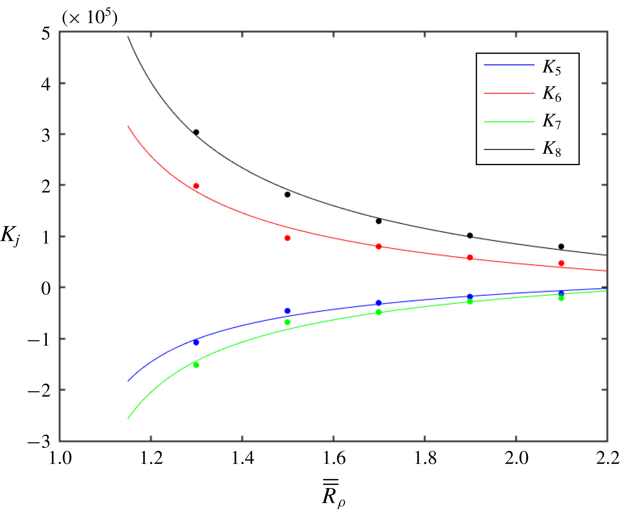
 $$\begin{eqnarray}\left.\begin{array}{@{}c@{}}a_{5}=-1.09\times 10^{5},\quad a_{6}=1.70\times 10^{5},\quad a_{7}=-1.49\times 10^{5},\quad a_{8}=-2.56\times 10^{5},\\ b_{5}=9.71\times 10^{4},\quad b_{6}=-1.23\times 10^{5},\quad b_{7}=1.29\times 10^{5},\quad b_{8}=-1.72\times 10^{5}.\\ \end{array}\right\}\end{eqnarray}$$
The resulting patterns of
 $K_{j}(\bar{\bar{R}}_{\unicode[STIX]{x1D70C}})$
are shown in figure 3, along with the corresponding discrete estimates derived from the multiscale model.
The biharmonic transfer coefficients
 $K_{j},~j=5,\ldots ,8$
, obtained using the multiscale model (dots) are plotted as a function of the background density ratio
 $\bar{\bar{R}}_{\unicode[STIX]{x1D70C}}$
along with the corresponding empirical parametrization (4.6).

Having formulated the generalized flux laws, we now proceed to explore the corresponding large-scale solutions. Of particular interest are the growth rates of long-wavelength perturbations (
 $\unicode[STIX]{x1D706}$
) and their dependence on wavenumbers (
 $m$
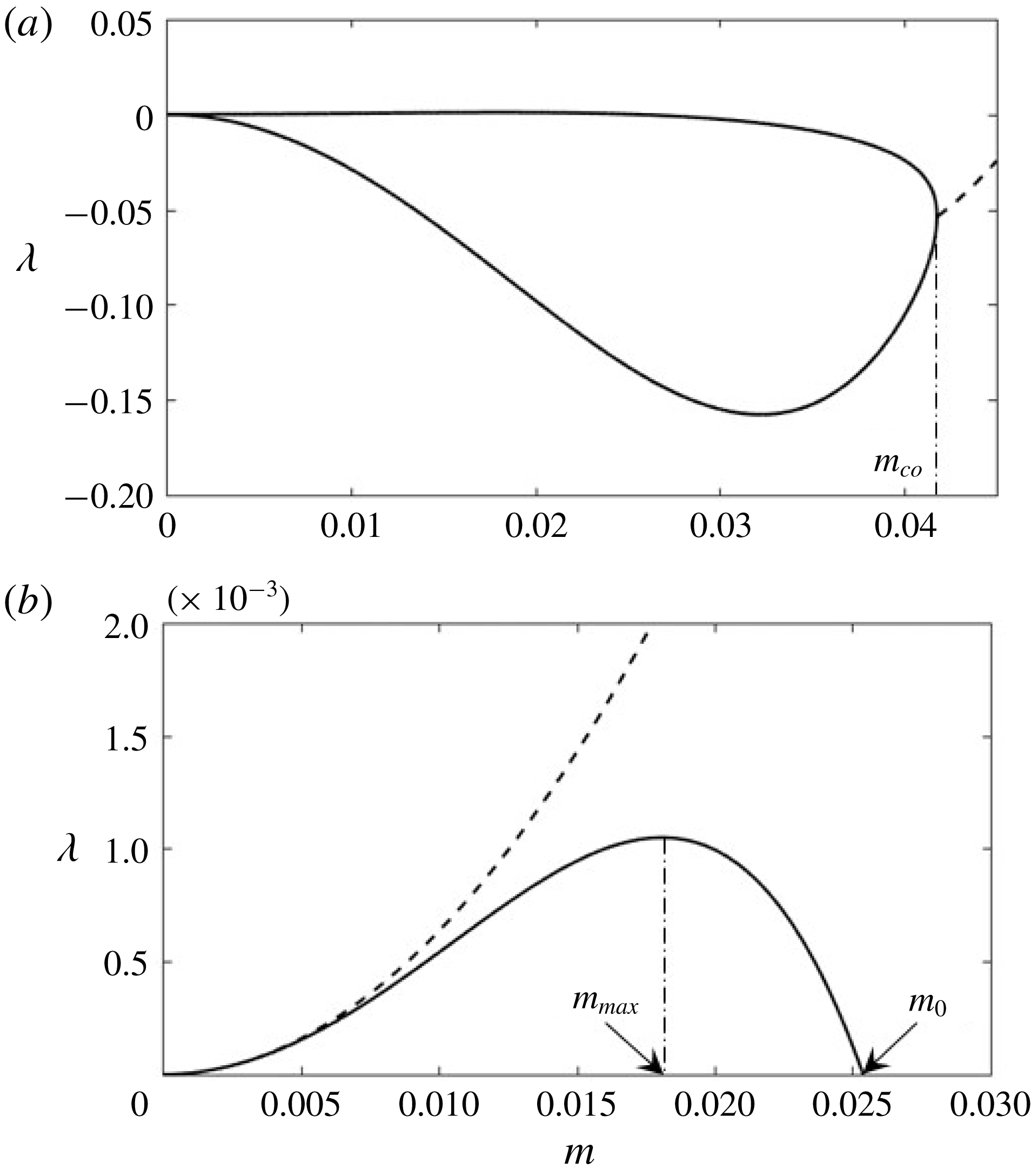
). A typical growth rate pattern
 $\unicode[STIX]{x1D706}(m)$
is shown in figure 4(a), where
 $\unicode[STIX]{x1D706}$
was computed using (3.14) for
 $\bar{\bar{R}}_{\unicode[STIX]{x1D70C}}=1.5$
. For small
 $m$
, the growth rates are characterized by two real solutions. These branches coalesce at the bifurcation point
 $m_{co}$
, and for
 $m>m_{co}$
, the growth rate attains a substantial imaginary component. Recalling that (i) the multiscale theory leading to (3.12) has been developed within the context of long-wave approximation (
 $m\ll 1$
) and (ii) the microstructure-resolving DNS exhibit no evidence of oscillatory variation of large-scale components, we assume that the obtained flux laws become inapplicable for
 $m>m_{co}$
. Thus, the bifurcation point
 $m_{co}$
is interpreted as a natural cutoff scale for the validity of the proposed model.
(a) The stability diagram for the basic state with
 $(\bar{\bar{R}}_{\unicode[STIX]{x1D70C}},Pr,\unicode[STIX]{x1D70F})=(1.5,7,0.01)$
. The solid curves represent solutions of (3.14) with real growth rates (
 $\unicode[STIX]{x1D706}$
), which are realized for small wavenumbers (
 $m<m_{co}$
). For large wavenumbers (
 $m>m_{co}$
) the growth rates attain imaginary components and their real part is indicated by the dashed curve. (b) The enlarged view of the stability diagram in (a), which is focused on the region with positive growth rates. The wavenumber corresponding to the maximal growth rate is denoted by
 $m_{max}$
, whereas
 $m_{0}$
represents the wavenumber of the mode with zero growth rate.

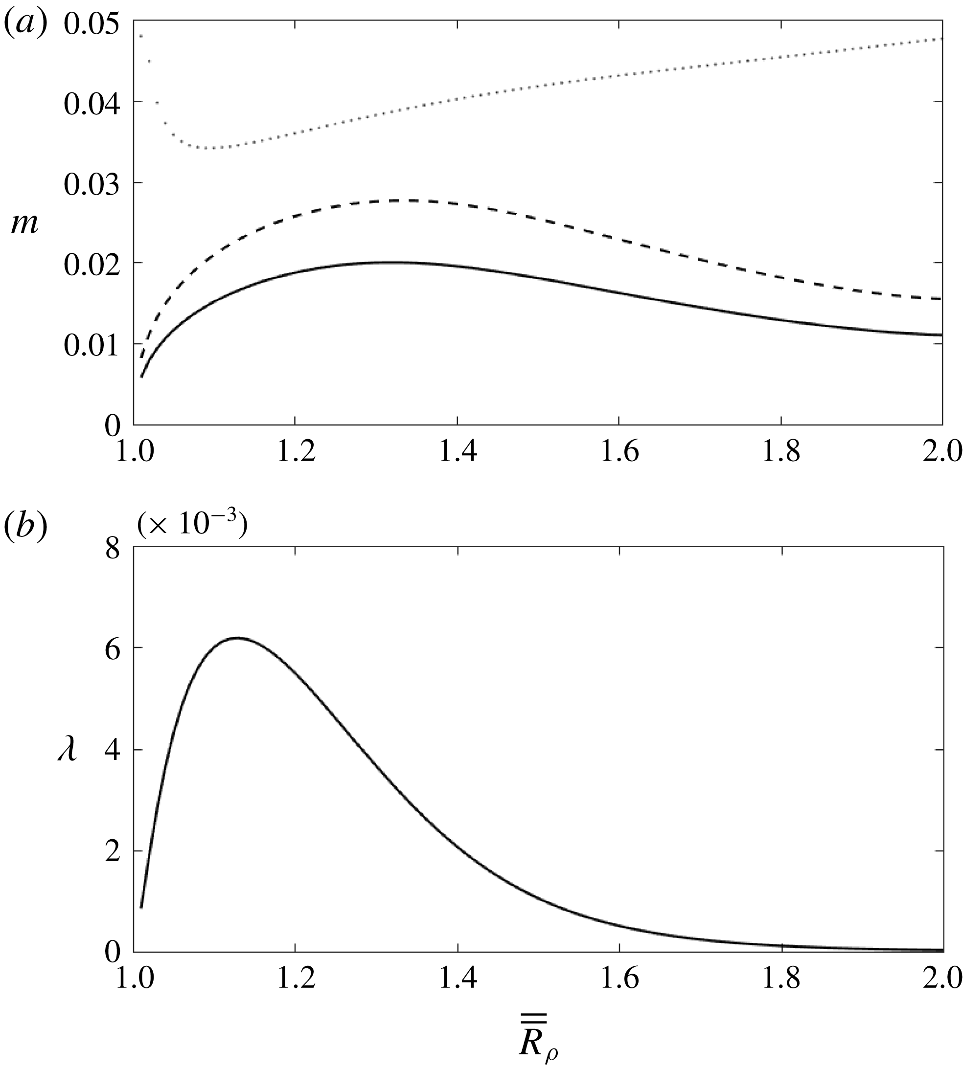
(a) The wavenumbers of the most rapidly amplifying mode (
 $m_{max}$
) and the mode of zero growth rate (
 $m_{0}$
), as well as the cutoff wavenumber (
 $m_{co}$
), are plotted as a function of the background density ratio
 $\bar{\bar{R}}_{\unicode[STIX]{x1D70C}}$
using solid, dashed and dotted curves, respectively. (b) The maximal growth rate of layering modes as a function of the density ratio.

One of the key questions our study attempts to address is the selection of the preferred wavelength of layering modes. Therefore, in figure 4(b) we present an enlarged view of the growth rate pattern (figure 4
a) which is focused on the region with positive values of
 $\unicode[STIX]{x1D706}$
. For our investigation, the most significant feature of the relation in figure 4(b) is the presence of the maximum in the growth rate at
 $m=m_{max}$
, representing the most rapidly amplifying large-scale mode. Figure 4(b) also presents (dashed curve) the corresponding prediction based on the flux-gradient model (e.g. Radko Reference Radko2003). While the flux-gradient and multiscale models are mutually consistent for very small wavenumbers (
 $m<0.01$
), their agreement rapidly deteriorates for larger values of
 $m$
. Unlike the generalized model, the flux-gradient theory predicts the growth rate
 $\unicode[STIX]{x1D706}(m)$
which monotonically increases with wavenumber, making it impossible to evaluate the spatial and temporal scales of dominant layering modes. The generalized model (3.12), on the other hand, offers a reasonable estimate of relevant scales of layering instability. For instance, the fastest-growing mode realized in the foregoing DNS (figure 1) is characterized by the wavenumber of
 $m_{max}=3.14\times 10^{-2}$
and the corresponding growth rate of
 $\unicode[STIX]{x1D706}_{max}=1.56\times 10^{-3}$
. These values are broadly consistent – within a factor of two – with the estimate based on the multiscale model (figure 4
b):
 $m_{max}=1.81\times 10^{-2}$
and
 $\unicode[STIX]{x1D706}_{max}=1.05\times 10^{-3}$
.
To explore the variation in the stability characteristics of layering modes with the background density ratio, in figure 5(a) we present the
 $m_{max}(\bar{\bar{R}}_{\unicode[STIX]{x1D70C}})$
relation, as well as the corresponding patterns of the zero-growth-rate wavenumber
 $(m_{0})$
and the cutoff wavenumber
 $(m_{co})$
. Figure 5(a) indicates that the wavenumber of the most rapidly amplifying mode
 $(m_{max})$
exhibits a rather modest sensitivity to
 $\bar{\bar{R}}_{\unicode[STIX]{x1D70C}}$
, varying at most by a factor of two in the range of
 $1<\bar{\bar{R}}_{\unicode[STIX]{x1D70C}}<2$
. The variation in the maximal growth rate (figure 5
b) is much stronger. The growth rates can be as high as
 $\unicode[STIX]{x1D706}\sim 6\times 10^{-3}$
for
 $\bar{\bar{R}}_{\unicode[STIX]{x1D70C}}=1.2$
, which corresponds to the dimensional amplification time scale of a day, and as low as
 $\unicode[STIX]{x1D706}\sim 2.5\times 10^{-5}$
for
 $\bar{\bar{R}}_{\unicode[STIX]{x1D70C}}=2$
, dimensionally equivalent to the time scale of a year. It should be mentioned at this point that the majority of fingering staircases observed in the ocean are characterized by relatively low density ratios
 $1.1<\bar{\bar{R}}_{\unicode[STIX]{x1D70C}}<1.7$
, as summarized, for example, by Radko (Reference Radko2013). This property could be a consequence of the dramatic reduction in the growth rates of layering modes for large
 $\bar{\bar{R}}_{\unicode[STIX]{x1D70C}}$
in figure 5(b).
5 The parametric model of thermohaline staircases
While the previous section addressed the linear stability of layering modes, a question arises whether the proposed model can adequately represent the transition of weakly perturbed large-scale gradients to fully developed staircases (e.g. figure 1). Since the following discussion is exclusively focused on the dynamics of large-scale stratification, we shall abandon the rather cumbersome double-bar notation, as well as subscripts ‘0’, representing the leading-order terms in asymptotic expansion. To place our results in the context of oceanic observations, the following results will be expressed exclusively in dimensional units and the asterisks, previously denoting dimensional variables, will be omitted. The conversion between dimensional and non-dimensional units (§ 2) assumes the following parameters:
 $$\begin{eqnarray}k_{T}=1.4\times 10^{-7}~\text{m}^{2}~\text{s}^{-1},\quad \unicode[STIX]{x1D708}=10^{-6}~\text{m}^{2}~\text{s}^{-1},\quad g=9.8~\text{m}~\text{s}^{-2},\quad \unicode[STIX]{x1D6FC}=2\times 10^{-4}~\text{K}^{-1},\end{eqnarray}$$
which are representative of typical oceanic conditions.
The proposed parametric model integrates the one-dimensional evolutionary equations based on the generalized flux laws introduced in §§ 3 and 4:
 $$\begin{eqnarray}\left.\begin{array}{@{}c@{}}\displaystyle \frac{\unicode[STIX]{x2202}T}{\unicode[STIX]{x2202}t}=k_{T}\frac{\unicode[STIX]{x2202}}{\unicode[STIX]{x2202}z}\left(Nu(R_{\unicode[STIX]{x1D70C}})\frac{\unicode[STIX]{x2202}(T_{bg}+T)}{\unicode[STIX]{x2202}z}\right)+k_{T}d^{2}K_{5}(R_{\unicode[STIX]{x1D70C}})\frac{\unicode[STIX]{x2202}^{4}T}{\unicode[STIX]{x2202}z^{4}}+k_{T}d^{2}\frac{\unicode[STIX]{x1D6FD}}{\unicode[STIX]{x1D6FC}}K_{6}(R_{\unicode[STIX]{x1D70C}})\frac{\unicode[STIX]{x2202}^{4}S}{\unicode[STIX]{x2202}z^{4}},\\ \displaystyle \frac{\unicode[STIX]{x2202}S}{\unicode[STIX]{x2202}t}=k_{T}\frac{\unicode[STIX]{x1D6FC}}{\unicode[STIX]{x1D6FD}}\frac{\unicode[STIX]{x2202}}{\unicode[STIX]{x2202}z}\left(\frac{Nu(R_{\unicode[STIX]{x1D70C}})}{\unicode[STIX]{x1D6FE}(R_{\unicode[STIX]{x1D70C}})}\frac{\unicode[STIX]{x2202}(T_{bg}+T)}{\unicode[STIX]{x2202}z}\right)+k_{T}d^{2}\frac{\unicode[STIX]{x1D6FC}}{\unicode[STIX]{x1D6FD}}K_{7}(R_{\unicode[STIX]{x1D70C}})\frac{\unicode[STIX]{x2202}^{4}T}{\unicode[STIX]{x2202}z^{4}}+k_{T}d^{2}K_{8}(R_{\unicode[STIX]{x1D70C}})\frac{\unicode[STIX]{x2202}^{4}S}{\unicode[STIX]{x2202}z^{4}},\\ \displaystyle R_{\unicode[STIX]{x1D70C}}=\left.\left(\unicode[STIX]{x1D6FC}\frac{\unicode[STIX]{x2202}(T_{bg}+T)}{\unicode[STIX]{x2202}z}\right)\right/\left(\unicode[STIX]{x1D6FD}\frac{\unicode[STIX]{x2202}(S_{bg}+S)}{\unicode[STIX]{x2202}z}\right),\quad d=\left(k_{T}\unicode[STIX]{x1D708}\left/\left(g\unicode[STIX]{x1D6FC}\frac{\unicode[STIX]{x2202}(T_{bg}+T)}{\unicode[STIX]{x2202}z}\right)\right.\right)^{1/4}.\end{array}\right\}\end{eqnarray}$$
The flux-gradient components of evolutionary equations (5.2) are identical to those used in our previous investigations (Radko Reference Radko2005, Reference Radko2014). These terms are fully consistent with the estimates based on the multiscale model (e.g. figure 2) and therefore no adjustment of the flux-gradient module is necessary. The biharmonic components in (5.2) are introduced using the multiscale-derived formulation (4.6) in an attempt to correct unphysical features of the flux-gradient model. The governing equations were integrated in time using a spectral model analogous to that employed in Radko (Reference Radko2005, Reference Radko2007). At each time step, the Fourier harmonics with wavenumbers exceeding the cutoff scale for the validity of the multiscale model (
 $m_{co}$
) were set to zero. The evolving temperature and salinity fields eventually produce convective top-heavy regions
 $(\unicode[STIX]{x2202}\unicode[STIX]{x1D70C}_{tot}/\unicode[STIX]{x2202}z>0)$
, which is a generic and well-documented property of fully developed thermohaline staircases (e.g. Krishnamurti Reference Krishnamurti2009 and Stellmach et al.
Reference Stellmach, Traxler, Garaud, Brummell and Radko2011). To represent dynamics of these regions, we implemented a simple iterative procedure, which replaces the
 $T{-}S$
profiles in convectively unstable intervals by the uniform values of temperature and salinity corresponding to their spatial averages over the extent of each convecting zone.
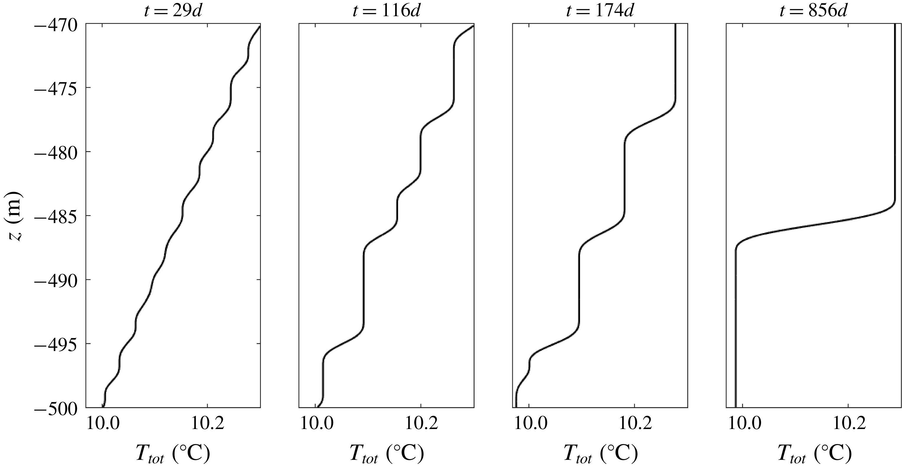
The evolution of the vertical temperature profile in the one-dimensional parametric model. Note the spontaneous appearance of well-defined layers and their subsequent mergers. For ease of comparison with oceanographic measurements, the total temperature and depth are referenced to
 $T_{tot}\sim 10\,^{\circ }\text{C}$
and
 $z\sim -500$
m – values representative of staircases in the main thermocline.

Figure 6 presents a typical solution of the proposed model. This simulation was performed using the uniform background gradient with
 $$\begin{eqnarray}\frac{\unicode[STIX]{x2202}T_{bg}}{\unicode[STIX]{x2202}z}=0.01\,^{\circ }\text{C}~\text{m}^{-1},\quad R_{\unicode[STIX]{x1D70C}\,bg}\equiv \left.\left(\unicode[STIX]{x1D6FC}\frac{\unicode[STIX]{x2202}T_{bg}}{\unicode[STIX]{x2202}z}\right)\right/\left(\unicode[STIX]{x1D6FD}\frac{\unicode[STIX]{x2202}S_{bg}}{\unicode[STIX]{x2202}z}\right)=1.5.\end{eqnarray}$$
The computational domain of
 $L_{z}=30$
m was resolved by
 $N_{z}=1024$
grid points and a small-amplitude random perturbation was used as the initial condition for
 $T$
and
 $S$
. The integration of the governing equations in time reveals three distinct evolutionary stages. The first stage (
 $t<10~\text{days}$
) represents the linear growth of unstable modes, in which the perturbation becomes dominated by the most rapidly amplifying mode with the wavelength of 3 m. During the layering phase (
 $10~\text{days}<t<25~\text{days}$
), this mode transforms into a well-defined staircase, consisting of 10 convecting layers, separated by high-gradient double-diffusive interfaces. The subsequent evolution of the staircase (
 $t>25~\text{days}$
) is characterized by the sequential mergers of layers, which systematically decrease the number of layers and increase their average height. After two years, the system evolves to the stable configuration with only one layer within the limits of our computational domain.
The merging dynamics revealed by figure 6 appears to be a rather common evolutionary feature of thermohaline staircases (e.g. Zodiatis & Gasparini Reference Zodiatis and Gasparini1996; Radko Reference Radko2005; Radko et al.
Reference Radko, Flanagan, Stellmach and Timmermans2014). In particular, Radko (Reference Radko2007) proposed to classify all layer-merging events into two categories: (i)
 $B$
-mergers, characterized by strengthening of stronger interfaces at the expense of weaker ones, which gradually erode and eventually disappear; and (ii)
 $H$
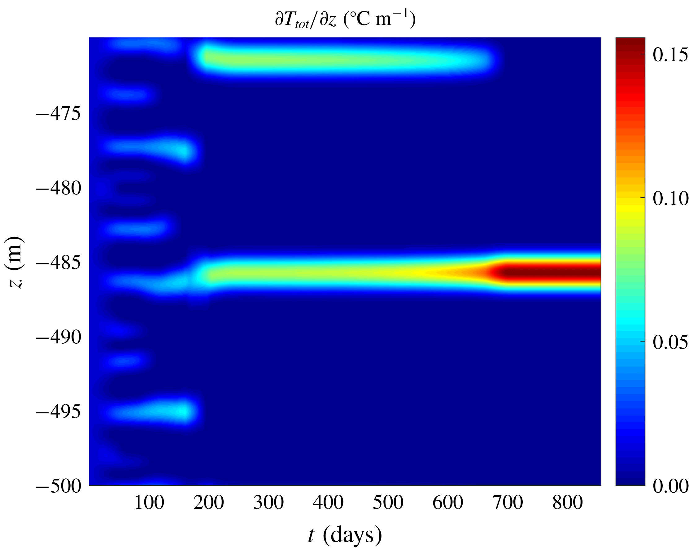
-mergers, associated with the vertical drift and coalescence of high-gradient interfaces. In order to determine the prevailing merging mechanism in our one-dimensional parametric model, in figure 7 we present the Hovmöller (space–time) diagram of the vertical temperature gradient
 $(\unicode[STIX]{x2202}T_{tot}/\unicode[STIX]{x2202}z)$
. Figure 7 clearly reveals that the modelled staircase evolves through a series of
 $B$
-mergers. While the interfaces tend to maintain their position, the
 $T{-}S$
variations across interfaces change significantly in time. As a result, the relatively weak interfaces successively vanish. While
 $B$
-mergers are perhaps more widespread (e.g. Radko et al.
Reference Radko, Flanagan, Stellmach and Timmermans2014), there are known examples of
 $H$
-merger-dominated evolution, such as the coarsening of diffusive staircases in the presence of large-scale external shear (Radko Reference Radko2016b
). An interesting and largely unresolved question concerns the processes that ultimately arrest the mergers of layers and lead to the formation of stable quasi-steady staircases. Radko (Reference Radko2005) suggested that the critical height of layers beyond which mergers cease – and even the very existence of such equilibrium height – is highly sensitive to the chosen parametrization of convection in well-mixed layers. Therefore, our ability to formulate a reliable predictive theory for the equilibrium height of layers is contingent on the availability of accurate convective laws, the development of which is in itself a broad and active area of research (e.g. Grossmann & Lohse Reference Grossmann and Lohse2000; Ahlers, Grossmann & Lohse Reference Ahlers, Grossmann and Lohse2009).
The Hovmöller (space–time) diagram of the temperature gradient for the experiment in figure 6. Note the sequential mergers of layers associated with the growth of relatively strong interfaces at the expense of weaker interfaces which gradually decay and eventually disappear (the
 $B$
-merger mechanism).

6 Discussion
A fundamental problem in double-diffusive convection theory concerns the development of flux laws, representing the influence of primary double-diffusive instabilities on larger scales of motion. So far, this research area was dominated by the analysis and application of flux-gradient laws, which assume a unique relation between the finger-driven
 $T{-}S$
transport and vertical property gradients. The models based on flux-gradient laws are commonly used to explain the dynamics of secondary double-diffusive structures, including staircases, thermohaline intrusions and collective instability waves. While such models perform adequately in systems characterized by clear scale separation between double-diffusive microstructure and phenomena of interest, they become increasingly unreliable when the scale separation is limited.
The case in point is the theory of thermohaline staircases. The previous attempts to conceptualize thermohaline layering on the basis of flux-gradient laws have yielded promising but incomplete results. The flux-gradient model (Radko Reference Radko2003; Stellmach et al. Reference Stellmach, Traxler, Garaud, Brummell and Radko2011) revealed that smoothly stratified temperature and salinity fields are susceptible to the so-called gamma-instability. It was shown that amplifying gamma-instability modes eventually transform the background stratification into a series of homogeneous convecting layers separated by thin high-gradient interfaces – structures that are reminiscent of the observed thermohaline staircases. Unfortunately, the success of the flux-gradient model in explaining the general origin of staircases is substantially hindered by its inability to represent some of the most basic properties of layering. For instance, the flux-gradient laws lead to the erroneous conclusion that the growth rate of layering modes monotonically increases with increasing wavenumber. This unphysical feature makes the flux-gradient model fundamentally unsuitable for predicting the wavelengths of dominant layering modes and their growth rates.
The present investigation attempts to correct the apparent limitations of the flux-gradient model. We explore the possibility that the vertical eddy fluxes of heat and salt are not uniquely determined by local large-scale gradients but are also affected by the non-uniformities of
 $T{-}S$
stratification. To take these effects into account, we employed the method of multiscale analysis, which involves rewriting the governing equations using two sets of spatial and temporal variables. In our case, the first set of variables represents microscale variability driven by primary double-diffusive instability and the second set describes much larger layering modes. The key step in the development of multiscale theory is the derivation of solvability conditions which describe the evolution of the system entirely on large scales. The application of the multiscale method to the problem of thermohaline layering made it possible to formulate the generalized flux laws, which take into account the effects of the non-uniformity of large-scale stratification. Stability analysis of the doubly stratified basic state using the generalized flux model confirmed its superiority to the flux-gradient parametrization. The proposed model alleviated the complications associated with the ultraviolet catastrophe of flux-gradient laws, making it possible to predict the wavelength and time scale of dominant layering modes. These predictions are consistent with – and can be used to rationalize – the layering dynamics revealed by microstructure-resolving DNS. With regard to the analysis of the wavelength of dominant layering modes, it should be noted that the results obtained do not resolve completely the question of step-size selection in fully equilibrated staircases. The staircase dynamics is confounded by layer-merging events, which commonly occur in young evolving staircases and which systematically increase the average layer height. Nevertheless, the determination of the initial step heights offers a starting point for the analysis and places a lower bound on this elusive characteristic.
Finally, it should be emphasized that, while the specific questions addressed here are narrowly focused on the problem of thermohaline layering, the broader implications of our study could be more fundamental and far-reaching. The problems involving the interaction between phenomena operating on dissimilar spatial and temporal scales are most common in fluid mechanics – see, for example, the discussion in Mei & Vernescu (Reference Mei and Vernescu2010). Numerous examples include the propagation of sound waves through inhomogeneous fluids, the interaction of planetary-scale circulations in the oceans and atmospheres with geostrophic turbulence, and the dynamics of porous media. In each application, the principal theoretical challenge is the development of physically consistent representations of small-scale effects on larger scales of motion. Such problems are usually solved on a case-by-case basis. However, it is our belief that the success of a fairly generic multiscale approach adopted in the present study could further stimulate the development of analogous models in other fluid dynamical applications.
Acknowledgements
The author thanks N. Balmforth, J. Brown and the reviewers for helpful comments. Support of the National Science Foundation (grants OCE 1334914 and OCE 1756491) is gratefully acknowledged. The computing resources were supplied by the Extreme Science and Engineering Discovery Environment (XSEDE) programme through allocation TG-OCE110011.