1 Introduction
The Rayleigh–Taylor instability (Rayleigh Reference Rayleigh1883; Taylor Reference Taylor1950) occurs across density interfaces in fluids when an acceleration is applied such that the resulting pressure gradient opposes the density gradient. For unstable configurations, even infinitesimally small perturbations on the interface will grow with time due to the deposition of baroclinic vorticity. This continuous generation of vorticity leads to a pattern of bubbles of light fluid penetrating the heavy fluid, and spikes of heavy fluid penetrating the light fluid. These bubbles and spikes may eventually develop into a turbulent mixing layer. This Rayleigh–Taylor instability (RTI) is of great fundamental interest in fluid mechanics and physics. It has been attributed to a wide range of phenomena, from the dynamics of solidifying magma (Michioka & Sumita Reference Michioka and Sumita2005), to the filaments of the Crab nebula (Hester et al. Reference Hester, Stone, Scowen, Jun, Gallagher, Norman, Ballester, Burrows, Casertano and Clarke1996). RTI is one of the major obstacles in attaining positive net-yield inertial confinement fusion (ICF), occurring twice during the implosion process: at the outer surface when the shell is accelerated inwards, and at the hotspot–fuel interface during deceleration at the end of the implosion (Town et al. Reference Town, Delettrez, Epstein, Goncharov, McCrory, McKenty, Short and Skupsky1999). The performance of ICF is degraded by RTI mixing, which cools the central hotspot (Edwards et al. Reference Edwards, Lindl, Spears, Weber, Atherton, Bleuel, Bradley, Callahan, Cerjan and Clark2011).
Rayleigh (Reference Rayleigh1883) first examined the stability of small perturbations in the form of normal modes. In this procedure, the pressure, density and velocities are assumed to have the form
 $p=\bar{p}+p^{\prime }$
, where the overbar represents the mean of the particular variable and the prime represents a small perturbation. These small perturbations are then assumed to take the form of normal modes,
 $p^{\prime }=\hat{p}\text{e}^{\text{i}(k_{x}x+k_{y}y)+nt}$
, where
 $\hat{p}$
is the amplitude of the disturbance,
 $k_{x}$
and
 $k_{y}$
are the wavenumbers of the disturbances in the
 $x$
and
 $y$
directions, respectively, and
 $n$
is the growth rate of the instability. The linearization of the governing equations then leads to the dispersion relation
 $$\begin{eqnarray}n=\sqrt{kAg},\end{eqnarray}$$
where
 $k^{2}=k_{x}^{2}+k_{y}^{2}$
,
 $g$
is a constant acceleration and
 $A$
is the Atwood number (density contrast) defined as
 $$\begin{eqnarray}A=\frac{{\it\rho}_{2}-{\it\rho}_{1}}{{\it\rho}_{2}+{\it\rho}_{1}},\end{eqnarray}$$
where
 ${\it\rho}_{1}$
and
 ${\it\rho}_{2}$
are the densities of the light and heavy fluids, respectively. Taylor (Reference Taylor1950) extended this stability analysis using the velocity potential for surface waves. This approach provides a spatial distribution of perturbation velocities, and defines the region of validity of the linearized equations. The ordinary differential equation (ODE) describing the growth of the amplitude
 $a$
of inviscid perturbations at a sharp interface (Lamb Reference Lamb1932) is
 $$\begin{eqnarray}\ddot{a}(t)-kAga(t)=0,\end{eqnarray}$$
for
 $ka\ll 1$
, and where
 $g$
is not necessarily constant. Equation (1.3) has the solution
 $$\begin{eqnarray}a=a_{0}\cosh (\sqrt{kAg}\,t\,)\end{eqnarray}$$
for a statically displaced perturbation with initial amplitude
 $a_{0}$
and constant
 $g$
. The linearization used to formulate (1.4) strictly applies only for
 $ka\ll 1$
. However, many studies have found that exponential growth persists until
 $ka\approx 1$
(Menikoff & Zemach Reference Menikoff and Zemach1983; Wilkinson & Jacobs Reference Wilkinson and Jacobs2007) (
 $ka\approx 1$
implies that nonlinearity begins when the amplitude reaches approximately one-sixth of the wavelength or
 $a\approx {\it\lambda}/2{\rm\pi}$
). Early studies focused on the linear development of the RTI and sought to extend the inviscid linear theory to include additional physical effects, including viscosity (Bellman & Pennington Reference Bellman and Pennington1954; Chandrasekhar Reference Chandrasekhar1955; Hide Reference Hide1955; Selig Reference Selig1964; Miles & Dienes Reference Miles and Dienes1966) and surface tension (Emmons, Chang & Watson Reference Emmons, Chang and Watson1960; Chandrasekhar Reference Chandrasekhar1961; Plesset & Whipple Reference Plesset and Whipple1974). Chandrasekhar applied normal mode analysis to the linearized Navier–Stokes equations to derive a fourth-order ODE for the amplitude of the
 $z$
-velocity component
 $w$
as
 $$\begin{eqnarray}\displaystyle & & \displaystyle \frac{\text{d}}{\text{d}z}\left\{\left[\bar{{\it\rho}}-\frac{{\it\mu}}{n}\left(\frac{\text{d}^{2}}{\text{d}z^{2}}-k^{2}\right)\right]\frac{\text{d}{\hat{w}}}{\text{d}z}-\frac{1}{n}\frac{\text{d}{\it\mu}}{\text{d}z}\left(\frac{\text{d}^{2}}{\text{d}z^{2}}+k^{2}\right){\hat{w}}\right\}\nonumber\\ \displaystyle & & \displaystyle \quad =k^{2}\left\{-\frac{g}{n^{2}}\frac{\text{d}\bar{{\it\rho}}}{\text{d}z}{\hat{w}}+\left[\bar{{\it\rho}}-\frac{{\it\mu}}{n}\left(\frac{\text{d}^{2}}{\text{d}z^{2}}-k^{2}\right)\right]{\hat{w}}-\frac{2}{n}\frac{\text{d}{\it\mu}}{\text{d}z}\frac{\text{d}{\hat{w}}}{\text{d}z}\right\},\end{eqnarray}$$
where
 $\bar{{\it\rho}}$
is the horizontally averaged density,
 ${\it\mu}$
is the horizontally averaged dynamic viscosity, and
 ${\hat{w}}$
is the vertical velocity perturbation eigenfunction (chap. X, equation (22) in Chandrasekhar (Reference Chandrasekhar1961)). This form of the linearized problem includes the effects of the stratification of density and viscosity, while neglecting surface tension. Equation (1.5) was simplified by assuming a system of two pure fluids separated by a discontinuous interface. With an appropriate matching condition, Chandrasekhar found the eigenvalues of (1.5), generating the dispersion relation
 $$\begin{eqnarray}\displaystyle & & \displaystyle \left[\frac{kAg}{n^{2}}+1\right]({\it\alpha}_{2}q_{1}+{\it\alpha}_{1}q_{2}-k)-4k{\it\alpha}_{1}{\it\alpha}_{2}+\frac{4k^{2}}{n}({\it\alpha}_{1}{\it\nu}_{1}-{\it\alpha}_{2}{\it\nu}_{2})[({\it\alpha}_{2}q_{1}-{\it\alpha}_{1}q_{2})-kA]\nonumber\\ \displaystyle & & \displaystyle \quad +\,\frac{4k^{3}}{n^{2}}({\it\alpha}_{1}{\it\nu}_{1}-{\it\alpha}_{2}{\it\nu}_{2})^{2}(q_{1}-k)(q_{2}-k)=0,\end{eqnarray}$$
where the
 ${\it\nu}_{i}$
are the kinematic viscosities of the two fluids,
 $$\begin{eqnarray}q_{i}=\sqrt{k^{2}+\frac{n}{{\it\nu}_{i}}},\end{eqnarray}$$
and the density difference is defined by two dimensionless parameters
 ${\it\alpha}_{1}={\it\rho}_{1}/({\it\rho}_{1}+{\it\rho}_{2})$
and
 ${\it\alpha}_{2}={\it\rho}_{2}/({\it\rho}_{1}+{\it\rho}_{2})$
(chap. X, equation (113) in Chandrasekhar (Reference Chandrasekhar1961)). The addition of surface tension and viscosity to this analysis significantly changes the stability characteristics. The inclusion of viscosity causes short-wave perturbations to be damped, leading to the wavenumber
 $k_{M}$
where the instability growth rate is maximum (
 $n=n_{M}$
). The growth rate for long-wavelength perturbations (
 $k\ll k_{M}$
) follows the inviscid result, (1.1), while for short-wavelength perturbations (
 $k\gg k_{M}$
) the growth rates are damped and
 $n\rightarrow A/(2k)$
as
 $k\rightarrow \infty$
.
The decrease in the growth rate caused by a continuous density distribution was first explored using exponentially varying density (Hide Reference Hide1955; LeLevier, Lasher & Bjorklund Reference LeLevier, Lasher and Bjorklund1955; Case Reference Case1960). LeLevier et al. (Reference LeLevier, Lasher and Bjorklund1955) modelled the effect of molecular diffusion on the interface by applying a piecewise exponential density distribution
 $$\begin{eqnarray}{\it\rho}(z)=\left\{\begin{array}{@{}ll@{}}{\it\rho}_{2}-{\textstyle \frac{1}{2}}({\it\rho}_{2}-{\it\rho}_{1})\text{e}^{-Kz}\quad & \text{if }z\geqslant 0,\\ {\it\rho}_{1}+{\textstyle \frac{1}{2}}({\it\rho}_{2}-{\it\rho}_{1})\text{e}^{Kz}\quad & \text{if }z<0,\end{array}\right.\end{eqnarray}$$
which produces a modified growth rate of the form
 $$\begin{eqnarray}n^{2}=\frac{kAg}{{\it\Psi}_{L}},\end{eqnarray}$$
where
 ${\it\Psi}_{L}$
is the growth reduction factor given by
 $$\begin{eqnarray}{\it\Psi}_{L}=\frac{k+K}{K}.\end{eqnarray}$$
The study of Duff, Harlow & Hirt (Reference Duff, Harlow and Hirt1962) was the first experiment that examined the instability growth reduction resulting from the molecular diffusion of two gases. They modelled this effect by introducing a growth reduction factor
 ${\it\Psi}_{D}$
, found by integrating Chandrasekhar’s inviscid eigenvalue equation with the error function density profile
 $$\begin{eqnarray}{\it\rho}(z)=\frac{{\it\rho}_{1}}{2}+\frac{{\it\rho}_{2}-{\it\rho}_{1}}{2}\,\text{erf}\left(\frac{z}{{\it\delta}}\right),\end{eqnarray}$$
where
 ${\it\delta}$
is the characteristic length scale of the diffusion layer. This approach was applied by Duff et al. (Reference Duff, Harlow and Hirt1962) to the viscous RTI in an approximate manner; however, their solution for the inviscid RTI is exact, taking a form identical to (1.9) (with
 ${\it\Psi}_{D}$
replacing
 ${\it\Psi}_{L}$
). This growth reduction factor,
 ${\it\Psi}_{D}$
, increases with increasing interface thickness. Duff et al. (Reference Duff, Harlow and Hirt1962) in addition included the effects of diffusion to dynamically alter the density distribution, yielding
 $$\begin{eqnarray}n=\left(\frac{kAg}{{\it\Psi}_{D}}+{\it\nu}_{0}^{2}k^{4}\right)^{1/2}-({\it\nu}_{0}+D)k^{2},\end{eqnarray}$$
where
 ${\it\nu}_{0}$
is the average kinematic viscosity of the two fluids, and
 $D$
is the mass diffusion coefficient between the two fluids. Note that in this expression the last term models the time-dependent diffusion and thus only applies to slow-growing instabilities. Neglecting
 $D$
in this last term yields the dynamic diffusion model of Duff et al. (Reference Duff, Harlow and Hirt1962),
 $$\begin{eqnarray}n=\left(\frac{kAg}{{\it\Psi}_{D}}+{\it\nu}_{0}^{2}k^{4}\right)^{1/2}-{\it\nu}_{0}k^{2},\end{eqnarray}$$
which is most relevant to the present research.
The advent of high-speed computing has enabled the numerical solution of numerous problems related to the RTI, including the compressible linear stability analysis of Livescu (Reference Livescu2004) and Lafay, LeCreurer & Gauthier (Reference Lafay, LeCreurer and Gauthier2007), who studied the effects of compressibility and stratification. Livescu (Reference Livescu2004) and Lafay et al. (Reference Lafay, LeCreurer and Gauthier2007) discuss the effects of compressibility, and produce a diffusive cutoff wavenumber, above which perturbations will not grow.
There have been few studies focusing on gas-phase RTI, and likewise few studies devoted to the linear stability of diffuse interfaces. Duff et al. (Reference Duff, Harlow and Hirt1962) made the first efforts to understand these effects, but their experiments were limited to a single Atwood number, and the quality and characterization of their initial perturbations was poor. The experiments of Duff et al. (Reference Duff, Harlow and Hirt1962) used a sliding barrier technique in which waves are generated by shear from the barrier. This introduces poorly characterized perturbations with spatially varying wavenumbers. Using transverse and vertical oscillation techniques produces easily characterized, strongly single-mode perturbations. Additionally, Duff et al. (Reference Duff, Harlow and Hirt1962) used a heuristic formulation to account for the effects of diffusion and viscosity. The aim of this study is to improve the formulation of Duff et al. (Reference Duff, Harlow and Hirt1962), and to experimentally test models for the diffuse-interface, linear stability of RTI using well-characterized initial perturbations. The model of Duff et al. (Reference Duff, Harlow and Hirt1962) can be improved by solving Chandrasekhar’s full viscous eigenvalue problem, removing the need for a viscous approximation.
The remainder of this paper is organized into six main sections. Section 2 extends the linear stability analysis of Chandrasekhar (Reference Chandrasekhar1961) by adding a diffusion layer to his viscous theory, while § 3 shows the asymptotic behaviour of this extension. Section 4 presents the dispersion curves generated by solving the equations using the Riccati method. These results are then compared with the dynamic diffusion model of Duff et al. (Reference Duff, Harlow and Hirt1962). Section 5 describes the experimental apparatus that was developed to generate RTI at high Atwood numbers, and large accelerations, while § 6 describes the range of single-mode perturbations that were produced. Section 7 presents the results of single-mode experiments, comparing them with theory, and § 8 presents some closing remarks and conclusions.
2 Stability analysis
Consider two superposed dissimilar gases separated by a diffuse interface centred about
 $z=0$
, and subjected to a constant gravitational acceleration
 $g$
in the vertical direction
 $z$
. The gases are assumed initially at rest in the
 $x{-}y$
plane with a small perturbation in the
 $z$
direction. The fluid motion is governed by the linearized incompressible Navier–Stokes equations, which admit solutions in the form of normal modes. Following Chandrasekhar (Reference Chandrasekhar1961), the time and length scales
 $$\begin{eqnarray}T=\left(\frac{{\it\nu}_{0}}{g^{2}}\right)^{1/3}\quad \text{and}\quad L=\left(\frac{{\it\nu}_{0}^{2}}{g}\right)^{1/3},\end{eqnarray}$$
where
 ${\it\nu}_{0}$
is the average kinematic viscosity, reduce the dimensional stability equation, (1.5), to the dimensionless form
 $$\begin{eqnarray}\displaystyle & & \displaystyle \frac{\text{d}}{\text{d}{\it\zeta}}\left[{\it\rho}^{\ast }{\it\psi}^{\prime }-\frac{{\it\mu}^{\ast }}{n^{\ast }}({\it\psi}^{\prime \prime \prime }-{k^{\ast }}^{2}{\it\psi}^{\prime })-\frac{1}{n^{\ast }}{{\it\mu}^{\ast }}^{\prime }({\it\psi}^{\prime \prime }+{k^{\ast }}^{2}{\it\psi})\right]\nonumber\\ \displaystyle & & \displaystyle \quad ={k^{\ast }}^{2}\left[-\frac{1}{{n^{\ast }}^{2}}{{\it\rho}^{\ast }}^{\prime }{\it\psi}+{\it\rho}^{\ast }{\it\psi}-\frac{{\it\mu}^{\ast }}{n^{\ast }}({\it\psi}^{\prime \prime }-{k^{\ast }}^{2}{\it\psi})-\frac{2}{n^{\ast }}{{\it\mu}^{\ast }}^{\prime }{\it\psi}^{\prime }\right],\end{eqnarray}$$
where
 $k^{\ast }$
and
 $n^{\ast }$
are the dimensionless wavenumber and growth rate, respectively,
 ${\it\rho}^{\ast }$
and
 ${\it\mu}^{\ast }$
are the dimensionless density and viscosity, respectively,
 ${\it\psi}$
is the dimensionless eigenfunction, and
 ${\it\zeta}=z/L$
is the dimensionless spatial coordinate. Equation (2.2) in conjunction with the boundary conditions
 $$\begin{eqnarray}{\it\psi}\rightarrow 0\quad \text{and}\quad {\it\psi}^{\prime }\rightarrow 0\quad \text{as}~{\it\zeta}\rightarrow \pm \infty\end{eqnarray}$$
constitutes the eigenvalue problem for
 $n^{\ast }$
. In order to model the diffuse interface, the mole fraction of the first fluid is assumed to have the form
 $$\begin{eqnarray}X_{1}={\textstyle \frac{1}{2}}-{\textstyle \frac{1}{2}}h(z/{\it\delta}),\end{eqnarray}$$
where
 $h$
is the diffusion profile function, taken here as
 $h(z/{\it\delta})=\text{erf}(z/{\it\delta})$
where
 ${\it\delta}$
is the characteristic thickness of the diffusion layer. The mole fraction for the second fluid varies as
 $X_{2}=1-X_{1}$
. For binary mixtures, viscosity can be treated approximately (Sutherland Reference Sutherland1895) as
 $$\begin{eqnarray}{\it\mu}=\frac{{\it\mu}_{1}V_{1}}{V_{1}+{\it\xi}_{1}V_{2}}+\frac{{\it\mu}_{2}V_{2}}{V_{2}+{\it\xi}_{2}V_{1}},\end{eqnarray}$$
where
 $V_{i}$
is the volume share of each of the gases. If
 ${\it\xi}_{1}={\it\xi}_{2}=1$
then
 $$\begin{eqnarray}{\it\mu}={\it\mu}_{1}X_{1}+{\it\mu}_{2}X_{2}.\end{eqnarray}$$
According to Sutherland (Reference Sutherland1895),
 ${\it\xi}_{1}$
is nearly equal in value to
 ${\it\xi}_{2}$
; and, when
 ${\it\xi}_{1}={\it\xi}_{2}=1$
, the model reduces to that of Graham (Reference Graham1846), which is shown to apply for mixtures of
 $\text{O}_{2}$
with
 $\text{N}_{2}$
, CO and
 $\text{CH}_{4}$
. This form of the mixture viscosity was chosen due to its simple form (which admits an asymptotic solution to the formulation derived herein). However, more accurate formulations can be easily applied to the numerical solution of the full equations. Additionally, it is anticipated that the variation in viscosity will have a weaker effect on the solution, relative to the average value of viscosity. It is easy to show using conservation of mass that density will vary as
 $$\begin{eqnarray}{\it\rho}={\it\rho}_{1}X_{1}+{\it\rho}_{2}X_{2}.\end{eqnarray}$$
Substitution of the profile functions into (2.6) and (2.7) leads to the relationship
 $$\begin{eqnarray}{\it\rho}^{\ast }=\frac{{\it\rho}}{{\it\rho}_{0}}=1-Ah(z/{\it\delta}),\end{eqnarray}$$
where
 $A$
is the Atwood number, and
 ${\it\rho}_{0}=({\it\rho}_{1}+{\it\rho}_{2})/2$
. Likewise, the expression for viscosity becomes
 $$\begin{eqnarray}{\it\mu}^{\ast }=\frac{{\it\mu}}{{\it\mu}_{0}}=1-A_{{\it\mu}}h(z/{\it\delta}),\end{eqnarray}$$
where
 $$\begin{eqnarray}A_{{\it\mu}}=\frac{{\it\mu}_{2}-{\it\mu}_{1}}{{\it\mu}_{2}+{\it\mu}_{1}}\end{eqnarray}$$
and
 ${\it\mu}_{0}=({\it\mu}_{1}+{\it\mu}_{2})/2$
.
3 Large-wavenumber perturbations
For large wavenumbers, the diffusion thickness will be large relative to the wavelength of the perturbation. The error function (which models the density profile) of an arbitrary variable
 ${\it\eta}$
has a Taylor series expansion about
 ${\it\eta}=0$
of the form
 $$\begin{eqnarray}\text{erf}({\it\eta})_{{\it\eta}\rightarrow 0}=\frac{2}{\sqrt{{\rm\pi}}}{\it\eta}+O({\it\eta}^{3}).\end{eqnarray}$$
Thus, the required density and viscosity profiles can be represented by linear functions, letting
 ${\it\zeta}=z/L$
and
 ${\it\delta}^{\ast }={\it\delta}/L$
,
 $$\begin{eqnarray}{\it\rho}^{\ast }=1-A\frac{2}{\sqrt{{\rm\pi}}}\frac{{\it\zeta}}{{\it\delta}^{\ast }}\quad \text{and}\quad {\it\mu}^{\ast }=1-A_{{\it\mu}}\frac{2}{\sqrt{{\rm\pi}}}\frac{{\it\zeta}}{{\it\delta}^{\ast }}.\end{eqnarray}$$
Introducing the characteristic non-dimensional width of the diffuse interface,
 $$\begin{eqnarray}{\it\beta}_{{\it\rho}}=\frac{\sqrt{{\rm\pi}}{\it\delta}^{\ast }}{2A},\end{eqnarray}$$
the density profile in (3.2) assumes the form
 $$\begin{eqnarray}{\it\rho}^{\ast }=1-\frac{{\it\zeta}}{{\it\beta}_{{\it\rho}}}.\end{eqnarray}$$
Large-wavenumber perturbations should not be sensitive to the variation of viscosity across the interface, only its overall magnitude. Therefore, we can set
 $A_{{\it\mu}}=0$
, and the viscosity profile in (3.2) simplifies to
 ${\it\mu}^{\ast }=1$
. Finally, multiplication of (2.2) by
 ${n^{\ast }}^{2}/{k^{\ast }}^{4}$
and substitution of the density and viscosity profiles into (2.2) yields the eigenvalue problem:
 $$\begin{eqnarray}\displaystyle & & \displaystyle \left[\frac{n^{\ast }}{{k^{\ast }}^{4}}\right]{\it\psi}^{\text{IV}}-\left[\left(1-\frac{{\it\zeta}}{{\it\beta}_{{\it\rho}}}\right)\frac{{n^{\ast }}^{2}}{{k^{\ast }}^{4}}+2\frac{n^{\ast }}{{k^{\ast }}^{2}}\right]{\it\psi}^{\prime \prime }\nonumber\\ \displaystyle & & \displaystyle \quad -\,\left[\frac{1}{{\it\beta}_{{\it\rho}}}\frac{{n^{\ast }}^{2}}{{k^{\ast }}^{4}}-\frac{1}{{\it\beta}_{{\it\rho}}}\frac{1}{{k^{\ast }}^{2}}+\left(1-\frac{{\it\zeta}}{{\it\beta}_{{\it\rho}}}\right)\frac{n^{\ast }}{{k^{\ast }}^{2}}+n^{\ast }\right]{\it\psi}=0.\end{eqnarray}$$
Rayleigh–Taylor dispersion curves are known to have asymptotically decreasing growth rates for increasing wavenumbers beyond the most unstable wavenumber. Therefore, neglecting terms of
 $O(n^{\ast }/{k^{\ast }}^{2})$
and higher in (3.5) yields
 $$\begin{eqnarray}-\frac{1}{{\it\beta}_{{\it\rho}}{k^{\ast }}^{2}}+n^{\ast }=0,\end{eqnarray}$$
and thus the dimensionless growth rate is
 $$\begin{eqnarray}n^{\ast }=\frac{1}{{\it\beta}_{{\it\rho}}{k^{\ast }}^{2}}=\frac{2A}{\sqrt{{\rm\pi}}{\it\delta}^{\ast }{k^{\ast }}^{2}}.\end{eqnarray}$$
4 Theoretical results
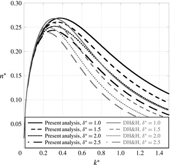
To generate an improved linear stability solution, the fourth-order ODE of Chandrasekhar, (1.5), was solved numerically using the Riccati technique with an error function mole fraction profile. The solution technique is described in appendix A. Figure 1 shows dispersion curves generated using the technique of appendix A compared with those computed using the dynamic diffusion model (1.13) of Duff et al. (Reference Duff, Harlow and Hirt1962). Figure 1 shows that the diffuse interface tends to decrease the growth rate of large-wavenumber perturbations along with the value of the most unstable wavenumber. The method of Duff et al. (Reference Duff, Harlow and Hirt1962) tends to overestimate the viscous damping of the growth rate, and underestimates the most unstable wavenumber.
A comparison of the dispersion curves generated using the diffuse-interface Rayleigh–Taylor linear stability solution developed in § 2 and appendix A (black lines), and the dynamic diffusion model (1.13) of Duff et al. (Reference Duff, Harlow and Hirt1962) (grey lines) for
 $A=0.5$
and
 $A_{{\it\mu}}=0.0$
. The two methods show different asymptotic decay behaviours, and produce different most unstable wavenumbers.

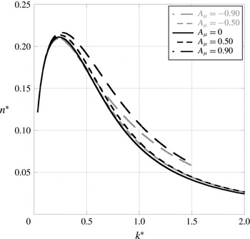
By including viscosity in the linear stability analysis, a new parameter relating to the relative strength of the two single-fluid viscosities has been added. Figure 2 shows the relatively weak effect of the viscosity contrast
 $A_{{\it\mu}}=({\it\mu}_{2}-{\it\mu}_{1})/({\it\mu}_{2}+{\it\mu}_{1})$
. Large-magnitude viscosity contrasts tend to increase the growth rates of large-wavenumber perturbations, but show a much weaker influence than the variation of Atwood number or diffusion thickness (the effect of Atwood number can be seen in figure 106 of Chandrasekhar (Reference Chandrasekhar1961), which shows an order-of-magnitude change in
 $k^{\ast }$
with an order-of-magnitude change in
 $A$
, a basic trend that is unchanged by the presence of the diffusion layer).
The effect of the viscosity contrast,
 $A_{{\it\mu}}$
, on the diffuse-interface RTI dispersion curves for
 $A=0.5$
and
 ${\it\delta}^{\ast }=5.0$
. The viscosity contrast has a weak effect on the dispersion curve, with only the largest magnitude slightly modifying the shape.

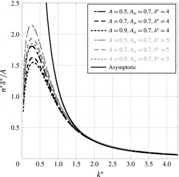
The asymptotic solution of § 3 leads to the dimensional asymptotic growth rate
 $$\begin{eqnarray}n=\frac{2Ag}{\sqrt{{\rm\pi}}{\it\nu}_{0}{\it\delta}k^{2}}.\end{eqnarray}$$
In order to test the effectiveness of the asymptotic solution, we can attempt to use it to collapse several dispersion curves in the large-wavenumber asymptotic region. Figure 3 shows the approach to the asymptotic value for several different interface thicknesses and Atwood numbers. This scaling produces a good collapse in the viscous damping region of the dispersion curves. Note that this analysis produces a
 $1/k^{2}$
asymptotic decay in growth rates and does not produce a cutoff wavenumber that results when active mass diffusion is included. However, when active diffusion is accounted for, it will result in only a small difference in the growth rate for large wavenumbers, making its effects difficult to measure. Since diffusion is not active in this analysis, we make the claim that the analysis is only valid when the growth rate
 $n$
is much larger than the diffusion time scale. That is,
 $n\gg {\it\delta}^{2}/D$
, where
 $D$
is the mass diffusion coefficient between the two fluids. Hence, this analysis may not be applicable to the far asymptotic regime where growth rates are vanishingly small, and when diffusion is strong.


5 Experimental apparatus and procedure
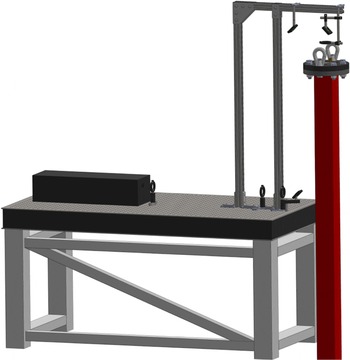
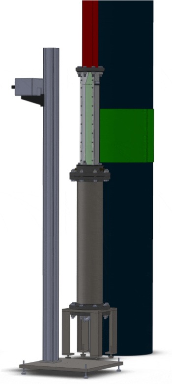
An experimental apparatus was developed to generate gas-phase RTI. Figures 4 and 5 show the three main sections of the rarefaction tube used for the current study. The bottom section is a vacuum tank that is 1.1 m long consisting of a 21.9 cm outer diameter pipe with a wall thickness of 8.2 mm. The vacuum tank is supported underneath by four steel legs, allowing access to the bottom of the tank. The bottom of the tank is enclosed by a flange with a port for the attachment of vacuum lines, and a connector for the solenoid wiring. The trigger solenoid is mounted on a beam that is suspended by two struts from the top of the vacuum tank. This beam is offset to one side to minimize the reflection of laser light into the test section above it. The solenoid structure is suspended below the test section to minimize the flow obstruction at the top of the vacuum tank.
The test section is 80.6 cm long, has an
 $88.9~\text{mm}\times 88.9~\text{mm}$
square cross-section, and is separated from the vacuum tank by the heavy-gas plenum. The heavy-gas plenum is 5.4 cm thick, and the resulting distance from the diaphragm location to the interface generation holes is 76.6 cm. The heavy-gas plenum has four 3.2 mm holes on one side to allow the heavy gas to enter. These holes minimize the amount of extra plenum gas that the rarefaction wave can draw into the test section. The test section has two 19.0 mm thick aluminium sides with an 11.2 mm thick clear acrylic front, and a black acrylic back. Each face has six small 2.3 mm holes to allow the test gases to escape and form a diffuse interface. Two PCB Piezotronics 112A21 pressure transducers are mounted on one side of the test section at 34.1 cm and 18.8 cm below the interface holes, are used to record the pressure history of the experiments, and provide trigger signals to start image acquisition. A 2.07 m long section of square fibreglass tube comprises the reflection section, resulting in a distance of 2.18 m from the interface to the top wall. This distance is long enough to prevent the transmitted rarefaction wave from reflecting and returning to the interface before the interface exits the bottom of the test section. The top of the reflection section is enclosed with a flange, where a 76 mm diameter fused silica window and two light-gas inlets are attached.
The optics used to illuminate the interface by generating a laser sheet at the top of the apparatus. The output of an Nd:YLF laser is focused, steered to the top of the apparatus, and then spread into a light sheet before entering the rarefaction tube at the top of the reflection section.

The vacuum tank, test section and the bottom of the reflection section. The interface generation holes and the laser sheet can be observed at the top of the test section. The experiments are observed by a single CMOS camera mounted to a vertical rail.

Several gas combinations were used, including CO
 $_{2}$
/SF
 $_{6}$
, air/SF
 $_{6}$
, He/CO
 $_{2}$
and He/SF
 $_{6}$
to generate a range of Atwood numbers (
 $0.4<A<0.94$
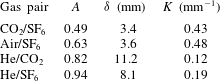
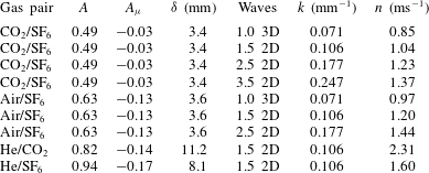
). A small amount of air was added to the heavy gas to enable smoke seeding, which slightly reduced its density. Heavy-gas densities were measured on a precise milligram balance by flowing the seeded gas through a lightweight 2 litre vessel and measuring the average weight once the balance measurement had settled. Corrected Atwood numbers are listed in table 1.
Single-mode two-dimensional (2D) perturbations are generated by rocking the apparatus side to side in the imaged plane using a method developed for single-mode shock tube experiments (Jones & Jacobs Reference Jones and Jacobs1997; Collins & Jacobs Reference Collins and Jacobs2002; Jacobs & Krivets Reference Jacobs and Krivets2005), with only the front and back interface generation holes remaining open. This motion causes 2D standing waves to form in the test section. This rocking motion is generated by an Isel Electronics
 $1.8^{\circ }/\text{step}$
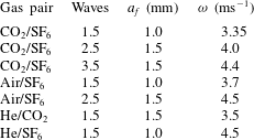
A2537-9212-A1 stepper motor that is mounted to the ceiling of the dark room in which the apparatus is located. The motor drives an eccentric cam, which is connected by an adjustable crank to the side of the tube. The phase of the forcing is measured using a small blade attached to the rotating cam that periodically interrupts an Omron EE-SPX303 optical switch. This phase information is used to determine a time delay such that the rarefaction wave arrives when the optimum interface perturbation is present. Table 2 shows the forcing frequencies, and forcing amplitudes used to generate 2D waves in the test section.
Experimentally determined gas-pair Atwood numbers and thickness parameters extracted using error function and piecewise exponential profiles. The value of
 ${\it\delta}$
is determined by the error function thickness of the interface, as in (1.11), while
 $K$
is determined from the piecewise exponential function shown in (1.8).

Forcing amplitudes
 $a_{f}$
and frequencies
 ${\it\omega}$
applied to the stepper motor and crank system to generate 2D waves in the test section.

Single-mode three-dimensional (3D) perturbations are generated by using a Tang Band W5-1138SM loudspeaker attached near the bottom of the test section to vertically oscillate the column of gas. During this oscillation, the interface generation holes on all four sides remain open. The oscillation waveform and a synchronization pulse were generated using an Agilent U2531A data acquisition board. Table 3 lists the frequencies and amplitudes applied for 3D single-mode perturbations.
Forcing frequencies
 ${\it\omega}$
and amplitudes
 $a_{f}$
applied to the loudspeaker vertical oscillation system for each of the 3D single-mode experiments.

Experiments are initiated by first flowing the light gas from the top of the apparatus, and the heavy gas from the bottom of the test section using the membraneless method of interface generation developed by Jones & Jacobs (Reference Jones and Jacobs1997). Matched volumetric flow rates of
 $6~\text{l}~\text{min}^{-1}$
are used to generate a flat diffuse interface at the location of the small holes near the top of the test section. Once this interface has stabilized, a vacuum pump begins evacuating the vacuum tank, and the pressure is monitored using an MKS-Baratron 690A53TRC pressure transducer. When the pressure drops below 0.02 atm, oscillatory forcing is initiated, and when the pressure drops below 0.01 atm, a trigger pulse synchronized with the forcing triggers a Magnetic Sensor Systems S-15-75-H solenoid to puncture a
 $23~{\rm\mu}\text{m}$
thick polypropylene diaphragm. The rupturing of the diaphragm launches a rarefaction wave upwards towards the interface, which results in a decrease in signal voltage across the two 112A21 pressure transducers. When the lower pressure transducer signal drops below
 $-0.020$
V, image acquisition is started. This voltage threshold was chosen because its magnitude is sufficiently greater than the noise threshold of the pressure transducer, but allows actuation as close in time as possible to when the rarefaction crosses the pressure transducer. Output from the pressure transducers is recorded using an Agilent U2531A data acquisition board, and images are acquired using the DaVis software from LaVision.
A Mie scattering diagnostic is employed to visualize a thin slice of the mixing region over time. Incense smoke is seeded in
 $0.6~\text{l}~\text{min}^{-1}$
of air, by passing the air through a 20 mm heat-resistant borosilicate tube containing a single incense stick. The smoke–air combination then mixes with the heavy gas flowing at
 $5.4~\text{l}~\text{min}^{-1}$
in a venturi. The downward-propagating planar laser illumination set-up is shown in figure 4. Smoke particles are illuminated by an Nd:YLF laser, which is collimated through a
 $+600~\text{mm}$
focal length lens, focused through
 $+495.7$
and
 $-495.7~\text{mm}$
focal length lenses, reflected upwards and then back downwards by three mirrors, and then formed into a sheet through a
 $-73.3~\text{mm}$
cylindrical lens. The laser sheet expands down towards the interface, illuminating it from the top. Figure 5 shows how smoke particles scatter light towards a single Photron Fastcam APX-RS CMOS camera operating at a frame rate of 12 kHz.
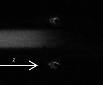
An image of an He/SF
 $_{6}$
interface visualized using Rayleigh scattered light from a single laser beam. The signal produced by this method is relatively weak, so spatial averages over multiple realizations are used.

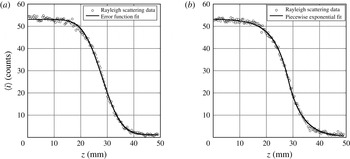
Rayleigh scattering is employed to measure the diffusion thicknesses of the initial interfaces. Unseeded test gases are used in this technique, and are illuminated by a single beam of Nd:YLF laser light at maximum power, as shown in figure 6. Light travels through the gas with negligible absorption and is scattered uniformly in all directions. The Rayleigh scattering cross-section
 ${\it\sigma}_{ray}\propto r_{p}^{6}$
, where
 $r_{p}$
is the gas particle radius (Cox, DeWeerd & Linden Reference Cox, DeWeerd and Linden2002). Therefore, the scattered light intensity is proportional to the heavy-gas concentration when the light-gas molecules are very small. Scattered light was recorded using a single CMOS camera operating at a frame rate of 60 Hz. A background image illuminating only the light gas is recorded, and then six to eight interface images with both gases are recorded. The background image is subtracted from each interface image to reduce noise. Each image is then averaged over nine pixels in the centre of the laser beam and six to eight image frames to further reduce noise. The interface thickness
 ${\it\delta}$
is obtained by fitting an error function
 $$\begin{eqnarray}h(z)=h_{0}+h_{a}\,\text{erf}\left(\frac{z-z_{0}}{{\it\delta}}\right),\end{eqnarray}$$
where
 $h$
is the scattered intensity,
 $h_{0}$
is the mean intensity,
 $h_{a}$
is intensity amplitude,
 $z$
is the vertical coordinate and
 $z_{0}$
is the coordinate of the centre of the interface.
6 Forced initial perturbations
In order to generate well-defined interface perturbations, membraneless interface generation techniques and mechanical forcing techniques were used. Figure 7 shows parameters extracted from error function, (5.1), and piecewise exponential, (1.8), fits to the Rayleigh scattering data. Good fits are observed for both profiles at all Atwood numbers; however, the error function matches the profile curvature better and approaches the limiting values more quickly. The piecewise exponential function may produce erroneous results by departing from the limiting values outside the fitted region. Extracted thickness parameters
 ${\it\delta}$
using (5.1) and
 $K$
using (1.8) are shown in table 1.
Diffusion profiles for He/SF
 $_{6}$
interfaces generated using Rayleigh scattered light. The data are curve fitted with an error function (a) and a piecewise exponential function (b). The error function appears to fit better since it has the proper asymptotic behaviour.

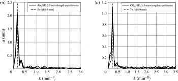
Typical spectra from (a) 2.5 wavelength experiments (air/SF
 $_{6}$
shown) and (b) 3.5 wavelength experiments (CO
 $_{2}$
/SF
 $_{6}$
shown). A strong peak is observed at the anticipated wavelength with little additional harmonic content.

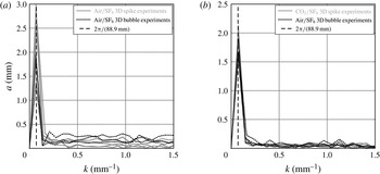
Spectra from 1.0 wavelength air/SF
 $_{6}$
(a) and CO
 $_{2}$
/SF
 $_{6}$
(b) experiments. These spectra are measured from the centre planes of 3D bubble and spike experiments. A strong peak is observed at the anticipated wavenumber with little higher harmonic content.

To characterize the quality of the single-mode perturbations, the perturbation spectra were acquired and analysed. Figure 8 shows the discrete Fourier transforms of the initial perturbations for two different sets of experiments. The spectra each show strong peaks with little harmonic content at the anticipated wavenumbers,
 $$\begin{eqnarray}k=\frac{2{\rm\pi}(m+1/2)}{88.9\;\text{mm}},\end{eqnarray}$$
where
 $m=1,2,3$
, and 88.9 mm is the width of the test section. These spectra are typical for all Atwood numbers with corresponding wavenumbers. Note that ‘single-mode’ is taken to mean that the perturbation spectrum only has a single peak, with any number of half-wavelengths present in the test section, whereas ‘1.0 wavelength’ is taken to mean that there is only a single wave crest or trough present in the test section for spike or bubble experiments, respectively. Two-dimensional perturbations are the easiest to generate for large Atwood numbers with relatively thin diffusion layers (when compared with the perturbation wavelength). However, at the largest Atwood numbers, the perturbations are difficult to form, as the required forcing frequencies become large. Additionally, it is difficult to form more than 3.5 wavelengths across the test section, as the amplitude tends to decrease near the middle of the test section, and the forcing frequency increases proportional to
 $\sqrt{k}$
.
Although we cannot presently measure the entirety of the 3D perturbations, we can partially establish their spectral content using single planar slices. Figure 9 shows the discrete Fourier transforms of the 2D slices of the initial perturbations for 3D air/SF
 $_{6}$
and CO
 $_{2}$
/SF
 $_{6}$
experiments. This 3D single-mode perturbation is of the form
 $$\begin{eqnarray}{\it\eta}(x,y)=a_{0}\cos (\tilde{k}_{x}\tilde{x})\cos (\tilde{k}_{y}{\tilde{y}}),\end{eqnarray}$$
where the
 $\tilde{x}$
and
 ${\tilde{y}}$
coordinates are along the diagonals of the test section and
 $\tilde{k}_{x}=\tilde{k}_{y}=\sqrt{2}{\rm\pi}/88.9\;\text{mm}$
, where, again, 88.9 mm is the width of the test section (Chapman & Jacobs Reference Chapman and Jacobs2006). The 3D wavenumber of the perturbation is therefore
 $$\begin{eqnarray}\sqrt{\tilde{k}_{x}^{2}+\tilde{k}_{y}^{2}}=\frac{2{\rm\pi}}{88.9\;\text{mm}},\end{eqnarray}$$
which is equivalent to the wavenumber measured from saddle point to saddle point across either the bubble or the spike.
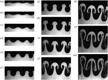
A sequence of images from a 2D CO
 $_{2}$
/SF
 $_{6}$
3.5 wavelength experiment at times (a)
 $t=0.1~\text{ms}$
, (b) 0.5 ms, (c) 0.9 ms, (d) 1.4 ms, (e) 1.8 ms, (f) 2.2 ms, (g) 2.6 ms, (h) 3.0 ms, (i) 3.4 ms, (j) 3.9 ms, (k) 4.3 ms, (l) 4.7 ms and (m) 5.0 ms. The perturbations evolve linearly in (a–d), and roll-up occurs in (e–k), with the perturbations becoming multi-valued. Finally, in panels (l) and (m) a secondary instability occurs, and the structures begin to break down.

A sequence of images from a 2D He/SF
 $_{6}$
1.5 wavelength experiment at times (a)
 $t=-0.1~\text{ms}$
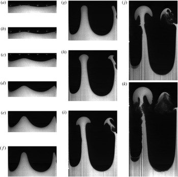
, (b) 0.3 ms, (c) 0.7 ms, (d) 1.2 ms, (e) 1.6 ms, (f) 2.0 ms, (g) 2.4 ms, (h) 2.8 ms, (i) 3.2 ms, (j) 3.7 ms and (k) 4.1 ms. Large-Atwood-number experiments exhibit strong growth that leads to a tall, round-ended spike structure, as seen in panel (g). This structure rolls up weakly as seen in panel (j), and eventually the stem of the spike breaks down in panel (k).

A sequence of images from a 3D air/SF
 $_{6}$
1.0 wavelength experiment at times (a,b)
 $t=0.0~\text{ms}$
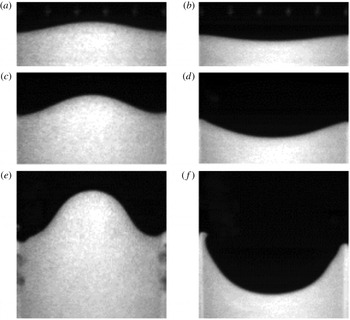
, (c,d) 1.2 ms and (e, f) 2.5 ms. The images in panels (a,c,e) are taken from an experiment in which the spike is located along the centre of the test section, while the images in panels (b,d, f) are taken from an experiment in which the bubble is located along the centre of the test section. These images show the linear growth of the 3D RTI, with panels (e, f) showing some interaction with the wall boundary layers.

7 Experimental results
Two-dimensional experiments were conducted at Atwood numbers ranging from
 $A=0.49$
to
 $A=0.94$
, with 1.5 to 3.5 wavelengths present in the test section. Figure 10 shows the evolution of short-wavelength perturbations from a low-Atwood-number,
 $A=0.49$
, CO
 $_{2}$
/SF
 $_{6}$
, 3.5 wavelength experiment, while figure 11 shows the evolution of longer-wavelength perturbations, 1.5 wavelengths, from a large-Atwood-number,
 $A=0.94$
, He/SF
 $_{6}$
experiment. The short-wavelength case in figure 10 reaches a nonlinear phase rapidly and exhibits a strong roll-up and the production of a secondary instability. The large-Atwood-number case in figure 11 produces very little roll-up initially, forming a sharp-sided round-ended spike that grows very quickly. Eventually a weak roll-up occurs, and the stem of the spike begins to diffuse away. However, both cases exhibit similar linear growth phases. Two-dimensional instability amplitude was measured by locating (by eye) the centremost bubble and spike tips, and calculating half of the vertical distance separating the two points.
Three-dimensional experiments were conducted using air/SF
 $_{6}$
and CO
 $_{2}$
/SF
 $_{6}$
. Figure 12 shows the development of the RTI from a 1.0 wavelength, 3D sinusoidal perturbation generated on an interface between air/SF
 $_{6}$
,
 $A=0.63$
. To minimize wall effects on the development of the perturbations, separate experiments were conducted to isolate the evolution of bubbles and spikes. For these 3D experiments, the bubble and spike amplitudes were extracted automatically by finding the location of the maximum gradient in a column containing the bubble and spike tips. The displacement of the flat interface was shifted in time to match the displacement of the saddle points on the wall at early times for every 3D experiment. Three-dimensional bubble and spike amplitudes could then be measured relative to the flat interface position, and the total amplitude was then taken as the average of the bubble and spike amplitudes for pairs of experiments.
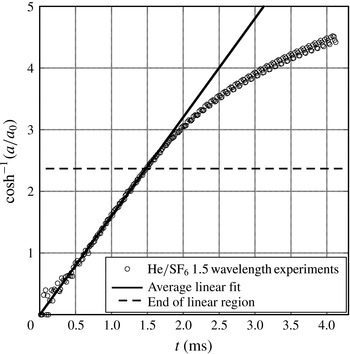
Instability growth rates were extracted from each of the single-mode experiments conducted. Figure 13 shows the measured instability amplitude from a 2D He/SF
 $_{6}$
experiment plotted using (1.4) such that growth following linear stability theory falls on a straight line. The evolution of the instability for all Atwood numbers is similar to figure 13, showing
 $\cosh (nt)$
initial growth, which decays in growth rate later in time when nonlinearity starts to influence the development. As a result, the slope of a line fitted to the linear portion of the data yields the growth rate
 $n$
. Average growth rates and parameters for each set of experiments are summarized in table 4.
The extraction of the linear growth factor from five He/SF
 $_{6}$
single-mode experiments, where
 $a$
is the amplitude of the instability and
 $a_{0}$
is the amplitude of the initial perturbation. The growth rate is found by extracting the average slope of the linear fits to
 $\text{cosh}^{-1}(a/a_{0})$
values, as justified by (1.4). The average growth rate for the He/SF
 $_{6}$
, 1.5 wavelength experiments is
 $1.60~\text{mm}^{-1}$
. Growth rates for each set of experiments are summarized in table 4. The experiments initially exhibit some variation due to the difficulty of detecting the small changes in perturbations at early time.

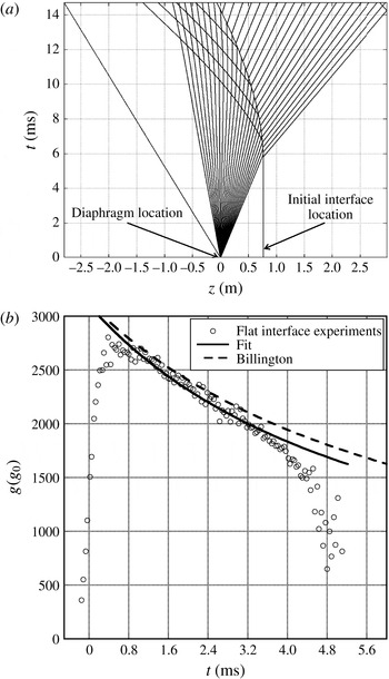
(a) The wave and interface interactions in the
 $z$
–
 $t$
plane for CO
 $_{2}$
/SF
 $_{6}$
. The refracted rarefaction wave (fanned lines) generates a sustained acceleration on the interface, and causes the interface to travel downwards. (b) The acceleration profile extracted using a moving parabolic fit to two flat-interface, CO
 $_{2}$
/SF
 $_{6}$
experiments. This profile is compared with the theory of Billington (Reference Billington1956) and a decaying power-law fit, where
 $g_{0}$
is Earth’s acceleration due to gravity.

The interaction of the rarefaction wave with the interface leads to a sustained large-magnitude acceleration. Figure 14(a) is an
 $x$
–
 $t$
diagram generated using the method of characteristics, showing the refraction of the rarefaction wave, initially shown as a rarefaction centred at the diaphragm location, while figure 14(b) shows the acceleration history produced in flat-interface experiments for the CO
 $_{2}$
/SF
 $_{6}$
cases. The refraction process results in the generation of a transmitted rarefaction wave, a reflected compression wave and the displacement of the interface down the rarefaction tube. The induced acceleration is maximum when the rarefaction wave first impacts the interface and then decays with time. Based on gas dynamic theory (Billington Reference Billington1956), this acceleration has the form
 $$\begin{eqnarray}\frac{g}{g_{max}}=\left(\frac{c_{0}t}{z_{i}}+1\right)^{-2{\it\gamma}/({\it\gamma}+1)},\end{eqnarray}$$
where
 $g_{max}$
is the peak acceleration,
 $c_{0}$
is the initial sound speed in the light gas,
 $z_{i}$
is the distance from the origin of the rarefaction wave characteristics to the initial interface location and
 ${\it\gamma}$
is the adiabatic index of the light gas. To compare with the linear stability theory described in § 2 and appendix A, which assumes a constant acceleration, an average acceleration is required. An appropriate average acceleration can be found by numerically integrating (1.3),
 $\ddot{a}(t)-kAga(t)=0$
, using the measured acceleration
 $g(t)$
, and then fitting a line to
 $\cosh ^{-1}(a/a_{0})$
versus
 $t$
to find the growth rate
 $n^{\prime }$
. The average acceleration is then taken as
 $$\begin{eqnarray}\bar{g}=\frac{(n^{\prime })^{2}}{kA}.\end{eqnarray}$$
Table 5 shows average values of acceleration extracted using (7.2). These values of acceleration vary weakly across the range of wavenumbers used (since
 $n^{\prime }$
will scale approximately as
 $\sqrt{k}$
), hence the same value of acceleration is used for all wavenumbers for a fixed Atwood number.
Extracted growth rates for three wavenumbers using CO
 $_{2}$
/SF
 $_{6}$
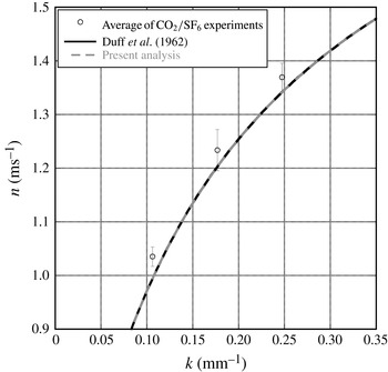
compared with diffuse-interface Rayleigh–Taylor linear stability theory (diffuse Chandrasekhar in the legend) and the inviscid result of Duff et al. (Reference Duff, Harlow and Hirt1962). The growth rates shown here are averages over four experiments, and the error bars are the 95 % confidence limits.

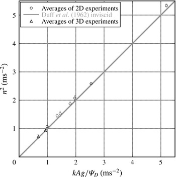
Results from single-mode experiments (
 $y$
axis) compared with the inviscid model of Duff et al. (Reference Duff, Harlow and Hirt1962) (
 $x$
axis) at all Atwood numbers. Seven sets of 2D experiments and two sets of 3D experiments are shown here. These experiments include: four experiments for CO
 $_{2}$
/SF
 $_{6}$
,
 $A=0.49$
, at 1.0 3D bubble, 1.0 3D spike, 1.5 2D, 2.5 2D and 3.5 2D wavelengths; four experiments for air/SF
 $_{6}$
,
 $A=0.63$
, at 1.0 bubble, 1.0 spike, 1.5 2D and 2.5 2D wavelengths; four experiments for He/CO
 $_{2}$
,
 $A=0.82$
, at 1.5 2D wavelengths; and five experiments for He/SF
 $_{6}$
,
 $A=0.94$
, at 1.5 2D wavelengths. The growth rates shown here are averages over four experiments (five for He/SF
 $_{6}$
), and the error bars are the 95 % confidence limits.

A summary of the basic parameters and measured average growth rates for the experiments presented here. The Atwood number was adjusted to account for the dilution of the heavy gas by smoke and air from the tracer seeding process. The parameter
 ${\it\delta}$
was measured using a Rayleigh scattering technique, and
 $k$
was measured using the initial images of the interface prior to acceleration. The growth rate is found by extracting the average slope of the linear fits to
 $\text{cosh}^{-1}(a/a_{0})$
values as in figure 13. Values of
 $A_{{\it\mu}}$
were determined from the pure fluid values of viscosity (no seeding) using the software REFPROP at 23.6
 $^{\circ }$
C (Lemmon, Huber & McLinden Reference Lemmon, Huber and McLinden2013).

Weighted average accelerations during the linear growth phase, where
 $g_{0}$
is Earth’s acceleration due to gravity. These weighted accelerations are extracted numerically using (7.2).

To assess the quality of the theoretically generated dispersion curves, they were compared with experimentally extracted wavenumbers and growth rates. Figure 15 shows the extracted growth rates obtained from 2D CO
 $_{2}$
/SF
 $_{6}$
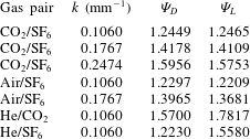
experiments taken at three different wavenumbers, compared with dispersion curves generated using the inviscid method of Duff et al. (Reference Duff, Harlow and Hirt1962) (similar to (1.9)), and the computed growth rates of the stability analysis described in § 2 and appendix A. Table 6 shows the values of
 ${\it\Psi}$
used in (1.9) calculated for all of the experimental cases. By using the averaged acceleration
 $\bar{g}$
, the experimental points in figure 15 exhibit good agreement with the diffuse-interface, linear stability theory. It can also be seen, for these relatively inviscid experiments, that the inviscid model of Duff et al. (Reference Duff, Harlow and Hirt1962) agrees well with the complete viscous solution. Therefore, the inviscid method of Duff et al. (Reference Duff, Harlow and Hirt1962) can be seen as the inviscid limit of the exact solution. Figure 16 shows growth rates from all of the experiments presented herein compared with the inviscid model of Duff et al. (Reference Duff, Harlow and Hirt1962). The experiments agree well with the theory, but the 2D experimental measurements are consistently slightly larger. This slight disagreement may be due to weak three-dimensionality increasing the effective wavelength. It should be noted that the application of the model of Weber, Cook & Bonazza (Reference Weber, Cook and Bonazza2013) in which the vorticity is integrated would probably yield an improvement in these initial growth estimates. The 3D experiments show better agreement, and represent the most inviscid perturbations due to their large wavelengths.
Growth reduction factors extracted using the methods of LeLevier et al. (Reference LeLevier, Lasher and Bjorklund1955) and Duff et al. (Reference Duff, Harlow and Hirt1962). These factors reduce the growth of the instability in the manner described by (1.9), and are generated based on data extracted using fits to Rayleigh scattering data.

8 Conclusions
Theory and experiments have been reported that explore the behaviour of the RTI initiated with a diffuse interface. When RTI is initiated with a diffuse interface, the growth rate of the instability is decreased. The Duff et al. (Reference Duff, Harlow and Hirt1962) dynamic diffusion model disagrees with the complete viscous diffuse-interface linear stability theory in § 2 and appendix A in the large-wavenumber regime where the complete solution predicts larger growth rates and a larger most unstable wavenumber. The asymptotic analysis of § 3 shows a
 $1/k^{2}$
decay in the growth rate at large wavenumbers. This decay makes it very difficult to observe growth for large wavenumbers as they will require long development times. Experiments that observe growth from short-wavelength perturbations would be useful to test the effectiveness of the linear stability analyses where viscosity is important, and where the theory of Duff et al. (Reference Duff, Harlow and Hirt1962) is most approximate. However, owing to the difficulties in generating this class of perturbations, they were unable to be tested herein.
The experiments presented here improve upon the previous gas-phase single-mode experiments of Duff et al. (Reference Duff, Harlow and Hirt1962) by initiating the RTI with well-defined sinusoidal perturbations. These experiments use a rarefaction wave to generate a large, non-constant acceleration on an interface between two gases. This large acceleration puts these experiments in a regime that starts to bridge the gap between classical RTI experiments and laser-driven RTI experiments. Nine sets of experiments were presented with Atwood numbers ranging from
 $A=0.49$
to 0.94, and wavenumbers ranging from
 $k=0.0707$
to
 $0.2474~\text{mm}^{-1}$
. These experiments show that variable acceleration has little effect on the early stage of the RTI, if accounted for by a weighted average of the variable acceleration. Since these experiments are relatively inviscid, the growth reduction factor given by Duff et al. (Reference Duff, Harlow and Hirt1962) predicts the decrease in the growth rate due to an initially diffuse interface. Finally, this experiment exhibits a new method for generating gas-phase RTI at large Atwood numbers in the range
 $0.5<A<1$
.
Appendix A. Numerical solution of the generalized linear stability equation
Equation (1.5) for a system of superposed fluids with a spatially varying density and viscosity is solved numerically by the Riccati method. The Riccati transformation is given in detail by Scott (Reference Scott1973) and has been used in numerous stability analyses (Drazin & Reid Reference Drazin and Reid1981). Introduction of the function
 ${\it\chi}={\it\psi}^{\prime \prime }-{k^{\ast }}^{2}{\it\psi}$
allows one to reduce (2.2) to the form
 $$\begin{eqnarray}\displaystyle & & \displaystyle \frac{\text{d}}{\text{d}{\it\zeta}}\left[{\it\rho}^{\ast }{\it\psi}^{\prime }-\frac{{\it\mu}^{\ast }}{n^{\ast }}{\it\chi}^{\prime }-\frac{1}{n^{\ast }}{{\it\mu}^{\ast }}^{\prime }{\it\chi}-\frac{2{k^{\ast }}^{2}}{n^{\ast }}{{\it\mu}^{\ast }}^{\prime }{\it\psi}\right]\nonumber\\ \displaystyle & & \displaystyle \quad ={k^{\ast }}^{2}\left[-\frac{1}{{n^{\ast }}^{2}}{{\it\rho}^{\ast }}^{\prime }{\it\psi}+{\it\rho}^{\ast }{\it\psi}-\frac{{\it\mu}^{\ast }}{n^{\ast }}{\it\chi}-\frac{2}{n^{\ast }}{{\it\mu}^{\ast }}^{\prime }{\it\psi}^{\prime }\right].\end{eqnarray}$$
By introducing two vector functions
 $$\begin{eqnarray}\hat{\boldsymbol{u}}=\left(\begin{array}{@{}c@{}}{\it\psi}^{\prime }\\ {\it\chi}^{\prime }\end{array}\right)\quad \text{and}\quad \hat{\boldsymbol{v}}=\left(\begin{array}{@{}c@{}}{\it\psi}\\ {\it\chi}\end{array}\right),\end{eqnarray}$$
(A 1) can be written as
 $$\begin{eqnarray}\hat{\boldsymbol{u}}^{\prime }=\left(\begin{array}{@{}c@{}}{\it\psi}^{\prime \prime }\\ {\it\chi}^{\prime \prime }\end{array}\right)=\unicode[STIX]{x1D63C}\left(\begin{array}{@{}c@{}}{\it\psi}^{\prime }\\ {\it\chi}^{\prime }\end{array}\right)+\unicode[STIX]{x1D63D}\left(\begin{array}{@{}c@{}}{\it\psi}\\ {\it\chi}\end{array}\right),\end{eqnarray}$$
where
 $\unicode[STIX]{x1D63C}$
and
 $\unicode[STIX]{x1D63D}$
are matrices of the form
 $$\begin{eqnarray}\unicode[STIX]{x1D63C}=\left[\begin{array}{@{}cc@{}}0 & 0\\ \displaystyle n^{\ast }\frac{{\it\rho}^{\ast \prime }}{{\it\mu}^{\ast }} & \displaystyle -2\frac{{\it\mu}^{\ast \prime }}{{\it\mu}^{\ast }}\end{array}\right]\end{eqnarray}$$
and
 $$\begin{eqnarray}\unicode[STIX]{x1D63D}=\left[\begin{array}{@{}cc@{}}{k^{\ast }}^{2} & 1\\ \displaystyle -2{k^{\ast }}^{2}\frac{{\it\mu}^{\ast \prime \prime }}{{\it\mu}^{\ast }}+\frac{{k^{\ast }}^{2}}{n^{\ast }}\frac{{\it\rho}^{\ast \prime }}{{\it\mu}^{\ast }} & \displaystyle n^{\ast }\frac{{\it\rho}^{\ast }}{{\it\mu}^{\ast }}-\frac{{\it\mu}^{\ast \prime \prime }}{{\it\mu}^{\ast }}+{k^{\ast }}^{2}\end{array}\right].\end{eqnarray}$$
Then the Riccati matrix
 $\unicode[STIX]{x1D64D}$
is introduced with the transformation
 $$\begin{eqnarray}\hat{\boldsymbol{u}}=\unicode[STIX]{x1D64D}\hat{\boldsymbol{v}}.\end{eqnarray}$$
Differentiating this equation,
 $$\begin{eqnarray}\hat{\boldsymbol{u}}^{\prime }=\unicode[STIX]{x1D64D}^{\prime }\hat{\boldsymbol{v}}+\unicode[STIX]{x1D64D}\hat{\boldsymbol{v}}^{\prime },\end{eqnarray}$$
and using (A 3), it follows that
 $\unicode[STIX]{x1D64D}$
satisfies the nonlinear matrix differential equation
 $$\begin{eqnarray}\unicode[STIX]{x1D64D}^{\prime }=\unicode[STIX]{x1D63C}\unicode[STIX]{x1D64D}+\unicode[STIX]{x1D63D}-\unicode[STIX]{x1D64D}\unicode[STIX]{x1D64D}.\end{eqnarray}$$
To formulate the eigenvalue problem it is necessary to impose boundary conditions at
 ${\it\zeta}\rightarrow \pm \infty$
. Considering asymptotic solutions of (A 1) far from the interface, when
 ${\it\zeta}\rightarrow \pm \infty$
, the differential equation reduces to
 $$\begin{eqnarray}{\it\psi}^{\prime \prime }-\frac{{\it\nu}^{\ast }}{n^{\ast }}({\it\psi}^{\text{IV}}-{k^{\ast }}^{2}{\it\psi}^{\prime \prime })={k^{\ast }}^{2}{\it\psi}-{k^{\ast }}^{2}\frac{{\it\nu}^{\ast }}{n^{\ast }}({\it\psi}^{\prime \prime }-{k^{\ast }}^{2}{\it\psi}),\end{eqnarray}$$
where
 ${\it\nu}^{\ast }={\it\mu}^{\ast }/{\it\rho}^{\ast }$
. For
 ${\it\zeta}\rightarrow -\infty$
, (A 9) has the solution
 $$\begin{eqnarray}{\it\psi}=A_{1}\text{e}^{k^{\ast }{\it\zeta}}+B_{1}\text{e}^{q^{\ast }{\it\zeta}},\end{eqnarray}$$
where
 $q^{\ast }=\sqrt{{k^{\ast }}^{2}+n^{\ast }/{\it\nu}^{\ast }}$
(note that
 ${\it\nu}^{\ast }$
and
 $q^{\ast }$
will take different values on each side of the interface). Combining the first and third derivatives, one obtains the following expressions:
 $$\begin{eqnarray}{\it\psi}^{\prime \prime \prime }-{k^{\ast }}^{2}{\it\psi}^{\prime }=q^{\ast }({\it\psi}^{\prime \prime }-{k^{\ast }}^{2}{\it\psi}),\end{eqnarray}$$
and
 $$\begin{eqnarray}{\it\psi}^{\prime \prime \prime }-{q^{\ast }}^{2}{\it\psi}^{\prime }=k^{\ast }({\it\psi}^{\prime \prime }-{q^{\ast }}^{2}{\it\psi}).\end{eqnarray}$$
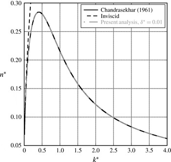
A comparison of the numerical solution of appendix A, the viscous sharp-interface result of Chandrasekhar (Reference Chandrasekhar1961) from (1.5), and the inviscid solution of (1.1) for
 $A=0.5$
and
 $A_{{\it\mu}}=0.5$
. Good agreement is found at all wavenumbers for sufficiently small choices of
 ${\it\delta}^{\ast }$
.

Then substituting
 ${\it\chi}={\it\psi}^{\prime \prime }-{k^{\ast }}^{2}{\it\psi}$
, subtracting (A 12) from (A 11), and making use of
 ${\it\chi}^{\prime }=q^{\ast }{\it\chi}$
, the relationship
 $$\begin{eqnarray}({q^{\ast }}^{2}-{k^{\ast }}^{2}){\it\psi}^{\prime }=q^{\ast }{\it\chi}-k^{\ast }{\it\psi}^{\prime \prime }+k^{\ast }{q^{\ast }}^{2}{\it\psi}\end{eqnarray}$$
is obtained. Upon addition and subtraction of
 ${k^{\ast }}^{3}{\it\psi}$
to the right-hand side, (A 13) reduces to
 $$\begin{eqnarray}\displaystyle {\it\psi}^{\prime }=\frac{1}{(q^{\ast }+k^{\ast })}{\it\chi}+k^{\ast }{\it\psi}. & & \displaystyle\end{eqnarray}$$
Finally, the boundary condition for the Riccati matrix
 $\unicode[STIX]{x1D64D}$
at
 ${\it\zeta}\rightarrow -\infty$
assumes the form
 $$\begin{eqnarray}\unicode[STIX]{x1D64D}(z\rightarrow -\infty )\hat{\boldsymbol{v}}=\hat{\boldsymbol{u}}=\left(\begin{array}{@{}c@{}}{\it\psi}^{\prime }\\ {\it\chi}^{\prime }\end{array}\right)=\left(\!\begin{array}{@{}cc@{}}k^{\ast } & (q^{\ast }+k^{\ast })^{-1}\\ 0 & q^{\ast }\end{array}\!\right)\left(\begin{array}{@{}c@{}}{\it\psi}\\ {\it\chi}\end{array}\right),\end{eqnarray}$$
since
 ${\it\chi}^{\prime }=q^{\ast }{\it\chi}$
. Applying a similar derivation at
 ${\it\zeta}\rightarrow \infty$
, the boundary condition for the Riccati matrix yields the expression
 $$\begin{eqnarray}\unicode[STIX]{x1D64D}(z\rightarrow \infty )\hat{\boldsymbol{v}}=\hat{\boldsymbol{u}}=\left(\begin{array}{@{}c@{}}{\it\psi}^{\prime }\\ {\it\chi}^{\prime }\end{array}\right)=\left(\begin{array}{@{}cc@{}}-k^{\ast } & -(q^{\ast }+k^{\ast })^{-1}\\ 0 & -q^{\ast }\end{array}\!\right)\left(\begin{array}{@{}c@{}}{\it\psi}\\ {\it\chi}\end{array}\right).\end{eqnarray}$$
Note that the non-dimensional kinematic viscosity, according to (2.8) and (2.9), is expressed as
 $$\begin{eqnarray}{\it\nu}_{\pm }^{\ast }=\frac{1\mp A_{{\it\mu}}}{1\mp A}.\end{eqnarray}$$
In order to solve the eigenvalue problem numerically for
 $$\begin{eqnarray}n^{\ast }=n^{\ast }(k^{\ast },{\it\delta}^{\ast },A_{{\it\mu}},A),\end{eqnarray}$$
(1.1) is solved for the sharp density profile in the inviscid limit to obtain an estimate for
 $n_{inv}^{\ast }=\sqrt{k^{\ast }A}$
. This value of
 $n_{inv}^{\ast }$
is used as an initial guess in an iteration process to find
 $n^{\ast }$
from the viscous solution with the additional parameters
 ${\it\delta}^{\ast }$
and
 $A_{{\it\mu}}$
. By progressing to increasing wavenumbers from the inviscid (small-wavenumber) limit, the required growth rate can be found. In this procedure, the initial value problem (A 8) is solved using a fourth-order Runge–Kutta numerical integration. The solution is generated from the positive and negative
 ${\it\zeta}$
sides with appropriate boundary conditions, (A 15) and (A 16), thus obtaining two Riccati matrices
 $\unicode[STIX]{x1D64D}^{+}$
and
 $\unicode[STIX]{x1D64D}^{-}$
as a function of
 ${\it\zeta}$
. The eigenvalue parameter is varied using a secant method until the residual
 $$\begin{eqnarray}{\it\epsilon}=\det |\unicode[STIX]{x1D64D}^{+}(0)-\unicode[STIX]{x1D64D}^{-}(0)|\end{eqnarray}$$
satisfies
 ${\it\epsilon}<1\times 10^{-6}$
, ensuring that the solution is continuous through
 ${\it\zeta}=0$
. Figure 17 shows a comparison of the method developed in this section with the sharp interface method of Chandrasekhar. Good agreement is observed for vanishing interface thickness,
 ${\it\delta}^{\ast }$
.