





1. Introduction
The Epoch of Reionisation (EoR) marks the period during which the intergalactic medium (IGM) transitioned from predominantly neutral to ionised. Constraining the timescale and drivers of this process requires characterising the sources of ionising photons to constrain their possible contributions, even though direct detection of Lyman-continuum (LyC) emission is prevented by the opacity of the early IGM (Robertson et al. Reference Robertson, Ellis, Dunlop, McLure and Stark2010a,b). It is yet unclear if the major contributors to reionisation were massive bright galaxies (Sharma et al. Reference Sharma, Theuns and Frenk2018; Naidu et al. Reference Naidu, Tacchella, Mason, Bose, Oesch and Conroy2020) or more numerous faint ones (
 $M_{UV}\gt -18$
) (Ciardi et al. Reference Ciardi, Ferrara and White2003; Bouwens et al. Reference Bouwens2012; Robertson et al. Reference Robertson, Ellis, Dunlop, McLure and Stark2010a).
Since the launch of JWST, the ionising photon production efficiency parameter,
 $\mathrm{\xi_{ion}}$
, has become a central tool for quantifying the LyC contribution of galaxies to reionisation. It has been measured for direct EoR sources (Simmonds et al. Reference Simmonds2023; Boyett et al. Reference Boyett2024; Pahl et al. 2025; Harshan et al. Reference Harshan2024; Papovich et al. Reference Papovich2026), for EoR analogues at intermediate (Tang et al. Reference Tang, Stark, Chevallard and Charlot2019; Jaiswar et al. Reference Jaiswar, Gupta, da Cunha, Trott, Harshan, Battisti and Forrest2024) and low (Cardamone et al. Reference Cardamone2009; Izotov et al. 2018) redshifts and for specially selected sources (Stark et al. Reference Stark2014; Gupta et al. 2023).
Low-mass or ‘faint’ galaxies remain compelling candidates for driving reionisation due to their early formation, high number densities (thus large UV luminosity density
 $\rho_{UV}$
) (Balu et al. Reference Balu, Greig, Qiu, Power, Qin, Mutch and Wyithe2023; Cook et al. Reference Cook, Balu, Greig, Trott, Line, Qin and Wyithe2024), elevated specific SFRs at high redshift (
 $z\gt 6$
) (Robertson et al. Reference Robertson2023) in comparison to the low redshift equivalents, and the potential for shallower gravitational wells that promote LyC escape via stellar wind and radiation driven feedback (Izotov et al. 2018; Finkelstein et al. Reference Finkelstein2019). The Ly
 $\alpha$
forest exhibited by quasars in the EoR has always suggested a significant density of neutral Hydrogen (HI) gas toward the recent end of the EoR, which is better modelled by low-mass contributors (Kulkarni et al. Reference Kulkarni, Keating, Haehnelt, Bosman, Puchwein, Chardin and Aubert2019).
However, the tendency to select interesting sources to analyse can lead to biases in our understanding of ionising emission properties. Galaxies exhibiting bright emission lines (Bunker et al. Reference Bunker2023; Carniani et al. Reference Carniani2024; Helton et al. Reference Helton2024), lacking dust obscuration (Jaiswar et al. Reference Jaiswar, Gupta, da Cunha, Trott, Harshan, Battisti and Forrest2024; Setton et al. Reference Setton2025), having atypical continuum profiles (Cameron et al. Reference Cameron, Katz, Witten, Saxena, Laporte and Bunker2024), or those interacting with other galaxies (Gupta et al. Reference Helton2023; Mascia et al. Reference Mascia2025) may not represent the general population but are over-represented in this field of study. Such samples are highly informative, but may not represent the underlying population, and analyses that rely exclusively on them risk biasing the inferred ionising budgets and obscuring the true evolution of ionising parameters (Simmonds et al. Reference Simmonds2024).
Large direct studies of faint, high-redshift (
 $M_{UV}\gt -18, z\gt 6$
) sources with good constraints are scarce (Harshan et al. Reference Harshan2024) and creating a true analogue sample at lower redshifts without a proper calibration sample is difficult because of this. However, constraining the relationship of probes for the escape fraction of LyC photons (
 $\,f_{\rm esc}$
) and
 $\mathrm{\xi_{ion}}$
with these parameters is becoming more accessible with the depth of new programs.
In this paper we present a new sample from the OutThere survey, a wide-area pure-parallel spectroscopic James Webb Space Telescope (JWST) program. Our selection identifies
 $z\sim2$
[OIII]5007 and H
 $\alpha$
emitters across the full range of detected equivalent widths, enabling us to probe the low-EW and low-ionising-efficiency regimes that are typically inaccessible or unreported in similar high-redshift studies. The aim of this work is to construct a large, low–entry-barrier control sample at intermediate redshift (
 $z\sim2$
) that can serve as a baseline for interpreting bright and faint emission-line populations observed deep into the EoR. The optical coverage and high-quality photometry available at these redshifts allow us to constrain stellar and ionising properties more reliably than is possible for
 $z\gt 6$
systems, providing a reference against which EoR measurements can be placed in context. We note that, because spectroscopic redshifts require identifiable emission features, the sample necessarily favours galaxies with detected [OIII]5007 and H
 $\alpha$
; however, within this constraint we include the full observed range of line strengths to minimise additional selection bias.
2. Data and methods
The rate of ionisation N
 $_{\rm ion}$
at some given epoch is parameterised by the fraction of escaping Lyman Continuum light (
 $\,{f_{\rm esc}}$
), the ionising photon production efficiency (
 $\mathrm{\xi_{ion}}$
) and the number density of ionising sources within a co-moving volume,
 $\rho_{UV}$
(Robertson et al. Reference Robertson, Ellis, Dunlop, McLure and Stark2010a). Here we explain our derivation of the
 ${f_{\rm esc}}$
and
 $\mathrm{\xi_{ion}}$
parameters that are used in this work. We also explore the OutThere spectroscopic survey data and the combined photometric catalogues used to derive these parameters.
2.1. OutThere survey
The OutThere survey is a JWST pure-parallel program using the Near Infrared Imager and Slitless Spectrograph (NIRISS) instrument grism spectroscopy. As of writing, this survey has collected data from 120/127 expected fields over 425 h, making it the largest such JWST program to date. This work focuses on a selection of 12 pointings over 48 sq.arcmin in the Hubble Ultra-Deep Field-North (HUDF-N) field. We use the F150W and F200W filters which give the reddest spectra up to 2.2
 $\unicode{x03BC}$
m with a depth of more than 12.5 h. JWST OutThere is associated with JWST PID 3383 and PID 4681. Data used here can be found using MAST DOI: 10.17909/e3be-gp53.
2.2. Photometry and selection
To constrain the physical and selection parameters of these galaxies, we use the combined photometric data publicly available from the JADES (Eisenstein et al. Reference Eisenstein2025), PANORAMIC (Williams et al. Reference Williams2021), CONGRESS (Egami et al. Reference Egami2023) and SAPPHIRES (Egami et al. Reference Egami2024) programs in the HUDF-N field. This internal, multi-band catalogue was constructed using JWST NIRISS, Hubble Space Telescope (HST) ACS/WFC and JWST Near Infrared Camera (NIRCam) Grizli-reduced imaging from these programs spanning 24 filters from F435W to F460M.
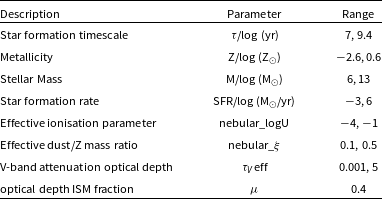
Prior ranges set for each parameter in the BEAGLE SED model. All ranges use uniform distributions.

Table 1. Long description
A table with two columns and nine rows. The first column is labeled ‘Description’ and the second column is labeled ‘Parameter’ and ‘Range’. The table lists the following data: Row 1: Star formation timescale, /log (yr), 7, 9.4. Row 2: Metallicity, Z/log (Z), , 0.6. Row 3: Stellar Mass, M/log (M), 6, 13. Row 4: Star formation rate, SFR/log (M/yr), , 6. Row 5: Effective ionisation parameter, nebular_logU, , . Row 6: Effective dust/Z mass ratio, nebular_, 0.1, 0.5. Row 7: V-band attenuation optical depth, , 0.001, 5. Row 8: optical depth ISM fraction, , , 0.4.
Galaxies were selected to contain detected [OIII]5007 and H
 $\alpha$
emission lines between
 $1.6\lt z\lt 2.5$
as well as at least 12/24 filters in order to consider only well sampled spectral energy distributions (SEDs) and so that the filters captured both lines. This provides an initial sample of 371 sources. Adding a SN
 $\gt 3$
cut on H
 $\alpha$
reduces this sample to 277. We found 3 out of our 277 galaxies did not converge on a solution from SED fitting with the priors (see Table 1) used by the full sample. To maintain consistent working priors across the entire sample, these were removed. A further 41 galaxies were eliminated due to poorly reduced spectra as detailed in Section 2.3 (see Figures 1 and 2), giving a sample of 233 galaxies. Figure 3 shows some general properties (SFH, dust/age correlation) and diagnostics regarding the SED modelling.
This photometry was fitted using the BEAGLE SED fitting code (Chevallard & Charlot Reference Chevallard and Charlot2016; Gutkin et al. Reference Gutkin, Charlot and Bruzual2016), a Bayesian tool which interprets the physical parameters of the galaxy from this fit. It contains the BC16 SPS model, which is an updated version of Bruzual & Charlot (Reference Bruzual and Charlot2003), CLOUDY photo-ionisation (Ferland et al. Reference Ferland2017), CF00 dust model (Charlot & Fall Reference Charlot and Fall2000), delayed-tau star formation history and a free parameter constant SFH at 10 Myr. BEAGLE self consistently considers dust within the nebular emission model when using two component dust models (such as CF00) hence our choice of model.
We determine the quality of these fits using the reduced
 $\chi^2$
and remove sources above
 $\chi^2=3.5$
or which had
 $\chi^2=0$
(3 sources). This sets the final sample as 230 galaxies. The fitting uses the prior ranges in Table 1.
2.3. OutThere spectroscopy
At the time of publication the OutThere survey is limited to its internal data releases. Data processing and calibration are still in progress, particularly relating to the trace and wavelength calibrations. Spectral extraction and emission line measurements are affected by NIRISS contamination and should be interpreted with appropriate caution. Full descriptions of the reduction, calibration steps, and sensitivities will be presented in forthcoming OutThere papers once the pipeline is stabilised. As a result, we visually classify individual sources to eliminate failed emission line fits, bad redshift constraints and poorly modelled contamination. This process eliminated 41/274 sources.
The visual classification was performed by grouping galaxies into ‘good’ and ‘bad’ examples of forward-modelled, slitless NIRISS data, where the borderline galaxies were grouped into either category. The visual selection criteria of good and borderline-good sources are exemplified in Figure 1 while Figure 2 exemplifies borderline-bad and bad sources from top to bottom. Figure 1 (top) shows an ideal fit, where the Grizli pipeline has modelled both the contamination and the continuum before calculating the identified emission lines, and the redshift fit is of high certainty. The bottom panel shows an example of a source accepted despite contamination and residual continuum being clearly visible in the final 2D spectrum. As the contamination is spatially distinct in the 2D spectrum from the emission lines of interest, and as the redshift certainty appears significant, this galaxy was also included in the final sample. Figure 2 (top) shows an example source with significant contamination in both F150W and F200W. While the model appears to eliminate this contamination and the underlying continuum, this source appears to derive its H
 $\alpha$
flux from an elongated feature that is present in its contamination model which has not been properly masked. To ensure the purity of the H
 $\alpha$
flux in our sample, this source was eliminated. The bottom panel shows a source with poorly modelled contamination that is not distinct from the galaxy and appears on the edge of the filter. Furthermore, it has multiple likely redshift solutions and so was rejected from the final sample.
2.4. Dust correcting H
 $\alpha$

At the spectral resolution of our NIRISS spectra, H
 $\alpha$
(6 563 Å) is blended with the double peaked [NII] (6 548, 6 583), which would overestimate its flux (Faisst et al. Reference Faisst, Masters, Wang, Merson, Capak, Malhotra and Rhoads2018). We utilise the photo-ionisation modelling of our SEDs to proportionally subtract these emission line fluxes from the H
 $\alpha$
flux as:
 \begin{equation} \mathrm{F_{H\alpha-NII} = F_{H\alpha}^{spec} \times \left(1- \frac{F_{[NII]_{6\,548}^{Model}}+F_{[NII]_{6\,583}^{Model}}}{F_{{H\alpha}^{Model}}}\right)}\end{equation}
We then correct the H
 $\alpha$
emission for dust absorption by considering the CF00 attenuation model using the BEAGLE SED derived
 $A_V$
value as:
 \begin{equation} \begin{split} {\tau_V = \frac{A_V}{1.086 \times 0.44}}, \\[3pt] {k_{{\rm H}\alpha} = \left(\frac{6563}{5500}\right)^{-1.3}},\\[3pt] {{\rm H}\alpha_{\rm int}={\rm H}\alpha \times 10^{(0.4 \times \tau_V \times k_{{\rm H}\alpha})}}, \end{split}\end{equation}
which uses the reference wavelength of 5 500 Å and the birth cloud (BC) absorption coefficient of
 $n=1.3$
from the CF00 dust attenuation model. We use the factor of 0.44 to convert from stellar to nebular
 $A_V$
(Calzetti et al. Reference Calzetti, Armus, Bohlin, Kinney, Koornneef and Storchi-Bergmann2000; Battisti et al. Reference Battisti, Calzetti and Chary2016). All reported H
 $\alpha$
refers to this dust corrected version. Figure 3’s top left panel shows the BEAGLE derived
 $A_V$
distribution for this sample (1
 $\sigma$
 $A_V = 0.14^{+0.37}_{-0.11}$
). It is worth noting the dependence of these results on the exact implementation of dust corrections, which were not explored in this work. Applying a stronger dust attenuation factor makes many of the noted relations correlate where they previously did not, as the most dusty galaxies are very dependent on this factor. An unorthodox method to correct for dust was explored using the BEAGLE model, such that the modelled emitted and observed H
 $\alpha$
correct the spectroscopic H
 $\alpha$
as:
 \begin{equation} \mathrm{ H\alpha^{corr} = H\alpha^{spec} \times \frac{H\alpha^{em}}{H\alpha^{obs}}},\end{equation}
though ultimately this was deemed to introduce too large a model dependence. Alternatively, an argument could be made for the factor
 $n=1.3$
in the calculation of
 $\tau_{{\rm H}\alpha}$
to instead be
 $n=0.7$
for the diffuse ISM attenuation following the birth cloud. Yet additionally, the factor of 0.44 used to convert the stellar
 $A_V$
to a nebular value is not well supported (Reddy et al. Reference Reddy2015). These uncertainties in the method should be noted and revisited with a deeper understanding of the underlying processes causing them.
Sample 1D and 2D spectra in both F150W and F200W and redshift likelihood fit for galaxy 6338 (top) and 13736 (bottom), with highly certain z fits and well isolated emission lines. 6338 is given as an ideal example of the Grizli reduction pipeline while 13736 is given as a reasonably well fit example where the remaining contamination does not overlap spatially with our source. These are included in the final sample.

Sample 1D and 2D spectra in both F150W and F200W and redshift likelihood fit for galaxy 12110 (top) and 18393 (bottom). 12110 is given as a borderline example of the of the Grizli reduction pipeline while 18393 is given as a poorly constrained example. 12110 is considered borderline as while the z fit is certain it appears to derive the H
 $\alpha$
emission line from a feature that is present in the contamination model. 18393 is considered a failed fit as the H
 $\alpha$
line falls on the filter edge and has two major z fit peaks. These are not included in the final sample.

Quality control and diagnostic tests for our 230 OutThere galaxy sample. (a) (Left) Dust attenuation per galaxy count determined using BEAGLE and the CF00 dust law. (Right) Relative difference of the modelled H
 $\alpha$
emission line flux to the OutThere NIRISS H
 $\alpha$
flux (orange) over-plotted with the separation of the modelled SED to the photometry (purple, reduced
 $\chi^2$
). (b) (Left) UV slope correlation with stellar ages and dust attenuation. (Right) Star formation history averages over 5 bins of
 $\mathrm{\xi_{ion}^{HII}}$
. We find that most of our BEAGLE SED galaxies experience low dust attenuation and underestimate the H
 $\alpha$
flux. The UV slope is more strongly related to the dust attenuation than to the stellar age. We find no clear starburst behaviour responsible for particularly high
 $\mathrm{\xi_{ion}^{HII}}$
.

2.5. Determining
$\boldsymbol{\xi}_{\mathrm{ion}}$

The ionising photon production efficiency quantifies the intrinsic production rate of hydrogen-ionising photons relative to the non-ionising UV continuum luminosity, which traces the young stellar population. The primary derivation method of
 $\mathrm{\xi_{ion}}$
using H
 $\alpha$
emission (hence
 $\mathrm{\xi_{ion}^{HII}}$
) (Simmonds et al. Reference Simmonds2023) follows:
 \begin{equation} \begin{split} N(H^0) = L({\rm H}\alpha)\times7.28\times10^{11}, \\[3pt] \log_{10}(\xi_{\rm ion}^{HII})=\log_{10}\left(\frac{N(H^0)}{L_{UV}}\right) \end{split}\end{equation}
where
 $N(H^0)$
is the total rate of hydrogen-ionising photons (s
 $^{-1}$
) produced, L(H
 $\alpha$
) is the H
 $\alpha$
luminosity (in erg s
 $^{-1}$
), and
 $L_{UV}$
is the intrinsic (dust-corrected) non-ionising UV luminosity (in erg s
 $^{-1}$
Hz
 $^{-1}$
), typically measured at 1 500 Å as we have done.
This follows the assumption that most of the ionising emissions from massive stars is absorbed by their birth cloud nebulae, emitting a significant amount of H
 $\alpha$
among other common lines. This also assumes that no LyC escapes the nebula.
2.6. Determining
${\boldsymbol{f}_{\rm esc}}$

Without an intrinsic understanding of the LyC photons produced and a direct measure of the escaping portion, determining
 ${f_{\rm esc}}$
comes down to empirical probes determined at low redshift (Izotov et al. 2018; Izotov et al. Reference Izotov, Chisholm, Worseck, Guseva, Schaerer and Prochaska2022). Applying these to higher redshift galaxies is scientifically ambiguous, as the environments from which the LyC escapes are distinct in more evolved systems (see ionisation vs density bounded nebula discussion in Zackrisson et al. Reference Zackrisson, Inoue and Jensen2013 for an explanation of the screen and hole models). Using the relation from Chisholm et al. (Reference Chisholm2022):
 \begin{equation} f_{\rm esc} = (1.3 \pm 0.6)\times{10}^{-4}\times10^{(-1.22\pm 0.1)\beta},\end{equation}
we determine the UV slope (
 $\beta$
) of the attenuated SED between 1 500 and 2 500 Å and derive the escape fraction (
 $\,{f_{\rm esc}^\beta}$
) using this relation.
We also introduce an approach based on a logical comprehension of the escape fraction similar in principle to previous attempts (Oey & Kennicutt Reference Oey and Kennicutt1997; Papovich et al. Reference Papovich2026; Giovinazzo et al. Reference Giovinazzo2026). As described in Section 2.5, the calculation of
 $\mathrm{\xi_{ion}}$
relies on an assumption of
 ${f_{\rm esc}}$
= 0, as the dust corrected H
 $\alpha$
emission represents the absorbed LyC. Using the SED model, however, we can predict the total intrinsic LyC emission produced, and create a ratio of the H
 $\alpha$
emission to this. This ratio therefore represents the fraction of LyC absorbed by the nebula, so subtracting this result from 1 reflects the escaping fraction. As the H
 $\alpha$
probe is being used to indicate only the LyC absorption, this must be dust corrected as described in Section 2.5 to derive
 $L_{{\rm H}\alpha}^{CF00}$
.
 \begin{equation} f_{\rm esc}^{\rm neb} = 1-\frac{N_{\rm ion}^{\rm abs}}{N_{\rm ion}^{\rm total}} = 1-\frac{7.28\times 10^{11} \times L_{{\rm H}\alpha}^{CF00}}{N^{\rm Model}_{\rm ion}}\end{equation}
Where 7.28
 $\times 10^{11}$
is the linear scaling factor from Osterbrock & Ferland (Reference Osterbrock and Ferland2006),
 $L_{{\rm H}\alpha}^{CF00}$
refers to the dust corrected H
 $\alpha$
luminosity (erg s
 $^{-1}$
) and
 $N_{\rm ion}^{\rm Model}$
is the total calculated ionising emission from the BEAGLE model. We then consider dust attenuation of both the H
 $\alpha$
emission and direct absorption of LyC by dust in the galaxy separately. We use the CF00 dust attenuation model on the region below 912 Å integrating the relation so that we may account for any direct LyC absorption by dust. We assume a flat LyC spectrum (constant L
 $_\lambda$
) so that:
 \begin{equation} f_{\rm esc}^{\rm dust} = \frac{\int^{912}_{100} L_\lambda e^{-\tau(\lambda)}d\lambda }{\int^{912}_{100} L_\lambda d\lambda} = \frac{1}{912-100}\int^{912}_{100}e^{-\tau(\lambda)}d\lambda\end{equation}
and discuss the implications of this choice in Appendix A. CF00 treats interstellar medium (ISM) and birth cloud (BC) attenuation separately as
 $\tau_\lambda = \tau_\lambda^{\rm ISM} + \tau_\lambda^{\rm BC}$
where
 $\tau_\lambda^x = \tau_V^x (\frac{\lambda}{5\,500})^{-n}$
. The
 $\tau_\lambda^{\rm BC}$
affects only massive stars still within their nebula which experience a stronger (
 $n=1.3$
) attenuation, while
 $\tau_\lambda^{\rm ISM}$
affects all stars with a weaker (
 $n=0.7$
) attenuation. We combine these to derive:
 \begin{equation} \tau(\lambda) = \left(\frac{A_V}{1.086}\right) \times \left(\frac{600}{5\,500}\right)^{-0.7}\times \left(\frac{\lambda}{5\,500}\right)^{-1.3},\end{equation}
which uses a reference wavelength of 600 Å for the ISM component rather than integrating over the LyC wavelength range, and uses
 $A_V$
= 1.086
 $\tau$
as in Siebenmorgen et al. (Reference Siebenmorgen, Voshchinnikov and Bagnulo2014). This gives us the final equation for the LyC dust-escape fraction as:
 \begin{align}f_{\text{esc}}^{\text{dust}} = &\frac{1}{912 - 100} \nonumber\\[3pt]\times \int_{100}^{912} &\exp\left[ -\left( \frac{A_V \times (600/5\,500)^{-0.7}}{1.086} \right) \left( \frac{\lambda}{5\,500} \right)^{-1.3} \right] \, d\lambda,\end{align}
where the final
 $f_{\rm esc}$
is just:
 \begin{equation} f_{\rm esc} = f_{\rm esc}^{\rm nebula} \times f_{\rm esc}^{\rm dust}\end{equation}
We further derive an
 $f_{\rm esc}^{\rm Model}$
and an
 $f_{\rm esc}^{{\rm H}\alpha}$
which just uses either the BEAGLE model H
 $\alpha$
or the OutThere spectral H
 $\alpha$
for the
 $f_{\rm esc}^{\rm neb}$
calculation.
We note that we explicitly use an SED model with an intrinsic
 $f_{\mathrm{esc}} = 0$
when deriving nebular emission properties, such that all ionising photons are assumed to be processed locally within the nebula. This minimises additional uncertainties associated with poorly constrained LyC escape and avoids artificially suppressing or modifying the predicted nebular line strengths through model-dependent escape assumptions. Allowing non-zero
 $f_{\mathrm{esc}}$
may introduce additional degeneracy between ionising photon production and nebular line strength, as escaping LyC photons no longer contribute to recombination emission. By fixing
 $f_{\mathrm{esc}} = 0$
, the inferred nebular properties are driven primarily by the observed photometry rather than assumptions about LyC leakage.
2.7. Quality control
BEAGLE provides a number of diagnostics to check the convergence of the walkers on a solution, which functions best on a case-by-case basis (Chevallard & Charlot Reference Chevallard and Charlot2016). However, when assessing the quality of the fit for a large sample this becomes impractical. We therefore employed the measured H
 $\alpha$
emission line from the OutThere spectra and measured the fractional difference to the modelled value as:
 \begin{equation} \mathrm{\frac{H\alpha^{Model}-H\alpha}{H\alpha}}\end{equation}
as a separate diagnostic of the emission line fit quality. The distribution of this diagnostic can be found in Figure 3 and as the colour bar in each of the results. We found that some galaxies derived H
 $\alpha$
values that were more than 2
 $\times$
as large as the spectral H
 $\alpha$
, which are represented as cyan triangles in our results (15/230). The 16–84th percentile range for this sample diagnostic is
 $-0.72$
to 0.71 with a median of
 $-0.18$
, indicating only a minor underestimation bias for the majority of the sample. The reduced
 $\chi^2$
in Figure 3 is defined first as:
 \begin{align} \mathrm{\chi^2_{raw}=\sum_{filters} \left(\frac{flux\_obs - flux\_model}{obs\_err}\right)^2} \end{align}
 \begin{align} \quad \mathrm{ \bigg| {\frac{flux\_obs - flux\_model}{obs\_err} \bigg| }\lt 3}\end{align}
where any residuals
 $\gt 3$
are set to 0 to avoid dismissing the SED on one poorly fit filter or filters containing emission line contamination. This is then reduced using
 \begin{equation} {\chi^2 = \frac{\chi^2_{\rm raw}}{(N_{\rm filters}-1)}}\end{equation}
where
 ${N_{\rm filters}}$
equalled the number of non-zero photometric filters for that source.
For each plot throughout this paper, we colour the data-points by their agreement with the nebular line estimation and make them less opaque if the reduced
 $\chi^2$
is large (
 $\sim$
 $1.5)$
. Binning for the sake of creating the overplotted sample medians is performed such that each bin contains a similar number of points along the x-axis parameter for each plot. This was chosen rather than an equidistant binning approach as this would over-represent extreme values. When binning parameters we exclude values represented as cyan triangles.
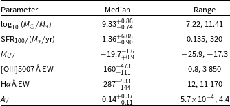
Physical parameter median, 1
 $\sigma$
and sample range for our final sample of 230 galaxies.

Table 2. Long description
A table with three columns and six rows, detailing the median and range of various physical parameters for a sample of 230 galaxies. The columns are labeled ‘Parameter’, ‘Median’, and ‘Range’. The parameters listed are log10(M/M sun symbol), SFR100(M sun symbol/yr), MUV, [OIII]5007Å EW, Hα EW, and AV. Each row provides the median value and range for each parameter. For example, the first row shows log10(M/M sun symbol) with a median of 9.33 and a range from 7.22 to 11.41.
2.8. Sample introduction
Refer to Table 2 for the median physical properties and parameter ranges of the sample. Using the main-sequence relation defined by Speagle et al. (Reference Speagle, Steinhardt, Capak and Silverman2014) (their Equation 28), we find that only
 $\sim$
15% of galaxies lie within the expected main-sequence limits (Figure 4). Defining recent burst activity as
 $\mathrm{SFR_{10}/SFR_{100} \gt 9}$
, such that the recent star formation rate exceeds the estimated 100 Myr average by a factor of nine, yields
 $\sim$
24% of the sample. Conversely, defining declining or quiescent star formation as
 $\mathrm{SFR_{10}/SFR_{100} \lt 1}$
yields
 $\sim$
20% of galaxies.
Stellar Mass vs Star Formation rate (averaged over 100 Myr) for our OutThere sample of 230 galaxies. Orange diamonds correspond to equal-population bin medians, and their error-bars reflect the 16–84th percentile ranges. The main sequence relation for
 $z=2$
from Speagle et al. (Reference Speagle, Steinhardt, Capak and Silverman2014) is indicated in black with upper and lower limits indicated in grey. Blue diamonds reflect galaxies where
 $\mathrm{\frac{H\alpha^{Model}-H\alpha}{H\alpha}\gt +2}$
. Our sample lies largely below the Main Sequence.

 $\mathrm{[OIII]5007}$
Å EW vs
 $\mathrm{H\alpha}$
Å EW for our OutThere sample of 230 galaxies. Orange diamonds correspond to equal-population bin medians (excluding limits), and their error-bars reflect the 16–84th percentile ranges. Blue diamonds reflect galaxies where
 $\mathrm{\frac{H\alpha^{Model}-H\alpha}{H\alpha}\gt +2}$
. Our sample spans a notable range in both EWs, with
 $\sim$
23% within the extreme emission line definition of Jaiswar et al. (Reference Jaiswar, Gupta, da Cunha, Trott, Harshan, Battisti and Forrest2024).

(a) (Left) UV slope vs
 $\mathrm{\xi_{ion}^{HII}}$
(Right) M
 $_{UV}$
vs
 $\mathrm{\xi_{ion}^{HII}}$
(b) (Left) Stellar mass M
 $_*$
vs
 $\mathrm{\xi_{ion}^{HII}}$
(Right) sSFR vs
 $\mathrm{\xi_{ion}^{HII}}$
. Opacity of data-points inversely proportional to BEAGLE SED reduced
 $\chi^2$
so that better fits are more opaque. Orange diamonds correspond to equal-population bin medians, and their error-bars reflect the 16–84th percentile ranges. Points from Harshan et al. (Reference Harshan2024) plotted as green stars. We find no significant Spearman correlations between
 $\mathrm{\xi_{ion}^{HII}}$
and any of these parameters.

The range of
 ${M_{UV}}$
values indicates that the sample is generally brighter than those typically studied in the high-redshift literature. Additionally, a significant fraction of the sample (
 $\sim$
23%) would be classified as extreme [OIII]
 $\lambda5007$
equivalent width emitters, with
 $\mathrm{EW([OIII]\lambda5007) \gt 400,\mathring{A}}$
(Figure 5; Jaiswar et al. Reference Jaiswar, Gupta, da Cunha, Trott, Harshan, Battisti and Forrest2024). The extreme [OIII]
 $\lambda5007$
and H
 $\alpha$
equivalent widths present in the sample allow us to probe the applicability of the
 $\mathrm{\xi_{ion}}$
relations derived by Tang et al. (Reference Tang, Stark, Chevallard and Charlot2019) and Boyett et al. (Reference Boyett2024) in regimes of extreme line emission.
3. Results
3.1.
$\mathrm{\xi_{ion}}$

The ionising photon production efficiency is important to constrain for the purpose of understanding the ionising photon budget in the EoR. Deriving correlations to other physical parameters that are easier to constrain for large samples is vital to draw broader conclusions on the evolutionary history of the Universe in this epoch. Here we explore the relationship of
 $\mathrm{\xi_{ion}^{HII}}$
to physical parameters determined from BEAGLE.
3.1.1. UV parameters
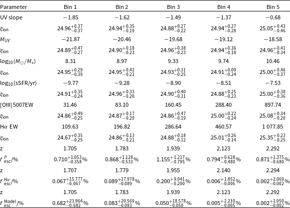
The UV slope is calculated as the slope of UV luminosity between 1 500 and 2 500Å in the modelled SED from BEAGLE. (Figure 6). We report the median
 $\mathrm{\xi_{ion}^{HII}}$
of each UV slope bin from bluest to reddest in Table 3. The assumed dependence of
 $\mathrm{\xi_{ion}}$
on the massive stellar population and the expected correlation of a young stellar population to a bluer UV slope suggest that this relationship should too, be negatively correlated. Bluer galaxies should be more efficient ionising photon producers. However, for our sample, we do not find a significant Spearman correlation (
 $p\gt 0.05$
). We note, however, that when excluding data-points within the reddest bin, we do find a significant positive correlation (
 $\rho =0.28$
,
 $p\lt 7.1\times10^{-4}$
). Harshan et al. (Reference Harshan2024) and Lam et al. (Reference Lam2019) similarly find no correlation, also using a smaller dynamical range of UV slopes, while Castellano et al. (Reference Castellano2023) and Bouwens et al. (Reference Bouwens, Smit, Labbé, Franx, Caruana, Oesch, Stefanon and Rasappu2016) find a negative correlation over a wider range. The difficulty with associating the UV slope with stellar age comes with its degeneracy with dust attenuation. In our sample, the reddest galaxies also have the largest A
 $_V$
(see Figure 3).
 $\xi_{\mathrm{ion}}$
(erg
 $^{-1}$
Hz) and
 $f{_{\rm esc}}$
(%) measured in five bins. For each parameter, bin centres are shown in the first row, followed by either
 $\xi_{\mathrm{ion}}$
or
 ${f_{\rm esc}}$
. Bins are equal-population bin medians with the 16–84th percentile ranges reported.

Table 3. Long description
A table comparing various parameters across five bins. The table has 15 rows and 6 columns, including headers. The columns are labeled as Bin 1, Bin 2, Bin 3, Bin 4, and Bin 5. The rows are labeled with different parameters: UV slope, MUV, SION, log10(M/M⊙), log10(sSFR/yr), [OIII]5007EW, Hα EW, z, fesc/% z, fesc/% z, and fModel/%. Each row provides values for each bin. For example, the first row under UV slope shows values like -1.85 for Bin 1 and -0.68 for Bin 5. The table captures the median values and their respective 1684th percentile ranges for each parameter across the five bins.
We calculate the median of each
 $M{_{UV}}$
bin in Table 3. We report no significant Spearman correlation (
 $p\gt 0.05$
) though this hinges on the inclusion of the brightest bin (
 $\rho =0.19$
,
 $p\lt 0.02$
without it). Harshan et al. (Reference Harshan2024) finds a steep positive correlation at
 $z\gt 5$
and suggests that fainter galaxies are more efficient producers of ionising emission, though for our sample at
 $z\sim 1.5$
this does not appear to be the case. In both the case of the
 $\beta$
and
 ${M_{UV}}$
correlations, removing data-points within the reddest/brightest bin improves the significance of the correlation significantly.
3.1.2. Stellar parameters
The stellar mass (log
 $_{10}(M_*/M_\odot$
)) and specific star formation rate (log
 $_{10}$
(sSFR/yr
 $^{-1}$
)) are each derived from the BEAGLE best fit SED (Figure 6). We derive bin-median stellar masses from the least to most massive in Table 3. We do not find a significant Spearman correlation with this parameter (
 $p\gt 0.05$
), suggesting that more massive galaxies do not produce less ionising emission per non-ionising UV emission. This is unexpected as the
 $\mathrm{\xi_{ion}}$
dependence on a young stellar population would be linked to its mass via the age-mass relation. We note, however, that this correlation is improved when removing data-points within the most massive bin with sample variance roughly 1.6
 $\times$
that of the other bins. Harshan et al. (Reference Harshan2024), Lam et al. (Reference Lam2019), Castellano et al. (Reference Castellano2023) find negative slopes with a similarly large intrinsic scatter, albeit with a stronger overall ionising efficiency for a less massive, higher redshift sample.
We compute the sSFR bin-medians in Table 3 from most negative to most positive. We do not find a significant Spearman correlation in these parameters. Similar works by Harshan et al. (Reference Harshan2024) also using the SED derived SFR, finds only a weak positive correlation at
 $z\gt 5$
despite a strong theoretical support to this relationship. Proportionally high star formation rates indicate young stellar populations that should have a large contribution to the ionising photon production. Castellano et al. (Reference Castellano2023) finds this correlation to be strong in their 2
 $\lt z\lt$
5 sample, however, both of these works claim increasing scatter and weaker correlation toward the lower sSFR end where the majority of our sample lies (sSFR
 $\lt -8$
). This correlation may therefore hold better for starburst galaxies at higher redshifts than our sample.
3.1.3 Correlations to equivalent widths
The [OIII]5007 and H
 $\alpha$
EW are derived from the OutThere NIRISS spectra (Figure 7). We report the bin medians from lowest to highest [OIII]5007 Å EW in Table 3 and find a significant Spearman correlation (slope = 0.16, intercept = 24.62, Spearman rank = 0.26
 $p\lt 5.0\times 10^{-5}$
). The [OIII]5007 emission line is associated with star forming regions, and theoretically this suggests large [OIII]5007 EW should correlate with young stellar populations which our results corroborate. We highlight the extreme [OIII]5007 region and find these sources exhibiting the largest
 $\mathrm{\xi_{ion}^{HII}}$
. Tang et al. (Reference Tang, Stark, Chevallard and Charlot2019) and Boyett et al. (Reference Boyett2024) find a strict correlation between
 $\mathrm{\xi_{ion}^{HII}}$
measurements and the dust-corrected, BEAGLE SED
 $L_{UV}$
which contains both stellar and nebular contributions. These appear to be dependent on the sample redshift (Tang et al. Reference Tang, Stark, Chevallard and Charlot2019; Boyett et al. Reference Boyett2024). We find that the correlations hold within 3
 $\sigma$
for our sample spanning a wider redshift range and constraining the lower dynamical range of [OIII]5007 EW
 $\lt 225$
. Tang et al. (Reference Tang, Stark, Chevallard and Charlot2019) predicted deviations below [OIII]5007 EW
 $\lt$
225, and we do find a larger scatter below this limit (see Table 3), which reduces the measured slope and Spearman rank of our sample by comparison to a relation drawn only considering values above this (slope = 0.413, intercept = 23.94, Spearman rank = 0.352,
 $p\lt 6.3\times 10^{-4}$
).
(Left) [OIII]5007 EW vs
 $\mathrm{\xi_{ion}^{HII}}$
and (Right) H
 $\alpha$
EW vs
 $\mathrm{\xi_{ion}^{HII}}$
. Opacity of data-points inversely proportional to BEAGLE SED reduced
 $\chi^2$
so that better fits are more opaque. Orange diamonds correspond to equal-population bin medians, and their error-bars reflect the 16–84th percentile ranges. Region above EW=750 Å indicated by the green shaded region as in Boyett et al. (Reference Boyett2024), and points derived from Boyett et al. (Reference Boyett2024) in pink and cyan stars. Trends from Tang et al. (Reference Tang, Stark, Chevallard and Charlot2019), Boyett et al. (Reference Boyett2024) indicated by black, pink and cyan lines. We find significant Spearman correlations between
 $\mathrm{\xi_{ion}^{HII}}$
and each of [OIII]5007 EW (
 $\rho$
= 0.26) and H
 $\alpha$
EW (
 $\rho$
= 0.65) in our samples.

The H
 $\alpha$
EW is itself correlated with the H
 $\alpha$
flux used to derive
 $\mathrm{\xi_{ion}^{HII}}$
as a tracer of LyC emission. We calculate the bin averages of this relation in Table 3 from lowest to highest EW. We also report a clear positive monotonic relationship (slope = 0.53, intercept = 23.65, Spearman rank = 0.65,
 $p\lt 6.4\times 10^{-29}$
) that matches that found in Tang et al. (Reference Tang, Stark, Chevallard and Charlot2019) within 1
 $\sigma$
. Harshan et al. (Reference Harshan2024) finds a similar slope (0.7) and Spearman coefficient (0.6) at
 $z\gt 5$
.
3.2.
${\boldsymbol{f}_{\rm esc}}$

The escape fraction of ionising radiation is necessary to constrain alongside the ionising photon production efficiency to determine the ionising budget per galaxy. The challenge with estimating this value beyond the Local Universe is the direct detection of LyC which is readily absorbed by the IGM even at intermediate redshifts (Inoue et al. Reference Inoue, Shimizu, Iwata and Tanaka2014). Here we explore the correlations of our escape fraction estimates to physical parameters determined from BEAGLE to test our methodology and recover potential correlations. Of the 233 galaxies in our sample, 199 have measurable
 $f{_{\rm esc}}$
values after excluding systems with physically inconsistent spectral and SED-derived properties. Specifically, we remove galaxies where the total ionising photon budget,
 $N\mathrm{_{ion}}$
, inferred from the SED model is lower than that implied by the dust-corrected H
 $\alpha$
luminosity, as well as cases yielding non-physical escape fractions (
 $\,f\mathrm{_{\!esc}}\lt 0$
or
 $f\mathrm{_{\!esc}}\gt 1$
).
Escape fraction of Lyman Continuum radiation calculated using (Top) the UV slope, and the theoretical approach described in Section 2.6 using spectral H
 $\alpha$
(Middle) and using modelled H
 $\alpha$
(Bottom). Region above 1% escape fraction indicated by the green shaded region. Opacity of data-points inversely proportional to BEAGLE SED reduced
 $\chi^2$
so that better fits are more opaque. Orange diamonds correspond to equal-population bin medians, and their error-bars reflect the 16–84th percentile ranges. Cullen et al. (Reference Cullen2024) sample averages for
 $z\lt 10.5$
and
 $z\gt 10.5$
shown in the UV slope panel using the same method. Papovich et al. (Reference Papovich2026) uses the SED modelled
 ${f_{\rm esc}}$
which we include in the bottom panel for comparison. Our sample at
 $z\sim 2$
has a much lower
 ${f_{\rm esc}^\beta}$
and a much more scattered
 ${f_{\rm esc}^{\rm Model}}$
than the comparison samples.

The majority of the following analysis is performed using the method described in Section 2.6, which derives the escape fraction we refer to as
 $f_{\rm esc}^{{\rm H}\alpha}$
. We denote the UV slope derived
 ${f_{\rm esc}}$
as
 $f_{\rm esc}^\beta$
and distinguish
 ${f_{\rm esc}}$
calculated from the spectral H
 $\alpha$
from the SED model H
 $\alpha$
as
 $f_{\rm esc}^{{\rm H}\alpha}$
and
 $f_{\rm esc}^{\rm Model}$
, respectively.
Our methodology is not directly comparable to much of the existing literature in this field. We do not treat the
 ${f_{\rm esc}}$
as a free parameter in the SED model fit. The closest comparisons are studies that derive
 ${f_{\rm esc}}$
directly from SED models, where the escape fraction is incorporated into the fitting procedure (Giovinazzo et al. Reference Giovinazzo2026; Papovich et al. Reference Papovich2026). We instead use the SED model to inform the total theoretical ionising budget and the spectroscopic H
 $\alpha$
(dust corrected using the SED model) as our probe of its absorption by the nebula. Combined with the dust absorption estimation (using the SED model), this results in a large dynamical range of possible
 $f_{\rm esc}^{{\rm H}\alpha}$
compared to methods relying on selected priors. We therefore treat extremely low values of
 $f_{\rm esc}^{{\rm H}\alpha}$
as lower limits, and report correlations both including and excluding these systems.
Studies deriving SED-modelled
 ${f_{\rm esc}}$
typically impose lower priors of 0.1–0.01%. However, the physical plausibility of smaller escape fractions is not constrained by the practical limits adopted in SED fitting. We therefore adopt 0.01% as our fiducial lower limit, and vary this between 0.1% and no limit to verify that the qualitative behaviour of the correlations remains unchanged when varying the floor.
3.2.1 Redshift evolution
Here we report the redshift evolution of the
 ${f_{\rm esc}}$
for this
 $z\sim 2$
sample for each of the three derivation methods (Figure 8).
We report no
 $f^\beta_{\rm esc}$
evolution across redshift (
 $p\gt 0.05$
). We find that our sample at
 $z\sim 2$
is consistently below the escape fraction found in high redshift samples using the same technique (Cullen et al. Reference Cullen2024) (
 $\,{f_{\rm esc}^\beta}$
= 5% and
 ${f_{\rm esc}^\beta}$
= 19% for the
 $z\lt 10.5$
and
 $z\gt 10.5$
ranges, respectively). The
 ${f_{\rm esc}^\beta}$
derivation is proportional to the UV slope, and hence our redder sample lies below the much bluer, early-universe counterparts. Theoretically, the
 ${f_{\rm esc}^\beta}$
is shown to increase with increasing redshift (Chisholm et al. Reference Chisholm2022) as it is inversely proportional to the UV slope which generally decreases with increasing redshift. As our sample spans a short redshift range it is likely that our dynamical range hinders the estimation of a significant correlation.
We find that our theoretical escape fraction methods overlap with traditional SED fit
 ${f_{\rm esc}}$
(Papovich et al. Reference Papovich2026) at high redshifts albeit with more scatter. This method is similar to our
 $f_{\rm esc}^{\rm Model}$
method in that all inputs are taken from the SED model, though our implementation instead uses a simplified escape-path framework rather than incorporating the escape fraction directly as a goodness-of-fit parameter within the SED fitting procedure. The large scatter observed in the theoretical escape fractions is likely a product of the many competing variables in this approach, relying on both modelled dust corrections, dust escape fractions and theoretical ionising photon production from the photo-ionisation model, as well as the spectroscopic H
 $\alpha$
, each of which can vary substantially per galaxy. The bin median values, however, are within the theoretical ranges reported by Matthee et al. (Reference Matthee, Sobral, Best, Khostovan, Oteo, Bouwens and Röttgering2017), Grazian et al. (Reference Grazian2017) and determined for galaxies in a similar
 ${M_{UV}}$
range by Finkelstein et al. (Reference Finkelstein2019). Grazian et al. (Reference Grazian2017) finds that at a slightly higher redshift of
 $3.27\lt z\lt 3.4$
galaxies brighter than
 $M_{1\,500}\sim-19$
exhibit an upper limit of
 $f_{\rm esc} \lt 1.7\%$
. Studying H
 $\alpha$
and Ly
 $\alpha$
emitters at
 $z\sim 2.2$
, Matthee et al. (Reference Matthee, Sobral, Best, Khostovan, Oteo, Bouwens and Röttgering2017) finds
 $f_{\rm esc} \lt 6.4\%$
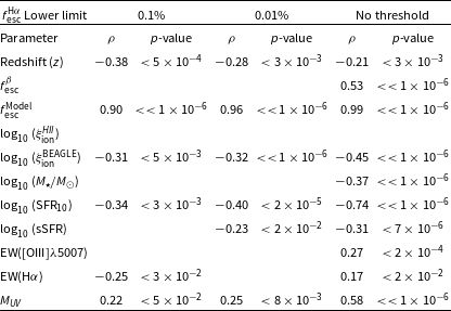
by directly studying the LyC using GALEX/NUV and mean-stacking. We find that our theoretical methods have significant negative correlations to the redshift at each threshold (see Table 4 for correlations to
 $f_{\rm esc}^{{\rm H}\alpha}$
) (
 $\rho = -0.35, p\lt 2\times10^{-3}$
at 0.1%,
 $\rho = -0.27$
,
 $p\lt 4\times10^{-3}$
at 0.01% and
 $\rho = -0.21$
,
 $p\lt 3\times10^{-3}$
with no lower limit for
 $f_{\rm esc}^{\rm Model}$
).
This negative trend aligns with observations above
 $z\gt 4.5$
made by Papovich et al. (Reference Papovich2026) using SED modelling, suggesting that early universe galaxies contained much of their ionising photon production. As discussed, low redshift studies correlating the UV slope derived
 ${f_{\rm esc}^\beta}$
with redshift imply an increasing escape fraction with redshift (Chisholm et al. Reference Chisholm2022; Flury et al. Reference Flury2022) and even with the simulation based escape fraction from Finkelstein et al. (Reference Finkelstein2019) and with the results of the THESAN simulations (Yeh et al. Reference Yeh2023).
These contrary results should be considered in terms of the distinctions in their method of derivation. The THESAN simulations incorporate radiative transfer modelling that self-consistently calculates the ionisation state of hydrogen gas from the radiation field (Kannan et al. Reference Kannan, Garaldi, Smith, Pakmor, Springel, Vogelsberger and Hernquist2022). Studies such as Papovich et al. (Reference Papovich2026) use the photo-ionisation modelling incorporated within the SED model to self-consistently determine the production and escape of ionising photons given the synthesised stellar population. Our approach first confirms the agreement of the spectroscopically observed nebular emission with the modelled spectrum and uses this to confirm the viability of the SED modelled stellar population before using the total modelled ionising budget to self-consistently determine the ionising escape using our two-layer escape model. By contrast, the Finkelstein et al. (Reference Finkelstein2019) model is calibrated empirically using data from Finkelstein (Reference Finkelstein2016) at
 $z\gt 4$
, as is the Chisholm et al. (Reference Chisholm2022) model using empirical, low redshift LyC observations.
(Left)
 ${f_{\rm esc}}$
determined from the Chisholm et al. (Reference Chisholm2022) relation (
 ${f_{\rm esc}^\beta}$
) vs determined from our spectroscopic derivation (
 ${f_{\rm esc}^{{\rm H}\alpha}}$
). (Right)
 $\mathrm{\xi_{ion}^{HII}}$
vs the
 ${f_{\rm esc}^{{\rm H}\alpha}}$
. Lower limits indicate
 ${f_{\rm esc}^{{\rm H}\alpha}}$
values below the 30th percentile (
 $\lt$
 $1.5\times10^{-6}$
). Orange diamonds correspond to equal-population bin medians (excluding limits), and their error bars reflect the 16–84th percentile ranges. Green shaded region indicates
 ${f_{\rm esc}^{{\rm H}\alpha}\gt 1\%}$
(64/199 sources) while black and red dotted lines represent
 ${f_{\rm esc}^{{\rm H}\alpha} = 0.1\%}$
and
 ${f_{\rm esc}^{{\rm H}\alpha} = 0.01\%}$
respectively. We do not find a significant correlation with either parameter.

Spearman correlation coefficients (
 $\rho$
) and associated p-values between
 ${{f_{\rm esc}^{{\rm H}\alpha}}}$
and galaxy properties for different lower escape fraction thresholds. cells reflecting correlations with p-value
 $\gt$
0.05 are highlighted in green, while cells highlighted in red fall above this.

Table 4. Long description
A table with four rows and three columns comparing Spearman correlation coefficients and p-values between escape fraction and galaxy properties at different thresholds. The columns are labeled with different lower limit thresholds: 0.1 percent, 0.01 percent, and No threshold. The rows are labeled with different parameters: Redshift (z), f esc, log 10 (s SFR), EW[OIII]+5007, EW(H alpha), and M UV. Each cell contains the correlation coefficient and p-value for the respective parameter and threshold. Notable trends include significant negative correlations to redshift at each threshold, with varying p-values indicating the strength of these correlations.
3.2.2. Ionising parameters
We do not find significant correlations between
 $f_{\rm esc}^{{\rm H}\alpha}$
and
 $f^\beta_{\rm esc}$
when excluding the lower limit values, though find a fairly strong correlation when including the full sample (see Table 4 and Figure 9). Theoretically as these quantities are intended as descriptions of one phenomenon, their correlation is logical. As discussed in Section 3.2.1, however, this is not the case as the derivation methods are incomparable. By contrast, the theoretically equivalent
 $f_{\rm esc}^{\rm Model}$
approach correlates very strongly.
We find no significant correlations to the
 $\mathrm{\xi_{ion}^{HII}}$
despite both parameters relying on the same dust corrected H
 $\alpha$
flux. Considering that the ionising photon production efficiency is a reflection of the intrinsic ionising photon budget, and that our escape fraction model uses the SED model ionising photon budget, this leaves only the dust component of the escape fraction calculation as a distinguishing input. Intriguingly, the internal SED model
 $\mathrm{\xi_{ion}}$
does significantly correlate with
 $f_{\rm esc}^{{\rm H}\alpha}$
, suggesting that as the escape fraction rises the production efficiency drops. Theoretically speaking, ionising photons are largely produced from young massive stars which spend significant portions of their lives within the birth clouds from which they formed. Escaping photons primarily originate in these systems once escape paths are cleared by feedback mechanisms and by previous ionisation. Standard population models see the production efficiencies of these systems decline rapidly with the ageing population which agrees with our findings (Ma et al. Reference Ma, Kasen, Hopkins, Faucher-Giguère, Quataert, Kereš and Murray2015).
 ${M_{UV}}$
vs
 ${f_{\rm esc}}$
determined from our spectroscopic derivation (
 $\,{f_{\rm esc}^{{\rm H}\alpha}}$
). Lower limits indicate
 ${f_{\rm esc}^{{\rm H}\alpha}}$
values below the 30th percentile (
 $\lt$
 $1.5\times10^{-6}$
). Orange diamonds correspond to equal-population bin medians (excluding limits), and their error-bars reflect the 16–84th percentile ranges. Green shaded region indicates
 ${f_{\rm esc}^{{\rm H}\alpha}\gt 1\%}$
(64/199 sources) while black and red dotted lines represent
 ${f_{\rm esc}^{{\rm H}\alpha} = 0.1\%}$
and
 ${f_{\rm esc}^{{\rm H}\alpha} = 0.01\%,}$
, respectively. Blue vertical line indicates the
 ${M_{UV} = -19}$
cutoff. We compare our results to LyC selected studies (Steidel et al. 2018; Wang et al. Reference Wang2025) as well as non-selected stacks (Cowie et al. Reference Cowie, Barger and Trouille2009; Siana et al. Reference Siana2010) and the Finkelstein et al. (Reference Finkelstein2019) simulation at
 $z=4-6$
. We find significant positive correlations between the
 ${f_{\rm esc}^{{\rm H}\alpha}}$
and
 ${M_{UV}}$
parameters (
 $\rho \gt 0.22$
) suggesting that fainter
 ${M_{UV}}$
galaxies have larger escape fractions.

3.2.3.
${M_{UV}}$

We report significant positive correlations between
 $f_{\rm esc}^{{\rm H}\alpha}$
and
 ${M_{UV}}$
at each threshold (Figure 10). This is in contrast to the findings from Papovich et al. (Reference Papovich2026) and Giovinazzo et al. (Reference Giovinazzo2026), neither of which found correlations in this comparison. Studies such as Grazian et al. (Reference Grazian2017) point to fainter sources having larger escape fractions, though with caveats for observational depth, which would agree with our findings. The spectroscopic selection introduces a bias to brighter sources, so it is entirely plausible that this correlation is a product of selection bias. To mitigate potential faint-end selection biases, we further report significant correlations at each threshold with a faint-end limit of
 ${M_{UV}\lt -19}$
(
 $\rho = 0.34, p\lt 2\times10^{-2}$
for 0.1%,
 $\rho$
= 0.32,
 $p\lt 8\times10^{-3}$
for 0.01% and
 $\rho$
= 0.61,
 $p\lt\lt 1\times10^{-6}$
with no threshold). Our results appear to support the faint-galaxy EoR contribution narrative (Kulkarni et al. Reference Kulkarni, Keating, Haehnelt, Bosman, Puchwein, Chardin and Aubert2019), as we find increasing
 $f_{\rm esc}^{{\rm H}\alpha}$
with fainter sources.
We also contrast our sample to multiple direct observations at varying redshift (Cowie et al. Reference Cowie, Barger and Trouille2009; Siana et al. Reference Siana2010; Steidel et al. Reference Steidel and Bogosavljević2018; Wang et al. Reference Wang2025) and to simulated estimations (Finkelstein et al. Reference Finkelstein2019) at high redshift as a benchmark for our findings. These direct studies tend to use the ratio of detected photons at 880–912 Å normalised by the flux found at the non-ionising UV 1 500 Å mark to calculate the escape fraction (Steidel et al. Reference Steidel, Pettini and Adelberger2001), making their methodology fundamentally different from the H
 $\alpha$
-based approach adopted here.
We find a range of observed escape fractions in these samples. Steidel et al. (Reference Steidel and Bogosavljević2018) prioritised star-forming Lyman Break Galaxies and AGN at
 $z\sim3$
, reporting a
 $12\pm 0.1$
% escape fraction across the whole sample using their Intergalactic + Circumgalactic Medium (IGM+CGM) absorption calculation. Wang et al. (Reference Wang2025) stacks two sets of 28 galaxies with average redshifts of
 $\sim$
2.4 and
 $\sim$
2.7, finding no significant (
 $2\sigma$
) detection of LyC flux in either stack, and setting
 $1\sigma$
upper limits of 5% and 26%, respectively. These observations indicate much larger escape fractions than is determined in most of our sample, possibly due to the sample selection and survey design of ground based observation as noted in Finkelstein et al. (Reference Finkelstein2019). At lower redshift, Siana et al. (Reference Siana2010) found a stacked upper limit of 2% while Cowie et al. (Reference Cowie, Barger and Trouille2009) found no significant detection when estimating the relative escape fraction. The relative escape fraction differs from the absolute escape fraction by not including the dust correction factor, so these upper limits represent a generous depiction of LyC escape. Our sample median of 2% escape fraction agrees more closely with the findings of Siana et al. (Reference Siana2010) and Cowie et al. (Reference Cowie, Barger and Trouille2009), as well as with the assumed trajectory of the Finkelstein et al. (Reference Finkelstein2019) simulation, found to approach 0.01% at
 $z\sim4$
. Together, these comparisons suggest that characteristic, population-averaged escape fractions inferred from non-LyC tracers, as well as from non-targeted LyC studies, are typically much lower than those measured in observations designed to identify the strongest LyC-leaking galaxies.
3.2.4. Stellar parameters
We do not find a significant correlation between the
 $f_{\rm esc}^{{\rm H}\alpha}$
and stellar mass besides when considering the full sample (see Table 4 and Figure 11). Theoretically, low stellar masses correlate with high escape fractions due to the shallow gravitational potential wells produced by the halo (Finkelstein et al. Reference Finkelstein2019). However, Yeh et al. (Reference Yeh2023) finds no such clear trend, reporting a largely ambivalent relationship between stellar mass and ionising photon escape. We note that the median stellar mass of the galaxies below the 0.01% threshold (
 ${\log_{10}(M_*/M_\odot = 9.64^{+1.09}_{-1.16})}$
) is higher than those above it (
 ${\log_{10}(M_*/M_\odot = 9.08^{+0.71}_{-0.48})}$
) which extends the contributing mass range and potentially leads to the theoretically expected negative correlation.
(a) (Left) Stellar mass vs
 ${f_{\rm esc}^{{\rm H}\alpha}}$
and (Right) Mass normalised star formation rate (sSFR) vs
 ${f_{\rm esc}^{{\rm H}\alpha}}$
. (b) (Left) Short timescale averaged SFR (10 Myr) and (Right) 100 Myr timescale averaged SFR vs
 ${f_{\rm esc}^{{\rm H}\alpha}}$
. Lower limits indicate
 ${f_{\rm esc}^{{\rm H}\alpha}}$
values below the 30th percentile (
 $\lt$
 $1.5\times10^{-6}$
). Orange diamonds correspond to equal-population bin medians (excluding limits), and their error-bars reflect the 16–84th percentile ranges. Green shaded region indicates
 ${f_{\rm esc}^{{\rm H}\alpha}\gt 1\%}$
(64/199 sources) while black and red dotted lines represent
 ${f_{\rm esc}^{{\rm H}\alpha} = 0.1\%}$
and
 ${f_{\rm esc}^{{\rm H}\alpha} = 0.01\%}$
, respectively. We observe a negative correlation in the sSFR suggesting that galaxies with relatively high rates of star formation do not allow LyC escape. We observe negative correlations to only the short timescale SFR, indicating that more bursty star forming galaxies do not have large escape fractions.

We find significant negative correlations of
 $f_{\rm esc}^{{\rm H}\alpha}$
to the star formation rate averaged over the last 10Myr (
 $\mathrm{log_{10}(SFR_{10}/(M_\odot/yr))}$
, with increasing magnitude with the inclusion of the full sample. We also find that changing the averaging to 100 Myr significantly diminishes this trend, only becoming significant without thresholds (
 $\rho = -0.56$
,
 $p\lt\lt 1\times10^{-6}$
). We report a slight negative correlation of
 $f_{\rm esc}^{{\rm H}\alpha}$
to the specific SFR (sSFR/yr) at a threshold of 0.01%
 $f_{\rm esc}^{{\rm H}\alpha}$
. The short timescale SFR is used in BEAGLE to determine the population of massive stars which contribute significantly to the ionising budget. These stars also significantly contribute to the H
 $\alpha$
emission, which in our model is interpreted as higher rates of LyC absorption. As discussed in Papovich et al. (Reference Papovich2026), galaxies with large ionising budgets at
 $z\gt 4.5$
are found to have low escape fractions. Comparing to simulations at the EoR (Yeh et al. Reference Yeh2023) and observational constraints based on high redshift LyC leakers (Naidu et al. Reference Naidu, Tacchella, Mason, Bose, Oesch and Conroy2020), galaxies with a high SFR (100 Myr average) tend to have larger
 ${f_{\rm esc}}$
, where we find no correlation within the same
 ${f_{\rm esc}}$
threshold for this SFR timescale. Our results do corroborate those from Giovinazzo et al. (Reference Giovinazzo2026) which report no significant correlation to the SFR density.
3.2.5. Emission line EW
We do not find significant correlations between
 $f_{\rm esc}^{{\rm H}\alpha}$
and the [OIII]5007 EW using either threshold, but do find a slight positive correlation with the full sample (see Table 4 and Figure 12). The [OIII]5007 EW is not traditionally used as a proxy for
 ${f_{\rm esc}}$
, favouring instead the O
 $\mathrm{_{32}}$
ratio as a more geometrically considerate method (Jaskot & Oey Reference Jaskot and Oey2013). It is, however, used in selecting extreme emission line galaxies (Jaiswar et al. Reference Jaiswar, Gupta, da Cunha, Trott, Harshan, Battisti and Forrest2024) which may imply LyC leaker behaviour. Saxena et al. (Reference Saxena2022) for example, finds that in their LyC leaker sample at
 $3.11 \lt z \lt 3.53$
, the
 ${f_{\rm esc}}$
has a slight positive correlation with the combined [OIII]5007+H
 $\beta$
EW. The blended emission line and sample selection however limit the utility of this direct comparison.
(Left)
 $\mathrm{[OIII]}\,5007\,\lambda\mathring{\textrm{A}}$
EW and (Right)
 $\mathrm{H\alpha}\,\mathring{\textrm{A}}\,$
EW vs
 ${f_{\rm esc}^{H\alpha}}$
. Lower limits indicate
 ${f_{\rm esc}^{{\rm H}\alpha}}$
values below the 30th percentile (
 $\lt 1.5\times10^{-6}$
). Orange diamonds correspond to equal-population bin medians (excluding limits), and their error-bars reflect the 16–84th percentile ranges. Green shaded region indicates
 ${f_{\rm esc}^{{\rm H}\alpha}\gt 1\%}$
(64/199 sources) while black and red dotted lines represent
 ${f_{\rm esc}^{{\rm H}\alpha} = 0.1\%}$
and
 ${f_{\rm esc}^{{\rm H}\alpha} = 0.01\%}$
, respectively. We do not observe significant correlations to the
 $\mathrm{[OIII]}\,5007\,\lambda\mathring{\textrm{A}}$
, while the
 $\mathrm{H\alpha}\,\mathring{\textrm{A}}\,$
EW appears to be negatively correlated with the ionising escape. This may be an underlying degeneracy with bursty star formation.

We find a significant negative correlation between
 $f_{\rm esc}^{{\rm H}\alpha}$
and the H
 $\alpha$
EW for
 $f{_{\rm esc}}\gt 0.1\%$
which flips without a threshold, implying distinct behaviour in the high
 $f_{\rm esc}^{{\rm H}\alpha}$
regime. In the low
 $f_{\rm esc}^{{\rm H}\alpha}$
regime, dust becomes a dominating component of this calculation while in the high
 $f_{\rm esc}^{{\rm H}\alpha}$
regime the H
 $\alpha$
EW is likely suppressed by photon leakage. The distinct behaviours are therefore likely to be consequences of the
 $f_{\rm esc}^{{\rm H}\alpha}$
model’s sensitivity to different dominant sources of attenuation across regimes, transitioning from dust-dominated corrections at low escape fractions to geometry- and density-bounded effects that directly reduce nebular line emission at higher escape fractions.
4. Summary and conclusions
We report a new sample of 230 galaxies between
 $1.3\lt z\lt 2.6$
with robust H
 $\alpha$
fluxes from the HUDF-N pointings of the pure-parallel JWST/NIRISS program; OutThere in terms of their ionising photon production and escape. We use this sample to test correlations between physical parameters, nebular emission lines and ionising emission properties drawn at higher redshifts with smaller dynamical ranges.
-
1. We find no significant correlation of
$\mathrm{\xi_{ion}^{HII}}$
to the UV slope or sSFR, possibly due to the redder and less star forming galaxies of this sample when contrasted with the high redshift studies. We also do not find that the UV magnitude has any notable correlation with
$\mathrm{\xi_{ion}^{HII}}$
as found in high redshift samples, indicating that efficient LyC producers being prevalent in fainter sources may not be true of the general population at
$z\sim 2$
. -
2. We do not find the expected anti-correlation of
$\mathrm{\xi_{ion}^{HII}}$
to stellar mass. The sample is particularly scattered at the high mass end which may prevents a significant correlation being defined. -
3. We corroborate the findings of nebular emission line comparisons to
$\mathrm{\xi_{ion}^{HII}}$
both at the same and higher redshifts and extend the dynamical range of equivalent widths to the lowest range. We find both in the case of [OIII]5007 and H
$\alpha$
that an increasing EW correlates with an increasing
$\mathrm{\xi_{ion}^{HII}}$
. -
4. We find no correlations between the UV slope derived escape fraction and redshift and find similar values to those reported at
$z\sim 2$
when using the Chisholm et al. (Reference Chisholm2022) UV slope correlation. We find that our theoretical
${f_{\rm esc}}$
’s are more varied, finding both much larger and much smaller escape fractions than those found by the empirical relation though still within theoretical limits. We do find tentative correlations to redshift in these methods, however, these methods are purely theoretical and require further testing. -
5. We find consistent positive correlations between the H
$\alpha$
${f_{\rm esc}}$
and
$M{_{UV}}$
, indicating that fainter galaxies may have more notable LyC escape fractions. -
6. We find that our escape fractions do not correlate with stellar mass or [OIII]5007 Å EW above the 0.01% escape threshold. Intuitively the lower mass and high stellar activity indicators suggest shallow gravitational wells and hard ionising emissions potentially forming escape routes. However, our
${f_{\rm esc}}$
limits remove the highest mass and lowest [OIII]5007 emitters which contribute to the correlation. -
7. The H
$\alpha$
${f_{\rm esc}}$
correlation is threshold dependent, with the direction reversing for the lowest
${f_{\rm esc}}$
galaxies, indicating more complex dependencies. -
8. The short term SFR and the model derived
$\mathrm{\xi_{ion}^{BEAGLE}}$
do consistently anti-correlate with the escape fraction. Both are effective proxies of the massive stellar population and are strongly interdependent (Jaiswar et al. Reference Jaiswar2026), and thus depict similar behaviour. The anti-correlation suggests the escape fraction favours systems with established stellar populations rather than young ones. -
9. The
$\mathrm{\xi_{ion}^{HII}}$
does not correlate with the escape fraction at any threshold. Our
${f_{\rm esc}}$
is strongly dependent on and limited by dust, while the
$\mathrm{\xi_{ion}^{HII}}$
is an intrinsic parameter once dust corrected. These results suggest that the conditions producing this radiation and the conditions for its escape are largely independent for this sample.


This work demonstrates the value of a large, uniformly selected intermediate-redshift sample as a benchmark for ionising photon production and escape. By showing how key trends in physical properties and nebular line strengths extend to lower redshifts and wider dynamical ranges, we provide critical validation of relations extrapolated to the EoR. We emphasise the diversity of ionising efficiencies across galaxy populations and the scatter at the extremes. This work also warns against the use of individual predictors of ionising emission, as we note their dependence on the methodology used in deriving both the data and the result.
Acknowledgements
This research was partly supported by the Australian Research Council Centre of Excellence for All Sky Astrophysics in 3 Dimensions (ASTRO 3D), through project number CE170100013. CMT was supported by an ARC Future Fellowship under grant FT180100321.
The International Centre for Radio Astronomy Research (ICRAR) is a Joint Venture of Curtin University and The University of Western Australia, funded by the Western Australian State government.
D.W and Z.H. acknowledge support for program JWST-GO-03383, provided by NASA through a grant from the Space Telescope Space Institute, which is operated by the Associations of Universities for Research in Astronomy, Incorporated, under NASA contract NAS5-26555. This work is based [in part] on observations made with the NASA/ESA/CSA James Webb Space Telescope. The data were obtained from the Mikulski Archive for Space Telescopes at the Space Telescope Science Institute, which is operated by the Association of Universities for Research in Astronomy, Inc., under NASA contract NAS5-03127 for JWST. These observations are associated with programs #3383 and #4681.
Appendix A
Here we discuss the choice of a flat L
 $_\lambda$
with a reference wavelength of 600Å in the calculation of
 $f{_{\rm esc}^{\rm dust}}$
and briefly explore alternatives to this choice. We refit the sample using flat spectra referenced at either integration limit (912 and 100 Å) as well as considered evolving L
 $_\lambda$
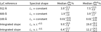
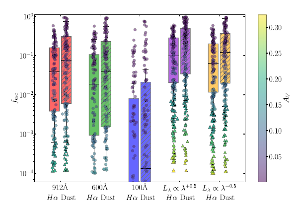
(see Figure A1 and Table 4). Of the flat spectra, a choice of 912 Å as the reference point results in less attenuation overall and thus larger escape fractions. Chisholm et al. (Reference Chisholm2018) discusses the significance of dust attenuation at 912 Å in reference to an idealised model similar to this one, and it is a frequent generous choice to use the Lyman limit as a reference point for LyC escape calculations (Steidel et al. Reference Steidel, Pettini and Adelberger2001; Cooke et al. Reference Cooke, Ryan-Weber, Garel and Díaz2014). Siana et al. (Reference Siana2007) notes the ionising emissions of young stars in stellar population synthesis modelling (Smith et al. Reference Smith, Norris and Crowther2002) do not significantly evolve between the commonly referenced 900 Å range and their chosen 700 Å where the most significant drop-off is below 500 Å. We find that using a 912 Å reference point increases the median calculated escape fraction
 $f{_{\rm esc}^{{\rm H}\alpha}}$
, from 1.9% to 3.9% and has a wider overall range of values. We also find that choosing the lower integration limit of 100 Å brings the median
 $f{_{\rm esc}^{{\rm H}\alpha}}$
only slightly above the chosen threshold, as the attenuation by this wavelength is notably strong.
Median
 $\pm$
IQR escape fractions obtained under different assumptions for the intrinsic LyC spectrum using the common sample described in Figure A1. The
 $f_\mathrm{esc}^{\mathrm{H}\alpha}$
and
 $f_\mathrm{esc}^\mathrm{dust}$
values represent the medians and IQRs of the distributions shown in Figure A1.

Table A1. Long description
A table with four rows and three columns comparing median and interquartile range (IQR) escape fractions under different assumptions for the intrinsic Lyman continuum (LyC) spectrum. The columns are labeled ‘LyC reference’, ‘Spectral shape’, ‘Median %’, and ‘Median %’. The rows are labeled with different LyC references: 912 Å, 600 Å, 100 Å, Integrated slope, and Integrated slope. Each row provides the median and IQR escape fractions for the given LyC reference and spectral shape. The table shows variations in escape fractions based on different assumptions for the intrinsic LyC spectrum.
The LyC dust attenuation approximation comparison. From left to right, the panels show the derived
 $f_{\mathrm{esc}}^{{\rm H}\alpha}$
(plain) and
 $f_{\mathrm{esc}}^{\mathrm{dust}}$
(crosshatched) escape fractions for different assumptions about the intrinsic LyC spectrum. The distributions are calculated using a common sample selected by the
 $L_\lambda$
flat spectrum evaluated at 600 Å with
 $f_{\mathrm{esc}}\gt 10^{-4}$
(0.01%), ensuring a consistent population comparison between attenuation prescriptions. The first three cases assume a flat
 $L_\lambda$
spectrum evaluated at 912, 600 and 100 Å, while the final two adopt power-law spectra with
 $L_\lambda\propto\lambda^{+0.5}$
and
 $L_\lambda\propto\lambda^{-0.5}$
, respectively. Boxes show standard Tukey statistics (25–75th percentile range, median line, and 1.5
 $\times$
IQR whiskers), while individual galaxies are shown as circles coloured by their
 $A_V$
. Galaxies excluded from the common sample that re-enter the detectable regime (
 $\,f_{\mathrm{esc}}\gt 10^{-4}$
) under alternative LyC spectral assumptions are shown as triangles. The corresponding medians and percentile ranges are reported in Table A1.

Integrating the LyC attenuation over a finite wavelength range requires an assumption about the intrinsic spectral shape below the Lyman limit. Power-law approximations are commonly adopted in ionising background models, with spectra such as
 $L_\nu \propto \nu^{-1.5}$
used for AGN and quasar continua (Haardt & Madau Reference Haardt and Madau1996), corresponding to
 $L_\lambda \propto \lambda^{-0.5}$
. We additionally test both this commonly adopted slope and a redder
 $L_\lambda \propto \lambda^{+0.5}$
prescription. In both cases, the resulting median
 $f{_{\rm esc}^{{\rm H}\alpha}}$
values exceed those derived using the flat 912 Å, approximation. Since the flat spectrum normalised at 912 Å, provides the least attenuated possible estimate within our wavelength range, these steeper spectral assumptions produce escape fractions beyond the expected upper limit of this approximation. We therefore consider them unlikely to provide a physically representative description of the intrinsic LyC spectrum for our sample. Although the intrinsic LyC spectrum is expected to depend on the underlying stellar population properties, we find that the flat spectral assumption introduces only limited systematic variation in the derived escape fractions compared with alternative power-law prescriptions. A full treatment would require coupling the attenuation calculation with a stellar population synthesis model.


 α
 α

 α
 α
 χ2
 ξionHII
 α
 ξionHII
 σ

 z=2
 HαModel−HαHα>+2

 [OIII]5007
 Hα
 HαModel−HαHα>+2
 ∼

 ξionHII
 UV
 ξionHII
 ∗
 ξionHII
 ξionHII
 χ2
 ξionHII
 ξion
 −1
 fesc
 ξion
 fesc

 ξionHII
 α
 ξionHII
 χ2
 ξionHII
 ρ
 α
 ρ

 α
 α
 χ2
 z<10.5
 z>10.5
 fesc
 z∼2
 fescβ
 fescModel

 fesc
 fescβ
 fescHα
 ξionHII
 fescHα
 fescHα
 <
 1.5×10⁻⁶
 fescHα>1%
 fescHα=0.1%
 fescHα=0.01%
 ρ
 fescHα
 >

 MUV
 fesc
 fescHα
 fescHα
 <
 1.5×10⁻⁶
 fescHα>1%
 fescHα=0.1%
 fescHα=0.01%,
 MUV=−19
 z=4−6
 fescHα
 MUV
 ρ>0.22
 MUV

 fescHα
 fescHα
 fescHα
 fescHα
 <
 1.5×10⁻⁶
 fescHα>1%
 fescHα=0.1%
 fescHα=0.01%

 [OIII]5007λA˚
 HαA˚
 fescHα
 fescHα
 <1.5×10⁻⁶
 fescHα>1%
 fescHα=0.1%
 fescHα=0.01%
 [OIII]5007λA˚
 HαA˚
 ±
 fescHα
 fescdust
 fescHα
 fescdust
 Lλ
 fesc>10−4
 Lλ
 Lλ∝λ+0.5
 Lλ∝λ−0.5
 ×
 AV
 fesc>10−4

 Open access

