
1 Introduction
Turbulent combustion is a complex, multi-scale phenomenon. Combustion involves a large number of chemical reactions between numerous species with different transport properties. The conversion of the enthalpy of formation to sensible enthalpy affects the flow field through changes in temperature, density, viscosity and pressure. The turbulent flow field involves complex chaotic yet correlated motions. These motions induce stretch and other unsteady effects on the flame: the thin region characterized by strong thermal and species transport and heat release due to chemical reactions. Understanding these complex turbulence–flame interactions is difficult and far from complete. One cannot overemphasize the importance of developing models to understand and predict these interactions. They are essential for designing and improving the efficiency of propulsion and energy conversion devices, taming combustion instabilities, reducing emissions and also to explain many naturally occurring combustion processes. The rate at which a turbulent premixed flame propagates on average is one of the most important quantities, although yet to be satisfactorily understood and accurately modelled.
For a freely propagating, unstretched, adiabatic, planar premixed flame, also known as the standard premixed flame, the laminar flame speed conditioned on the unburnt side,  $S_{L}$, is a crucial parameter (Law Reference Law2006). One can obtain
 $S_{L}$ by analysing the thermal and the chemical structure of this standard premixed flame. Using the single-step reaction mechanism and large activation energy assumption, we know that, in the preheat zone of the flame, convection and diffusion processes balance, while in the reaction zone, diffusion and reactions dominate and balance one another. For practical utility, the experimentally obtained
 $S_{L}$ is routinely used to validate chemical reaction mechanisms (Law Reference Law2006). However, for unsteady, multi-dimensional configurations, inherent to turbulent reacting flows of engineering relevance, it is difficult to define a flame speed as uniquely as
 $S_{L}$. Multiple definitions, such as the local consumption speed
 $S_{c}$ and flame displacement speed
 $S_{d}$, exist. For a standard premixed flame these different definitions are equivalent to
 $S_{L}$, but they need not be equal in turbulent premixed flames. Therefore, evaluating the local flame speed for a turbulent flame requires careful consideration of numerous parameters, depending on the application and analysis (Lipatnikov & Chomiak Reference Lipatnikov and Chomiak2005; Driscoll Reference Driscoll2008). Additionally, among the myriad manifestations of complex turbulent–flame interactions, the variation of both the flame speeds is a common observation. The flame speeds significantly vary in time and even spatially over an isoscalar surface, say over an isotherm, inside a flame.
An important parameter relevant to turbulent premixed flames is  $S_{d}$. It is the speed with which a point with position vector
 $\boldsymbol{x}^{F}$ on a flame surface moves along the local normal
 $\boldsymbol{n}^{F}$ of the flame surface relative to the local fluid velocity
 $\boldsymbol{u}^{F}$. The equation below expresses the mathematical relationship among these quantities.
 $$\begin{eqnarray}\frac{\text{d}}{\text{d}t}\boldsymbol{x}^{F}(t)=\boldsymbol{u}^{F}(t)+S_{d}^{F}(t)\boldsymbol{n}^{F}(t),\end{eqnarray}$$
where  $\boldsymbol{v}^{F}=\text{d}\boldsymbol{x}^{F}(t)/\text{d}t$ is the absolute velocity of a point on the flame surface with respect to a fixed observer and
 $t$ denotes time. We have oriented
 $\boldsymbol{n}^{F}$ such that it points toward the fresh reactants. Thus, positively curved surfaces are curved convex to fresh reactants while negatively curved surfaces are curved concavely to fresh reactants. We will explain the importance of the superscript
 $F$ later, in the context of flame particle tracking.
The parameter  $S_{d}$ is crucial in models based on flame-front tracking methods (Peters Reference Peters2000; Veynante & Vervisch Reference Veynante and Vervisch2002; Poinsot & Veynante Reference Poinsot and Veynante2005), such as the level-set method, and models based on flame surface density (FSD) formalisms (Trouvé & Poinsot Reference Trouvé and Poinsot1994; Veynante & Vervisch Reference Veynante and Vervisch2002). One can easily derive the level-set equation, or the G-equation, by using the constraint that the time derivative of the level-set value of the level-set surface does not change as one moves with its absolute velocity
 $\boldsymbol{v}=\boldsymbol{u}+S_{d}\boldsymbol{n}$. Equation (1.2) shows the G-equation (Williams Reference Williams1985; Kerstein, Ashurst & Williams Reference Kerstein, Ashurst and Williams1988). In FSD-based models,
 $S_{d}$ appears in the transport equation for the flame surface density
 $\unicode[STIX]{x1D6F4}$ using which one subsequently evaluates the mean reaction rate. Equation (1.3) shows the transport equation for
 $\unicode[STIX]{x1D6F4}$, where
 $K$ is the stretch rate and
 $\langle \;\rangle _{s}$ denotes an area-weighted average. Clearly, a model for the flame displacement speed is required to solve these equations. Unfortunately,
 $S_{d}$ can vary widely over and within the flame, depending on the local physico-chemical state. To our knowledge, there is no complete model of
 $S_{d}$ for turbulent premixed flames.
 $$\begin{eqnarray}\displaystyle & \displaystyle \frac{\unicode[STIX]{x2202}G}{\unicode[STIX]{x2202}t}+\boldsymbol{u}\boldsymbol{\cdot }\unicode[STIX]{x1D735}G=S_{d}|\unicode[STIX]{x1D735}G|, & \displaystyle\end{eqnarray}$$
 $$\begin{eqnarray}\displaystyle & \displaystyle \frac{\unicode[STIX]{x2202}\unicode[STIX]{x1D6F4}}{\unicode[STIX]{x2202}t}+\unicode[STIX]{x1D735}\boldsymbol{\cdot }\langle \boldsymbol{u}+S_{d}\boldsymbol{n}\rangle _{s}\unicode[STIX]{x1D6F4}=\langle K\rangle _{s}\unicode[STIX]{x1D6F4}. & \displaystyle\end{eqnarray}$$
With the advent of high-performance computing, large-eddy simulations (LES) are becoming the technique of choice for simulating turbulent reacting flows of practical relevance. Developing robust and versatile models for  $S_{d}$, therefore, has a strong bearing on making simulations of turbulent premixed flames convenient and computationally less intensive, allowing turbulent combustion simulations at very high, engine relevant, Reynolds numbers. Moreover, once suitable models are developed for the local
 $S_{d}$, the predictions from those models can also be used to determine the turbulent flame speed
 $S_{T}$ which is an averaged, global quantity. Determination of
 $S_{T}$ is useful for understanding flame stabilization of turbulent premixed flames and evaluating the mean fuel consumption rate.
An important feature of turbulent premixed flames is the wide distribution of the flame displacement speed  $S_{d}$. The wide scatter of
 $S_{d}$ with respect to non-dimensional stretch rate has been reported by Chen & Im (Reference Chen and Im1998, Reference Chen and Im2000) for turbulent premixed methane–air and hydrogen–air flames. Subsequently, Hawkes & Chen (Reference Hawkes and Chen2005) evaluated models for flame stretch due to curvature in the thin reaction zones and stated that ‘while most flame area has a small curvature, most stretch occurs for a large curvature. This implies that steady and/or small curvature models are unlikely to be successful for modelling the stretch response of premixed flame’. Then, Chakraborty, Klein & Cant (Reference Chakraborty, Klein and Cant2007) evaluated the effects of stretch rate on displacement speed in turbulent premixed flame kernels in the thin reaction-zone regime and commented that ‘there remains a need to model the curvature response of the combined reaction and normal diffusion components of
 $S_{d}$ to account properly for curvature stretch effects’. Recently, Im et al. (Reference Im, Arias, Chaudhuri and Uranakara2016) reviewed the magnitude of the excursions of local
 $S_{d}$ away from
 $S_{L}$ and questioned whether the flame speed flame stretch
 $S_{d}-K$ relations based on laminar flame theory could address these large excursions. Im et al. (Reference Im, Arias, Chaudhuri and Uranakara2016) emphasized the need to understand the large excursions of local
 $S_{d}$ for turbulent premixed flames. It will be shown in this paper that, in some parts of the turbulent flame, the stretch rate based laminar flame theory is valid, and in other parts it is not. Before we address these interesting behaviours and modelling aspects of
 $S_{d}$ in a turbulent premixed flame, we first briefly review how laminar flame speed models have evolved over the last eight decades.
Darrieus (Reference Darrieus1938) and Landau (Reference Landau1944), independently, used a constant flame speed model to understand the stability of a planar premixed flame. The flame was represented by a structureless interface on which each point propagated with the constant flame speed  $S_{L}$. Under these assumptions, a premixed flame is unconditionally unstable. Markstein (Reference Markstein1964) incorporated the effect of flame surface curvature with the help of a phenomenological coefficient. Asymptotic studies (Matalon & Matkowsky Reference Matalon and Matkowsky1982; Pelce & Clavin Reference Pelce and Clavin1982; Frankel & Sivashinsky Reference Frankel and Sivashinsky1983) exploited the large difference in the hydrodynamic length scale
 $L$ and the diffusion length scale of the flame
 $\ell _{f}=\unicode[STIX]{x1D6FC}_{u}/S_{L}$, i.e.
 $L\gg \ell _{f}$, and showed that
 $S_{d}$ is not only dependent on curvature, as envisaged by Markstein, but also on the strain rates in the flow field;
 $\unicode[STIX]{x1D6FC}_{u}$ is the thermal diffusivity of the fresh reactant mixture. Within the weak-stretch limit, the strain-rate and curvature effects combine, and the stretch rate
 $K$ emerges as the sole parameter. In this weak-stretch limit,
 $S_{d}$ is a linear function of
 $K$. Equation (1.4) expresses this linear relationship.
 $$\begin{eqnarray}S_{d}=S_{L}-{\mathcal{L}}K.\end{eqnarray}$$
The proportionality constant,  ${\mathcal{L}}$, called the Markstein length, measures the sensitivity of the flame speed to
 $K$. It can be positive, negative or zero depending on the mixture composition. It captures the altered transport and reaction rates within a flame due to the presence of external stretch rates. On the other hand, under the steady-state assumption suitable for a slowly varying flame and using integral analysis, Sun & Law (Reference Sun and Law2000) and Law (Reference Law2006) showed that the non-dimensional mass flux on the unburned side
 $\tilde{f}_{u}=f_{u}/f^{0}$ for a stretched planar flame varies nonlinearly with a factor
 $\unicode[STIX]{x1D70E}^{0}$;
 $f^{0}$ is the mass flux for a standard premixed flame and
 $\unicode[STIX]{x1D70E}^{0}=Ma^{0}Ka^{0}$, where
 $Ma^{0}$ is a Markstein number (non-dimensional Markstein length) and
 $Ka^{0}=(\ell _{f}/S_{L})K$ is the non-dimensional stretch rate (see Law (Reference Law2006)). Equation (1.5) expresses the nonlinear model between
 $\tilde{f}_{u}$ and
 $\unicode[STIX]{x1D70E}^{0}$.
 $$\begin{eqnarray}\tilde{f}_{u}^{2}\ln \tilde{f}_{u}^{2}=2\unicode[STIX]{x1D70E}^{0}.\end{eqnarray}$$
An important outcome, within the assumptions of (1.4) and (1.5), is that  $S_{d}$ is only a function of parameter
 $K$. Therefore, different flames with the same value of
 $K$ should behave identically, irrespective of the geometry or flame configuration – planar counter-flow flames, spherically expanding flames, Bunsen flames, etc. This simplification enables one to choose simple prototypes or canonical geometries as representative of more complex turbulent flames (Poinsot, Echekki & Mungal Reference Poinsot, Echekki and Mungal1992). Even in experiments, one evaluates the flame speed at different values of
 $K$. Then, using (1.4), one obtains
 $S_{L}$ through extrapolation (Wu & Law Reference Wu and Law1985; Law Reference Law2006). Thus, due to its simplicity, (1.4) is an important relationship in combustion studies. This has motivated efforts to obtain theoretical expressions for
 ${\mathcal{L}}$ using the integral (Chung & Law Reference Chung and Law1988; de Goey & ten Thije Boonkkamp Reference de Goey and ten Thije Boonkkamp2008) or asymptotic (Matalon & Matkowsky Reference Matalon and Matkowsky1982; Pelce & Clavin Reference Pelce and Clavin1982; Frankel & Sivashinsky Reference Frankel and Sivashinsky1983; Giannakopoulos et al. Reference Giannakopoulos, Gatzoulis, Frouzakis, Matalon and Tomboulides2015) approaches. A large number of numerical (Echekki & Chen Reference Echekki and Chen1996; Chen & Im Reference Chen and Im1998, Reference Chen and Im2000; Chakraborty et al. Reference Chakraborty, Klein and Cant2007) and experimental studies are also performed to determine values of
 ${\mathcal{L}}$ for different chemical mixtures using different flame configurations.
When Bechtold & Matalon (Reference Bechtold and Matalon2001) assessed the effect of stoichiometry and accounted for the variation in mass flux within the flame zone, they found that two distinct Markstein lengths are important, unlike (1.4). Also, when Clavin & Graña-Otero (Reference Clavin and Graña-Otero2011) replaced the assumption of a single-step global reaction by multi-step mechanisms, they also found that two Markstein lengths emerge for characterizing the effect of stretch rate and curvature. Flames are finitely thick, and in experiments and numerical simulations which resolve the flame thickness, one often faces the dilemma of choosing an appropriate surface to represent the flame. The recent work of Giannakopoulos et al. (Reference Giannakopoulos, Gatzoulis, Frouzakis, Matalon and Tomboulides2015) addresses this issue in the context of flame speed modelling. In the weak-stretch limit, they have derived a model for the density-weighted flame displacement speed  $\widetilde{S_{d}}=\unicode[STIX]{x1D70C}S_{d}/\unicode[STIX]{x1D70C}_{u}$ for an isotherm within the preheat zone. Density is denoted by
 $\unicode[STIX]{x1D70C}$ and
 $\unicode[STIX]{x1D70C}_{u}$ is the density of the fresh reactants. Even in their work, two Markstein lengths, stretch Markstein length
 ${\mathcal{L}}_{K}$ and curvature Markstein length
 ${\mathcal{L}}_{\unicode[STIX]{x1D705}}$, emerge. Equation (1.6) below expresses the model proposed by Giannakopoulos et al. (Reference Giannakopoulos, Gatzoulis, Frouzakis, Matalon and Tomboulides2015). Unlike (1.4), (1.6) has two variables – stretch rate
 $K$ and curvature
 $\unicode[STIX]{x1D705}$ – that feature in the model;
 $\unicode[STIX]{x1D705}$ is the total curvature which is the sum of the principal curvatures
 $\unicode[STIX]{x1D705}_{1}$ and
 $\unicode[STIX]{x1D705}_{2}$.
 $$\begin{eqnarray}\widetilde{S_{d}}(\unicode[STIX]{x1D703}^{\ast })=S_{L}-{\mathcal{L}}_{K}(\unicode[STIX]{x1D703}^{\ast })K-{\mathcal{L}}_{\unicode[STIX]{x1D705}}(\unicode[STIX]{x1D703}^{\ast })S_{L}\unicode[STIX]{x1D705}.\end{eqnarray}$$
The Markstein lengths  ${\mathcal{L}}_{K}$ and
 ${\mathcal{L}}_{\unicode[STIX]{x1D705}}$ are functions of the non-dimensional temperature
 $\unicode[STIX]{x1D703}^{\ast }=T_{0}/T_{u}$ and many other variables, as shown below;
 $T_{0}$ is the level-set value of temperature and
 $T_{u}$ is the temperature of the fresh reactants. The above expression reveals that, to the leading order,
 $\widetilde{S_{d}}$ evaluated on an isotherm representing the flame front is equal to
 $S_{L}$. A first-order correction due to the response of the flame to the stretch rate is given by
 ${\mathcal{L}}_{K}K$ while
 ${\mathcal{L}}_{\unicode[STIX]{x1D705}}S_{L}\unicode[STIX]{x1D705}$ is another correction due to the location of the isotherm within the preheat zone. Equations (1.7) and (1.8) show how one can calculate the Markstein lengths for a given mixture (see Giannakopoulos et al. Reference Giannakopoulos, Gatzoulis, Frouzakis, Matalon and Tomboulides2015).
 $$\begin{eqnarray}\displaystyle & \displaystyle {\mathcal{L}}_{K}=\ell _{f}\left(\unicode[STIX]{x1D6E4}-\int _{1}^{\unicode[STIX]{x1D703}^{\ast }}\frac{\unicode[STIX]{x1D706}(x)}{x}\,\text{d}x-\int _{\unicode[STIX]{x1D703}^{\ast }}^{\unicode[STIX]{x1D70E}}\frac{\unicode[STIX]{x1D706}(x)}{x-1}\,\text{d}x\right), & \displaystyle\end{eqnarray}$$
 $$\begin{eqnarray}\displaystyle & \displaystyle {\mathcal{L}}_{\unicode[STIX]{x1D705}}=\ell _{f}\int _{\unicode[STIX]{x1D703}^{\ast }}^{\unicode[STIX]{x1D70E}}\frac{\unicode[STIX]{x1D706}(x)}{x-1}\,\text{d}x, & \displaystyle\end{eqnarray}$$
where the expression for  $\unicode[STIX]{x1D6E4}$ is given by
 $$\begin{eqnarray}\unicode[STIX]{x1D6E4}=\frac{\unicode[STIX]{x1D70E}}{\unicode[STIX]{x1D70E}-1}\int _{1}^{\unicode[STIX]{x1D70E}}\frac{\unicode[STIX]{x1D706}(x)}{x}\,\text{d}x+\frac{\unicode[STIX]{x1D6FD}(Le_{eff}-1)}{2(\unicode[STIX]{x1D70E}-1)}\int _{1}^{\unicode[STIX]{x1D70E}}\ln \left(\frac{\unicode[STIX]{x1D70E}-1}{x-1}\right)\frac{\unicode[STIX]{x1D706}(x)}{x}\,\text{d}x.\end{eqnarray}$$
In these equations,  $\ell _{f}$ is the diffusion thickness of the flame;
 $\unicode[STIX]{x1D706}$ is the thermal conductivity of the mixture normalized by its value on the reactant side;
 $\unicode[STIX]{x1D706}\sim (T/T_{u})^{a}$ approximates the variation of thermal properties with temperature, where
 $a$ is the power-law exponent;
 $\unicode[STIX]{x1D70E}=\unicode[STIX]{x1D70C}_{u}/\unicode[STIX]{x1D70C}_{b}$ is the thermal expansion factor. For subsonic flames, where the pressure is nearly uniform
 $\unicode[STIX]{x1D70C}\sim 1/T$, therefore,
 $\unicode[STIX]{x1D70E}\approx T_{b}/T_{u}$, where
 $T_{b}$ is the temperature of the products;
 $\unicode[STIX]{x1D6FD}$ is the Zeldovich number and
 $Le_{eff}$ is the effective Lewis number of the mixture. The above equations show that
 ${\mathcal{L}}_{K}$ is a function of the Lewis number;
 $Le_{eff}$ is given by the following equation (see Matalon, Cui & Bechtold Reference Matalon, Cui and Bechtold2003). Here,
 $Le_{F}$ and
 $Le_{O}$ are the limiting Lewis numbers for the lean and rich conditions, respectively, near the flammability limits.
 $$\begin{eqnarray}\displaystyle Le_{eff}=\left\{\begin{array}{@{}ll@{}}\displaystyle \frac{Le_{O}+{\mathcal{A}}Le_{F}}{1+{\mathcal{A}}}\quad & \unicode[STIX]{x1D719}<1,\\ \displaystyle \frac{Le_{F}+{\mathcal{A}}Le_{O}}{1+{\mathcal{A}}}\quad & \unicode[STIX]{x1D719}>1,\end{array}\right. & & \displaystyle\end{eqnarray}$$
where  $\unicode[STIX]{x1D719}$ is the equivalence ratio and
 $$\begin{eqnarray}\displaystyle {\mathcal{A}}=\left\{\begin{array}{@{}ll@{}}1+\unicode[STIX]{x1D6FD}(\unicode[STIX]{x1D719}^{-1}-1)\quad & \unicode[STIX]{x1D719}<1,\\ 1+\unicode[STIX]{x1D6FD}(\unicode[STIX]{x1D719}-1)\quad & \unicode[STIX]{x1D719}>1.\end{array}\right. & & \displaystyle\end{eqnarray}$$
When we evaluate  $S_{d}$ from direct numerical simulation (DNS) to compare it with the predictions from the models, the expression for
 $S_{d}$ depends on the scalar we use to identify the isoscalar surface that represents the flame. Equations (1.12) and (1.13) show the expressions of
 $S_{d}$ for an isotherm and for a surface of constant mass fraction of a
 $k$th species,
 $Y_{k}$, respectively. In this study, we use isotherms to represent a premixed flame and therefore use the expression for
 $S_{d,T}$ to evaluate
 $S_{d}$ from the DNS databases.
 $$\begin{eqnarray}\displaystyle & \displaystyle S_{d,T}=\frac{1}{\unicode[STIX]{x1D70C}C_{p}|\unicode[STIX]{x1D735}T|}\left[\unicode[STIX]{x1D735}\boldsymbol{\cdot }(\unicode[STIX]{x1D706}^{\prime }\unicode[STIX]{x1D735}T)+\unicode[STIX]{x1D70C}\unicode[STIX]{x1D735}T\cdot \mathop{\sum }_{k}({\mathcal{D}}_{k}C_{p,k}\unicode[STIX]{x1D735}Y_{k})-\mathop{\sum }_{k}h_{k}\dot{\unicode[STIX]{x1D714}}_{k}\right], & \displaystyle\end{eqnarray}$$
 $$\begin{eqnarray}\displaystyle & \displaystyle S_{d,Y}=\frac{1}{\unicode[STIX]{x1D70C}|\unicode[STIX]{x1D735}Y_{k}|}[\unicode[STIX]{x1D735}\boldsymbol{\cdot }(\unicode[STIX]{x1D70C}{\mathcal{D}}_{k}\unicode[STIX]{x1D735}Y_{k})+\dot{\unicode[STIX]{x1D714}}_{k}]. & \displaystyle\end{eqnarray}$$
Here  $C_{p}$ is the mixture-averaged mass-specific heat capacity, whereas
 $C_{p,k}$ is the mass-specific heat capacity for the
 $k$th species;
 ${\mathcal{D}}_{k}$ is the mass diffusivity,
 $h_{k}$ is the enthalpy and
 $\dot{\unicode[STIX]{x1D714}}_{k}$ is the net mass-production rate for the
 $k$th species;
 $\unicode[STIX]{x1D706}^{\prime }$ is the thermal conductivity of the mixture.
Giannakopoulos et al. (Reference Giannakopoulos, Gatzoulis, Frouzakis, Matalon and Tomboulides2015) validated the results from asymptotic analysis (1.6)–(1.9) with numerical simulations of outwardly propagating and point-source stabilized spherical flames using single-step as well as detailed reaction mechanisms over a range of equivalence ratios for propane–air mixtures. Recently, using numerical and experimental set-ups of an axisymmetric vortex interacting with a laminar premixed flame, Thiesset et al. (Reference Thiesset, Halter, Bariki, Lapeyre, Chauveau, Gökalp, Selle and Poinsot2017) demonstrated the importance of the two Markstein lengths. However, they argued that the ‘laminar’ Markstein lengths (1.7) and (1.8) are inadequate in explaining the complete flame response. While these two studies are useful, they do not assess the role of the Markstein lengths in understanding and modelling  $S_{d}$ for turbulent premixed flames. Efforts to study the applicability of the Markstein length models to understand turbulent premixed flames are common. For example, Creta & Matalon (Reference Creta and Matalon2011) and Fogla, Creta & Matalon (Reference Fogla, Creta and Matalon2017) assessed the role of integral length scale, hydrodynamic instability, etc., on the turbulent flame speed. However, these studies did not resolve the flame thickness and represented the flame as a surface. Consequently, only one Markstein length was required. Thus, despite these numerous studies, there is a pressing need to assess the role of the two-parameter Markstein length model by Giannakopoulos et al. (Reference Giannakopoulos, Gatzoulis, Frouzakis, Matalon and Tomboulides2015) inspired from the original model by Bechtold & Matalon (Reference Bechtold and Matalon2001), for understanding and modelling
 $S_{d}$ in turbulent premixed flames. This objective forms one of the central themes of this study.
This work deals with the local description of turbulent premixed flames. With the help of DNS, we simulate turbulent premixed flames of  $\text{H}_{2}$–air mixtures in the thin reaction regime. To use a large hydrocarbon as a fuel, the reaction mechanism must be reduced to ensure feasibility of the reacting flow DNS. However, a
 $\text{H}_{2}$–air mixture allows implementation of a detailed reaction mechanism, ensuring that the DNS remains free from any possible implication of reaction mechanism reduction. In this study, the DNS databases correspond to a moderate Karlovitz number of
 $O(10)$.
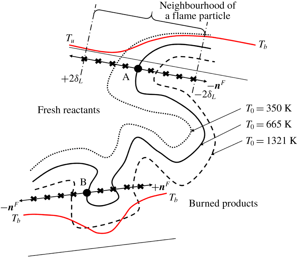
To understand the propagation characteristics of flame surfaces locally, we have used the concept of flame particles. A flame particle is a hypothetical point co-moving with a reacting isoscalar surface. Flame particles are thus a class of surface points, a concept introduced by Pope (Reference Pope1988), and provide a local description of the evolution of flame surfaces in turbulence. In other words, an ensemble of flame particles forms a flame surface, and an ensemble of flame surfaces forms a premixed flame. Equation (1.1) is the governing equation for the flame particle position  $\boldsymbol{x}^{F}$. A flame particle is principally different from a fluid particle. While a fluid particle, theoretically, has an infinite lifetime, a flame particle has a finite lifetime (Chaudhuri Reference Chaudhuri2015). Also, while a fluid particle follows the local flow, a flame particle follows the local flame surface. Using flame particle tracking (FPT), one can trace trajectories of flame particles on any isoscalar surface representing the premixed flame. Chaudhuri (Reference Chaudhuri2015) developed the FPT algorithm to trace trajectories of flame particles forward in time. Uranakara et al. (Reference Uranakara, Chaudhuri, Dave, Arias and Im2016) used this tool to gather spatio-temporal details of relevant parameters at flame particle positions and investigated the primary factors that influence the
 $S_{d}$ at these locations. Recently, Dave, Abinesh & Chaudhuri (Reference Dave, Abinesh and Chaudhuri2018) extended the tracking algorithm to track the position of flame particles backward in time. This tool is called the backward flame particle tracking (BFPT) algorithm. This study showed that multiple clusters of leading points, the points on a flame surface which are spatially most advanced and positively curved towards the fresh reactants, generate the complete turbulent flame surface after a finite time.
In this study, we refer to the FPT algorithm developed by Chaudhuri (Reference Chaudhuri2015) as forward flame particle tracking (FFPT), to distinguish it from BFPT. Starting with a uniform distribution of flame particles spanning a complete isotherm, application of BFPT leads to formation of multiple clusters of the flame particles in the leading regions of the corresponding isotherm, at an earlier time. These leading regions, therefore, serve as the generation locations of the isotherm. Subsequently, applying FFPT, we can trace the trajectories of flame particles from these generation locations at the leading points to their final annihilation at the negatively curved trailing regions of the flame surface. During evolution, the flame particles obviously spread over the entire flame surface at some intermediate time instant. At this instant, the statistics of the ensemble of the flame particles closely approximate the statistics over the entire flame surface. Therefore, tracking flame particles from their generation locations to annihilation locations gives us the opportunity to study the complete lifetime of local flame surface elements. In other words, after the turbulent flame has achieved statistical stationarity, if we study a large number of such flame particles over their complete lifetimes and record all their states, a manifold of such states is created which can represent any possible state realizable from the turbulent flame with the same inlet and ambient conditions. This is because any instantaneously realizable local state from the flame must belong to some flame particle (which need not belong to those recorded) that is somewhere at or in between its generation and annihilation states. With all possible states accessible in the time, in this study, first, we assess the applicability of the two-parameter Markstein length model (1.6) locally, along the trajectories of flame particles. The unique advantages of such a Lagrangian investigation is that it provides the context and the natural requirement that lead to the emergence of two different models for  $S_{d}$. These advantages will also be elucidated.
We present this paper as follows. Following the Introduction, we discuss the DNS databases and the tracking methodologies for flame particles, both in forward time (FFPT) and in backward time (BFPT). The subsequent section is Results and Discussion. We have organized this section into four major subsections. Subsequently, we discuss the implications of the findings of this study, followed by Conclusions.
2 Computational methodologies
In this study, first, we have performed DNS of turbulent premixed flames and saved the snapshots of the Eulerian fields at a time interval which is a fraction of the Kolmogorov time scale. Subsequently, we used these fields, along with the flame particle tracking tools, to trace the trajectories of the flame particles. This section presents the details of these computational methods.
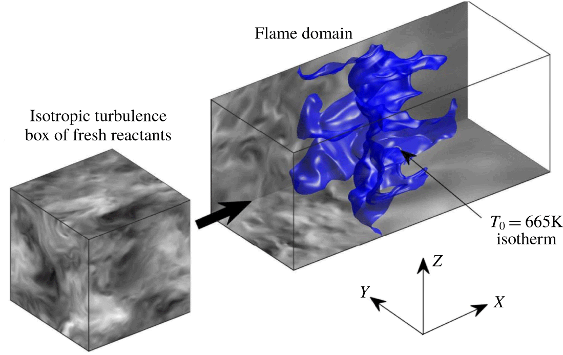
A schematic showing the set-up of the DNS of statistically planar flames performed in this study. It shows the two essential steps for the DNS: simulation of isotropic turbulence of fresh reactants in a cube and the simulation of a turbulent flame in a cuboid.

2.1 Direct numerical simulations
We have used an open-source solver called the Pencil code to perform the DNS of statistically planar turbulent premixed flames. Babkovskaia, Haugen & Brandenburg (Reference Babkovskaia, Haugen and Brandenburg2011) extended the Pencil code to simulate reacting flows. In the governing equations, the spatial terms are discretized using a sixth-order accurate central difference scheme. However, for convection terms, the use of a fifth-order accurate upwinding scheme helps in removing any spurious oscillations from the field variables. The solution marches in time using a low-storage, third-order accurate Runge–Kutta RK3-2N scheme. For modelling  $\text{H}_{2}$–air chemistry, we used a detailed reaction mechanism of nine species and 21 reactions proposed by Li et al. (Reference Li, Zhao, Kazakov and Dryer2004).
The DNS involves two steps. Figure 1 shows the schematic of the set-up for the problem. First, we simulate a three-dimensional flow field of isotropic turbulence with a reactant mixture in a cube. The reactant mixture corresponds to a particular equivalence ratio  $\unicode[STIX]{x1D719}$ and pressure
 $P$. We prescribe periodic boundary conditions on all the six faces of this cube and inject energy into the flow field by forcing small wavenumbers to balance energy dissipation. The amount of injected energy decides the root mean square of the turbulent fluctuations
 $u_{0}$ in velocity, while the average forcing wavenumber characterizes the integral length scale
 $\ell _{0}$. Once this simulation reaches a statistically stationary state, characterized by the Kolmogorov–Obukhov (KO)
 $-5/3$ scaling law of the energy spectrum, we use the isotropic turbulent field for the subsequent flame simulation. The spatial resolution of the isotropic turbulent flow field is quantified using the parameter
 $k_{max}\unicode[STIX]{x1D702}$. The largest resolvable wavenumber for a given mesh spacing
 $\unicode[STIX]{x1D6E5}_{x}$ is given by
 $k_{max}=\unicode[STIX]{x03C0}/\unicode[STIX]{x1D6E5}_{x}$. The Kolmogorov length scale is
 $\unicode[STIX]{x1D702}=(\unicode[STIX]{x1D708}^{3}/\unicode[STIX]{x1D716})^{1/4}$, where
 $\unicode[STIX]{x1D708}$ is the kinematic viscosity and
 $\unicode[STIX]{x1D716}$ is the mean dissipation rate. For our DNS databases, we have maintained adequate spatial resolution by ensuring
 $k_{max}\unicode[STIX]{x1D702}\geqslant 1.5$ (Yeung & Pope Reference Yeung and Pope1988).
In the second step, we select a cuboid with a desired aspect ratio  $L_{x}/L_{y}$. The length of the cuboid along the streamwise
 $X$ direction is
 $L_{x}$, while
 $L_{y}$ is the length along the lateral
 $Y$ direction. We have used
 $L_{y}=L_{z}$ for all our simulations;
 $N_{x}$,
 $N_{y}$, and
 $N_{z}$ are the number of grid points along the corresponding directions. The cuboid has periodic boundary conditions in the lateral
 $Y$ and
 $Z$ directions and Navier–Stokes characteristic boundary conditions (NSCBC) in the streamwise
 $X$ direction. We initialize computations in this cuboid with a planar laminar flame at an appropriate distance downstream of the inlet
 $Y$–
 $Z$ plane. For an adequate resolution of the premixed flame, we ensure that
 $\unicode[STIX]{x1D6FF}_{L}/\unicode[STIX]{x1D6E5}_{x}\approx 18$, where
 $\unicode[STIX]{x1D6FF}_{L}=(T_{b}-T_{u})/(\text{d}T/\text{d}x_{max})$ is the thermal thickness of the standard premixed flame. Then, the isotropic turbulent flow field, simulated in the first step, issues from the inlet
 $Y$–
 $Z$ plane of the cuboid after superimposing it with a constant streamwise velocity
 $\overline{\boldsymbol{u}}=\overline{u_{x}}$. It is not adjusted during the simulation but is fixed by trial and error to a value such that the entire turbulent flame brush remains within the computational domain. The turbulent flow field of the reactant mixture travels downstream and interacts with the planar laminar flame. Due to these flow–flame interactions, the flame is stretched and folded at a multitude of length scales and time scales. To characterize the flame simulations, we have calculated the Karlovitz (
 $Ka$) and the Damköhler (
 $Da$) numbers;
 $Da=\unicode[STIX]{x1D70F}_{0}/\unicode[STIX]{x1D70F}_{f}$ is the ratio of integral time scale
 $\unicode[STIX]{x1D70F}_{0}=\ell _{0}/u_{0}$ from the isotropic cube with respect to the flame time scale
 $\unicode[STIX]{x1D70F}_{f}=\unicode[STIX]{x1D6FF}_{L}/S_{L}$, while
 $Ka=\unicode[STIX]{x1D70F}_{f}/\unicode[STIX]{x1D70F}_{\unicode[STIX]{x1D702}}$ is the ratio of the flame time scale with respect to the smallest time scales in the unburned mixture – the Kolmogorov time scale
 $\unicode[STIX]{x1D70F}_{\unicode[STIX]{x1D702}}$. For our simulations,
 $Da>1$ and
 $Ka>1$. Therefore, the DNS databases correspond to the thin reaction-zone regime. The flow–flame interactions begin around one
 $\unicode[STIX]{x1D70F}_{0}$ after the start of the simulation and we allow this interaction to go on for at least one more
 $\unicode[STIX]{x1D70F}_{0}$ i.e. at least
 $2\unicode[STIX]{x1D70F}_{0}$ from the beginning of the simulation. By
 $t\approx 2\unicode[STIX]{x1D70F}_{0}$ from the beginning of the simulation the flame is adequately wrinkled and from hereon we save the Eulerian snapshots from the DNS at fine time interval
 $\unicode[STIX]{x0394}t$. The DNS data are collected for a duration of a minimum of one
 $\unicode[STIX]{x1D70F}_{0}$ and during this interval the time series of the surface area of the
 $T_{0}=350~\text{K}$ isotherm and the spatial average of
 $Y_{H}$ are nearly statistically steady, indicating that the turbulent premixed flame has reached a statistically steady state. The flame particle tracking algorithms – FFPT and BFPT – use these saved Eulerian DNS fields. To keep the errors at an acceptable level during the flame particle tracking, we ensure
 $\unicode[STIX]{x1D70F}_{\unicode[STIX]{x1D702}}/\unicode[STIX]{x0394}t=O(10)$, i.e. we save the Eulerian fields at a fraction of
 $\unicode[STIX]{x1D70F}_{\unicode[STIX]{x1D702}}$. Table 1 presents the details of the major simulation parameters discussed above, for the two databases presented in this study. Case-L and Case-H denote the databases with lower and higher turbulent Reynolds numbers, respectively. For the
 $\text{H}_{2}$–air mixture with
 $\unicode[STIX]{x1D719}=0.81$,
 $Le_{eff}$ evaluates to 0.93. From the parameters in table 1, it is also evident that the turbulent intensity for both the cases is at least three times
 $S_{L}$. Given the above two facts, we do not expect the flame to exhibit any thermodiffusive or hydrodynamic instability and the stretching and wrinkling of the premixed flame is due to turbulence.
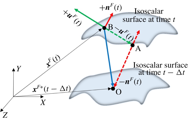
A schematic showing the estimation stage of the BFPT algorithm.

Details of DNS parameters. For all cases,  $T_{u}=310~\text{K}$,
 $P=1~\text{atm}$,
 $\unicode[STIX]{x1D719}=0.81$,
 $L_{y}=L_{z}$,
 $N_{y}=N_{z}$,
 $S_{L}=185~\text{cm}~\text{s}^{-1}$ and
 $\unicode[STIX]{x1D6FF}_{L}=0.036~\text{cm}$.
 $Re_{0}=\ell _{0}u_{0}/\unicode[STIX]{x1D708}$ is the turbulent Reynolds number.

2.2 Forward flame particle tracking
FFPT is a tracking algorithm developed by Chaudhuri (Reference Chaudhuri2015) for Lagrangian analysis of turbulent premixed flames. Using this computational tool, we can trace the trajectories of mathematical points, called flame particles, on any isoscalar surface representing the premixed flame in forward time. FFPT offers a new paradigm for the investigations of turbulence–flame interactions. It is, in principle, different from the fluid particle/parcel tracking widely used in non-reacting turbulence studies and the reacting flow studies of Day et al. (Reference Day, Tachibana, Bell, Lijewski, Beckner and Cheng2012, Reference Day, Tachibana, Bell, Lijewski, Beckner and Cheng2015), Osborne et al. (Reference Osborne, Ramji, Carter and Steinberg2017) and Hamlington et al. (Reference Hamlington, Darragh, Briner, Towery, Taylor and Poludnenko2017). Sometimes, the fluid parcels can be complex fluid-dynamic strain-rate structures of the turbulent flow field (Steinberg & Driscoll Reference Steinberg and Driscoll2009). Equation (1.1) is the governing equation for the position  $\boldsymbol{x}^{F}$ of a flame particle. To differentiate Lagrangian parameters evaluated at the flame particle’s position from the Eulerian variables, we use a superscript
 $F$. In the FFPT algorithm, to solve the discretized form of (1.1) the triangle-ray intersection algorithm by Möller & Trumbore (Reference Möller and Trumbore2005) is used. FFPT usually starts with a uniform distribution of flame particles on a flame surface. As time progresses, the flame particles cluster in the negatively curved trailing regions of the flame and annihilate. Hence, in the earlier works, FFPT provided flame particle trajectories for only a fraction of their total lifetime. Interested readers can refer to the work of Chaudhuri (Reference Chaudhuri2015) for more details on the FFPT algorithm.
2.3 Backward flame particle tracking
Identifying the source locations of a turbulent flame surface is a question of interest. These source locations are not known a priori for a turbulent premixed flame. To that end, the BFPT algorithm was developed. In BFPT, developed by Dave et al. (Reference Dave, Abinesh and Chaudhuri2018), the Eulerian snapshot files are read in reverse and track progress from time  $t$ to
 $t-\unicode[STIX]{x0394}t$ in each time step. As shown in figure 2, our objective is to advect a flame particle from point B at time
 $t$ to point O at time
 $t-\unicode[STIX]{x0394}t$. This section briefly presents the details of the BFPT algorithm. Interested readers can refer to the work of Dave et al. (Reference Dave, Abinesh and Chaudhuri2018) for more details.
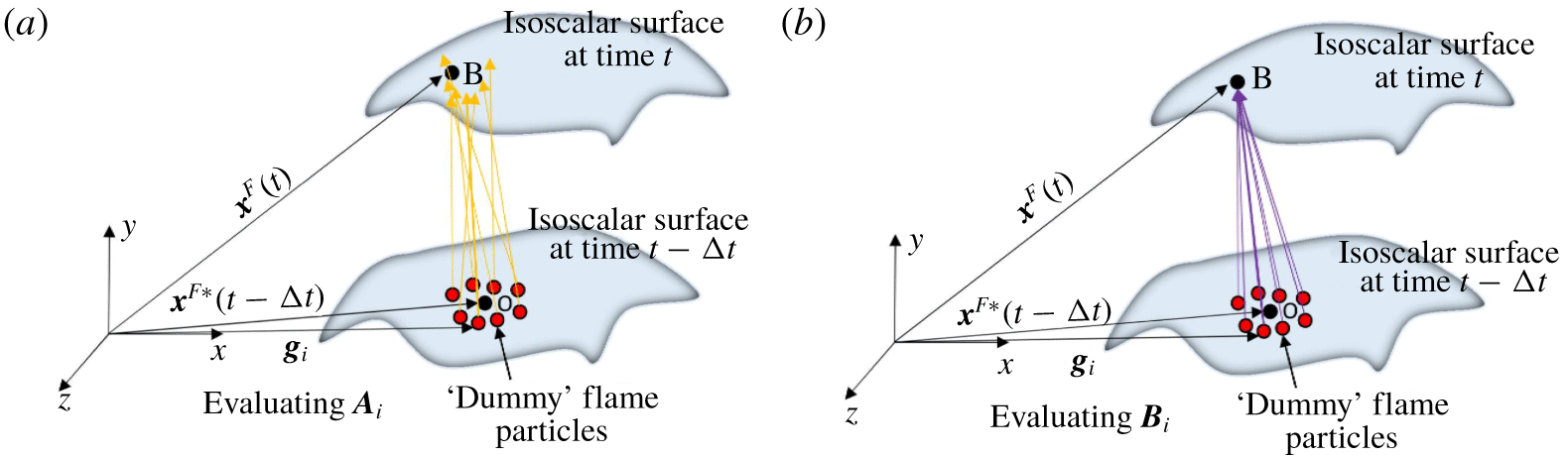
A schematic showing the correlation stage of the BFPT algorithm. In (a) the ‘available’ velocity  $\boldsymbol{A}_{i}$ is computed by interpolating
 $\boldsymbol{v}^{F}(t-\unicode[STIX]{x0394}t)$ at dummy flame particles. In (b) the ‘required’ velocity is computed as
 $\boldsymbol{B}_{i}=(\boldsymbol{x}^{F}(t)-\boldsymbol{g}_{i})/\unicode[STIX]{x0394}t$.

While backtracking, the discretized form of (1.1) cannot be integrated even numerically because the position at time  $t-\unicode[STIX]{x0394}t$ is unknown, and hence other parameters cannot be interpolated. Equation (2.1) shows this issue using a first-order accurate discretization scheme. The actual implementation of BFPT is second-order accurate.
 $$\begin{eqnarray}\boldsymbol{x}^{F}(t-\unicode[STIX]{x0394}t)=\boldsymbol{x}^{F}(t)+(-\boldsymbol{v}^{F}(t-\unicode[STIX]{x0394}t))\unicode[STIX]{x0394}t.\end{eqnarray}$$
To resolve this issue, the BFPT algorithm is implemented in two stages: estimation and correlation. During the estimation stage, as shown schematically in figure 2, we obtain an estimate for the flame particle position  $\boldsymbol{x}^{F\ast }$ at time
 $t-\unicode[STIX]{x0394}t$ (point O) by approximating
 $\boldsymbol{v}^{F}(t-\unicode[STIX]{x0394}t)$ as
 $\boldsymbol{v}^{F}(t)$ in (2.1). In the correlation stage our objective is to refine the estimate of point O. Therefore, first (see figure 3a), we define a large number (
 $i=1$ to
 $N$) of dummy flame particles with position vectors
 $\boldsymbol{g}_{i}$ in the local neighbourhood of
 $\boldsymbol{x}^{F\ast }$. Then, we interpolate
 $\boldsymbol{v}^{F}(t-\unicode[STIX]{x0394}t)$ from the Eulerian grid at all these points.
 $\boldsymbol{A}_{i}$ represents the available velocity vector at the
 $i$th dummy flame particle obtained on interpolation. Then, the required velocity vector
 $\boldsymbol{B}_{i}$ is obtained as
 $\boldsymbol{B}_{i}=(\boldsymbol{x}^{F}(t)-\boldsymbol{g}_{i})/\unicode[STIX]{x0394}t$, as shown schematically in figure 3(b). Finally, the correlation coefficient
 $D_{i}=\boldsymbol{A}_{i}\boldsymbol{\cdot }\boldsymbol{B}_{i}/\max \{|\boldsymbol{A}_{i}|,|\boldsymbol{B}_{i}|\}^{2}$ is calculated, such that
 $D\in [-1,1]$. The dummy flame particle which gives value of
 $D_{i}$ closest to 1 is chosen to be
 $\boldsymbol{x}^{F}(t-\unicode[STIX]{x0394}t)$. The above-mentioned steps are repeated for all other flame particles and at all subsequent time steps.
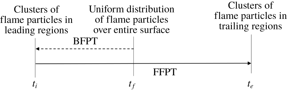
Schematic showing the relevance of different time instants  $t_{i}$,
 $t_{f}$ and
 $t_{e}$, and how the BFPT and FFPT simulations are performed in this study. All time instants (
 $t_{i}$,
 $t_{f}$ and
 $t_{e}$) relate to the statistically stationary state of the flame.

Figure 4 shows a schematic of the tracking simulations. In this study, we start tracking at time  $t_{f}$ using a uniform distribution of 2000 flame particles on isotherms. We arbitrarily chose the time instant
 $t_{f}$ to initialize the flame particles. Following the initialization, we first use BFPT to track the flame particles backward in time to some time instant
 $t_{i}$ and identify the generation locations i.e. the leading regions of the flame. Subsequently, we use the final state of flame particles from BFPT as the initial condition for FFPT and track the flame particles from time
 $t_{i}$ to some time
 $t_{e}$, such that
 $t_{i}<t_{f}<t_{e}$. By time
 $t_{e}$, a majority of the flame particles annihilate, and the remaining few occupy a negligible area, mostly in the negatively curved trailing regions of the flame. Thus, for the majority of the flame particles, BFPT followed by FFPT enables tracking of flame particles over their entire lifetimes. Hence, any arbitrary realization from the flame at any time must belong to some flame particles (not necessarily among the 2000 particles tracked) which are in between their generation and annihilation times. Tracking a large number of flame particles from generation to annihilation thus creates a manifold of states and statistics that can well describe any arbitrary flame dynamics belonging to the statistically stationary realization it corresponds to. Thus, while tracking it must be ensured that
 $t_{i},t_{f}$, and
 $t_{e}$ correspond to a statistically stationary condition of the flame.
3 Results and discussion
We have presented the results and the accompanying discussions in four main subsections. First, the general observations on the time evolution of specific properties at the flame particle locations from time  $t_{i}$ to
 $t_{e}$ are discussed.
3.1 General observations
In this study, we have used the flame particle tracking methodologies to track flame particles defined on three different isotherms:  $T_{0}=350~\text{K}$, 665 K and 1321 K, from each case;
 $T_{0}=350~\text{K}$ is close to the fresh reactants. Following the arguments used by Uranakara et al. (Reference Uranakara, Chaudhuri, Dave, Arias and Im2016), we have used
 $T_{0}=665~\text{K}$ and 1321 K as the other isotherms to represent the flame;
 $T_{0}=665~\text{K}$ and
 $T_{0}=1321~\text{K}$ are representative of the peak rates of the termination (
 $\text{H}+\text{O}_{2}+\text{M}=\text{HO}_{2}+\text{M}$) and branching (
 $\text{H}+\text{O}_{2}=\text{OH}+\text{O}$) reactions, respectively, for a standard premixed flame of an
 $\text{H}_{2}$–air mixture.
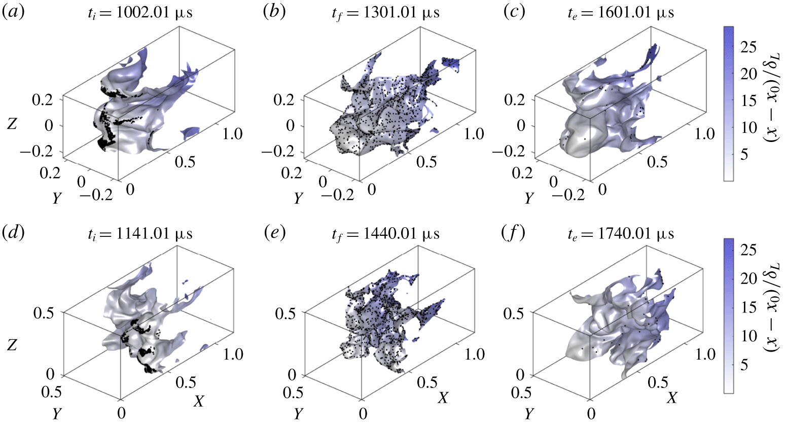
Figure 5 shows three instantaneous states of the isotherms along with the flame particles on it represented with the help of black dots. The results are qualitatively similar for the remaining isotherms and therefore not presented here. In each panel, fresh reactants enter the cuboid from the left plane and burned products leave from the right plane. Figures 5(a) and 5(d) show that, at time  $t_{i}$, where the BFPT ends and the FFPT begins, the flame particles are clustered in the leading regions of the flame surfaces. These regions are spatially most advanced, or ‘leading’, towards the fresh reactants. Figures 5(b) and 5(e) show that, at time
 $t_{f}$, the flame particles are spread over the entire flame surface. In other words, forward tracking of flame particles from leading regions over time
 $t_{i}$ to
 $t_{f}$ nearly recreates the initial condition of the BFPT simulation (refer to figure 4). By the time
 $t_{e}$ (shown in figures 5c and 5f), most flame particles have been annihilated and only a fraction of the initial number of flame particles survive. In summary, each panel in figure 5 shows that, as time progresses, new flame surface elements are generated from the leading regions which are predominantly positively curved, then, these flame surface elements stretch to form a complete flame surface at some intermediate time, and ultimately annihilate in the negatively curved regions near the trailing end of the flame surface. Amato & Lieuwen (Reference Amato and Lieuwen2014) have presented a theoretical study on the significance of leading points in an inhomogeneous laminar flow. By solving the conservation equation of the flame slope backward in time, they generated backward characteristic curves and identified conditions under which the large-time behaviour of the flame may or may not be controlled by discrete ‘leading’ points. However, for the DNS cases at moderate
 $Ka$ presented in this study, we observe that the leading points do play a significant role in generating surfaces at a later time. Dave et al. (Reference Dave, Abinesh and Chaudhuri2018) performed BFPT and discussed the time evolution of flame particles only for the duration from
 $t_{i}$ to
 $t_{f}$. Chaudhuri (Reference Chaudhuri2015) and Uranakara et al. (Reference Uranakara, Chaudhuri, Dave, Arias and Im2016) used FFPT on a uniform distribution of flame particles and tracked them to their annihilation. Their studies correspond to tracking of flame particles over the duration
 $t_{f}$ to
 $t_{e}$. Therefore, this study reports, for the first time, a description of the entire lifetime of flame particles – from generation to annihilation.
Instantaneous states of isotherm (or flame surface) corresponding to  $T_{0}=350~\text{K}$ from Case-L (a–c) and
 $T_{0}=665~\text{K}$ from Case-H (d–f) along with the flame particles, represented with the help of black dots. Flame surfaces are coloured with the normalized distance
 $(x-x_{0})/\unicode[STIX]{x1D6FF}_{L}$, where
 $x$ is the
 $X$-coordinate of points on the surface and
 $x_{0}=\text{min}(x)$.

During evolution, different flame particles annihilate at different instants of time  $t$. Therefore, examining the probability density functions (p.d.f.) in dimensional time
 $t$ would not be meaningful to obtain the flame particle annihilation statistics. Following Chaudhuri (Reference Chaudhuri2015) and Uranakara et al. (Reference Uranakara, Chaudhuri, Dave, Arias and Im2016), we define a normalized time coordinate
 $t/\unicode[STIX]{x1D70F}_{F,L}=(t-t_{i})/(t_{d}-t_{i})$, where
 $t_{i}$ corresponds to the initial condition of flame particles, and
 $t_{d}$ denotes the dimensional time when a given flame particle annihilates. Thus,
 $t_{d}\leqslant t_{e}$ and
 $t/\unicode[STIX]{x1D70F}_{F,L}\in [0,1]$. A small fraction of flame particles do survive until the end
 $t_{e}$ of the tracking simulation. However, such flame particles are not considered for further analysis and only those flame particles which annihilate are identified using the definition of
 $t/\unicode[STIX]{x1D70F}_{F,L}$. Therefore,
 $t/\unicode[STIX]{x1D70F}_{F,L}=0$ corresponds to the initial condition of flame particles and
 $t/\unicode[STIX]{x1D70F}_{F,L}=1$ corresponds to the time when they annihilate.
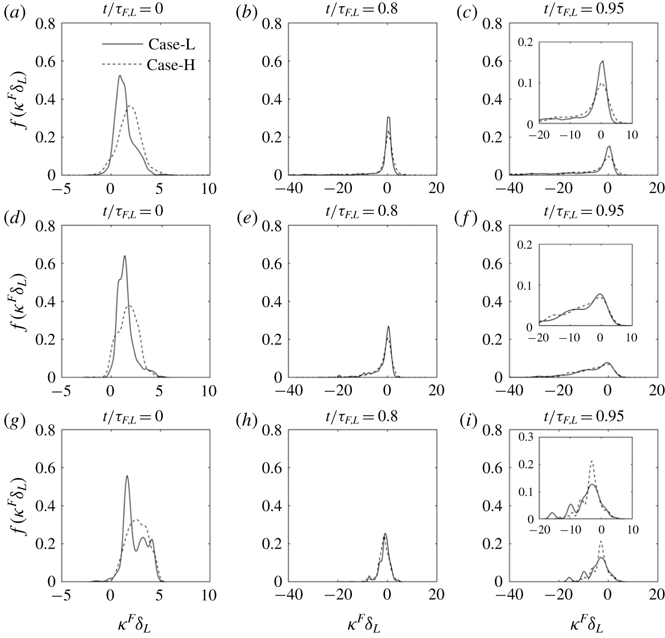
Probability density functions of normalized curvature  $\unicode[STIX]{x1D705}^{F}\unicode[STIX]{x1D6FF}_{L}$ evaluated at the flame particle locations at three different instants of normalized time
 $t/\unicode[STIX]{x1D70F}_{F,L}$ for both Case-L and Case-H. Panels (a–c) relate to the
 $T_{0}=350~\text{K}$ isotherm, (d–f) relate to the
 $T_{0}=665~\text{K}$ isotherm and (g–i) relate to the
 $T_{0}=1321~\text{K}$ isotherm. The insets in panels (c), (f) and (i) show a zoomed view of the corresponding p.d.f.

Figure 6 shows the p.d.f. of normalized curvature  $\unicode[STIX]{x1D705}^{F}\unicode[STIX]{x1D6FF}_{L}$ conditioned at the flame particles on the three isotherms at three different instants of
 $t/\unicode[STIX]{x1D70F}_{F,L}$, for both Case-L and Case-H. The first, second and third rows relate to
 $T_{0}=350~\text{K}$, 665 K and 1321 K, respectively. Figures 6(a), 6(d) and 6(g) show that, at the initial time (
 $t/\unicode[STIX]{x1D70F}_{F,L}=0$), the leading regions occupied by the flame particles are positively curved. From figures 6(b), 6(e) and 6(h), plotted at
 $t/\unicode[STIX]{x1D70F}_{F,L}=0.8$, one can observe that the p.d.f. of
 $\unicode[STIX]{x1D705}^{F}\unicode[STIX]{x1D6FF}_{L}$ shows a significant negative tail and the local geometry of the majority of flame particles is such that they have zero curvature. Therefore, consistent with the observations from figure 5, we can say that, as time progress, flame particles disperse from the positively curved leading regions and begin to occupy regions of both positive and negative curvature. Figures 6(c), 6(f) and 6(i) show that the negative tail of the p.d.f. develops further. This demonstrates that, further in time, flame particles travel to regions of larger negative curvature and eventually annihilate.
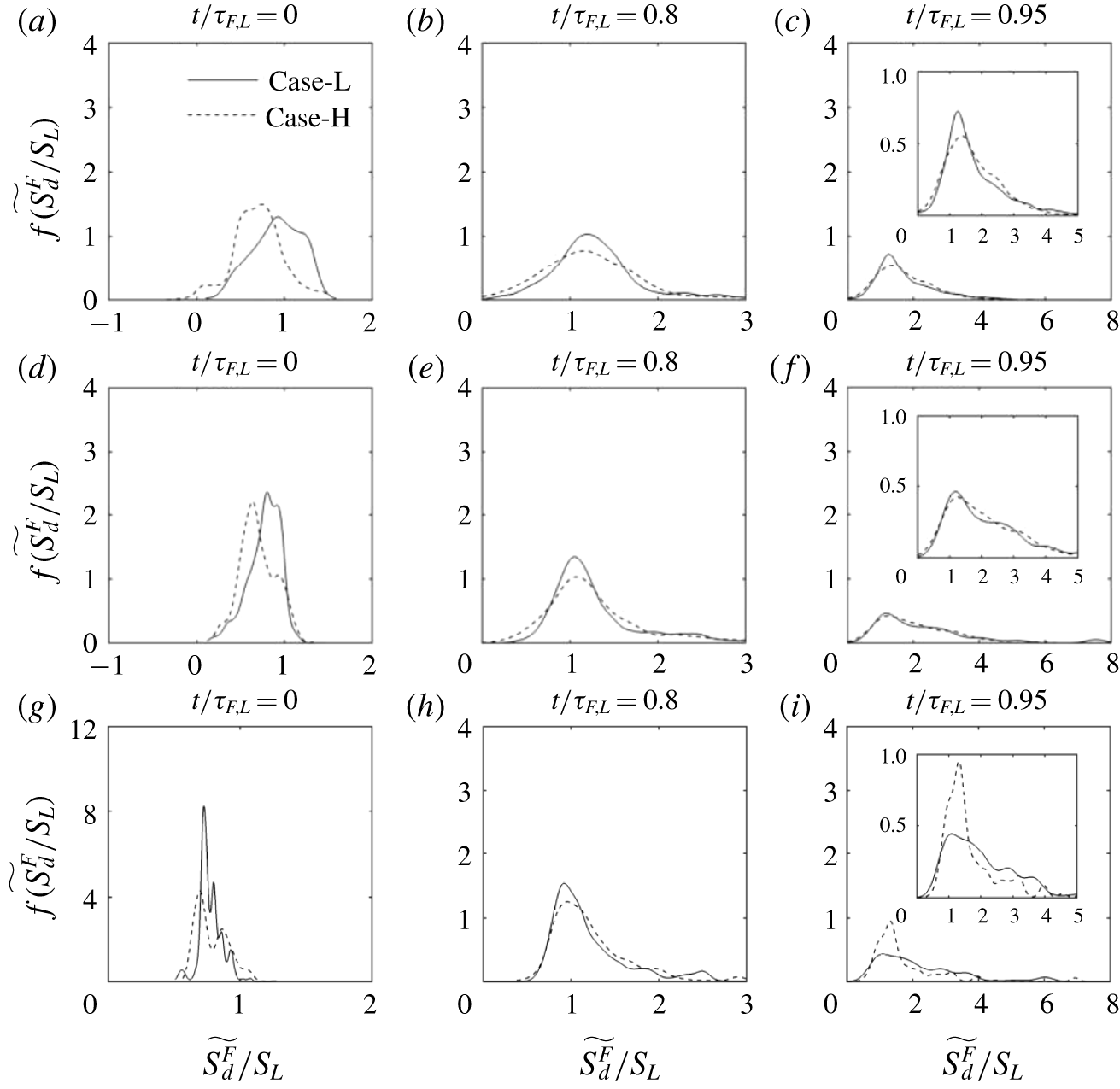
Probability density functions of normalized density-weighted flame displacement speed  $\widetilde{S_{d}^{F}}/S_{L}$ evaluated at the flame particle locations at three different instants of normalized time
 $t/\unicode[STIX]{x1D70F}_{F,L}$ for both Case-L and Case-H. Panels (a–c) relate to the
 $T_{0}=350~\text{K}$ isotherm, (d–f) relate to the
 $T_{0}=665~\text{K}$ isotherm and (g–i) relate to the
 $T_{0}=1321~\text{K}$ isotherm. The insets in panels (c), (f) and (i) show a zoomed view of the corresponding p.d.f.

Figure 7 shows the p.d.f. of  $\widetilde{S_{d}^{F}}$ normalized by
 $S_{L}$ evaluated at the flame particle locations. Again, the first, second and third rows relate to
 $T_{0}=350~\text{K}$, 665 K and 1321 K, respectively. Figures 7(a), 7(d) and 7(g) clearly show that the flame particles start propagating from the leading regions with
 $\widetilde{S_{d}^{F}}\sim O(S_{L})$. Since the regions of the flame surface occupied by the flame particles initially are positively curved and may experience strain due to the underlying turbulent flow field, it can be expected that the distribution of
 $\widetilde{S_{d}^{F}}$ around
 $S_{L}$ is a manifestation of the flame response to the stretch and curvature effects. Figures 7(b), 7(e) and 7(h) show that, as time progresses, the p.d.f. of the local propagation speed
 $\widetilde{S_{d}^{F}}$ becomes wide and many regions propagate with
 $\widetilde{S_{d}}$ greater than
 $S_{L}$. Since these panels correspond to
 $t/\unicode[STIX]{x1D70F}_{F,L}=0.8$, they also indicate that, for a significant part of the lifetime of flame particles, the propagation characteristics vary in the vicinity of
 $S_{L}$. Figures 7(c), 7(f) and 7(i), however, show that, towards the end of the flame particle lifetime, in the negatively curved regions, a large number of flame particles experience a steep rise in the flame displacement speed, and
 $\widetilde{S_{d}^{F}}$ becomes significantly larger than
 $S_{L}$ over a rather short duration of time. These large excursions of
 $\widetilde{S_{d}}$ away from
 $S_{L}$ need to be understood. Despite the important insights from the studies of Echekki, Chen & Gran (Reference Echekki, Chen and Gran1996) and Chen, Echekki & Kollmann (Reference Chen, Echekki and Kollmann1999), a systematically derived model for the flame displacement speed during the annihilation of flame elements has not been reported in the literature yet.
3.2 Phase-I: non-interacting phase
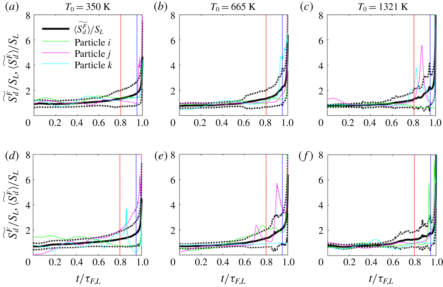
Comparison of the time evolution of normalized density-weighted flame displacement speed  $\widetilde{S_{d}^{F}}/S_{L}$ for three flame particles with the ensemble average.
 $\langle \;\rangle$ denotes ensemble averaging over all the flame particles at a given instant of
 $t/\unicode[STIX]{x1D70F}_{F,L}$. Panels (a–c) relate to Case-L and (d–f) relate to Case-H. The ensemble average is represented with a solid black line. The black dotted lines around it represents
 $(\pm )$ one standard deviation from the ensemble average. The vertical red line at
 $t/\unicode[STIX]{x1D70F}_{F,L}=0.8$ separates the two phases in the lifetime of a flame particle. The p.d.f. at
 $t/\unicode[STIX]{x1D70F}_{F,L}=0.95$ corresponding to the blue line is shown in the last column of figure 7.

Figure 8 shows the time evolution of the normalized density-weighted flame displacement speed  $\widetilde{S_{d}^{F}}/S_{L}$ for three arbitrarily chosen flame particles and compares them with the ensemble average
 $\langle \widetilde{S_{d}^{F}}\rangle /S_{L}$ and one standard deviation from the ensemble average, evaluated over all the flame particles at a given instant of
 $t/\unicode[STIX]{x1D70F}_{F,L}$. While figure 7 presented the p.d.f. at discrete values of
 $t/\unicode[STIX]{x1D70F}_{F,L}$, figure 8 shows the continuous time evolution of the ensemble average and also one standard deviation from it. Figures 8(a), 8(b) and 8(c) correspond to the
 $T_{0}=350~\text{K}$, 665 K and 1321 K isotherms from Case-L, respectively. The second row shows figures for the same isotherms from Case-H. Each panel clearly shows that
 $\widetilde{S_{d}^{F}}$ of the three flame particles remains close to
 $S_{L}$ for a significant part of the flame particle’s lifetime (nearly 80 %). Few flame particles can show large deviations of
 $\widetilde{S_{d}^{F}}$ from
 $S_{L}$ even for
 $t/\unicode[STIX]{x1D70F}_{F,L}<0.8$, and such occurrences are very rare. The relatively smooth and gradual variation of
 $\langle \widetilde{S_{d}^{F}}\rangle /S_{L}$, represented using a thick solid line, corroborates this conjecture. Thus, we can infer from figures 7 and 8 that we can define a duration up to
 $t/\unicode[STIX]{x1D70F}_{F,L}=0.8$, which is identified in figure 8 with the help of a solid vertical red line, up to which
 $\widetilde{S_{d}^{F}}$ varies slowly in the vicinity of
 $S_{L}$ for the majority of flame particles and consequently for their ensemble average. In other words, over this duration (
 $0\leqslant t/\unicode[STIX]{x1D70F}_{F,L}\leqslant 0.8$) which we refer to as Phase-I,
 $\widetilde{S_{d}^{F}}/S_{L}$ is not too far from 1. Flame particles experience a steep rise in the flame displacement speed and
 $\widetilde{S_{d}^{F}}$ deviates significantly away from
 $S_{L}$ over the remaining small fraction of their lifetime
 $0.8<t/\unicode[STIX]{x1D70F}_{F,L}\leqslant 1$, referred to as Phase-II.
Now, we assess the applicability of the two-parameter Markstein length model (1.6) at the flame particle locations. Phenomenologically, the Markstein length theory, which is valid in the weak-stretch limit, can, at best, capture the deviations in  $\widetilde{S_{d}^{F}}$ in the vicinity of
 $S_{L}$. Hence, the performance of (1.6) may deteriorate significantly as the flame particles progress towards annihilation. Therefore, it seems logical that we assess the applicability of (1.6) separately over the two phases. In the second phase, if the error in prediction using (1.6) is unacceptable, we have to investigate the possible reasons and either modify the existing model or look for a new one if modification is not a viable option. Later, we will show that the latter case prevails and we, therefore, propose a new model for the second phase. In this subsection, our emphasis is on Phase-I.
In (1.6), stretch rate  $K=(1/\unicode[STIX]{x1D6FF}A)\,\text{d}(\unicode[STIX]{x1D6FF}A)/\text{d}t$ is an important input parameter and it measures the fractional rate of change in area for an infinitesimal area element
 $\unicode[STIX]{x1D6FF}A$ on a flame surface. Matalon (Reference Matalon1983), Chung & Law (Reference Chung and Law1984) and Candel & Poinsot (Reference Candel and Poinsot1990) have derived expressions for
 $K$. Equation (3.1) shows how
 $K$ is related to tangential strain rate
 $a_{T}$ and the curvature-propagation term
 $S_{d}\unicode[STIX]{x1D705}$:
 $$\begin{eqnarray}K=\underbrace{\unicode[STIX]{x1D735}\boldsymbol{\cdot }\boldsymbol{u}-\boldsymbol{n}\boldsymbol{n}\boldsymbol{ : }\unicode[STIX]{x1D735}\boldsymbol{u}}_{a_{T}}+S_{d}\unicode[STIX]{x1D705}.\end{eqnarray}$$
When the general expression (3.1) for  $K$ is evaluated at the flame particle locations and used in (1.6), we get an expression for
 $\widetilde{S_{d}^{F}}/S_{L}$ as follows:
 $$\begin{eqnarray}\frac{\widetilde{S_{d}^{F}}}{S_{L}}=\frac{1-{\mathcal{L}}_{K}a_{T}^{F}/S_{L}-{\mathcal{L}}_{\unicode[STIX]{x1D705}}\unicode[STIX]{x1D705}^{F}}{1+\unicode[STIX]{x1D703}^{\ast }{\mathcal{L}}_{K}\unicode[STIX]{x1D705}^{F}}.\end{eqnarray}$$
Since for subsonic flames  $\unicode[STIX]{x1D70C}\sim 1/T$,
 $\unicode[STIX]{x1D70C}_{u}/\unicode[STIX]{x1D70C}_{0}\approx T_{0}/T_{u}$ and
 $\unicode[STIX]{x1D703}^{\ast }=T_{0}/T_{u}$ is the non-dimensional temperature, as noted earlier. It can be seen that (3.2) is relatively complex where the denominator can lead to unreasonable predictions as
 $\unicode[STIX]{x1D703}^{\ast }{\mathcal{L}}_{K}\unicode[STIX]{x1D705}^{F}$ tends to
 $-1$. These issues can be addressed by defining appropriate models for the stretch rate. In the hydrodynamic limit, where the flame collapses to a flame sheet, (3.3) is used to model
 $K$. The effect of dilatation
 $\unicode[STIX]{x1D735}\boldsymbol{\cdot }\boldsymbol{u}$ is not accounted for and
 $S_{d}$ is approximated with
 $S_{L}$ in the curvature-propagation term (see Matalon et al. Reference Matalon, Cui and Bechtold2003). It can be seen that
 $K^{\ast }$ will model
 $K$ appropriately if the selected isotherms are closer to the fresh reactants.
 $$\begin{eqnarray}K^{\ast }=\underbrace{-\boldsymbol{n}\boldsymbol{n}\boldsymbol{ : }\unicode[STIX]{x1D735}\boldsymbol{u}}_{K_{s}}+S_{L}\unicode[STIX]{x1D705}.\end{eqnarray}$$
When we use  $K^{\ast }$ to approximate the stretch rate at the flame particle locations, (1.6) can be rewritten as follows:
 $$\begin{eqnarray}\frac{\widetilde{S_{d}^{F}}}{S_{L}}=1-\frac{{\mathcal{L}}_{K}K^{\ast F}}{S_{L}}-{\mathcal{L}}_{\unicode[STIX]{x1D705}}\unicode[STIX]{x1D705}^{F}.\end{eqnarray}$$
Since in this study we define isotherms within a flame, it can be anticipated that  $K^{\ast }$ may not be suitable and another model may be required to model stretch rate. Figures 7 and 8 shows that, over Phase-I, the variations in
 $\widetilde{S_{d}}$ are closer to
 $S_{L}$. Therefore, for the curvature-propagation term in
 $K$, we have used
 $S_{d}\approx S_{L}\unicode[STIX]{x1D70C}_{u}/\unicode[STIX]{x1D70C}_{0}\approx S_{L}\unicode[STIX]{x1D703}^{\ast }$, where
 $\unicode[STIX]{x1D703}^{\ast }=T_{0}/T_{u}$. The new model for
 $K$ is
 $K^{\prime }$ and is given by (3.5). It should be noted that
 $K^{\prime }$ is suitable only over Phase-I because
 $S_{d}\approx S_{L}\unicode[STIX]{x1D703}^{\ast }$ is not a good approximation over Phase-II where the flame particles experience steep acceleration and
 $\widetilde{S_{d}}$ is significantly larger than
 $S_{L}$.
 $$\begin{eqnarray}K^{\prime }=\unicode[STIX]{x1D735}\boldsymbol{\cdot }\boldsymbol{u}-\boldsymbol{n}\boldsymbol{n}:\unicode[STIX]{x1D735}\boldsymbol{u}+S_{L}\unicode[STIX]{x1D703}^{\ast }\unicode[STIX]{x1D705}.\end{eqnarray}$$
When we use  $K^{\prime }$ to evaluate the stretch rate at the flame particle locations, (1.6) can be rewritten as follows:
 $$\begin{eqnarray}\frac{\widetilde{S_{d}^{F}}}{S_{L}}=1-\frac{{\mathcal{L}}_{K}}{S_{L}}a_{T}^{F}-({\mathcal{L}}_{K}\unicode[STIX]{x1D703}^{\ast }+{\mathcal{L}}_{\unicode[STIX]{x1D705}})\unicode[STIX]{x1D705}^{F}.\end{eqnarray}$$
It is to be recognized that (1.6) or its modified form (3.4) are obtained from rigorous asymptotic analysis, where  ${\mathcal{L}}_{K}$ and
 ${\mathcal{L}}_{\unicode[STIX]{x1D705}}$ are of
 $O(\ell _{f})$ and
 $\ell _{f}\ll L$, and other quantities are of
 $O(1)$. Thus (3.4) is accurate up to
 $O(\ell _{f})$. While deriving (3.2) and (3.6), the effect of dilatation is included. Moreover, the curvature contribution to stretch rate is either taken completely or modelled. These modifications may include some
 $O(\ell _{f}^{2})$ terms in (3.2) and (3.6) but not all
 $O(\ell _{f}^{2})$ contributions. While it will be shown later that (3.6) performs best in predicting the DNS results, it is not necessarily consistent with the asymptotic results and neither is (3.2). However, (3.6) can be treated as a necessary practical modification to apply the asymptotic solution within flames of finite thickness and non-zero dilatation. The only fully consistent asymptotic result is given by (3.4). In any case, all these equations will be compared with the DNS results in the following.
To calculate the Markstein lengths  ${\mathcal{L}}_{K}$ and
 ${\mathcal{L}}_{\unicode[STIX]{x1D705}}$, we have used the following parameters from the work of Sun et al. (Reference Sun, Sung, He and Law1999). The limiting Lewis number
 $Le_{F}=0.33$ and
 $Le_{O}=2.32$ in the lean and rich flammability limits, respectively. Overall activation energy
 $E_{a}=28.7~\text{kcal}~\text{mol}^{-1}$. Other parameters, such as
 $T_{b}=2176~\text{K}$, the exponent for variation of transport properties
 $a=0.61$,
 $\unicode[STIX]{x1D6FC}_{u}=0.454$cm
 $^{2}$/s, etc. were obtained from the solution of the standard premixed flame using the PREMIX (Kee et al. Reference Kee, Grcar, Smooke, Miller and Meeks1985) code. Using the above values we find a Zeldovich number of
 $\unicode[STIX]{x1D6FD}=5.7$ and
 $Le_{eff}=0.93$ for the
 $\text{H}_{2}$–air mixture with
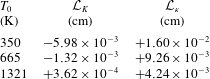
 $\unicode[STIX]{x1D719}=0.81$ used in this study. Table 2 shows the values of
 ${\mathcal{L}}_{K}$ and
 ${\mathcal{L}}_{\unicode[STIX]{x1D705}}$ for
 $T_{0}=350~\text{K}$, 665 K and 1321 K. It also shows that
 ${\mathcal{L}}_{K}$ varies from negative to a small positive number as we move from
 $T_{0}=350~\text{K}$ to
 $T_{0}=1321~\text{K}$ across the thickness of the flame, while simultaneously we observe a monotonic drop in
 ${\mathcal{L}}_{\unicode[STIX]{x1D705}}$. These values are qualitatively consistent with the observations reported by Giannakopoulos et al. (Reference Giannakopoulos, Gatzoulis, Frouzakis, Matalon and Tomboulides2015). Next we assess how (3.2), (3.4) and (3.6) perform to predict the local
 $\widetilde{S_{d}^{F}}$ along the trajectories of flame particles and compare them with the values at the flame particles obtained directly from the DNS.
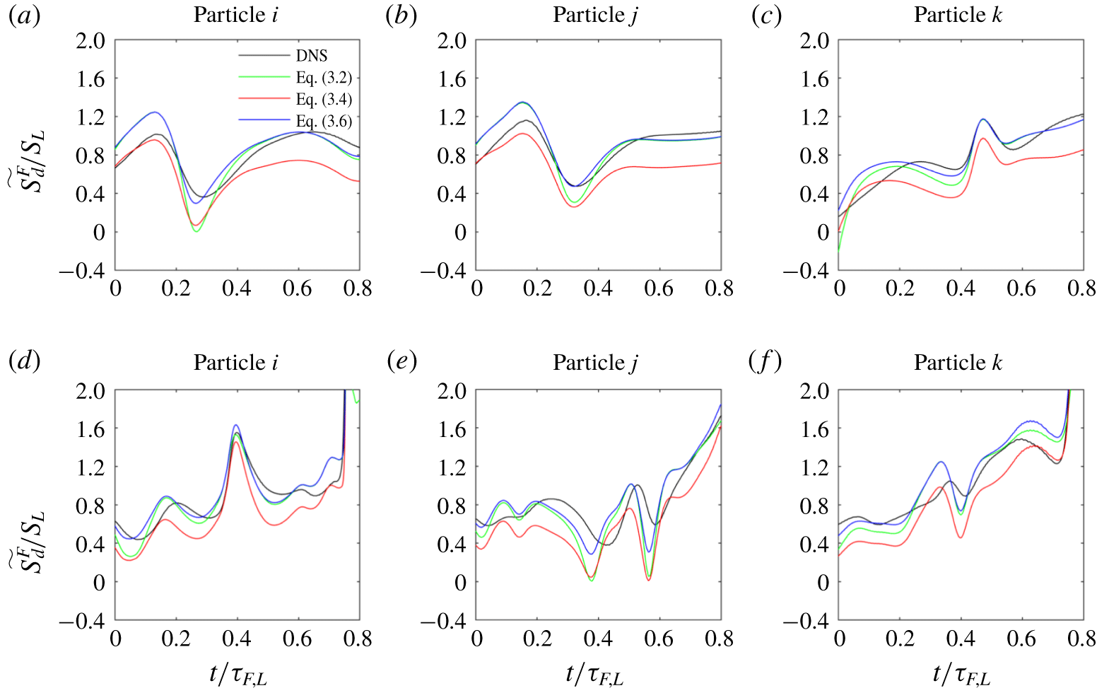
Comparison of  $\widetilde{S_{d}^{F}}/S_{L}$ between DNS and model ((3.2), (3.4) and (3.6)) over Phase-I (
 $t/\unicode[STIX]{x1D70F}_{F,L}\leqslant 0.8$) of three flame particles. Panels (a–c) in the first row relate to flame particles from Case-L and panels (d–f) in the second row relate to flame particles on
 $T_{0}=665~\text{K}$ isotherm from Case-H.

Stretch and curvature Markstein lengths for the  $\text{H}_{2}$–air mixture used in this study. Using the global reaction parameters presented by Sun et al. (Reference Sun, Sung, He and Law1999), we obtain
 $Le_{F}=0.33$,
 $Le_{O}=2.32$ and
 $E_{a}=28.7~\text{kcal}~\text{mol}^{-1}$. While calculating
 $Le_{eff}=0.93$, the reaction orders with respect to fuel and oxidiser were assumed to be 1. For
 $\unicode[STIX]{x1D719}=0.81$,
 $P=1~\text{atm}$ and
 $T_{u}=310~\text{K}$, the parameters
 $T_{b}=2176~\text{K}$,
 $S_{L}=185~\text{cm}~\text{s}^{-1}$,
 $\unicode[STIX]{x1D6FC}_{u}=0.454~\text{cm}^{2}~\text{s}^{-1}$ and temperature exponent
 $a=0.61$ were calculated from the output of the PREMIX code. All these values were then used to calculate
 ${\mathcal{L}}_{K}$ and
 ${\mathcal{L}}_{\unicode[STIX]{x1D705}}$ above.

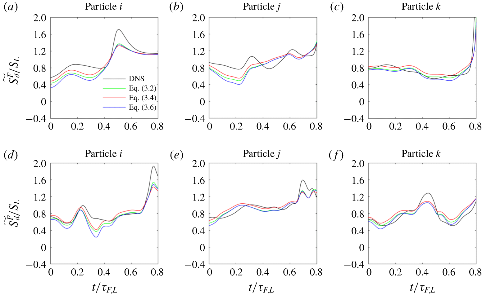
Comparison of  $\widetilde{S_{d}^{F}}/S_{L}$ between DNS and model ((3.2), (3.4) and (3.6)) over Phase-I (
 $t/\unicode[STIX]{x1D70F}_{F,L}\leqslant 0.8$) of three flame particles. Panels (a–c) in the first row relate to flame particles on
 $T_{0}=1321~\text{K}$ isotherm from Case-L and panels (d–f) in the second row relate to flame particles on
 $T_{0}=1321~\text{K}$ isotherm from Case-H.

Figures 9 and 10 show the comparison of  $\widetilde{S_{d}^{F}}/S_{L}$ between the DNS and the two-parameter Markstein length model with different definitions of stretch rate at the flame particle locations for
 $T_{0}=665~\text{K}$ and 1321 K, respectively. The comparison is made along the trajectories of three representative flame particles over Phase-I. Figures 9(a)–9(c) relate to the flame particles on the
 $T_{0}=665~\text{K}$ isotherm from Case-L, while figures 9(d)–9(f) relate to the flame particles on
 $T_{0}=665~\text{K}$ isotherm from Case-H. Figure 10, belonging to
 $T_{0}=1321~\text{K}$, can be read in a similar way. We refer to the Phase-I as the non-interacting phase also, where non-interacting implies that the flame is not directly interacting with any of its other flame parts. The figures indicate that the two-parameter Markstein length model can capture the qualitative trends in the local
 $\widetilde{S_{d}^{F}}$ with reasonable accuracy over Phase-I. As noted earlier, the variations in
 $\widetilde{S_{d}^{F}}$ over this phase are mild and, to the leading order, close to
 $S_{L}$. It can also be noted that the difference among the predictions using the (3.2), (3.4) and (3.6) is relatively greater in figure 9 than figure 10. This is because
 ${\mathcal{L}}_{K}$ for the
 $T_{0}=1321~\text{K}$ isotherm is nearly an order of magnitude smaller than
 ${\mathcal{L}}_{K}$ for the
 $T_{0}=665~\text{K}$ isotherm (see table 2) and the predictions are, therefore, less sensitive to the differences in the evaluated stretch rate. Next, we will quantify these observations with the help of error plots and give a rationale for the selection of an appropriate definition of stretch rate. Nevertheless, figures 9 and 10 demonstrate the applicability of modelling theories based on Markstein lengths developed for steady laminar flames and give unprecedented support to the significance of the two distinct Markstein lengths,
 ${\mathcal{L}}_{K}$ and
 ${\mathcal{L}}_{\unicode[STIX]{x1D705}}$ (Bechtold & Matalon (Reference Bechtold and Matalon2001) and Giannakopoulos et al. (Reference Giannakopoulos, Gatzoulis, Frouzakis, Matalon and Tomboulides2015)), in predicting the flame displacement speed for turbulent premixed flames where the local flame structure can be perturbed by the turbulent flow field at a multitude of length scales and time scales.
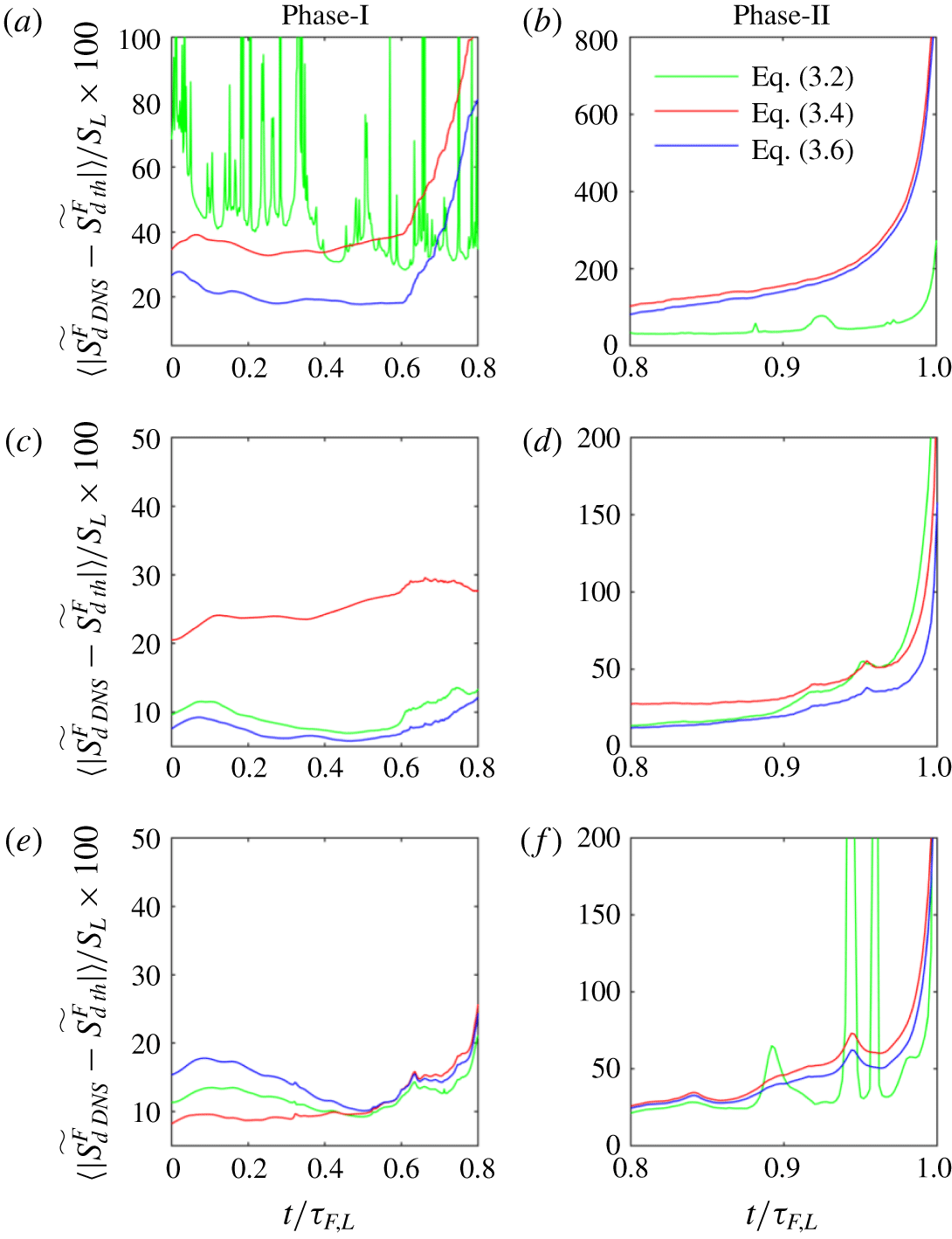
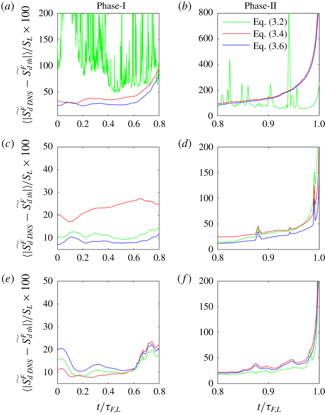
Comparison of relative error in prediction of flame displacement speed for the different definitions of stretch rate ((3.1), (3.3) and (3.5)) with respect to the results from DNS of Case-L. Panels (a,b), (c,d) and (e,f) correspond to  $T_{0}=350~\text{K}$, 665 K and 1321 K isotherms, respectively. Panels (a,c,e) correspond to Phase-I and (b,d,f) to Phase-II.

Comparison of relative error in prediction of flame displacement speed for the different definitions of stretch rate ((3.1), (3.3) and (3.5)) with respect to the results from DNS of Case-H. Panels (a,b), (c,d) and (e,f) correspond to  $T_{0}=350~\text{K}$, 665 K and 1321 K isotherms, respectively. Panels (a,c,e) correspond to Phase-I and (b,d,f) to Phase-II.

To assess which definition of stretch rate is more suitable for evaluating  $\widetilde{S_{d}^{F}}$ and also to quantify the accuracy of the two-parameter Markstein length model, we compare the errors for (3.2), (3.4) and (3.6). The relative error is computed as shown below:
 $$\begin{eqnarray}\unicode[STIX]{x1D716}(t/\unicode[STIX]{x1D70F}_{F,L})=\frac{\langle |(\widetilde{S_{d}^{F}}_{DNS}(t/\unicode[STIX]{x1D70F}_{F,L})-\widetilde{S_{d}^{F}}_{th}(t/\unicode[STIX]{x1D70F}_{F,L}))|\rangle }{S_{L}},\end{eqnarray}$$
where  $\widetilde{S_{d}^{F}}_{DNS}$ is obtained directly from the DNS while
 $\widetilde{S_{d}^{F}}_{th}$ is obtained from either (3.2), (3.4) or (3.6) at the flame particle locations. Figures 11 and 12 show the time series of the relative percentage error for Case-L and Case-H, respectively. First, figures 11(c), 11(e), 12(c) and 12(e) show that, irrespective of the turbulence Reynolds number, the performance of the Markstein length based theoretical model is reasonably accurate for Phase-I of the flame particle’s lifetime. The error in these panels for either definition is typically less than 30 %, which is acceptable even for extraction of
 $S_{L}$ from stretched laminar premixed flames (see Wu et al. (Reference Wu, Liang, Chen, Ju and Law2015) and Liang, Wu & Law (Reference Liang, Wu and Law2017)). Taking a cue from figure 6, these observations translate to the understanding that the regions of the flame surfaces which are not significantly negatively curved will observe a good agreement with the Markstein length theory. As will be discussed later, extremely curved regions on a flame surface with negative curvature are very prone to local flame–flame interactions, which completely change the local thermal and chemical structures. After the flame–flame interactions, the local flame elements usually experience annihilation, therefore, the stretch rate is also large and negative in such regions. Figures 11(d), 11(f), 12(d) and 12(f) show that the performance of the theoretical models quickly deteriorates over the remaining 20 % of the flame particle lifetime, i.e. Phase-II. In fact, the error rises sharply and blows up even beyond 200 %. Thus, the two-parameter Markstein length model gives unacceptable predictions for the second phase, irrespective of the definition of stretch rate. Finally, the first rows in both figures 11 and 12 corresponding to
 $T_{0}=350~\text{K}$ and also figure 11(f) highlight a crucial aspect of the feasibility of the general definition of stretch rate. In (3.2), a curvature term appears in the denominator. If
 $\unicode[STIX]{x1D703}^{\ast }{\mathcal{L}}_{K}\unicode[STIX]{x1D705}^{F}$ is negative and of
 $O(1)$, then the denominator of the right-hand side can get very close to zero. The near zero values of the denominator will lead to unreasonable predictions for the flame displacement speed. Since,
 ${\mathcal{L}}_{K}$ changes sign from negative to positive as the level-set temperature value increases, it can be easily seen that such instances may happen for
 $\unicode[STIX]{x1D705}^{F}>0$ (
 $\unicode[STIX]{x1D705}^{F}<0$) for isotherms with
 ${\mathcal{L}}_{K}<0$ (
 ${\mathcal{L}}_{K}>0$). While large negative curvature for local flame elements is common in turbulent premixed flames, Uranakara, Chaudhuri & Lakshmisha (Reference Uranakara, Chaudhuri and Lakshmisha2017) have shown that pointed positively curved flame surfaces can form during the extinction of ignition kernels in turbulence. Thus, the singularity in (3.2) is the reason behind the sudden large jumps in error for (3.2) in these panels. On the other hand, no such singularity appears in (3.4) and (3.6). The performance of (3.6) is better than (3.4) over Phase-I. However, still this does not spare any equation of the Markstein length based models from becoming unacceptable in Phase-II. Additionally, while (3.4) and (3.6) are amenable to term by term averaging, equation (3.2) is not. Therefore, figures 9–12 suggest that, first, using the Markstein length theory is fruitful only for portions where no flame–flame interactions occur, and second, although
 $K^{\prime }$ (3.5) is not consistent with asymptotic analysis it is nevertheless suitable to approximate the stretch rate in such non-interacting regions and can be subsequently used in the two-parameter Markstein length model.
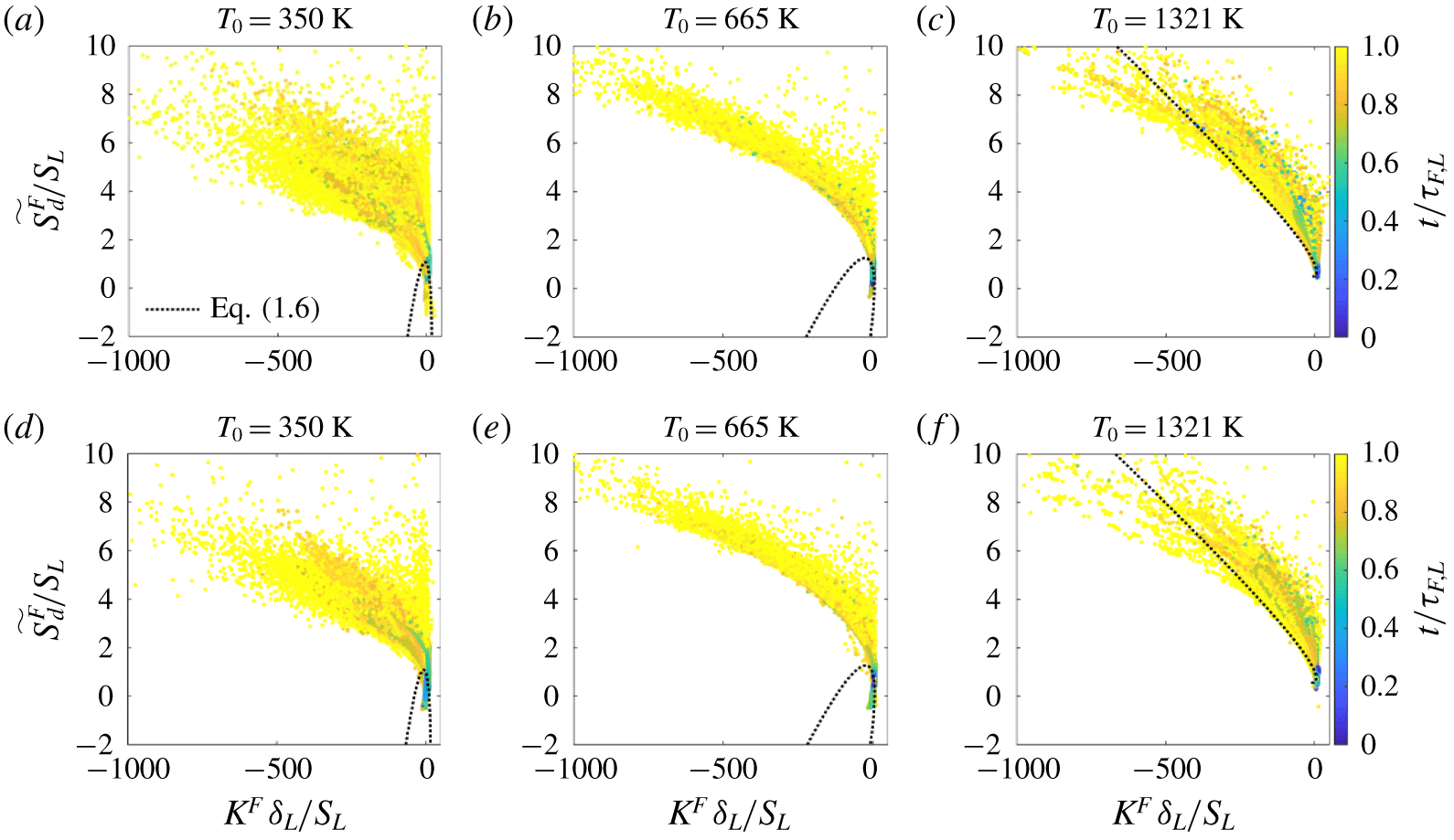
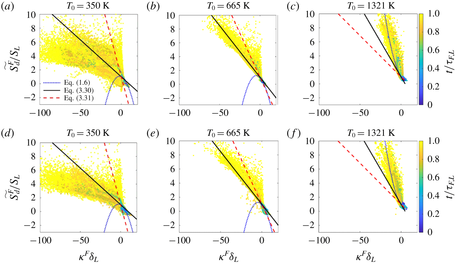
Time series of  $\widetilde{S_{d}^{F}}/S_{L}$ with respect to normalized stretch rate
 $K^{F}\unicode[STIX]{x1D6FF}_{L}/S_{L}$ evaluated at the flame particle locations. Panels (a–c) relate to Case-L and (d–f) relate to Case-H. The coloured dots represent the time-series data evaluated along the trajectories of all the flame particles and show the evolution of parameters in normalized time. The dotted block curve shows the prediction from (1.6).

Figure 13 shows a scatter of the time evolution of  $\widetilde{S_{d}^{F}}/S_{L}$ evaluated at the flame particle locations with respect to normalized stretch rate
 $K^{F}\unicode[STIX]{x1D6FF}_{L}/S_{L}$ over the entire duration, which includes both Phase-I and Phase-II. The colour bars depicting normalized time are shown at the right-hand side in each row and are common to the remaining panels in that row. For the sake of comparison, we have also shown the prediction from the model, i.e. (1.6). However, in these figures, the model is no longer compared along the trajectories of individual flame particles as when using (3.2), (3.4) and (3.6), but for the entire ensemble simultaneously, which requires knowledge of the variation of stretch rate and curvature for the ensemble. We have used a quadratic fit between the distribution of stretch rate
 $K^{F}$ with respect to curvature
 $\unicode[STIX]{x1D705}^{F}$. The entire range of values that these parameters take for the ensemble of flame particles is considered to obtain a fit. It must be noted that the variation of
 $K^{F}$ with respect to
 $\unicode[STIX]{x1D705}^{F}$ need not necessarily be a quadratic function, but the quadratic fit captures the trends reasonably well. Using the fit to generate stretch rate for a given value of curvature, one can then obtain a prediction of
 $\widetilde{S_{d}^{F}}/S_{L}$ using (1.6). Such a prediction of
 $\widetilde{S_{d}^{F}}/S_{L}$ with respect to
 $K^{F}\unicode[STIX]{x1D6FF}_{L}/S_{L}$ is plotted as a dotted black curve in figures 13(a)–13(f) for the ensemble of flame particles. In this study, figures 6(c), 6(f) and 6(i) already showed that
 $\unicode[STIX]{x1D705}^{F}\unicode[STIX]{x1D6FF}_{L}$ is large and negative towards the end of the lifetime of the flame particles. Each panel in figure 13 clearly shows that these regions also experience very large values of stretch rate. It may be anticipated that highly negatively curved flame elements with a radius of curvature of the order of the flame thickness, say
 $\unicode[STIX]{x1D6FF}_{L}$, can have a higher probability of flame–flame interactions. Usually, after such interactions the flame elements annihilate, consequently leading to large negative values of stretch rate. This may be the reason for a strong correlation between large negative curvature and large negative stretch rate which has also been discussed by Hawkes & Chen (Reference Hawkes and Chen2005). The value of
 $\widetilde{S_{d}^{F}}$ shows significant deviation from
 $S_{L}$ over Phase-II when flame particles are predominantly located in such regions. Figures 13(a,b) and 13(d,e), corresponding to
 $T_{0}=350~\text{K}$ and 665 K, show that the trend of
 $\widetilde{S_{d}^{F}}/S_{L}$ predicted by the model for the large stretch-rate regime is opposite to what one observes from the DNS data at the flame particles. This is also the reason behind the large error (even greater than 100 %) observed over Phase-II in figures 11 and 12. Except for
 $T_{0}=1321~\text{K}$ (figures 13c and 13f) for which the stretch Markstein length
 ${\mathcal{L}}_{K}$ is very low, the performance of (1.6) quickly deteriorates and cannot capture the large excursions of
 $\widetilde{S_{d}}$ away from
 $S_{L}$. Hence, the observation for the dramatic increase in the error for
 $t/\unicode[STIX]{x1D70F}_{F,L}>0.8$ as shown in figures 11 and 12 stands consistent.
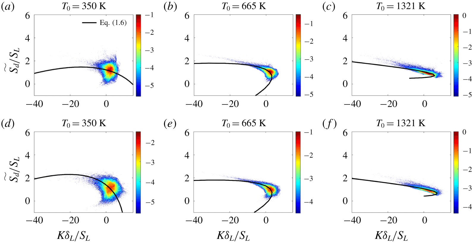
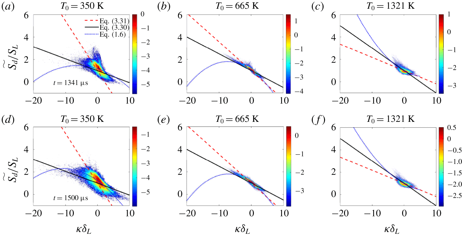
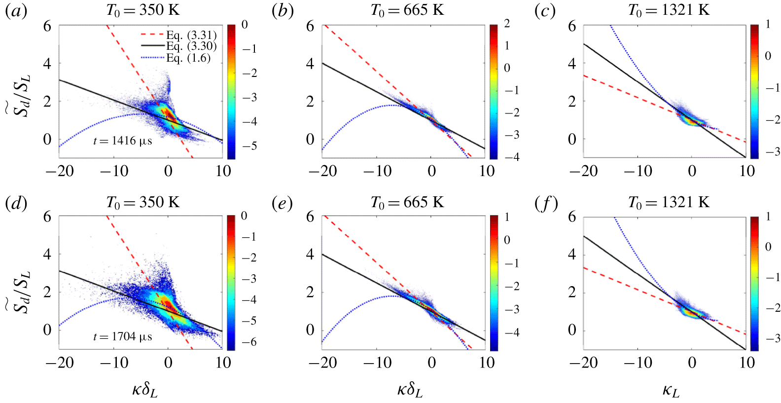
Joint probability density function of one-time instantaneous data of  $\widetilde{S_{d}}/S_{L}$ with respect to normalized stretch rate
 $K\unicode[STIX]{x1D6FF}_{L}/S_{L}$ conditioned on different isotherms. Panels (a–c) relate to Case-L and (d–f) relate to Case-H. The logarithm of the joint probability density is presented in the colour scale. The solid black line shows the prediction from (1.6).

We have also presented the comparison of the DNS data conditioned on instantaneous states of isotherms with the prediction using (1.6). Usually, to study the correlation between  $S_{d}$ and
 $K$, and/or
 $S_{d}$ and
 $\unicode[STIX]{x1D705}$, this is the commonly used approach (Echekki & Chen Reference Echekki and Chen1996; Chen & Im Reference Chen and Im1998, Reference Chen and Im2000; Chakraborty et al. Reference Chakraborty, Klein and Cant2007). Figure 14 shows the joint probability density function ( j.p.d.f.) for
 $\widetilde{S_{d}}/S_{L}$ with respect to
 $K\unicode[STIX]{x1D6FF}_{L}/S_{L}$ conditioned on different isotherms. The logarithm of the probability density values are shown in the colour scale. The first row of figure 14 relates to isotherms from Case-L and the second row relates to Case-H. To make the prediction (solid black line) using (1.6), again a quadratic fit is made between the distribution of stretch rate
 $K$ and curvature
 $\unicode[STIX]{x1D705}$ conditioned on an isotherm, similar to the way in which it was done for figure 13, with the objective to obtain some qualitative insights into the performance of (1.6). The large excursions of
 $\widetilde{S_{d}}$ away from
 $S_{L}$ are not as apparent in figure 14 as they are in figure 13 (DNS data evaluated continuously at the flame particles locations), which can be partly because, in figure 14, joint probability values are presented instead of a scatter. In a j.p.d.f. any realization is presented based on its probability, whereas in a scatter plot a realization is presented without taking its probability into account. Nevertheless, the following things are clearly evident from figure 14 as well. First, one can confidently model the variations in
 $\widetilde{S_{d}}$ in the vicinity of
 $S_{L}$ using the Markstein length theory. Secondly, both
 ${\mathcal{L}}_{K}$ and
 ${\mathcal{L}}_{\unicode[STIX]{x1D705}}$ must be used to capture the effects of stretch and curvature, respectively, and make correct predictions. As such,
 ${\mathcal{L}}_{K}$ and
 ${\mathcal{L}}_{\unicode[STIX]{x1D705}}$ calculated from (1.7) and (1.8), valid in the ‘laminar’ regime, serve the modelling objectives to a large extent. Finally, the third observation is that figures 14(a), 14(b), 14(d) and 14(e) also show that the Markstein length theory predicts incorrect trends for
 $\widetilde{S_{d}}/S_{L}$ in regions of large negative stretch rate. This is evident from the different signs of slope of the black line (positive slope) and the trend that the j.p.d.f.s (negative slope) show for large, negative stretch rates. Only figures 14(c) and 14(f) show a decent agreement between DNS and the model even for large, negative stretch rates. However, as noted earlier,
 ${\mathcal{L}}_{K}$ for the
 $T_{0}=1321~\text{K}$ isotherm is smaller than other isotherms by an order of magnitude. While it is commonly argued that to capture the large excursions of
 $\widetilde{S_{d}}$ away from
 $S_{L}$ one needs to incorporate the stretch effects carefully, it appears that attributing these large excursions to stretch effects has little circumstantial support. Peters (Reference Peters1999) has argued that the effects of diffusive-thermal effects diminish at higher frequency of fluctuations. Clavin & Joulin (Reference Clavin and Joulin1997) have provided some theoretical justification for these conjectures. Experimental studies by Mueller et al. (Reference Mueller, Driscoll, Reuss and Drake1996) show that laminar flames are weakly affected by external stretch rates for a time lag comparable with the chemical time scale. Also, computational studies by Chen & Im (Reference Chen and Im1998) and Im & Chen (Reference Im and Chen2000) give support that the flame speed and stretch-rate correlations are altered due to unsteady effects and the Markstein numbers decrease with increasing frequency. Therefore, given the support from the above studies, we can expect that a flame in all likelihood shows little to no response to stretch effects during rapid transients in Phase-II, and therefore the stretch effects on laminar flames cannot address the large excursions of local
 $S_{d}$ during flame–flame interactions. In summary, figures 11–14 provide enough evidence that applying Markstein length theory for regions of large curvature, which also experience large stretch rates, is likely to produce erroneous estimates. However, the next section gives additional rationale as to why the performance of the Markstein length model quickly deteriorate for Phase-II and articulates the need for a second model. One must note that an important aspect of the Lagrangian-type analysis enabled through the use of flame particles is in its naturalness in separating the two phases of the lifetime of flame particles where the features of variation in
 $\widetilde{S_{d}}$ are distinct. Figure 14 shows that separating such phases is not possible from conditioning variables on an instantaneous realization of an isotherm.
3.3 Phase-II: interaction phase
Two-dimensional contours of temperature (a–c) and heat release rate (d–f) from Case-L at different instants of time  $t$. The solid black line shows the two-dimensional isoline for
 $T_{0}=1321~\text{K}$. The green and the blue coloured boxes are used to highlight the progression of flame–flame interactions locally.

Figure 15 shows two-dimensional contours of temperature and heat-release rate  $\dot{Q}$ from the DNS of Case-L at different instants of time
 $t$ in the first and second rows, respectively. Also, shown in the figure is a line contour for
 $T_{0}=1321~\text{K}$, and two boxes of different edge colour highlighting the progress of two local flame–flame interaction events for a few happening over the duration. Qualitatively, it is evident from the figure that during the flame–flame interactions, which are usually followed by flame annihilation, the local structure of the flame undergoes drastic changes. It is also evident that these transient events have very short time scales. By the time flame–flame interactions are complete, i.e. nearly parallel branches merge (blue box) or pockets form (green box), over a small duration of nearly
 $25~\unicode[STIX]{x03BC}\text{s}$, other non-interacting regions of the flame do not experience any significant change. Thus, different events, such as stretching and flame–flame interactions, on a turbulent premixed flame surface have different time scales. While the non-interacting regions experience straining due to the underlying turbulent flow field and curvature effects, and the time scales of strain rates are of the order of Kolmogorov time scales (Yeung, Girimaji & Pope Reference Yeung, Girimaji and Pope1990), the change in the local flame structure for these non-interacting regions is not drastic in comparison to the change when flame–flame interactions occur. This intimate link between the severity to which the local flame structure is perturbed and level to which
 $\widetilde{S_{d}}$ deviates away from
 $S_{L}$ is explored further in this section.
Schematic detailing the process of defining a local neighbourhood along  $+\boldsymbol{n}^{F}$ and
 $-\boldsymbol{n}^{F}$ up to a distance of
 $2\unicode[STIX]{x1D6FF}_{L}$ on each side. After the local neighbourhood is defined, relevant properties are interpolated to investigate the evolution of flame–flame interaction events.

Comparison of local one-dimensional profiles of  $T$ and
 $Y_{H_{2}}$ obtained from the DNS in the neighbourhood of flame particles with the solution of a standard premixed flame (solid black line). The
 $T$ and
 $Y_{H_{2}}$ profiles at different times are shown using different colours. Profiles at
 $t/\unicode[STIX]{x1D70F}_{F,L}=0.7$, 0.8, 0.95 and 0.99 are presented using solid lines of red, green, blue and magenta colour, respectively. For ease of reference, we have shown the
 $t/\unicode[STIX]{x1D70F}_{F,L}$ values in the vicinity of the corresponding curves in panels ‘
 $a$’ and ‘
 $g$’. These legends apply to the other panels also.

To elaborate the progress of flame–flame interactions, we have also investigated the local structures, both thermal and chemical, in the vicinity of flame particles experiencing such rapid transient events. Figure 16 shows a schematic of how we have investigated the neighbourhood in the vicinity of a flame particle. Point  $A$ qualitatively shows how the local thermal structure in the vicinity of a flame particle in non-interacting regions is expected to be in contrast to a flame particle
 $B$ in the interacting region. First, for each flame particle, we define a set of query points along
 $+\boldsymbol{n}^{F}$ and
 $-\boldsymbol{n}^{F}$. On either side of the flame particle, we define query points up to a distance of
 $2\unicode[STIX]{x1D6FF}_{L}$. Then, we interpolate required variables on these query points at all time instants and analyse the spatial variation of interpolated variables in the normalized time coordinate
 $t/\unicode[STIX]{x1D70F}_{F,L}$. Figures 17(a)–17(c) and figures 17(g)–17(i) show the time evolution of the spatial variation of
 $T$ along the local normal of flame particles on
 $T_{0}=665~\text{K}$ and
 $T_{0}=1321~\text{K}$ isotherms at
 $t/\unicode[STIX]{x1D70F}_{F,L}=$ 0.70, 0.80, 0.95 and 0.99, respectively, along with the spatial variation of
 $T$ in a standard premixed flame (solid black line). These panels corroborate the fact that, as flame particles proceed towards annihilation (
 $t/\unicode[STIX]{x1D70F}_{F,L}\rightarrow 1$) via flame–flame interactions, the local thermal structure in the vicinity of such flame particles changes drastically, and is no longer comparable to the thermal structure of a standard premixed flame. We can similarly conclude that the local chemical structure is drastically altered during these interaction events. Figures 17(d)–17(f) and figures 17(j)–17(l) analyse the time evolution of the spatial variation of
 $Y_{H_{2}}$ along the local normal for the same flame particles, and testifies to this notion. As interaction progresses, the minimum temperature increases towards
 $T_{b}$ and the maximum
 $Y_{H_{2}}$ decreases towards the burned value, leading to the homogenization of the local scalar gradients. Since the flame particles annihilate when their temperature deviates from the level-set value, the temperature at the minima for
 $t/\unicode[STIX]{x1D70F}_{F,L}\approx 1$ in figures 17(a)–17(c) has to be 665 K. This explains why we still observe a significantly deep V-shaped profile for
 $T$ and an inverted V-shaped profile for
 $Y_{H_{2}}$ even at
 $t/\unicode[STIX]{x1D70F}_{F,L}=0.99$ in figures 17(a)–17(f). When same variables are analysed for the flame particles on the
 $T_{0}=1321~\text{K}$ isotherm, we observe that the spatial variations of
 $T$ and
 $Y_{H_{2}}$ at
 $t/\unicode[STIX]{x1D70F}_{F,L}=0.99$ have lesser resemblance to such V-type profiles, and are closer to a near-uniform distribution. We have also extracted heat-release rate
 $\dot{Q}$ profiles along the neighbourhood directed along the local normal of such annihilating flame particles. In view of space, these profiles are not shown here, but before the thermo-diffusive interaction between the approaching flame elements occurs,
 $\dot{Q}$ remains negligible and does not show any change in the upstream region between these interacting flame elements. Even as the interaction proceeds, no homogeneous heat-release region is formed and two distinct peaks in
 $\dot{Q}$ are observed. Therefore, it can be said that the steep acceleration in the
 $\widetilde{S_{d}}$ is a manifestation of flame–flame interactions and not due to some other mechanism, say auto-ignition. These observations on the drastic change in the local flame structure raise serious concerns over extending the concept of Markstein length theory to model
 $\widetilde{S_{d}}$, and justifies the need for a new model to predict
 $\widetilde{S_{d}}$ during flame–flame interactions.
Annihilation of laminar premixed flames undergoing flame–flame interactions has been studied by Chen & Sohrab (Reference Chen and Sohrab1995). The study was numerical and focused primarily on the fundamental aspects of the interaction. Later, Echekki et al. (Reference Echekki, Chen and Gran1996) and Chen et al. (Reference Chen, Echekki and Kollmann1999) studied annihilation due to flame–flame interactions for stoichiometric and lean methane–air turbulent flames using DNS, respectively, and elucidated the annihilation mechanism and stages. Wichman & Vance (Reference Wichman and Vance1997) have examined the governing equations for a one-dimensional model of flame–flame interaction between two identical planar laminar premixed flames, and verified the results with the numerical solution of their model. Subsequently, Lu & Ghosal (Reference Lu and Ghosal2003) developed a similarity solution valid for  $Le=1$, for a similar problem under the constant density assumption. To investigate rapid flame–flame interactions and modelling of the flame speed, we have identified three model problems. The first problem deals with flame–flame interaction between two identical planar premixed flames. For this problem, we have solved the governing equations for both constant density and variable density cases. Please refer to appendix A for the solution. The second model problem deals with an unsteady, inwardly propagating, cylindrical premixed flame. Studies by Pope, Yeung & Girimaji (Reference Pope, Yeung and Girimaji1989), Rutland & Trouvé (Reference Rutland and Trouvé1993) and Uranakara et al. (Reference Uranakara, Chaudhuri, Dave, Arias and Im2016) have shown that the local geometry of the surfaces (material or propagating) interacting with turbulence is predominantly cylindrical. Thus, a laminar cylindrical flame is appropriate to model the geometry of local premixed flame elements in turbulence. Finally, the third model problem involves simplification of the expression for
 $S_{d}$ conditioned on isotherms (1.12), valid under low Mach number conditions derived by neglecting pressure and frictional work terms (Giannakopoulos et al. Reference Giannakopoulos, Gatzoulis, Frouzakis, Matalon and Tomboulides2015; Uranakara et al. Reference Uranakara, Chaudhuri, Dave, Arias and Im2016). The following text discusses the solution of the second and third problems.
Equations (3.8) and (3.9) govern the transient one-dimensional phenomena of an inwardly propagating, cylindrical premixed flame. For this particular problem, we have assumed density to be a constant. In reality, a two-way coupling between the flow field and the flame exists. However, the constant density formulation includes only the effect of the flow field on the flame and not the effect of heat release on the flow. Another implication of the constant density assumption is that the  $S_{d}$ values for different isotherms become comparable, in reality however, it is the density-weighted
 $\widetilde{S_{d}}$ that is comparable across different isotherms. Despite this limitation, the assumption of constant density can help in gathering crucial insights. It has been used in several other studies, such as those by Frankel & Sivashinsky (Reference Frankel and Sivashinsky1984), Mikolaitis (Reference Mikolaitis1984a,Reference Mikolaitisb) and Lu & Ghosal (Reference Lu and Ghosal2003). Apart from constant density, we have also assumed that the thermal conductivity
 $\unicode[STIX]{x1D706}^{\prime }$ and specific heat capacity
 $C_{p}$ are constants and that the gas mixture is initially at rest. Figure 18 shows the schematic of the model problem highlighting the different zones in a premixed flame. Self-interaction begins when the first layer of the preheat zone reaches the centre.
 $$\begin{eqnarray}\displaystyle & \displaystyle \unicode[STIX]{x1D70C}C_{p}\frac{\unicode[STIX]{x2202}T}{\unicode[STIX]{x2202}t}=\frac{1}{r}\frac{\unicode[STIX]{x2202}}{\unicode[STIX]{x2202}r}\left(\unicode[STIX]{x1D706}^{\prime }r\frac{\unicode[STIX]{x2202}T}{\unicode[STIX]{x2202}r}\right)+qw, & \displaystyle\end{eqnarray}$$
 $$\begin{eqnarray}\displaystyle & \displaystyle \unicode[STIX]{x1D70C}\frac{\unicode[STIX]{x2202}Y}{\unicode[STIX]{x2202}t}=\frac{1}{r}\frac{\unicode[STIX]{x2202}}{\unicode[STIX]{x2202}r}\left(\unicode[STIX]{x1D70C}{\mathcal{D}}r\frac{\unicode[STIX]{x2202}Y}{\unicode[STIX]{x2202}r}\right)-w, & \displaystyle\end{eqnarray}$$
where  $q$ is the heat release rate per unit mass of the fuel consumed and
 $w$ is the reaction rate. The boundary conditions for the system of equations are
 $\unicode[STIX]{x2202}T/\unicode[STIX]{x2202}r=0$ and
 $\unicode[STIX]{x2202}Y/\unicode[STIX]{x2202}r=0$ at
 $r=0$ for
 $t\geqslant 0$. Also,
 $T=T_{b}$ and
 $Y=0$ at
 $r=+\infty$ for
 $t\geqslant 0$. When the premixed flame is sufficiently far away from the centre
 $r=0$, the initial condition corresponds to the solution of a steady, inwardly propagating, cylindrical premixed flame.
Schematic of an unsteady, inwardly propagating, cylindrical premixed flame at some time instant.

For the problem described here, we make use of the large activation energy assumption, leading to  $w\approx 0$ in the preheat zone. Consequently, the unsteady and diffusion processes dominate and balance in this zone. To evaluate
 $S_{d}$, first, we transform (3.8) and (3.9) from the
 $r$ coordinate to a stretched coordinate
 $\unicode[STIX]{x1D709}=r/r_{f}$, where
 $r_{f}(t)$ is the radial position of the isotherm of interest at some time
 $t$. Let
 $T_{0}$ be the level-set value of this isotherm located at the boundary between the preheat zone and the reaction zone. In this stretched coordinate, the chosen isotherm
 $T_{0}$ is always located at
 $\unicode[STIX]{x1D709}=1$. The entire event of flame–flame interaction progresses in various stages. Nevertheless, here, we are primarily concerned with the stage or stages where only the preheat zone (thermo-diffusive layers) of the neighbouring elements of a premixed flame interact. We have not analysed the interaction of the reaction zones. We refer to this interaction as the ‘weak’-interaction stage (see Wichman & Vance Reference Wichman and Vance1997). With the assumption
 $w\approx 0$ in the preheat zone, (3.8) decouples from (3.9). Equation (3.10) expresses the temperature equation in the new (
 $t,\unicode[STIX]{x1D709}$) coordinates. The second term, which is a convection-type term on the left-hand side of (3.10), is a result of coordinate transformation from
 $(t,r)$ to
 $(t,\unicode[STIX]{x1D709})$.
 $$\begin{eqnarray}\frac{\unicode[STIX]{x2202}T}{\unicode[STIX]{x2202}t}-\frac{\unicode[STIX]{x1D709}}{r_{f}}\frac{\text{d}r_{f}}{\text{d}t}\frac{\unicode[STIX]{x2202}T}{\unicode[STIX]{x2202}\unicode[STIX]{x1D709}}=\frac{\unicode[STIX]{x1D6FC}_{u}}{r_{f}^{2}}\left[\frac{1}{\unicode[STIX]{x1D709}}\frac{\unicode[STIX]{x2202}T}{\unicode[STIX]{x2202}\unicode[STIX]{x1D709}}+\frac{\unicode[STIX]{x2202}^{2}T}{\unicode[STIX]{x2202}\unicode[STIX]{x1D709}^{2}}\right].\end{eqnarray}$$
Here,  $\text{d}r_{f}/\text{d}t$ is the speed of the isotherm, and our objective is to obtain an expression for it;
 $\unicode[STIX]{x1D6FC}_{u}$ is the thermal diffusivity of the fresh reactants. The boundary conditions for (3.10) are
 $\unicode[STIX]{x2202}T/\unicode[STIX]{x2202}\unicode[STIX]{x1D709}=0$ at
 $\unicode[STIX]{x1D709}=0$ and
 $T=T_{b}$ at
 $\unicode[STIX]{x1D709}=+\infty$. For the isotherm at
 $\unicode[STIX]{x1D709}=1$,
 $T=T_{0}$. Using
 $\unicode[STIX]{x1D703}=(T_{0}-T)/(T_{0}-T_{u})$, we can express (3.10) as given by (3.11). Also,
 $\unicode[STIX]{x1D703}=0$ at
 $\unicode[STIX]{x1D709}=1$ and
 $\unicode[STIX]{x2202}\unicode[STIX]{x1D703}/\unicode[STIX]{x2202}\unicode[STIX]{x1D709}=0$ at
 $\unicode[STIX]{x1D709}=0$.
 $$\begin{eqnarray}\frac{\unicode[STIX]{x2202}\unicode[STIX]{x1D703}}{\unicode[STIX]{x2202}t}-\frac{\unicode[STIX]{x1D709}}{r_{f}}\frac{\text{d}r_{f}}{\text{d}t}\frac{\unicode[STIX]{x2202}\unicode[STIX]{x1D703}}{\unicode[STIX]{x2202}\unicode[STIX]{x1D709}}=\frac{\unicode[STIX]{x1D6FC}_{u}}{r_{f}^{2}}\left[\frac{1}{\unicode[STIX]{x1D709}}\frac{\unicode[STIX]{x2202}\unicode[STIX]{x1D703}}{\unicode[STIX]{x2202}\unicode[STIX]{x1D709}}+\frac{\unicode[STIX]{x2202}^{2}\unicode[STIX]{x1D703}}{\unicode[STIX]{x2202}\unicode[STIX]{x1D709}^{2}}\right].\end{eqnarray}$$
To simplify the notation, we use  $\unicode[STIX]{x1D703}_{t}$ to represent the partial derivative of
 $\unicode[STIX]{x1D703}$ with time, and
 $\unicode[STIX]{x1D703}_{\unicode[STIX]{x1D709}}$ and
 $\unicode[STIX]{x1D703}_{\unicode[STIX]{x1D709}\unicode[STIX]{x1D709}}$ are first and second partial derivatives with
 $\unicode[STIX]{x1D709}$, respectively. Also,
 $\unicode[STIX]{x1D703}_{\unicode[STIX]{x1D709}}(1)$ represents the gradient at
 $\unicode[STIX]{x1D709}=1$. Next, we integrate (3.11) over the domain
 $0\leqslant \unicode[STIX]{x1D709}\leqslant 1$ and simplify to obtain the following equation:
 $$\begin{eqnarray}\int _{0}^{1}\unicode[STIX]{x1D703}_{t}\unicode[STIX]{x1D709}\,\text{d}\unicode[STIX]{x1D709}-\frac{1}{r_{f}}\frac{\text{d}r_{f}}{\text{d}t}\int _{0}^{1}\unicode[STIX]{x1D709}^{2}\unicode[STIX]{x1D703}_{\unicode[STIX]{x1D709}}\,\text{d}\unicode[STIX]{x1D709}=\frac{\unicode[STIX]{x1D6FC}_{u}}{r_{f}^{2}}\unicode[STIX]{x1D703}_{\unicode[STIX]{x1D709}}(1).\end{eqnarray}$$
To estimate the integrals in the equation above, we have assumed the following linear relationship based on Taylor-series expansion:
 $$\begin{eqnarray}\unicode[STIX]{x1D703}_{\unicode[STIX]{x1D709}}(1)\approx \frac{\unicode[STIX]{x1D703}(\unicode[STIX]{x1D709})-0}{\unicode[STIX]{x1D709}-1}.\end{eqnarray}$$
Hence,  $\unicode[STIX]{x1D703}(\unicode[STIX]{x1D709})\approx (\unicode[STIX]{x1D709}-1)\unicode[STIX]{x1D703}_{\unicode[STIX]{x1D709}}(1)$ and
 $\unicode[STIX]{x1D703}_{t}(\unicode[STIX]{x1D709})\approx (\unicode[STIX]{x1D709}-1)\unicode[STIX]{x1D703}_{t\unicode[STIX]{x1D709}}(1)$. Substituting these relationships in (3.12), after simplifying we get
 $$\begin{eqnarray}\frac{\unicode[STIX]{x1D703}_{t\unicode[STIX]{x1D709}}(1)}{6}+\frac{1}{r_{f}}\frac{\text{d}r_{f}}{\text{d}t}\frac{\unicode[STIX]{x1D703}_{\unicode[STIX]{x1D709}}(1)}{3}=-\frac{\unicode[STIX]{x1D6FC}_{u}}{r_{f}^{2}}\unicode[STIX]{x1D703}_{\unicode[STIX]{x1D709}}(1).\end{eqnarray}$$
To obtain an expression for  $\unicode[STIX]{x1D703}_{\unicode[STIX]{x1D709}}(1)$ and
 $\unicode[STIX]{x1D703}_{t\unicode[STIX]{x1D709}}(1)$, we need to analyse the reaction zone. This is done as follows. The reaction zone is extremely thin due to the assumption of large activation energy or large value of
 $\unicode[STIX]{x1D6FD}$, therefore
 $(\unicode[STIX]{x1D706}^{\prime }/r)\unicode[STIX]{x2202}T/\unicode[STIX]{x2202}r\ll \unicode[STIX]{x1D706}^{\prime }\unicode[STIX]{x2202}^{2}T/\unicode[STIX]{x2202}r^{2}$ and can be neglected, and thus the reaction zone is quasi-planar. However, when the reaction zone is curved on of the order of the reaction-zone thickness, then this simplification will not hold further. Integrating (3.8) over the reaction zone gives the following equation:
 $$\begin{eqnarray}\unicode[STIX]{x1D70C}C_{p}r_{f}\int _{r_{f}^{-}}^{r_{f}^{+}}\frac{\unicode[STIX]{x2202}T}{\unicode[STIX]{x2202}t}\,\text{d}r=-\unicode[STIX]{x1D706}^{\prime }r_{f}\int _{r_{f}^{-}}^{r_{f}^{+}}\frac{\unicode[STIX]{x2202}^{2}T}{\unicode[STIX]{x2202}r^{2}}\,\text{d}r+r_{f}\int _{r_{f}^{-}}^{r_{f}^{+}}qw\,\text{d}r.\end{eqnarray}$$
Here  $r_{f}^{-}$ and
 $r_{f}^{+}$ are the upstream (between preheat zone and reaction zone) and downstream (reaction zone and post-flame equilibrium zone) boundaries of the reaction zone. Since the reaction zone is thin,
 $T(r_{f}^{-})\approx T(r_{f}^{+})$, and during the ‘weak’ interactions we can expect the reaction-zone thickness does not change, i.e.
 $\text{d}(r_{f}^{+})/\text{d}t\approx \text{d}(r_{f}^{-})/\text{d}t$. Therefore, using Leibniz’s integral rule it can be shown that
 $$\begin{eqnarray}\int _{r_{f}^{-}}^{r_{f}^{+}}\frac{\unicode[STIX]{x2202}T}{\unicode[STIX]{x2202}t}\,\text{d}r\approx \frac{\text{d}}{\text{d}t}\left(\int _{r_{f}^{-}}^{r_{f}^{+}}T\,\text{d}r\right).\end{eqnarray}$$
Figures 17(a)–17(c) and figures 17(g)–17(i) in this study, and figure 6 and figure 18(a) from the works of Chen & Sohrab (Reference Chen and Sohrab1995) and Minamoto, Yenerdag & Tanahashi (Reference Minamoto, Yenerdag and Tanahashi2018), respectively, show that, during the ‘weak’-interaction phase, the unsteadiness in the average temperature of the reaction zone is not significant. Therefore, from (3.15) and (3.16) it can be said that, during this phase, a balance exists between the diffusion and chemical reactions in the reaction zone. However, during the interaction of the reaction zones, unsteadiness in the reaction zone may no longer be negligible. Therefore, for the quasi-steady, quasi-planar, inner reaction zone, the governing equations are as follows:
 $$\begin{eqnarray}\displaystyle & \displaystyle \unicode[STIX]{x1D706}^{\prime }\frac{\text{d}^{2}T_{in}}{\text{d}r_{in}^{2}}=-qw, & \displaystyle\end{eqnarray}$$
 $$\begin{eqnarray}\displaystyle & \displaystyle \unicode[STIX]{x1D70C}{\mathcal{D}}\frac{\text{d}^{2}Y_{in}}{\text{d}r_{in}^{2}}=w, & \displaystyle\end{eqnarray}$$
where  $w=BY_{in}\exp (-T_{a}/T_{in})$,
 $B$ is the density weighted collision rate of the reaction,
 $T_{a}=E_{a}/R$ is the activation temperature,
 $E_{a}$ is the activation energy and
 $R$ is the universal gas constant. The subscript ‘
 $in$’ is used to denote that the corresponding parameter is analysed over the inner reaction zone.
Following Law (Reference Law2006), we can non-dimensionalize (3.17) and (3.18) using  $\tilde{T}_{in}=C_{p}T_{in}/qY_{u}$,
 ${\tilde{Y}}_{in}=Y_{in}/Y_{u}$ and
 $\tilde{r}_{in}=r_{in}f^{0}C_{p}/\unicode[STIX]{x1D706}^{\prime }$ and simplify the equations to obtain the following expression:
 $$\begin{eqnarray}\left.\left(\frac{\text{d}\tilde{T}_{in}}{\text{d}\tilde{r}_{in}}\right)^{2}\right|_{\tilde{r}_{in}=\tilde{r}_{f}^{-}}=\frac{2Da_{c}^{0}Le}{(\tilde{T_{a}}/\tilde{T}_{b}^{2})^{2}}\text{exp}\left(-\frac{\tilde{T}_{a}}{\tilde{T}_{b}}\right),\end{eqnarray}$$
where  $Da_{c}^{0}=B\unicode[STIX]{x1D706}^{\prime }/f^{0^{2}}C_{p}$. Chung & Law (Reference Chung and Law1988) have shown that
 $T_{b}/T_{b}^{0}=1+\tilde{K}(1/Le-1)$, where
 $T_{b}$ is the burned gas temperature,
 $T_{b}^{0}$ is the adiabatic flame temperature and
 $\tilde{K}$ is the non-dimensional stretch rate. The stretch rate experienced by a cylindrical flame is
 $(1/r_{f})\text{d}r_{f}/\text{d}t$. Therefore, using the expression for
 $T_{b}/T_{b}^{0}$ in (3.19) and ignoring the higher-order terms of
 $\tilde{K}$, it can be shown that
 $\unicode[STIX]{x1D703}_{\unicode[STIX]{x1D709}}(1)=Pr_{f}+Q\,\text{d}r_{f}/\text{d}t$, where
 $P$ and
 $Q$ are constants as shown below,
 $Da^{0}=Da_{c}^{0}\text{exp}(-T_{a}/T_{b}^{0})$ and
 $\unicode[STIX]{x1D6FD}=\tilde{T}_{a}/\tilde{T}_{b}^{0^{2}}$.
 $$\begin{eqnarray}\displaystyle & \displaystyle P=\frac{f^{0}qY_{u}}{(T_{u}-T_{0})\unicode[STIX]{x1D706}^{\prime }}\left(\frac{2Da^{0}Le}{\unicode[STIX]{x1D6FD}^{2}}\right)^{1/2}, & \displaystyle\end{eqnarray}$$
 $$\begin{eqnarray}\displaystyle & \displaystyle Q=\frac{P}{2}\left(4+\frac{T_{a}}{T_{b}^{0}}\right)\left(\frac{1}{Le}-1\right)\frac{\ell _{f}}{S_{L}}. & \displaystyle\end{eqnarray}$$
Substituting  $\unicode[STIX]{x1D703}_{\unicode[STIX]{x1D709}}(1)$ into (3.14) and simplifying, one can obtain the following expression:
 $$\begin{eqnarray}Qr_{f}^{2}\frac{\text{d}^{2}r_{f}}{\text{d}t^{2}}+\frac{\text{d}r_{f}}{\text{d}t}\left(3Pr_{f}^{2}+2Qr_{f}\frac{\text{d}r_{f}}{\text{d}t}+6\unicode[STIX]{x1D6FC}_{u}Q\right)+6\unicode[STIX]{x1D6FC}_{u}Pr_{f}=0.\end{eqnarray}$$
The above equation is a second-order, nonlinear, ordinary differential equation. However, for  $Le=1$,
 $Q=0$ and the above equation can be readily solved to yield the following result:
 $$\begin{eqnarray}\frac{\text{d}r_{f}}{\text{d}t}=-\frac{2\unicode[STIX]{x1D6FC}_{u}}{r_{f}}.\end{eqnarray}$$
Here  $\text{d}r_{f}/\text{d}t=-S_{d}$. Equation (3.23) shows that, as the radius of the curved isotherm reduces, the flame displacement speed tends to infinity. Therefore, as the preheat zones of the flames interact, the isotherm accelerates, and eventually the isotherm vanishes on annihilation. Lu & Ghosal (Reference Lu and Ghosal2003) arrived at similar conclusions for the interaction of two identical planar premixed flames. However, there are some key differences between those results and the results presented here. First, the geometry of the flame considered here is cylindrical and represents a better model for the shape of the flame elements in a turbulent premixed flame. Second, the functional form of the final result is more illuminating. Equation (3.23) expresses a clear relationship between
 $S_{d}$ and the radius
 $r_{f}$, which can be alternatively expressed as shown below, where
 $\unicode[STIX]{x1D705}=-1/r_{f}$.
 $$\begin{eqnarray}S_{d}=-2\unicode[STIX]{x1D6FC}_{u}\unicode[STIX]{x1D705}.\end{eqnarray}$$
Finally, to check the consistency of the models that we have presented for the cylindrical and planar cases (see appendix A), as a third model problem, we have performed a simplification of the expression for  $S_{d}$ conditioned on isotherms (see (1.12)). For this part, we have relaxed the assumption that the thermo-chemical properties, such as
 $\unicode[STIX]{x1D706}^{\prime }$ and
 $C_{p}$, are constants. However, to proceed to the final result we had to use some scaling relationships, which makes the analysis less rigorous. Nevertheless, the functional forms of the solutions of all three problems are consistent with one another. Uranakara et al. (Reference Uranakara, Chaudhuri, Dave, Arias and Im2016) have shown that the contribution of distinct specific heat capacity to
 $S_{d}$, i.e. the second term on the right-hand side of (1.12), is less than the other terms by two orders of magnitude. Additionally, for isotherms sufficiently away from the reaction zone, the third term due to chemical reactions can be ignored when
 $\unicode[STIX]{x1D6FD}$ is large. Therefore, neglecting the second term and third term, (1.12) can be simplified to the following expression:
 $$\begin{eqnarray}S_{d}=\frac{\unicode[STIX]{x1D735}\unicode[STIX]{x1D706}^{\prime }\boldsymbol{\cdot }\unicode[STIX]{x1D735}T}{\unicode[STIX]{x1D70C}C_{p}|\unicode[STIX]{x1D735}T|}+\frac{\unicode[STIX]{x1D706}^{\prime }\unicode[STIX]{x1D735}\boldsymbol{\cdot }\unicode[STIX]{x1D735}T}{\unicode[STIX]{x1D70C}C_{p}|\unicode[STIX]{x1D735}T|}.\end{eqnarray}$$
Assuming  $\unicode[STIX]{x1D706}^{\prime }\sim T$, it can be shown that the numerator of the first term on the right-hand side of (3.25) scales as following
 $\unicode[STIX]{x1D735}\unicode[STIX]{x1D706}^{\prime }\boldsymbol{\cdot }\unicode[STIX]{x1D735}T\sim \unicode[STIX]{x1D735}T\boldsymbol{\cdot }\unicode[STIX]{x1D735}T$. Therefore, the contribution of the first term diminishes as the thermo-diffusive interaction progresses, because
 $|\unicode[STIX]{x1D735}T|\rightarrow 0$. We know that
 $\boldsymbol{n}=-\unicode[STIX]{x1D735}T/|\unicode[STIX]{x1D735}T|$. Therefore, the remaining term in (3.25) can be simplified as follows:
 $$\begin{eqnarray}S_{d}=-\frac{\unicode[STIX]{x1D6FC}}{|\unicode[STIX]{x1D735}T|}\unicode[STIX]{x1D735}\boldsymbol{\cdot }(\boldsymbol{n}|\unicode[STIX]{x1D735}T|),\end{eqnarray}$$
where  $\unicode[STIX]{x1D6FC}$ is the thermal diffusivity conditioned on the isotherm. Simplifying the above equation further, we obtain
 $$\begin{eqnarray}S_{d}=-\unicode[STIX]{x1D6FC}\unicode[STIX]{x1D705}-\frac{\unicode[STIX]{x1D6FC}}{|\unicode[STIX]{x1D735}T|}\boldsymbol{n}\boldsymbol{\cdot }\unicode[STIX]{x1D735}(|\unicode[STIX]{x1D735}T|).\end{eqnarray}$$
Using  $\boldsymbol{n}\boldsymbol{\cdot }\unicode[STIX]{x1D735}=\unicode[STIX]{x2202}/\unicode[STIX]{x2202}n$ and
 $|\unicode[STIX]{x1D735}T|=-\unicode[STIX]{x2202}T/\unicode[STIX]{x2202}n$, where
 $n$ is the coordinate along the local normal, we can express the above equation as follows:
 $$\begin{eqnarray}S_{d}=-\unicode[STIX]{x1D6FC}\unicode[STIX]{x1D705}-\unicode[STIX]{x1D6FC}\frac{\unicode[STIX]{x2202}^{2}T/\unicode[STIX]{x2202}n^{2}}{\unicode[STIX]{x2202}T/\unicode[STIX]{x2202}n}.\end{eqnarray}$$
Now, using simple scaling relationships, such as  $\unicode[STIX]{x2202}^{2}T/\unicode[STIX]{x2202}n^{2}\sim \unicode[STIX]{x0394}T/d^{2}$ and
 $\unicode[STIX]{x2202}T/\unicode[STIX]{x2202}n\sim \unicode[STIX]{x0394}T/d$, it can be shown that the second term on the right-hand side of (3.28) is inversely proportional to
 $d$. The symbol
 $d$ denotes the length scale along the normal coordinate
 $n$. During interaction of thermo-diffusive layers of inwardly propagating cylindrical premixed flames,
 $d$ is the distance from the centre, i.e.
 $d=r_{f}$, and for interacting planar premixed flames,
 $d$ is the distance from the symmetry plane, i.e.
 $d=x_{f}$. Therefore, for the inwardly propagating cylindrical premixed flames, (3.28) can be simplified to
 $\widetilde{S_{d}}=-\unicode[STIX]{x1D6FC}(1+C)\unicode[STIX]{x1D705}\unicode[STIX]{x1D70C}/\unicode[STIX]{x1D70C}_{u}$, where
 $C$ is some scaling constant that needs to determined separately. The above solutions (3.24), (3.28), (A 11) and (A 20) have been determined under the assumptions and boundary conditions of flame–flame interactions such as when
 $\unicode[STIX]{x1D705}\rightarrow \infty$ for curved flames or when the distance between the planar flames goes to zero, i.e.
 $x_{f}\rightarrow 0$. However, these solution derived for the flame–flame interaction limit should match with the solution when the flames are not interacting. Therefore, in the non-interacting limit as
 $\unicode[STIX]{x1D705}\rightarrow 0$ or
 $x_{f}\rightarrow \infty$,
 $\widetilde{S_{d}}\rightarrow S_{L}$ to the leading order. Therefore, the proposed interaction model is as follows:
 $$\begin{eqnarray}\widetilde{S_{d}}=S_{L}-\unicode[STIX]{x1D6FC}(1+C)\unicode[STIX]{x1D705}\unicode[STIX]{x1D70C}/\unicode[STIX]{x1D70C}_{u}.\end{eqnarray}$$
The importance of the contribution of the diffusive term to  $S_{d}$ in a form similar to (3.29) has been recognized by Peters (Reference Peters2000) while deriving an expression for
 $S_{d}$ to be used in the G-equation valid in the thin reaction zone. However, Peters (Reference Peters2000) have not derived the expression to model the propagation during flame–flame interactions and have also ignored the effect of density change on
 $S_{d}$. This is so because, for an isotherm in the inner reaction zone, the sum of the normal and the reaction terms is assumed to be of the order of
 $S_{L}$. Recently, Trivedi et al. (Reference Trivedi, Griffiths, Kolla, Chen and Cant2019a) have also shown that, during pocket formation,
 $S_{d}$ is functionally dependent on the radius
 $r$. However, their analysis was based on Morse theory, which was first used by Chen et al. (Reference Chen, Echekki and Kollmann1999) to study pocket formation in two dimensions, and is conceptually different from the analysis on the three model problems discussed in this study.
An important question that arises now, is regarding the impact that these transient events may have on the other aspects of turbulent premixed flames. Recently, Haghiri et al. (Reference Haghiri, Talei, Brear and Hawkes2018) have found that these flame annihilation events are sources of acoustic sound. They have developed a simple model which employs a condition on  $S_{d}$ to identify the flame annihilation. A discussion on the impact that these flame–flame interaction events can have on the statistics of
 $S_{d}$ is presented in § 4.
3.4 Verification of the interaction model
In this section, we compare the interaction model developed in § 3.3 with the DNS results. First, we compare the model with the DNS data along the flame particle trajectories, followed by comparison with one-time instantaneous data conditioned on the isotherms. To compare (3.29) against the DNS data, we have converted it to the following form using the approximation  $\unicode[STIX]{x1D70C}_{0}/\unicode[STIX]{x1D70C}_{u}\approx T_{u}/T_{0}$, where
 $\unicode[STIX]{x1D70C}_{0}$ is the density conditioned on the isotherm
 $T=T_{0}$.
 $$\begin{eqnarray}\frac{\widetilde{S_{d}}}{S_{L}}=1-\frac{\unicode[STIX]{x1D6FC}}{\unicode[STIX]{x1D703}^{\ast }\unicode[STIX]{x1D6FF}_{L}S_{L}}(1+C)\unicode[STIX]{x1D705}\unicode[STIX]{x1D6FF}_{L}.\end{eqnarray}$$
Time series of  $\widetilde{S_{d}^{F}}/S_{L}$ with respect to normalized curvature
 $\unicode[STIX]{x1D705}^{F}\unicode[STIX]{x1D6FF}_{L}$ evaluated at the flame particle locations. Panels (a–c) relate to Case-L and (d–f) relate to Case-H. The dots represent the time-series data evaluated along the trajectories of all the flame particles. The dots are coloured to show evolution of parameters in normalized time
 $t/\unicode[STIX]{x1D70F}_{F,L}$. The dotted blue line shows prediction from (1.6). The solid black line corresponds to (3.30), assuming
 $C=0.5$. For comparison we have also shown the prediction using (3.31) using a dashed red line.

Figure 19 shows the time series of  $\widetilde{S_{d}^{F}}/S_{L}$ with respect to the normalized curvature
 $\unicode[STIX]{x1D705}^{F}\unicode[STIX]{x1D6FF}_{L}$. (Here
 $\unicode[STIX]{x1D6FF}_{L}=(T_{b}-T_{u})/(\text{d}T/\text{d}x_{max})$ is the thermal thickness and
 $\unicode[STIX]{x1D6FC}_{u}=\ell _{f}S_{L}\neq \unicode[STIX]{x1D6FC}$.) The data are represented with the help of coloured dots for all flame particles from Case-L in the first row and Case-H in the second row. In each panel, we compare the DNS data at the flame particle locations with three important theoretical curves: a black coloured line representing the interaction model (3.30) assuming
 $C=0.5$, a blue coloured dotted curve representing the two-parameter Markstein length model (1.6) and a red coloured dashed line representing prediction using the curvature Markstein length only. While discussing figures 13 and 14, it was already highlighted that using stretch rate as a parameter during flame–flame interactions is not supported based on certain theoretical, experimental and numerical studies and therefore the stretch response of the flame can be considered negligible during flame–flame interactions. Consequently the correction
 ${\mathcal{L}}_{K}K$ can be dropped from (1.6) to get the following ad hoc model. However, it will be shown that, even though the following model incorporates
 $\unicode[STIX]{x1D705}$ as a parameter,
 ${\mathcal{L}}_{\unicode[STIX]{x1D705}}$ is not the correct proportionality constant.
 $$\begin{eqnarray}\frac{\widetilde{S_{d}}}{S_{L}}=1-{\mathcal{L}}_{\unicode[STIX]{x1D705}}\unicode[STIX]{x1D705}.\end{eqnarray}$$
Our focus here is only on the large excursions of  $\widetilde{S_{d}^{F}}$ away from
 $S_{L}$ because we have already established that the mild variations around
 $S_{L}$ can be confidently captured using the two-parameter Markstein length model. Figures 19(a), 19(b), 19(d) and 19(e) clearly show that the trend predicted by (1.6) is inconsistent with, and in fact opposite to the DNS data at the flame particle locations for large negative values of
 $\unicode[STIX]{x1D705}^{F}\unicode[STIX]{x1D6FF}_{L}$. Again, to use (1.6), a nonlinear quadratic fit is made between
 $K^{F}$ and
 $\unicode[STIX]{x1D705}^{F}$, similar to the way it was done for figures 13 and 14. The favourable comparison between (1.6) and the data in figures 19(c) and 19(f) is fortuitous. However, a question may arise concerning why
 ${\mathcal{L}}_{\unicode[STIX]{x1D705}}$ cannot be an appropriate proportionality constant if curvature is an important parameter during the interaction of curved flame elements. As can be seen from table 2 and the work of Giannakopoulos et al. (Reference Giannakopoulos, Gatzoulis, Frouzakis, Matalon and Tomboulides2015),
 ${\mathcal{L}}_{\unicode[STIX]{x1D705}}$ decreases from large values near the fresh reactants to zero near the burned products. Each row in figure 19, therefore, shows that the slope of the red dashed line reduces as
 $T_{0}$ increases and moves in the direction opposite to the slope of the DNS data at the flame particle locations. These observations establish the limitation of two-parameter Markstein length model and even its individual components in modelling
 $\widetilde{S_{d}}$ during flame–flame interactions. Finally, it can be seen that the prediction based on the interaction model, i.e. the solid black line, is able to capture the dominant trends of large excursions of
 $\widetilde{S_{d}^{F}}$ away from
 $S_{L}$ in each panel. In figures 19(c) and 19(f), the slight discrepancy between the interaction model and the DNS data at the flame particle locations can be attributed to the simplifying assumptions under which the interaction model has been derived. It only accounts for the preheat zone interactions with reaction zones localized near the burned side. However, a DNS of a premixed flame with a detailed reaction mechanism for an
 $\text{H}_{2}$–air mixture has heat release nearly over the entire width of the flame.
Joint probability density function of one-time instantaneous data of  $\widetilde{S_{d}}/S_{L}$ with respect to normalized curvature
 $\unicode[STIX]{x1D705}\unicode[STIX]{x1D6FF}_{L}$ conditioned on different isotherms. Panels (a–c) relate to Case-L and (d–f) relate to Case-H. The natural logarithm of the joint probability density is presented in the colour scale. The solid black line shows prediction from (1.6). The solid blue line corresponds to (3.30), assuming
 $C=0.5$. For comparison we have also shown the line using the curvature Markstein length alone (1.8).

Joint probability density function of one-time instantaneous data of  $\widetilde{S_{d}}/S_{L}$ with respect to normalized curvature
 $\unicode[STIX]{x1D705}\unicode[STIX]{x1D6FF}_{L}$ conditioned on different isotherms. Except for time instants at which these j.p.d.f.s are made, all other features of this figure are identical to figure 20.

Finally, figure 20 shows the j.p.d.f. of  $\widetilde{S_{d}}/S_{L}$ and
 $\unicode[STIX]{x1D705}\unicode[STIX]{x1D6FF}_{L}$ conditioned on an instantaneous state of different isotherms. For Case-L (figure 20a–c)
 $t=1341~\unicode[STIX]{x03BC}\text{s}$ is chosen while for Case-H (figure 20d–f)
 $t=1500~\unicode[STIX]{x03BC}\text{s}$ is used. The figure also shows the comparison of the j.p.d.f. with three theoretical curves: a black curve representing the predictions from (3.30), a dotted blue curve representing prediction from (1.6) and a dashed red line showing the predictions using (3.31). Again, to plot the dotted blue curve,
 $K$ and
 $\unicode[STIX]{x1D705}$ are conditioned on an isotherm and a nonlinear quadratic fit is made between the distributions of
 $K$ and
 $\unicode[STIX]{x1D705}$ for that isotherm, similar to the way it was done for figure 14. On comparing figures 19 and 20, we can make the following observations. Our focus again is only on the large excursions of
 $\widetilde{S_{d}}$ away from
 $S_{L}$. The first observation is that the two-parameter Markstein length model (1.6) fails to model the dominant trends of
 $\widetilde{S_{d}}$ in regions of large, negative
 $\unicode[STIX]{x1D705}$, except for figures 20(c) and 20(f) where (1.6) decently captures the trend. However, the comparison is termed fortuitous for the following reasons. It is evident from the results in this study and also from the work of Chen et al. (Reference Chen, Echekki and Kollmann1999),
 $\widetilde{S_{d}}>0$ and is very large during the flame–flame interactions. The stretch rate
 $K$ during such events is negative (
 $K<0$) and large in magnitude, as after interaction flame elements usually annihilate. Therefore, if we are on isotherms closer to the burned products such that
 ${\mathcal{L}}_{\unicode[STIX]{x1D705}}\rightarrow 0$ then to allow
 $\widetilde{S_{d}}>0$ provided that
 $K<0$, the stretch Markstein length should always be positive, i.e.
 ${\mathcal{L}}_{K}>0$. This puts a restriction on the values that
 ${\mathcal{L}}_{K}$ can take for isotherms near the burned products. However,
 ${\mathcal{L}}_{K}$ is known to attain both positive and negative values. For example, figure 7.6.6 from Law (Reference Law2006) shows that the Markstein length evaluated on the burned side for lean (
 $\unicode[STIX]{x1D719}=0.6$) and rich (
 $\unicode[STIX]{x1D719}=3.0$)
 $\text{H}_{2}$–air premixed flames at
 $P=1~\text{atm}$ is negative and positive, respectively. These arguments give additional support to why the Markstein length type models are not applicable during flame–flame interactions. Also, the trend of
 $\widetilde{S_{d}}/S_{L}$ predicted in figures 20(a), 20(b), 20(d) and 20(e) is opposite to the trends that the j.p.d.f.s show for large, negative
 $\unicode[STIX]{x1D705}$. Figure 21 shows the j.p.d.f. similar to figure 20. The only difference between the two figures is the time instant at which the instantaneous j.p.d.f.s are constructed. Figure 21 shows that the observations that the two-parameter Markstein length model is inadequate to predict
 $\widetilde{S_{d}}$ during flame–flame interactions and that the interaction model is required to predict
 $\widetilde{S_{d}}$ during such interactions is corroborated further with the j.p.d.f.s for each case at two different time instants. Now, even if we ignore the contribution of
 $K$ due to small time scales of the interaction events, as argued towards the end of § 3.2, and drop the second term from (1.6) and use only
 ${\mathcal{L}}_{\unicode[STIX]{x1D705}}$ to incorporate the dependence of
 $\widetilde{S_{d}}$ on
 $\unicode[STIX]{x1D705}$, the red dashed line representing these approximations fails to capture the large excursions of
 $\widetilde{S_{d}}$ away from
 $S_{L}$. In fact, the slope of the red line moves in the direction opposite to the trend that the j.p.d.f.s show for large, negative
 $\unicode[STIX]{x1D705}$. On the contrary, the interaction model (black solid line) can indeed capture the large excursions of
 $\widetilde{S_{d}}$ in the interacting regions. It makes good quantitative predictions for two isotherms and is qualitatively consistent with the trends that the j.p.d.f.s display for the remaining cases. Second, the variation of
 $\widetilde{S_{d}}$ during the rapid flame–flame interaction events is clearly captured when the DNS data are continuously evaluated at the flame particle locations (figure 19) in contrast to the instantaneous data (figure 20). This is because, as
 $t/\unicode[STIX]{x1D70F}_{F,L}\rightarrow 1$, all the flame particles annihilate, while at a given time instant
 $t$ not many regions of a turbulent premixed flame may be experiencing such interactions, resulting in a lower probability density. However, implication of such events may be stronger for turbulent premixed flames at higher Karlovitz number. This highlights the significance of Lagrangian-type analyses like FFPT and BFPT algorithms in capturing certain features of turbulent premixed flames which otherwise may remain obscure when data are conditioned on instantaneous states of isotherms. Therefore, figures 19 and 20 provide sufficient support for the interaction model that can be used to predict the large excursions of
 $\widetilde{S_{d}}$ away from
 $S_{L}$ when the flame elements experience interaction with other regions of the flame.
4 Implications for flame displacement speed models
An important outcome of this study is that it provides unprecedented support for the two-parameter Markstein length model in modelling the variations in  $\widetilde{S_{d}}$ away from
 $S_{L}$ even for turbulent premixed flames with
 $Ka$ of 18. However, the study also shows that the two-parameter Markstein length theory should be applied with care. In regions of flame–flame interaction, large deviations in
 $\widetilde{S_{d}}$ occur and these cannot be captured by the model. We have then proposed a new model to capture the large excursions
 $\widetilde{S_{d}}$ away from
 $S_{L}$. The interaction model, which shows
 $S_{d}$ to be functionally related to the curvature for interacting curved flames, is able to capture the dominant features which are not explained by the first model. First, it would be of interest to see how to switch between the Markstein length model and the interaction model. One suggested criterion, without analysis, can be to identify interacting and non-interacting regions based on curvature. If the flame is curved inwards with local radius of curvature lesser than the thermal thickness of the flame, say
 $\unicode[STIX]{x1D6FF}_{L}$, then the probability of flame–flame interactions is high. One can then use the interaction model for such regions with
 $\unicode[STIX]{x1D705}\unicode[STIX]{x1D6FF}_{L}<-1$ whereas for other regions the two-parameter Markstein length model should be used. One must note that the suggested segregation criterion does not take into account planar flame–flame interactions. A demonstration of the simultaneous use of the two models will be taken up in the future. Moreover, it would be of interest to see how the interaction model performs for larger values of turbulent flame intensity
 $u_{0}/S_{L}$, high Karlovitz number (Nilsson et al. Reference Nilsson, Carlsson, Yu and Bai2018) and elevated pressures. Certain studies, such as by Trivedi, Nivarti & Cant (Reference Trivedi, Nivarti and Cant2019b), have shown that more flame–flame interactions occur when the turbulent intensity is increased. Another natural extension of this work would be to test these two models simultaneously to predict the turbulent flame speed
 $S_{T}$. Predictions of local
 $S_{d}$ from the two models can be appropriately averaged to determine
 $S_{T}$. The following equation shows how
 $S_{T}$ is related to
 $\widetilde{S_{d}}$:
 $$\begin{eqnarray}S_{T}=\frac{1}{A_{L}}\int _{A_{T}}\widetilde{S_{d}}\,\text{d}A,\end{eqnarray}$$
where  $A_{T}$ is the turbulent flame surface area and
 $A_{L}$ is the projected flame area. According to Damköhler’s first hypothesis, the increase in
 $S_{T}$ is primarily due to the wrinkling of the flame surface. Through the two-parameter Markstein length model we now know that flame responds to stretch and curvature effects with the sensitivity controlled through the Markstein lengths. Therefore, it is not difficult to anticipate that the response of flame to stretch and curvature effects will constitute secondary influences. However, this study shows that the flame–flame interaction events can also feature in as a new phenomenon that can affect
 $S_{T}$. While interaction events are properly captured by the analysis of DNS data at the flame particles in normalized time coordinate, the analysis where data are conditioned on instantaneous states of the isotherm show that the probability of such events at a given time instant
 $t$ is low. But, as highlighted above,
 $u_{0}/S_{L}$,
 $Ka$ and pressure can influence this probability. Therefore, an assessment of the bearing that these flame–flame interaction events will have on
 $S_{T}$ and the factors that modulate these interaction events will be taken up as a future work.
5 Conclusions
Modelling flame speeds in turbulent premixed flames is a challenge. A common approach is to use models developed for stretched laminar flames to understand turbulent premixed flames. A model by Giannakopoulos et al. (Reference Giannakopoulos, Gatzoulis, Frouzakis, Matalon and Tomboulides2015) based on the originally proposed one by Bechtold & Matalon (Reference Bechtold and Matalon2001) show that the density-weighted flame displacement speed  $\widetilde{S_{d}}$ conditioned on isotherms representing a flame is a function of two parameters: stretch rate
 $K$ and curvature
 $\unicode[STIX]{x1D705}$, and that two distinct Markstein lengths exist. This study presents an assessment of its applicability to model
 $\widetilde{S_{d}}$ in turbulent premixed flames locally at many points on different isotherms, for the first time. We have performed DNS of
 $\text{H}_{2}$–air turbulent premixed flames with detailed chemistry and analysed two DNS cases in the thin reaction zone regime. With the help of a Lagrangian-type analysis, enabled through the use of flame particles, we have shown that the two-parameter Markstein length model is adequate to model the mild and gradual variations of
 $\widetilde{S_{d}}$ in the vicinity of laminar flame speed
 $S_{L}$, for most parts of the flame. However, the model is unacceptable in regions where flame–flame interactions occur and
 $\widetilde{S_{d}}$ displays large excursions away from
 $S_{L}$. We have developed a new interaction model to capture these large excursions.
Tracking flame particles provides us with spatio-temporal details of local states of turbulent premixed flames. Using backward flame particle tracking followed by forward flame particle tracking, we have traced the trajectories of flame particles over their entire lifetime – from generation to annihilation. This helps in creating a manifold of local states with which we can assess any state of any point on a turbulent premixed flame, under the same inlet and ambient conditions. Time series of  $\widetilde{S_{d}}$ evaluated directly from the DNS at the flame particle locations show two broad features. For approximately 80 % of flame particle lifetime, the variations in
 $\widetilde{S_{d}}$ are mild and gradual. This is referred to as the non-interaction phase or Phase-I. For this phase, the two-parameter Markstein length model is adequate to explain variations in
 $\widetilde{S_{d}}$, both quantitatively and qualitatively. The local thermal and chemical structures in the neighbourhood of flame particles are comparable to corresponding profiles from a standard premixed flame. Analysis of the spatial location of flame particles shows that, during Phase-I, flame particles predominantly occupy regions which do not experience interaction with other regions of the flame and are largely affected by stretch and curvature effects. In contrast, when the two-parameter Markstein length model is assessed for the remaining 20 % of flame particle lifetime, the error between the model predictions and DNS is unacceptable. Thus, flame particle tracking methods provide a natural and convenient means for segregating phases in lifetime of flame particles and consequently spatial regions on a turbulent premixed flame where the two-parameter Markstein length model holds and does not hold.
The remaining 20 % of flame particle lifetime is referred to as the interacting phase, or Phase-II. During this phase, flame particles predominantly occupy regions with large, negative curvature  $\unicode[STIX]{x1D705}$ (curved concave to fresh reactants). Flame–flame interactions between neighbouring elements of a finitely thick flame become increasingly probable as
 $\unicode[STIX]{x1D705}$ becomes large and negative. Since these interactions are usually followed by local annihilation of flame surfaces,
 $K$ is also large and negative for such regions. Due to these flame–flame interactions, the local thermal and chemical structure is significantly altered over a very small time scale and transients become extremely important. Establishing this crucial link between the severity to which the local flame structure is perturbed and the level to which
 $\widetilde{S_{d}}$ deviates away from
 $S_{L}$ was made possible by use of flame particle tracking methods. The j.p.d.f.s, which are one-time
 $n$-point statistics, cannot capture the dynamics of such interaction events adequately. To model the evolution of
 $\widetilde{S_{d}}$ during this phase, we have solved three simple model problems: interaction of two identical planar premixed flames, an unsteady, inwardly propagating, cylindrical premixed flame and an analysis of the expression of flame displacement speed conditioned on isotherms. The solutions show that, irrespective of the flame geometry, as the flame–flame interaction events occur, the flame accelerates and
 $\widetilde{S_{d}}$ becomes very large, prior to annihilation;
 $\widetilde{S_{d}}$ is proportional to the inverse of radius (or directly to curvature) for curved interactions, or to the inverse of the distance from the symmetry plane for planar interactions. The interaction model is verified against the DNS data processed using two different approaches: evaluation of time series at flame particle locations and j.p.d.f.s. The interaction model so developed in this study is able to explain the dominant features of large excursions of
 $\widetilde{S_{d}}$ seen in data from each of these viewpoints. Thus, with the help of flame particle tracking, this study addresses a long-standing concern on modelling flame displacement speed for turbulent premixed flames. We show that simultaneous use of two models – a two-parameter Markstein length model to explain the mild and gradual variations of
 $\widetilde{S_{d}}$ near
 $S_{L}$ and an interaction model to explain the large excursions of
 $\widetilde{S_{d}}$ away from
 $S_{L}$ – is required to explain and model flame displacement speeds of premixed flames in turbulence.
Acknowledgements
We sincerely acknowledge the associate editor Professor M. Matalon and the anonymous reviewers for their comments on this paper. The DNS reported in this paper were performed on the Cray XC-40 at the Supercomputer Education and Research Centre (SERC), Indian Institute of Science, Bangalore. H.L.D. would also like to acknowledge financial assistance by the Government of India through the MHRD scholarships.
Appendix A. Solution for thermo-diffusive interactions of planar premixed flames: constant and variable density cases
Here we have presented the solution for the thermo-diffusive interactions of two mutually colliding planar premixed flames. We have performed the analysis for both the constant density and variable density cases. First, we discuss the case where density is assumed constant and the gas mixture is at rest initially. Equations (A 1)–(A 2) are the governing equations for temperature and species.
 $$\begin{eqnarray}\displaystyle & \displaystyle \unicode[STIX]{x1D70C}C_{p}\frac{\unicode[STIX]{x2202}T}{\unicode[STIX]{x2202}t}=\frac{\unicode[STIX]{x2202}}{\unicode[STIX]{x2202}x}\left(\unicode[STIX]{x1D706}^{\prime }\frac{\unicode[STIX]{x2202}T}{\unicode[STIX]{x2202}x}\right)+qw, & \displaystyle\end{eqnarray}$$
 $$\begin{eqnarray}\displaystyle & \displaystyle \unicode[STIX]{x1D70C}\frac{\unicode[STIX]{x2202}Y}{\unicode[STIX]{x2202}t}=\frac{\unicode[STIX]{x2202}}{\unicode[STIX]{x2202}x}\left(\unicode[STIX]{x1D70C}{\mathcal{D}}\frac{\unicode[STIX]{x2202}Y}{\unicode[STIX]{x2202}x}\right)-w. & \displaystyle\end{eqnarray}$$
Figure 22 shows a schematic of the set-up for the problem of mutual collision of identical planar premixed flames. A symmetry plane exists at  $x=0$. The boundary conditions are
 $\unicode[STIX]{x2202}T/\unicode[STIX]{x2202}x=0$ and
 $\unicode[STIX]{x2202}Y/\unicode[STIX]{x2202}x=0$ at
 $x=0$ and
 $T=T_{b}$ and
 $Y=0$ at
 $x=+\infty$ for
 $t\geqslant 0$. When the flames are sufficiently far from the symmetry plane at
 $x=0$, the initial conditions for
 $T$ and
 $Y$ correspond to the solution of a standard premixed flame. Similar to the discussion in § 3.3, let
 $T_{0}$ be the isotherm of interest located initially at
 $x=x_{f}$ situated at the boundary between the preheat zone and the reaction zone. Under the assumption of large activation energy, we can assume that
 $w\approx 0$ in the preheat zone. Consequently, the temperature equation (A 1) gets decoupled from the species transport equation (A 2), and a balance exists between the unsteady effect and the diffusion effect in the preheat zone during the ‘weak’ interaction. Next, we transform the temperature equation from the
 $(t,x)$ coordinates to
 $(t,\unicode[STIX]{x1D709})$, where
 $\unicode[STIX]{x1D709}=x/x_{f}$ is a stretched coordinate. The transformed temperature equation is as shown below.
 $$\begin{eqnarray}\frac{\unicode[STIX]{x2202}T}{\unicode[STIX]{x2202}t}-\frac{\unicode[STIX]{x1D709}}{x_{f}}\frac{\text{d}x_{f}}{\text{d}t}\frac{\unicode[STIX]{x2202}T}{\unicode[STIX]{x2202}\unicode[STIX]{x1D709}}=\frac{\unicode[STIX]{x1D6FC}_{u}}{x_{f}^{2}}\frac{\unicode[STIX]{x2202}^{2}T}{\unicode[STIX]{x2202}\unicode[STIX]{x1D709}^{2}}.\end{eqnarray}$$
Using  $\unicode[STIX]{x1D703}=(T_{0}-T)/(T_{0}-T_{u})$ and the short-hand notation for representing partial derivatives, as discussed previously, we can express the governing equation for reduced temperature
 $\unicode[STIX]{x1D703}$ in the new coordinates using the following equation:
 $$\begin{eqnarray}\unicode[STIX]{x1D703}_{t}-\frac{\unicode[STIX]{x1D709}}{x_{f}}\frac{\text{d}x_{f}}{\text{d}t}\unicode[STIX]{x1D703}_{\unicode[STIX]{x1D709}}=\frac{\unicode[STIX]{x1D6FC}_{u}}{x_{f}^{2}}\unicode[STIX]{x1D703}_{\unicode[STIX]{x1D709}\unicode[STIX]{x1D709}}.\end{eqnarray}$$
A schematic for the one-dimensional model for collision of two identical planar premixed flame. This model is used for the investigation of flame speed when the thermo-diffusive interactions progress during flame–flame collision.

Integrating the above equation from  $\unicode[STIX]{x1D709}=0$ to
 $\unicode[STIX]{x1D709}=1$ and simplifying, we get the following equation:
 $$\begin{eqnarray}\int _{0}^{1}\unicode[STIX]{x1D703}_{t}\,\text{d}\unicode[STIX]{x1D709}+\frac{1}{x_{f}}\frac{\text{d}x_{f}}{\text{d}t}\int _{0}^{1}\unicode[STIX]{x1D703}\,\text{d}\unicode[STIX]{x1D709}=\frac{\unicode[STIX]{x1D6FC}_{u}}{x_{f}^{2}}\unicode[STIX]{x1D703}_{\unicode[STIX]{x1D709}}(1),\end{eqnarray}$$
where  $\unicode[STIX]{x1D703}_{\unicode[STIX]{x1D709}}(1)$ is the gradient at the isotherm
 $T=T_{0}$ or
 $\unicode[STIX]{x1D703}=0$ at
 $\unicode[STIX]{x1D709}=1$. To estimate the integrals in the equation above, we use the approximations
 $\unicode[STIX]{x1D703}(\unicode[STIX]{x1D709})=(\unicode[STIX]{x1D709}-1)\unicode[STIX]{x1D703}_{\unicode[STIX]{x1D709}}(1)$ and
 $\unicode[STIX]{x1D703}_{t}=(\unicode[STIX]{x1D709}-1)\unicode[STIX]{x1D703}_{t\unicode[STIX]{x1D709}}(1)$. Substituting these relationships in (A 5), we get the following relationship:
 $$\begin{eqnarray}\frac{\unicode[STIX]{x1D703}_{t\unicode[STIX]{x1D709}}(1)}{2}+\frac{1}{x_{f}}\frac{\text{d}x_{f}}{\text{d}t}\frac{\unicode[STIX]{x1D703}_{\unicode[STIX]{x1D709}}(1)}{2}=-\frac{\unicode[STIX]{x1D6FC}_{u}}{x_{f}^{2}}\unicode[STIX]{x1D703}_{\unicode[STIX]{x1D709}}(1).\end{eqnarray}$$
To obtain a relationship for  $\unicode[STIX]{x1D703}_{t\unicode[STIX]{x1D709}}(1)$ and
 $\unicode[STIX]{x1D703}_{\unicode[STIX]{x1D709}}(1)$, we have to analyse the reaction zone. In the reaction zone, as argued earlier, the diffusion and the reaction effects dominate and balance each other. Therefore, in the quasi-steady, inner reaction zone, equations (A 1) and (A 2) simplify to the following set of equations:
 $$\begin{eqnarray}\displaystyle & \displaystyle \unicode[STIX]{x1D706}^{\prime }\frac{\text{d}^{2}T_{in}}{\text{d}x_{in}^{2}}=-qw, & \displaystyle\end{eqnarray}$$
 $$\begin{eqnarray}\displaystyle & \displaystyle \unicode[STIX]{x1D70C}{\mathcal{D}}\frac{\text{d}^{2}Y_{in}}{\text{d}x_{in}^{2}}=w, & \displaystyle\end{eqnarray}$$
where  $w=BY_{in}\exp (-T_{a}/T_{in})$. Following Law (Reference Law2006), one can use non-dimensional parameters like
 $\tilde{T}_{in}=C_{p}T_{in}/qY$,
 ${\tilde{Y}}_{in}=Y_{in}/Y_{u}$ and
 $\tilde{x}_{in}=x_{in}f^{0}C_{p}/\unicode[STIX]{x1D706}^{\prime }$ to obtain the following relationship:
 $$\begin{eqnarray}\left.\left(\frac{\text{d}\tilde{T}_{in}}{\text{d}\tilde{x}_{in}}\right)^{2}\right|_{\tilde{x}_{in}=\tilde{x}_{f}}=\frac{2Da^{0}Le}{\unicode[STIX]{x1D6FD}^{2}}.\end{eqnarray}$$
Therefore, we can define  $\unicode[STIX]{x1D703}_{\unicode[STIX]{x1D709}}(1)=Ax_{f}$ and
 $\unicode[STIX]{x1D703}_{t\unicode[STIX]{x1D709}}(1)=A\text{d}x_{f}/\text{d}t$, where
 $A$ is given as follows:
 $$\begin{eqnarray}A=\frac{f^{0}qY_{u}}{(T_{u}-T_{0})\unicode[STIX]{x1D706}^{\prime }}\left(\frac{2Da^{0}Le}{\unicode[STIX]{x1D6FD}^{2}}\right)^{1/2}.\end{eqnarray}$$
Substituting  $\unicode[STIX]{x1D703}_{\unicode[STIX]{x1D709}}(1)$ and
 $\unicode[STIX]{x1D703}_{t\unicode[STIX]{x1D709}}(1)$ into (A 6) and simplifying, one can obtain the following relationship:
 $$\begin{eqnarray}\frac{\text{d}x_{f}}{\text{d}t}=-\frac{\unicode[STIX]{x1D6FC}_{u}}{x_{f}}.\end{eqnarray}$$
The final form of (A 11) closely resembles (3.23), except for the constant. However, one must take a note of the subtle differences, here  $x_{f}$ is the distance of the isotherm from the symmetry plane and
 $\text{d}x_{f}/\text{d}t=-S_{d}$. The above equation also predicts that
 $S_{d}$ for an isotherm runs over to infinity as the two premixed flames collide and progress through thermo-diffusive interactions. Therefore, the feature of flame acceleration during thermo-diffusive interactions is salient irrespective of the geometry of the flame.
While assuming density to be a constant can drastically simplify the problem and make the analysis tractable, it also removes the effect of heat release on the flow field. To assess whether this assumption has any significant bearing on the final result, we have also solved the case where density is variable. The following system of equations governs the phenomena when density is not a constant. The set-up of the problem is same as that described for the constant density case.
 $$\begin{eqnarray}\displaystyle & \displaystyle \frac{\unicode[STIX]{x2202}\unicode[STIX]{x1D70C}}{\unicode[STIX]{x2202}t}+\frac{\unicode[STIX]{x2202}(\unicode[STIX]{x1D70C}u)}{\unicode[STIX]{x2202}x}=0, & \displaystyle\end{eqnarray}$$
 $$\begin{eqnarray}\displaystyle & \displaystyle \unicode[STIX]{x1D70C}C_{p}\frac{\unicode[STIX]{x2202}T}{\unicode[STIX]{x2202}t}+\unicode[STIX]{x1D70C}uC_{p}\frac{\unicode[STIX]{x2202}T}{\unicode[STIX]{x2202}x}=\frac{\unicode[STIX]{x2202}}{\unicode[STIX]{x2202}x}\left(\unicode[STIX]{x1D706}^{\prime }\frac{\unicode[STIX]{x2202}T}{\unicode[STIX]{x2202}x}\right)+qw, & \displaystyle\end{eqnarray}$$
 $$\begin{eqnarray}\displaystyle & \displaystyle \unicode[STIX]{x1D70C}\frac{\unicode[STIX]{x2202}Y}{\unicode[STIX]{x2202}t}+\unicode[STIX]{x1D70C}u\frac{\unicode[STIX]{x2202}Y}{\unicode[STIX]{x2202}x}=\frac{\unicode[STIX]{x2202}}{\unicode[STIX]{x2202}x}\left(\unicode[STIX]{x1D70C}{\mathcal{D}}\frac{\unicode[STIX]{x2202}Y}{\unicode[STIX]{x2202}x}\right)-w. & \displaystyle\end{eqnarray}$$
Following Wichman & Vance (Reference Wichman and Vance1997), we select a new Lagrangian coordinate  $z=\int _{0}^{x}\unicode[STIX]{x1D70C}\,\text{d}q$, where
 $\unicode[STIX]{x2202}z/\unicode[STIX]{x2202}t=-\unicode[STIX]{x1D70C}u$ and
 $\unicode[STIX]{x2202}z/\unicode[STIX]{x2202}x=\unicode[STIX]{x1D70C}$. As discussed by Spalding (Reference Spalding1956), the new coordinate can be chosen such that there is no net mass flow across planes of equal
 $z$. In this new coordinate, the convection term drops out from each equation, and the continuity equation is automatically satisfied. This transformation has also been used by Bledjian (Reference Bledjian1973). The governing equations in the new
 $(t,z)$ coordinates are as follows:
 $$\begin{eqnarray}\displaystyle & \displaystyle \unicode[STIX]{x1D70C}C_{p}\frac{\unicode[STIX]{x2202}T}{\unicode[STIX]{x2202}t}=\unicode[STIX]{x1D70C}\frac{\unicode[STIX]{x2202}}{\unicode[STIX]{x2202}z}\left(\unicode[STIX]{x1D70C}\unicode[STIX]{x1D706}^{\prime }\frac{\unicode[STIX]{x2202}T}{\unicode[STIX]{x2202}z}\right)+qw, & \displaystyle\end{eqnarray}$$
 $$\begin{eqnarray}\displaystyle & \displaystyle \unicode[STIX]{x1D70C}\frac{\unicode[STIX]{x2202}Y}{\unicode[STIX]{x2202}t}=\unicode[STIX]{x1D70C}\frac{\unicode[STIX]{x2202}}{\unicode[STIX]{x2202}z}\left(\unicode[STIX]{x1D70C}^{2}{\mathcal{D}}\frac{\unicode[STIX]{x2202}Y}{\unicode[STIX]{x2202}z}\right)-w. & \displaystyle\end{eqnarray}$$
Since  $\unicode[STIX]{x1D70C}\sim 1/T$ and
 $\unicode[STIX]{x1D706}^{\prime }\sim T$, we can assume
 $\unicode[STIX]{x1D70C}\unicode[STIX]{x1D706}^{\prime }$ as a constant. Also, we have assumed
 $C_{p}$ to be a constant. Again using the large activation energy assumption, we can assume
 $w\approx 0$ in the preheat zone and decouple the temperature (A 15) and the species transport (A 16) equations. Now, we define a new stretched coordinate
 $\unicode[STIX]{x1D709}=z/z_{f}$. The transformed equation for temperature in the new
 $(t,\unicode[STIX]{x1D709})$ coordinates is as follows:
 $$\begin{eqnarray}\frac{\unicode[STIX]{x2202}T}{\unicode[STIX]{x2202}t}-\frac{\unicode[STIX]{x1D709}}{z_{f}}\frac{\text{d}z_{f}}{\text{d}t}\frac{\unicode[STIX]{x2202}T}{\unicode[STIX]{x2202}\unicode[STIX]{x1D709}}=\frac{k_{u}}{z_{f}^{2}}\frac{\unicode[STIX]{x2202}^{2}T}{\unicode[STIX]{x2202}\unicode[STIX]{x1D709}^{2}},\end{eqnarray}$$
where  $k_{u}=\unicode[STIX]{x1D70C}_{u}\unicode[STIX]{x1D706}_{u}/C_{p,u}$. Using
 $\unicode[STIX]{x1D703}=(T_{0}-T)/(T_{0}-T_{u})$, and following the short-hand notation as used earlier, we can express the above equation as.
 $$\begin{eqnarray}\unicode[STIX]{x1D703}_{t}-\frac{\unicode[STIX]{x1D709}}{z_{f}}\frac{\text{d}z_{f}}{\text{d}t}\unicode[STIX]{x1D703}_{\unicode[STIX]{x1D709}}=\frac{k_{u}}{z_{f}^{2}}\unicode[STIX]{x1D703}_{\unicode[STIX]{x1D709}\unicode[STIX]{x1D709}}.\end{eqnarray}$$
Integrating (A 18) from  $\unicode[STIX]{x1D709}=0$ to 1, and using
 $\unicode[STIX]{x1D703}=(\unicode[STIX]{x1D709}-1)\unicode[STIX]{x1D703}_{\unicode[STIX]{x1D709}}(1)$ and
 $\unicode[STIX]{x1D703}_{t}=(\unicode[STIX]{x1D709}-1)\unicode[STIX]{x1D703}_{t\unicode[STIX]{x1D709}}(1)$, we get
 $$\begin{eqnarray}\frac{\unicode[STIX]{x1D703}_{t\unicode[STIX]{x1D709}}(1)}{2}+\frac{1}{z_{f}}\frac{\text{d}z_{f}}{\text{d}t}\frac{\unicode[STIX]{x1D703}_{\unicode[STIX]{x1D709}}}{2}=-\frac{k_{u}}{z_{f}^{2}}\unicode[STIX]{x1D703}_{\unicode[STIX]{x1D709}}(1).\end{eqnarray}$$
To obtain an expression for  $\unicode[STIX]{x1D703}_{\unicode[STIX]{x1D709}}(1)$ and
 $\unicode[STIX]{x1D703}_{t\unicode[STIX]{x1D709}}(1)$, we again analyse the quasi-steady, planar reaction zone. One must note for the chosen isotherm with
 $T=T_{0}$ or
 $\unicode[STIX]{x1D703}=0$, density
 $\unicode[STIX]{x1D70C}$ conditioned on the isotherm is a constant under the low Mach number assumption. Therefore, similar to the constant density case, one can express
 $\unicode[STIX]{x1D703}_{\unicode[STIX]{x1D709}}(1)$ as
 $\unicode[STIX]{x1D703}_{\unicode[STIX]{x1D709}}(1)=Az_{f}/\unicode[STIX]{x1D70C}(x_{f})$ and
 $\unicode[STIX]{x1D703}_{t\unicode[STIX]{x1D709}}(1)=(A/\unicode[STIX]{x1D70C}(x_{f}))\,\text{d}z_{f}/\text{d}t$, where
 $A$ is given by (A 10). Substituting these relationships into (A 19) and simplifying one can get the following expression:
 $$\begin{eqnarray}\frac{\text{d}z_{f}}{\text{d}t}=-\frac{k_{u}}{z_{f}}.\end{eqnarray}$$
Equation (A 20) depicts that the final form of the solution is equivalent to (A 11) and (3.23), where  $\text{d}z_{f}/\text{d}t=-\unicode[STIX]{x1D70C}(x_{f})S_{d}$. One can recover (A 11) from (A 20) on assuming
 $\unicode[STIX]{x1D70C}$ to be spatially constant. Therefore, these exercises clearly show that the assumption of constant density does not undermine the analysis that helps in understanding an important observation of the rapid increase in flame speed when the thermo-diffusive interactions occur between two planar premixed flames colliding with each other or in a more complex scenario where such interactions become possible due to the action of turbulence.