1. Introduction
Intensification of heat transfer in various flow passages of practical importance has always been of interest. The intensification schemes can be divided into those involving changes in the effective thermophysical properties of fluids and those involving improvement in fluid mixing (Bergles & Webb Reference Bergles, Webb, Shenkman, O’Brien, Habib and Kohler1985; Bergles, Jensen & Shome Reference Bergles, Jensen and Shome1996; Ligrani, Oliveira & Blaskovitch Reference Ligrani, Oliveira and Blaskovitch2003). Enhanced mixing is of special interest in compact heat exchangers operating at low Reynolds numbers where the flow is laminar (Webb & Bergles Reference Webb, Bergles, Kakaç, Shah and Bergles1983). It is generally believed that better mixing can be obtained either by forcing the laminar–turbulent transition under subcritical conditions or by introducing vortex generators, which are effective but come with a large pressure drag penalty (Jacobi & Shah Reference Jacobi and Shah1995; Fiebeg Reference Fiebeg1995a ,Reference Fiebeg b , Reference Fiebeg1998; Fiebeg & Chen Reference Fiebeg, Chen, Kakaç, Bergles, Mayinger and Yüncü1999). An alternative approach relies on the use of hydrodynamic instabilities that modify the laminar states without necessarily inducing the laminar–turbulent transition. A good illustration is offered by the technique based on the use of transverse grooves that force local flow separation; the flow is driven with a small oscillatory component and enters into resonance with instabilities of the separated shear layer (Patera & Mikic Reference Patera and Mikic1986). Centrifugal instability represents another illustration, as it is able to create streamwise vortices without the large drag penalty associated with the standard vortex generators. Even when the flow is marginally stable, the instability may assist the vortex generators in reducing the decay rate of vortices, thus reducing the required number of such generators. Streamwise vortices can increase heat transfer directly by creating transverse convection, as well as indirectly by giving rise to a bypass transition. The latter process consists of a rapid three-dimensionalization of the flow field, formation of transverse shear layers with inflection points and a rapid growth of secondary instabilities (Floryan Reference Floryan1991). An alternative method that relies on the maximization of heat conduction through the use of properly shaped grooves while, at the same time, reducing the flow pressure losses, has been proposed recently (Moradi & Floryan Reference Moradi and Floryan2013b ). This method offers an alternative to the most common enhancement schemes used in micro-channels (Gong et al. Reference Gong, Kota, Tao and Joshi2011).
The fact that turning shear layers are subject to centrifugal instability has been known for almost 100 years. This instability has been studied in the case of simple geometries and reference canonical flows where the curvature of streamlines can be easily predicted and/or approximated. Rayleigh (Reference Rayleigh1920) described the inviscid mechanism in the case of flow between rotating cylinders and expressed the necessary stability condition in terms of the distribution of circulation. Taylor (Reference Taylor1923) considered the full viscous problem and determined the critical conditions for the onset of the secondary flow. Dean (Reference Dean1928) analysed similar instability in curved channels. Görtler (Reference Görtler1941) demonstrated the existence of centrifugal instability in the case of boundary layers over concave surfaces. Floryan (Reference Floryan1986) showed that the instability is active in flows over concave as well as convex surfaces if the streamwise velocity distribution is non-monotonic. In all these studies the wall curvature was either constant or had been approximated as a constant providing an explicit relation between the streamline curvature and the wall curvature. As a result, it was possible to describe the critical stability conditions in terms of a single parameter.
Theoretical analyses which can identify the onset conditions for flows in complex geometries, where the wall curvature varies spatially, are very limited. There is, however, a plethora of numerical simulations as well as experimental investigations that provide qualitative information. The existence of streamwise vortices attributed to the centrifugal instability in sinusoidal channels has been demonstrated experimentally by Gschwind, Regele & Kottke (Reference Gschwind, Regele and Kottke1995), who used a meandering amplitude of the same order of magnitude as the channel height, and Nishimura et al. (Reference Nishimura, Murakami, Arakawa and Kawamura1990a ,Reference Nishimura, Yano, Yoshino and Kawamura b ), who used a large amplitude compared to the channel height. Other forms of instability for similar geometries have been documented qualitatively by Rush, Newell & Jacobi (Reference Rush, Newell and Jacobi1999). The theoretical analyses, which used two-dimensional models, were able to assess the effects of flow separation on the heat transfer (Metwally & Manglik Reference Metwally and Manglik2004; Zhang, Kundu & Manglik Reference Zhang, Kundu and Manglik2004) as well as identified conditions leading to self-sustained oscillations either through single or double Hopf bifurcations (Guzmán et al. Reference Guzmán, Cárdenas, Urzúa and Araya2009). Such models were unable to predict the onset of the vortices. Sui, Teo & Lee (Reference Sui, Teo and Lee2012) considered a three-dimensional channel of rectangular cross-section with very large amplitude of meandering, and used numerical simulations to identify a complex pattern of Dean’s vortices that evolved both spatially and temporally. Pham, Plourde & Doan (Reference Pham, Plourde and Doan2008) identified coherent structures in the case of turbulent flow. Centrifugal instability has been also found in other classes of geometries, i.e. boundary layer flows over wavy surfaces (Saric & Benmalik Reference Saric and Benmalik1991), Couette flows over wavy walls (Floryan Reference Floryan2002), flows in converging–diverging channels (Floryan Reference Floryan2003) and flows in contracting–expanding tubes (Loh & Blackburn Reference Loh and Blackburn2011). Recent results show that a proper distribution of triangular surface obstacles is capable of inducing streamwise vortices (Floryan & Asai Reference Floryan and Asai2011). Extension of meandering patterns into the third dimension results in the formation of secondary vortex-like structures (Rosaguti, Fletcher & Haynes Reference Rosaguti, Fletcher and Haynes2007), which can lead to a chaotic flow response (Castelain et al. Reference Castelain, Mokrani, Legentilhomme and Peerhossaini1997, Reference Castelain, Mokrani, Le Guer and Peerhossaini2001).
The structure of the centrifugal force field depends on the form of meandering. Since the number of possible forms is infinite, this analysis is focused on a well-defined reference case, i.e. sinusoidal meandering, which is described in terms of two parameters, i.e. the wavenumber and the amplitude. The reader may note that such sinusoidal meandering is likely to represent an arbitrary meandering with the same wavelength and amplitude if one invokes the reduced geometry concept (Floryan Reference Floryan2007). As the force field changes from stabilizing to destabilizing along the channel axis and across the channel, the stability conditions depend on whether the driving mechanism in the area where the force field is destabilizing is strong enough to maintain the secondary flow throughout the channel. The more general question, i.e. identification of the optimal form of meandering that leads to the generation of vortices either at the lowest
 $\mathit{Re}$
or at the smallest cost expressed in terms of the additional pressure loss, remains to be answered. Since it is known that various forms of channel distortions may lead to drag reduction (Mohammadi & Floryan Reference Mohammadi and Floryan2013a
,Reference Mohammadi and Floryan
b
; Moradi & Floryan Reference Moradi and Floryan2013a
), it might be possible to utilize these effects for further reduction of the pressure loss. An interesting alternative for the reduction of pressure loss is offered by the use of periodic heating (Hossain, Floryan & Floryan Reference Hossain, Floryan and Floryan2012).
The flow may become unstable for various combinations of the meandering wavenumber and amplitude, with the critical Reynolds number being different in each case. The critical conditions can be determined using linear stability theory. Since the pressure losses increase as the surface corrugations become more extreme (Mohammadi & Floryan Reference Mohammadi and Floryan2013a
), the primary interest in this work is in ‘shallow’ meandering in order to determine the onset conditions that can be achieved with the smallest pressure loss. The reader should note that the more pronounced meandering is likely to lead to a more intense instability. However, meandering that becomes too extreme may lead to flow separation with separation bubbles ‘smoothing out’ the geometry, reducing the strength of the centrifugal force field and thus eliminating vortices (Nishimura et al.
Reference Nishimura, Murakami, Arakawa and Kawamura1990a
,Reference Nishimura, Yano, Yoshino and Kawamura
b
; Oviedo-Tolentino et al.
Reference Oviedo-Tolentino, Romero-Méndez, Hernández-Guerrero and Girón-Palomares2008). The global critical Reynolds number, i.e. the largest stable
 $\mathit{Re}$
for the specified amplitude of meandering regardless of its wavelength, is also sought as it defines the minimal conditions required for the creation of the vortices.
The meandering flow may be subject to the travelling wave (TS) instability. It is either this instability or the centrifugal instability that may dominate the system response. Little is known about the TS instability in meandering channels, and thus it is necessary to carry out its analysis together with the analysis of the centrifugal instability. Another complication is associated with the transient, non-modal disturbance growth (Schmid Reference Schmid2007) which may dominate the instability process if the flow environment is noisy. It has been shown that the optimal disturbance, i.e. the disturbance that results in the optimal growth, has the form of streamwise vortices in the case of corrugated walls (Szumbarski & Floryan Reference Szumbarski and Floryan2006). Comparison of the temporal growth with the growth associated with the modal (asymptotic) instability shows that the former may amplify disturbances by a factor of 500–1000 before the modal instability catches up. A quiescent environment is assumed in the current analysis and therefore the transient growth is not considered. If the background noise had a uniform distribution, the streamwise vortices would emerge from the instability and they would assume the form determined by the asymptotic theory (Szumbarski & Floryan Reference Szumbarski and Floryan2006). Thus the omission of the temporal growth does not affect predictions based on the asymptotic stability. The presence of a non-uniform background noise may give preference to a particular disturbance form which would invalidate the predictions presented in this paper. Accurate predictions for a noisy environment would require access to complete information about the structure of the background noise. Bai & Yang (Reference Bai and Yang2011) carried out a two-dimensional asymptotic stability analysis using a small boundary curvature assumption and ended up with modified Orr–Sommerfeld; their assumptions are too restrictive to provide any guidance for the present analysis.
The present work does not address the problem of river meandering. River flow is an open flow driven by gravity, with erosion playing a significant role and leading to changes in the river direction, i.e. meandering. The relevant mechanics has been extensively studied, e.g. Parker (Reference Parker1976), Ikeda, Parker & Sawai (Reference Ikeda, Parker and Sawai1981), Parker, Sawai & Ikeda (Reference Parker, Sawai and Ikeda1982) and Parker & Andrews (Reference Parker and Andrews1986). Flow in a channel is driven by a pressure gradient, the free surface plays no role and shape modifications are intentionally imposed rather than resulting from the overall system dynamics. Formation of longitudinal streaks observed in rivers (Colombini & Parker Reference Colombini and Parker1995) is also not related to the mechanisms leading to the vortex formation studied in this paper.
The main goal of the present analysis is the identification of channel meandering geometries that lead to the creation of streamwise vortices through the centrifugal force mechanism at a minimum cost measured by pressure losses and without interference from the travelling wave instability. This is the first comprehensive analysis of this type of flow that accounts for all possible instabilities to the best of the author’s knowledge. The new knowledge would provide a rational basis for the design of compact heat exchangers operating in the laminar flow regime. The analysis is divided into three steps, i.e. (i) determination of the flow losses associated with the meandering, (ii) identification of the critical conditions required for the onset of the centrifugal and shear instabilities, and (iii) identification of geometric and flow parameters which lead to the dominance of the centrifugal instability. Section 2 provides description of steady flow and quantifies the pressure losses associated with the meandering. Section 3 describes the linear stability analysis, provides a detailed description of the vortex and travelling wave instabilities and their competition, and identifies those geometries that are the most suitable for generation of the vortices. Section 4 provides a short summary of the main conclusions.
2. Steady flow in a meandering channel
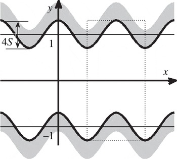
There are an infinite number of possible forms of meandering. This analysis is focused on the simplest case of a channel that follows a sinusoidal path with its geometry specified as (see figure 1)
 $$\begin{eqnarray}\left.\begin{array}{@{}l@{}}y_{U}(x)=1+2S\cos ({\it\alpha}x)=1+(S\text{e}^{\text{i}{\it\alpha}x}+\text{c.c.}),\\ y_{L}(x)=-1+2S\cos ({\it\alpha}x)=-1+(S\text{e}^{\text{i}{\it\alpha}x}+\text{c.c.}),\end{array}\right\}\end{eqnarray}$$
where subscripts
 $U$
and
 $L$
refer to the upper and lower walls, respectively, the amplitude of meandering is
 $2S$
,
 ${\it\lambda}=2{\rm\pi}/{\it\alpha}$
is the wavelength of one cycle of meandering,
 $\text{c.c.}$
stands for the complex conjugate, and half of the mean channel opening
 $h$
is used as the length scale. The channel extends from
 $+\infty$
to
 $-\infty$
in the
 $x$
direction and the flow is driven by a pressure gradient.
Sketch of the flow domain. The dotted line identifies the computational domain for the IBC method.

2.1. Model problem
The flow in a straight channel is described by the velocity
 $\boldsymbol{V}_{0}$
, the pressure
 $p_{0}$
, the stream function
 ${\it\Psi}_{0}$
and the flow rate
 $Q_{0}$
of the form
 $$\begin{eqnarray}\left.\begin{array}{@{}c@{}}\boldsymbol{V}_{0}(\boldsymbol{X})=\left[u_{0}(x,y),v_{0}(x,y)\right]=\left[u_{0}(y),0\right]=\left[1-y^{2},0\right]\!,\\ p_{0}(\boldsymbol{X})=-2x/\mathit{Re},\\ {\it\Psi}_{0}(\boldsymbol{X})=-y^{3}/3+y+2/3,\quad Q_{0}=4/3,\end{array}\right\}\end{eqnarray}$$
where the movement of the fluid is directed towards the positive
 $x$
-axis, the Reynolds number
 $\mathit{Re}$
is defined on the basis of the maximum
 $x$
-velocity and the channel half-height and
 $\boldsymbol{X}=(x\boldsymbol{i}+y\boldsymbol{j}),\boldsymbol{V}_{0}=(u_{0}\boldsymbol{i}+v_{0}\boldsymbol{j})$
. The flow in the meandering channel is represented as
 $$\begin{eqnarray}\left.\begin{array}{@{}c@{}}\boldsymbol{V}_{b}(\boldsymbol{X})=\boldsymbol{V}_{0}(\boldsymbol{X})+\boldsymbol{V}_{1}(\boldsymbol{X})=\left[u_{0}(y),0\right]+\left[u_{1}(x,y),v_{1}(x,y)\right]\!,\\ p_{b}(\boldsymbol{X})=p_{0}(\boldsymbol{X})+p_{1}(\boldsymbol{X}),\quad {\it\Psi}_{b}(\boldsymbol{X})={\it\Psi}_{0}(y)+{\it\Psi}_{1}(x,y),\quad Q_{b}=Q_{0}+Q_{1},\end{array}\right\}\end{eqnarray}$$
where
 $\boldsymbol{V}_{b}=(u_{b}\boldsymbol{i}+v_{b}\boldsymbol{j}),p_{b},{\it\Psi}_{b},Q_{b}$
are the velocity, the pressure, the stream function and the flow rate for the complete flow, respectively, and
 $\boldsymbol{V}_{1},p_{1},{\it\Psi}_{1},Q_{1}$
are the velocity, the pressure, the stream function and the flow rate modifications induced by the channel geometry, respectively. Substitution of (2.3) into the Navier–Stokes and continuity equations and elimination of pressure permit expression of the field equations in the form
 $$\begin{eqnarray}\displaystyle & & \displaystyle u_{0}\partial _{x}{\rm\nabla}^{2}{\it\Psi}_{1}-D^{2}u_{0}\partial _{x}{\it\Psi}_{1}-\mathit{Re}^{-1}{\rm\nabla}^{4}{\it\Psi}_{1}\nonumber\\ \displaystyle & & \displaystyle \quad =-\partial _{y}\left[\partial _{x}\left\{u_{1}u_{1^{\prime }}\right\}+\partial _{y}\left\{u_{1}v_{1}\right\}\right]+\,\partial _{x}\left[\partial _{x}\left\{u_{1}v_{1}\right\}+\partial _{y}\left\{v_{1}v_{1}\right\}\right],\end{eqnarray}$$
where the curly brackets denote the velocity products and
 $D=\text{d}/\text{d}y$
. The boundary conditions have the form
 $$\begin{eqnarray}\displaystyle & u_{0}\left(y_{U}(x)\right)+u_{1}\left(x,y_{U}(x)\right)=0,\quad v_{1}\left(x,y_{U}(x)\right)=0, & \displaystyle\end{eqnarray}$$
 $$\begin{eqnarray}\displaystyle & u_{0}\left(y_{L}(x)\right)+u_{1}\left(x,y_{L}(x)\right)=0,\quad v_{1}\left(x,y_{L}(x)\right)=0. & \displaystyle\end{eqnarray}$$
 $$\begin{eqnarray}{\it\Psi}_{0}\left(y_{L}(x)\right)+{\it\Psi}_{1}\left(x,y_{L}(x)\right)=0.\end{eqnarray}$$
The problem formulation is closed by imposing the fixed mass flow rate constraint, which can be cast as
 $$\begin{eqnarray}{\it\Psi}_{0}\left(y_{U}(x)\right)+{\it\Psi}_{1}\left(x,y_{U}(x)\right)=4/3.\end{eqnarray}$$
This constraint states that the mass flow rates in the straight reference channel and in the meandering channel are the same, i.e.
 $Q_{1}=0$
. The pressure gradient correction required to drive the flow through the meandering channel can be determined by starting with the stream function expressed as a Fourier expansion of the form
 $$\begin{eqnarray}{\it\Psi}_{1}(x,y)=\mathop{\sum }_{n=-\infty }^{n=+\infty }{\it\Phi}^{(n)}(y)\,\text{e}^{\text{i}n{\it\alpha}x},\end{eqnarray}$$
where
 ${\it\Phi}^{(n)}={\it\Phi}^{(-n)^{\ast }}$
are the reality conditions and stars identify the complex conjugate. Substitution of (2.8) into (2.4) and extraction of the modal equation for
 ${\it\Phi}^{(0)}$
lead to
 $$\begin{eqnarray}D^{4}{\it\Phi}^{(0)}+2{\it\alpha}\,\mathit{Re}\,\text{Im}\left(\mathop{\sum }_{k=1}^{k=+\infty }k\,D^{2}({\it\Phi}^{(k)^{\ast }}\,D{\it\Phi}^{(k)})\right)=0,\end{eqnarray}$$
where
 $\text{Im}$
denotes the imaginary part. A single integration of (2.9) gives
 $$\begin{eqnarray}D^{3}{\it\Phi}^{(0)}+2{\it\alpha}\,\mathit{Re}\,\text{Im}\left(\mathop{\sum }_{k=1}^{k=+\infty }k\,D({\it\Phi}^{(k)^{\ast }}\,D{\it\Phi}^{(k)})\right)=A\,\mathit{Re},\end{eqnarray}$$
where
 $A=\partial p_{1}/\partial x|_{mean}$
describes the mean pressure gradient correction; this can be demonstrated by substituting (2.3) and (2.8) into the
 $x$
-momentum equation, extracting from the pressure field mode corresponding to
 $n=0$
and rearranging the resulting expression.
An alternative closing constraint used in this study, the fixed pressure gradient constraint, assumes that the flows in the straight and sinusoidal channels are driven by the same pressure gradient. Change in the flow rate is then used as a measure of additional flow losses associated with the meandering. The constraint (2.7) needs to be replaced with the condition
 $A=0$
and the corresponding flow rate correction
 $Q_{1}$
can be readily evaluated (Floryan Reference Floryan1997).
2.2. Solution method and flow description
A spectrally accurate solution is sought. The main difficulty, which arises due to the need for an efficient handling of a large number of geometric configurations parametrized by (
 $S,{\it\alpha}$
), is overcome by taking advantage of the immersed boundary condition (IBC) method (Szumbarski & Floryan Reference Szumbarski and Floryan1999; Floryan Reference Floryan2002; Husain & Floryan Reference Husain and Floryan2010). This method uses a regular, fixed computational domain suitable for representing the solution in terms of expansions using the global basis functions. The flow domain is ‘submerged’ inside the computational domain (see figure 1), which necessitates the development of special boundary relations that ensure that the flow boundary conditions are enforced. The unknown stream function in (3.3) is represented as the Fourier expansion (3.7) and the velocity components are represented as
 $$\begin{eqnarray}u_{1}(x,y)=\mathop{\sum }_{n=-\infty }^{n=+\infty }u_{1}^{(n)}(y)\,\text{e}^{\text{i}n{\it\alpha}x},\quad v_{1}(x,y)=\mathop{\sum }_{n=-\infty }^{n=+\infty }v_{1}^{(n)}(y)\,\text{e}^{\text{i}n{\it\alpha}x},\end{eqnarray}$$
where
 $u_{1}^{(n)}=u_{1}^{(n)^{\ast }}$
,
 $v_{1}^{(n)}=v_{1}^{(n)^{\ast }}$
are the reality conditions and stars identify the complex conjugate. The modal functions in (2.8) and (2.11) are discretized using the Chebyshev expansions and the Galerkin projection method is used to construct algebraic equations. The boundary constraints are imposed using the tau concept. Details of the algorithm can be found in Floryan (Reference Floryan2002) and Husain & Floryan (Reference Husain and Floryan2010) with the computational performance improved through the use of a specialized solver (Husain & Floryan Reference Husain and Floryan2013). Certain limiting cases have been solved using the domain transformation (DT) method (Husain, Floryan & Szumbarski Reference Husain, Floryan and Szumbarski2009; Mohammadi & Floryan Reference Mohammadi and Floryan2013a
), where the channel is mapped analytically onto a rectangular strip and the field equations are discretized using the Fourier expansions in the streamwise direction and the Chebyshev expansions in the transverse direction. The IBC method is generally much faster computationally but the DT method is more suitable for analysis of limiting cases. Testing of the accuracy of the IBC method is discussed in § 3.1.
A simpler solution can be obtained by considering the limit
 ${\it\alpha}\rightarrow 0$
. The flow domain is regularized using transformation
 ${\it\eta}=y-2S\cos ({\it\xi})$
, where
 ${\it\xi}={\it\alpha}x$
is a slow scale, resulting in the following field equations of the form
 $$\begin{eqnarray}{\it\alpha}\frac{\partial u_{b}}{\partial {\it\xi}}+2S{\it\alpha}\sin ({\it\xi})\frac{\partial u_{b}}{\partial {\it\eta}}+\frac{\partial v_{b}}{\partial {\it\eta}}=0,\end{eqnarray}$$
 $$\begin{eqnarray}\displaystyle & & \displaystyle -\!\left(1+4S^{2}{\it\alpha}^{2}\sin ^{2}({\it\xi})\right)\frac{\partial ^{2}u_{b}}{\partial {\it\eta}^{2}}-{\it\alpha}^{2}\frac{\partial ^{2}u_{b}}{\partial {\it\xi}^{2}}-4S{\it\alpha}^{2}\sin ({\it\xi})\frac{\partial ^{2}u_{b}}{\partial {\it\xi}\partial {\it\eta}}\nonumber\\ \displaystyle & & \displaystyle \qquad -\,2S{\it\alpha}^{2}\cos ({\it\xi})\frac{\partial u_{b}}{\partial {\it\eta}}+2S{\it\alpha}\,\mathit{Re}\,\sin ({\it\xi})\,u_{b}\frac{\partial u_{b}}{\partial {\it\eta}}+\mathit{Re}\,v_{b}\frac{\partial u_{b}}{\partial {\it\eta}}\nonumber\\ \displaystyle & & \displaystyle \qquad +\,{\it\alpha}\,\mathit{Re}\,u_{b}\frac{\partial u_{b}}{\partial {\it\xi}}+{\it\alpha}\,\mathit{Re}\frac{\partial p_{b}}{\partial {\it\xi}}+2S\,{\it\alpha}\,\mathit{Re}\sin ({\it\xi})\frac{\partial p_{b}}{\partial {\it\eta}}=0,\end{eqnarray}$$
 $$\begin{eqnarray}\displaystyle & & \displaystyle -\!\left(1+4S^{2}{\it\alpha}^{2}\sin ^{2}({\it\xi})\right)\frac{\partial ^{2}v_{b}}{\partial {\it\eta}^{2}}-{\it\alpha}^{2}\frac{\partial ^{2}v_{b}}{\partial {\it\xi}^{2}}-4S{\it\alpha}^{2}\sin ({\it\xi})\frac{\partial ^{2}v_{b}}{\partial {\it\xi}\partial {\it\eta}}-2S{\it\alpha}^{2}\cos ({\it\xi})\frac{\partial v_{b}}{\partial {\it\eta}}\nonumber\\ \displaystyle & & \displaystyle \qquad +\,2S{\it\alpha}\,\mathit{Re}\,\sin ({\it\xi})\,u_{b}\frac{\partial v_{b}}{\partial {\it\eta}}+\mathit{Re}\,v_{b}\frac{\partial v_{b}}{\partial {\it\eta}}+{\it\alpha}\,\mathit{Re}\,u_{b}\frac{\partial v_{b}}{\partial {\it\xi}}+\mathit{Re}\frac{\partial p_{b}}{\partial {\it\eta}}=0,\end{eqnarray}$$
 $$\begin{eqnarray}u_{b}=v_{b}=0\quad \text{at}~{\it\eta}=\pm 1,\quad Q_{b}=\int _{-1}^{1}u_{b}({\it\xi},{\it\eta})\text{d}{\it\eta}=\frac{4}{3}.\end{eqnarray}$$
 ${\it\alpha}$
, i.e.
 $$\begin{eqnarray}u_{b}=\hat{u} _{0}+{\it\alpha}^{2}\,\hat{u} _{2}+O({\it\alpha}^{3}),\quad v_{b}={\it\alpha}\,\hat{v}_{1}+O({\it\alpha}^{3}),\quad p_{b}={\it\alpha}^{-1}\hat{p}_{-1}+{\it\alpha}\hat{p}_{1}+O({\it\alpha}^{2}),\end{eqnarray}$$
where
 $$\begin{eqnarray}u_{0}=(1-{\it\eta}^{2}),\quad \hat{u} _{2}=-{\textstyle \frac{4}{3}}S\cos ({\it\xi})\,{\it\eta}\,(1-{\it\eta}^{2}),\end{eqnarray}$$
 $$\begin{eqnarray}v_{1}=-2S\sin ({\it\xi})\,(1-{\it\eta}^{2}),\end{eqnarray}$$
 $$\begin{eqnarray}\hat{p}_{-1}=-2\,\mathit{Re}^{-1}{\it\xi}+\text{const.},\quad \hat{p}_{1}=-4S\,\mathit{Re}^{-1}\left[2S{\it\xi}-{\it\eta}\,\sin ({\it\xi})+S\sin (2{\it\xi})\right],\end{eqnarray}$$
 $$\begin{eqnarray}\displaystyle \frac{\text{d}p_{b}}{\text{d}x}=-2\,\mathit{Re}^{-1}-4{\it\alpha}^{2}\,S\,\mathit{Re}^{-1}\left[2S-y\cos ({\it\alpha}x)\right]+0({\it\alpha}^{3}),\end{eqnarray}$$
 $$\begin{eqnarray}\displaystyle \mathit{Re}\,A=\left.\mathit{Re}\frac{\text{d}p_{1}}{\text{d}x}\right|_{mean}=-8{\it\alpha}^{2}S^{2}.\end{eqnarray}$$
Equation (2.13j
) demonstrates that the pressure losses decrease proportionally to
 ${\it\alpha}^{2}$
when
 ${\it\alpha}\rightarrow 0$
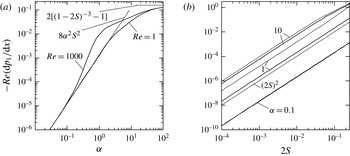
. This decrease is illustrated in figure 2(a). A similar solution can be developed for the fixed pressure gradient case (not shown).
Variations of the pressure gradient correction
 $\mathit{Re}\,(\text{d}p_{1}/\text{d}x)$
, (a) as a function of
 ${\it\alpha}$
for
 $S=0.0125$
and (b) as a function of
 $S$
for
 ${\it\alpha}=0.1$
, 1, 10. In (b), solid and dashed lines correspond to
 $\mathit{Re}=1$
and 1000, respectively.

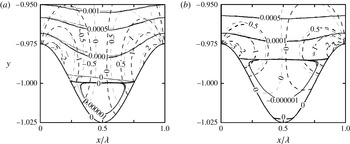
Streamlines (solid lines) and lines of constant pressure
 $\mathit{Re}\,p$
(dashed lines) in the area adjacent to the lower wall for
 $S=0.0125$
,
 $\mathit{Re}=1$
(black lines) and
 $\mathit{Re}=1000$
(grey lines),
 ${\it\alpha}=50$
(a) and
 ${\it\alpha}=100$
(b).

Useful information about the flow properties can be deduced by considering the large wavenumber limit (
 ${\it\alpha}\rightarrow \infty$
). Analysis of flow patterns, such as those shown in figure 3, demonstrates that a reduction of the meandering wavelength results in the formation of separation zones in the troughs. The stream lifts above the ridges and the flow becomes nearly rectilinear, eliminating the centrifugal force field. The flow assumes a form very similar to that in a smooth channel but with both walls shifted inwards by the distance
 $2S$
(Mohammadi & Floryan Reference Mohammadi and Floryan2013a
). It can be shown that the upper bound on the pressure gradient correction is of the form
 $$\begin{eqnarray}\mathit{Re}\,A=2\!\left[1-\left(1-2S\right)^{-3}\right]\!,\end{eqnarray}$$
as verified by the results displayed in figure 2(a). The above expression provides only an upper bound as the actual flow is bounded by ridges with stagnant fluid in between, resulting in a lower shear when compared with shear at the solid wall.
The mechanics of drag formation can be explained by considering the small-amplitude meandering (
 $S\rightarrow 0$
). Such geometries are attractive due to our interest in meandering that creates the minimum pressure loss. It is possible to show that the change in the pressure gradient is generated by the nonlinear effects and it increases proportionally with
 $S^{2}$
for sufficiently small
 $S$
(see appendix A). Such a solution provides a good approximation even for
 $S=0.1$
, as demonstrated by results displayed in figure 2(b).
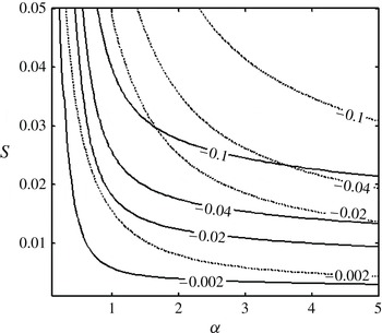
The variations of the pressure losses as a function of
 $S$
and
 ${\it\alpha}$
are illustrated in figure 4. It can be seen that a reduction of the wavelength below
 ${\it\alpha}\approx 2$
leads to a rapid reduction of the required pressure gradient. It will be shown in the next section that such wavelengths are of most interest for the potential applications involving generation of streamwise vortices.
Variations of the pressure gradient correction
 $\mathit{Re}\,(\text{d}p_{1}/\text{d}x)$
as a function of
 $S$
and
 ${\it\alpha}$
for
 $\mathit{Re}=1$
(dashed lines) and
 $\mathit{Re}=1000$
(solid lines).

3. Linear stability analysis of the meandering flow
The conditions leading to the formation of streamwise vortices will be determined using the linear stability theory. The same theory can establish conditions leading to the growth of the travelling wave instability. We begin with the velocity–vorticity form of the governing equations (Floryan Reference Floryan1997), i.e.
 $$\begin{eqnarray}\frac{\partial {\bf\omega}}{\partial t}-({\bf\omega}\boldsymbol{\cdot }\boldsymbol{{\rm\nabla}})\boldsymbol{V}+(\boldsymbol{V}\boldsymbol{\cdot }\boldsymbol{{\rm\nabla}})\,{\bf\omega}={\rm\nabla}^{2}{\bf\omega},\quad \boldsymbol{{\rm\nabla}}\boldsymbol{\cdot }\;\boldsymbol{V}=0,\quad {\bf\omega}=\boldsymbol{{\rm\nabla}}\times \boldsymbol{V},\end{eqnarray}$$
where
 ${\bf\omega}$
and
 $\boldsymbol{V}$
are the vorticity and velocity vectors, respectively. Three-dimensional disturbances are superposed on the base flow in the form
 $$\begin{eqnarray}{\bf\omega}={\bf\omega}_{b}(x,y)+{\bf\omega}_{2}(x,y,z,t),\quad \boldsymbol{V}=\boldsymbol{V}_{b}(x,y)+\boldsymbol{V}_{2}(x,y,z,t),\end{eqnarray}$$
where the subscript
 $b$
refers to the stationary flow discussed in the previous section, subscript 2 refers to the disturbance fields, and
 $\boldsymbol{V}_{2}=(u_{2},v_{2},w_{2})$
and
 ${\bf\omega}_{2}=({\it\omega}_{x2},{\it\omega}_{y2},{\it\omega}_{z2})$
are the disturbance velocity and vorticity vectors. The flow quantities (3.2) are substituted into (3.1), the basic state is subtracted and the equations are linearized. The resulting disturbance equations have the form
 $$\begin{eqnarray}\frac{\partial {\bf\omega}_{2}}{\partial t}+(\boldsymbol{V}_{b}\boldsymbol{\cdot }\boldsymbol{{\rm\nabla}}){\bf\omega}_{2}-({\bf\omega}_{2}\boldsymbol{\cdot }\boldsymbol{{\rm\nabla}})\boldsymbol{V}_{b}+(\boldsymbol{V}_{2}\boldsymbol{\cdot }\boldsymbol{{\rm\nabla}}){\bf\omega}_{b}-({\bf\omega}_{b}\boldsymbol{\cdot }\boldsymbol{{\rm\nabla}})\boldsymbol{V}_{2}=\mathit{Re}^{-1}{\rm\nabla}^{2}{\bf\omega}_{2},\end{eqnarray}$$
 $$\begin{eqnarray}\boldsymbol{{\rm\nabla}}\;\boldsymbol{\cdot }\boldsymbol{V}_{2}=0,\quad {\bf\omega}_{2}=\boldsymbol{{\rm\nabla}}\times \boldsymbol{V}_{2}\end{eqnarray}$$
and are subject to the homogeneous boundary conditions
 $$\begin{eqnarray}\boldsymbol{V}_{2}(x,y_{L},z,t)=0,\quad \boldsymbol{V}_{2}(x,y_{U},z,t)=0\end{eqnarray}$$
at the walls. The disturbance equation (3.3) has coefficients that are functions of
 $x$
and
 $y$
and thus the solution can be written in the form
 $$\begin{eqnarray}\displaystyle & \displaystyle {\bf\omega}_{2}(x,y,z,t)=\tilde{{\bf\omega}}_{2}(x,y)\,\text{e}^{\text{i}({\it\delta}x+{\it\mu}z-{\it\sigma}t)}+\text{c.c.}, & \displaystyle\end{eqnarray}$$
 $$\begin{eqnarray}\displaystyle & \displaystyle \boldsymbol{V}_{2}(x,y,z,t)=\tilde{\boldsymbol{V}}_{2}(x,y)\,\text{e}^{\text{i}({\it\delta}x+{\it\mu}z-{\it\sigma}t)}+\text{c.c.}, & \displaystyle\end{eqnarray}$$
 ${\it\delta}$
and
 ${\it\mu}$
are the real wavenumbers,
 $\tilde{{\bf\omega}}_{2}(x,y)$
and
 $\tilde{\boldsymbol{V}}_{2}(x,y)$
are the
 $x$
-periodic amplitude functions, the real part of the exponent
 ${\it\sigma}={\it\sigma}_{r}+\text{i}{\it\sigma}_{i}$
describes the frequency and its imaginary part describes the growth rate, whilst
 $\text{c.c.}$
stands for the complex conjugate.
The set (
 ${\it\delta},{\it\mu},{\it\sigma}$
) represents the eigenvalues for the specified flow conditions (
 $\mathit{Re},S,{\it\alpha}$
) creating a very large parameter space. To derive the eigenvalue problem for the partial differential equations (3.3) in a form that is suitable for efficient computations, we take advantage of the periodicity of the amplitude functions and represent them in terms of Fourier expansions of the form
 $$\begin{eqnarray}\displaystyle & \displaystyle \tilde{{\bf\omega}}_{2}(x,y)=\text{i}\mathop{\sum }_{m=-\infty }^{m=+\infty }\left[{\it\zeta}_{x}^{(m)}(y),{\it\zeta}_{y}^{(m)}(y),~{\it\zeta}_{z}^{(m)}(y)\right]\,\text{e}^{\text{i}m{\it\alpha}x}, & \displaystyle\end{eqnarray}$$
 $$\begin{eqnarray}\displaystyle & \displaystyle \tilde{\boldsymbol{V}}_{2}(x,y)=\mathop{\sum }_{m=-\infty }^{m=+\infty }\left[g_{u}^{(m)}(y),~g_{v}^{(m)}(y),\,g_{w}^{(m)}(y)\right]\,\text{e}^{\text{i}m{\it\alpha}x}, & \displaystyle\end{eqnarray}$$
 $$\begin{eqnarray}\displaystyle & \displaystyle {\bf\omega}_{2}(x,y,z,t)=\text{i}\mathop{\sum }_{m=-\infty }^{m=+\infty }\left[\,{\it\zeta}_{x}^{(m)}(y),\quad {\it\zeta}_{y}^{(m)}(y),\,\,{\it\zeta}_{z}^{(m)}(y)\right]\,\text{e}^{\text{i}\left[\left({\it\delta}+m{\it\alpha}\right)x+{\it\mu}z-{\it\sigma}t\right]}+\text{c.c.}, & \displaystyle\end{eqnarray}$$
 $$\begin{eqnarray}\displaystyle & \displaystyle \boldsymbol{V}_{2}(x,y,z,t)=\mathop{\sum }_{m=-\infty }^{m=+\infty }\left[g_{u}^{(m)}(y),\,g_{v}^{(m)}(y),\,g_{w}^{(m)}(y)\right]\,\text{e}^{\text{i}\left[\left({\it\delta}+m{\it\alpha}\right)x+{\it\mu}z-{\it\sigma}t\right]}+\text{c.c.} & \displaystyle\end{eqnarray}$$
 $$\begin{eqnarray}\displaystyle & \displaystyle A^{(m)}{\it\zeta}_{y}^{(m)}+Bg_{v}^{(m)}=\mathit{Re}\,\mathop{\sum }_{n=-\infty }^{n=+\infty }\left(H_{{\it\zeta}}^{(m-n)}{\it\zeta}_{y}^{(m-n)}+H_{v}^{(m-n)}g_{v}^{(m-n)}\right)\!, & \displaystyle\end{eqnarray}$$
 $$\begin{eqnarray}\displaystyle & \displaystyle C^{(m)}g_{v}^{(m)}=-\mathit{Re}\,\mathop{\sum }_{n=-\infty }^{n=+\infty }\left(I_{{\it\zeta}}^{(m-n)}{\it\zeta}_{y}^{(m-n)}+I_{v}^{(m-n)}g_{v}^{(m-n)}\right) & \displaystyle\end{eqnarray}$$
 $-\infty <m<+\infty$
subject to boundary conditions (3.3d,e
). In the above,
 $$\begin{eqnarray}A^{(m)}=D^{2}-k_{m}^{2}-\text{i}\,\mathit{Re}\,1(t_{m}u_{0}-{\it\sigma}),\quad B=\mathit{Re}\,{\it\mu}Du_{0},\end{eqnarray}$$
 $$\begin{eqnarray}C^{(m)}=(D^{2}-k_{m}^{2})^{2}-\text{i}\,\mathit{Re}[(t_{m}u_{0}-{\it\sigma})(D^{2}-k_{m}^{2})-t_{m}D^{2}u_{0}],\end{eqnarray}$$
 $$\begin{eqnarray}t_{m}=m{\it\alpha}+{\it\delta},\quad k_{m}^{2}=t_{m}^{2}+{\it\mu}^{2},\end{eqnarray}$$
 $$\begin{eqnarray}H_{{\it\zeta}}^{(m-n)}=\text{i}t_{m}u_{1}^{(n)}+k_{m-n}^{-2}({\it\mu}^{2}+t_{m-n}t_{m})\,v_{1}^{(n)}D,\end{eqnarray}$$
 $$\begin{eqnarray}H_{v}^{(m-n)}=-{\it\mu}\,Du_{1}^{(n)}+\text{i}n\,{\it\alpha}{\it\mu}\,k_{m-n}^{-2}\,v_{1}^{(n)}\,D^{2},\end{eqnarray}$$
 $$\begin{eqnarray}I_{{\it\zeta}}^{(m-n)}=n\,{\it\alpha}\,{\it\mu}\,k_{m-n}^{-2}\left[2t_{m-n}u_{1}^{(n)}D+\left(t_{m}+t_{m-n}\right)\,Du_{1}^{(n)}-\text{i}\,k_{m}^{2}v_{1}^{(n)}-\text{i}\,v_{1}^{(n)}D^{2}\right]\!,\end{eqnarray}$$
 $$\begin{eqnarray}\displaystyle I_{v}^{(m-n)} & = & \displaystyle k_{m-n}^{-2}\left[\text{i}\,n\,{\it\alpha}\,({\it\mu}^{2}-t_{m}t_{m-n})\,Du_{1}^{(n)}D+k_{m}^{2}({\it\mu}^{2}+t_{m-n}t_{m-2n})\,v_{1}^{(n)}D\right.\nonumber\\ \displaystyle & & \displaystyle +\left.\text{i}\,(-k_{m-n}^{2}t_{m}+2n{\it\alpha}{\it\mu})\,\,u_{1}^{(n)}\,D^{2}+(n{\it\alpha}\,t_{m}-k_{m}^{2})\,v_{1}^{(n)}\,D^{3}\right]\nonumber\\ \displaystyle & & \displaystyle +\,\text{i}k_{m}^{2}t_{m-2n}u_{1}^{(n)}+\text{i}t_{m}D^{2}u_{1}^{(n)}.\end{eqnarray}$$
The above formulation uses Bloch theory (Bloch Reference Bloch1928) for systems with spatially periodic coefficients. It is analogous to Floquet theory (Coddington & Levinson Reference Coddington and Levinson1965) for systems with time-periodic coefficients. The eigenvalues of the resulting system have to be determined numerically.
3.1. Numerical solution
Solution of the complete system requires numerical determination of the eigenvalues of (3.3d,e
) and (3.7). Approximate solutions can be found by truncating the sum in (3.6) after a finite number
 $N_{M}$
of terms and solving the eigenvalue problem for
 $2N_{M}+1$
differential equations of type (3.7). The differential equations are discretized with spectral accuracy using Chebyshev expansions and the Galerkin projection method. The boundary conditions at the upper and lower walls are converted into the boundary relations using the IBC concept (Floryan Reference Floryan2002). The discretization procedure results in a matrix eigenvalue problem
 ${\it\bf\Theta}{\it\Lambda}=0$
, where
 ${\it\bf\Theta}({\it\sigma})$
represents the coefficient matrix. This matrix is linear in
 ${\it\sigma}$
, i.e.
 ${\it\bf\Theta}={\it\bf\Theta}_{0}+{\it\bf\Theta}_{1}{\it\sigma}$
, where
 ${\it\bf\Theta}_{0}={\it\bf\Theta}(0)$
,
 ${\it\bf\Theta}_{1}={\it\bf\Theta}(1)-{\it\bf\Theta}_{0}$
. The
 ${\it\sigma}$
-spectrum is determined by solving a general eigenvalue problem in the form
 ${\it\bf\Theta}_{0}{\it\Lambda}={\it\sigma}{\it\bf\Theta}_{1}{\it\Lambda}$
. Several methods for tracing individual eigenvalues have been used, i.e. the shooting method combined with the Newton–Raphson procedure (Floryan Reference Floryan2002), the inverse iteration method (Floryan Reference Floryan2002) and Arnoldi’s method (Saad Reference Saad2003). The tracing of eigenvalues has been extended, if required, over several Brillouin zones (Bloch Reference Bloch1928) in the
 ${\it\delta}$
-direction in order to demonstrate how the leading eigenvalue is affected by the meandering wavelength.
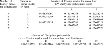
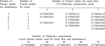
The accuracy of the discretization depends on the number of Chebyshev polynomials and Fourier modes used in the solution for the mean flow, the number of Chebyshev polynomials and Fourier modes used in the solution of the disturbance equations, and the number of Fourier modes used to represent the mean flow in the numerical solution of the disturbance equations. Selection of proper numerical parameters has been done on the basis of convergence tests illustrated in tables 1 and 2 in appendix B.
3.2. Onset of vortices
Channel meandering forces changes in the stream direction and this generates a centrifugal force field which, under certain conditions, may generate instability leading to the formation of streamwise vortices. Such vortices correspond to
 ${\it\delta}=0$
and
 ${\it\sigma}_{r}=0$
in (3.4). The meandering is essential for the formation of the vortices as it can be demonstrated analytically that in its absence (
 $S\rightarrow 0$
) the vortices are attenuated (appendix C). The formation of the vortices is of practical importance as they drastically increase the heat transfer (Jacobi & Shah Reference Jacobi and Shah1995). These vortices add transverse fluid movement, thereby taking heated fluid elements away from the hot wall and bringing cold elements into direct contact with this wall.
The centrifugal instability occurs for a sufficiently high
 $\mathit{Re}$
but only if the form of the meandering satisfies certain conditions. Reduction of
 $\mathit{Re}$
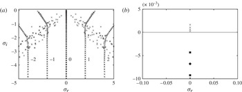
increases viscous dissipation and stabilizes the flow regardless of the type of meandering. The typical spectrum shown in figure 5 demonstrates the existence of many unstable modes. The vertical ‘columns’ of eigenvalues are associated with Fourier modes used in the numerical solution with the number of ‘columns’ equal to the number of Fourier modes. Four eigenvalues are unstable for
 $\mathit{Re}$
used in this test. Tracing of the first two down to
 $S\rightarrow 0$
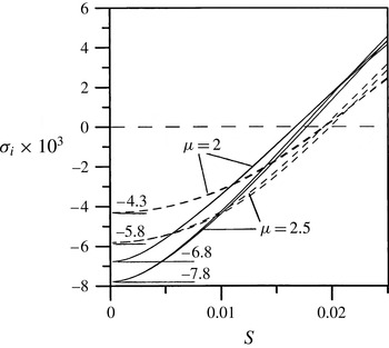
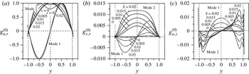
demonstrates that the first (most unstable) eigenvalue connects with the Tollmien–Schlichting spectrum of the smooth channel and the second eigenvalue connects with the Squire spectrum (figure 6). In the straight channel the Squire modes are less attenuated than the TS modes, but the introduction of meandering promotes amplification of the TS mode, and it is this mode, not the Squire mode, that determines the critical conditions. Evolution of the eigenfunctions
 $g_{u}^{(0)},g_{v}^{(0)},g_{w}^{(0)}$
for the two most unstable modes as a function of
 $S$
is illustrated in figure 7.
Spectrum of
 ${\it\sigma}$
for the vortex mode for
 $\mathit{Re}=1500$
,
 $S=0.02$
,
 ${\it\mu}=2$
,
 ${\it\alpha}=3$
and the fixed flow rate constraint: (a) complete spectrum; (b) enlargement focused on the main segment. Numerical symbols in (a) identify elements of the spectrum that correspond to different Fourier modes in (3.6) in the limit of
 $S\rightarrow 0$
. The dots correspond to the Orr–Sommerfeld spectrum and the squares identify the Squire spectrum.

Variations of the amplification rate
 ${\it\sigma}_{i}$
as a function of
 $S$
for vortices with
 ${\it\mu}=2$
,
 ${\it\mu}=2.5$
for
 ${\it\alpha}=3$
,
 $\mathit{Re}=1500$
and the fixed flow rate constraint. Solid and dashed lines correspond to the first and second instability modes, respectively. See appendix C for a discussion of the limit
 $S\rightarrow 0$
.

Evolution of the eigenfunctions
 $g_{u,r}^{(0)}$
(a),
 $g_{v,r}^{(0)}$
(b),
 $g_{w,i}^{(0)}$
(c), normalized with
 $\max (g_{u}^{(0)})=1$
corresponding to the first and second vortex instability modes as a function of
 $S$
for
 ${\it\alpha}=3$
,
 ${\it\mu}=2$
,
 $\mathit{Re}=1500$
and the fixed flow rate constraint.

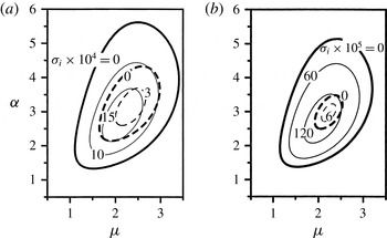
The top eigenvalue from figure 5 has been traced in the (
 ${\it\alpha},{\it\mu}$
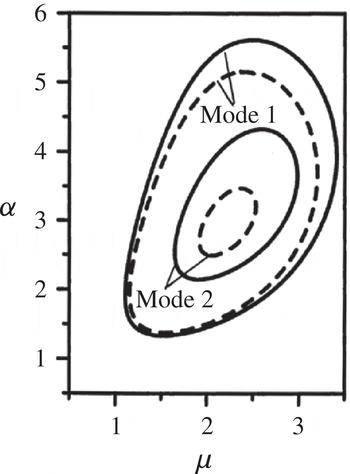
) space illustrating variations of the amplification rate of the most unstable mode. Results displayed in figure 8(a) demonstrate that meanderings that are either too ‘shallow’ (
 ${\it\alpha}\lesssim 1.5$
) or too ‘deep’ (
 ${\it\alpha}\gtrsim 5.6$
) do not produce instability. In the former case the flow turning is insufficient to generate a centrifugal force strong enough to create vortices, while in the latter case the stream lifts up above the ridges, which also reduces the turning effect and thus reduces the centrifugal force. The amplified wavelengths are contained in a finite interval of
 ${\it\mu}$
whose length and location are functions of
 ${\it\alpha}$
. The second mode is more stable in the sense that the range of active
 ${\it\alpha}$
is smaller, the band of the resulting vortices is narrower, and the amplification rates are smaller in comparison to the first mode (figure 8
a).
Variations of the amplification rate
 ${\it\sigma}_{i}$
as a function of
 ${\it\mu}$
and
 ${\it\alpha}$
for vortices for
 $\mathit{Re}=1500$
,
 $S=0.02$
and (a) the fixed flow rate constraint and (b) the fixed pressure gradient constraint. Solid and dashed lines correspond to the first and second instability modes, respectively.

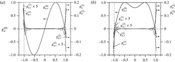
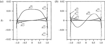
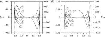
Figures 9–11 illustrate the first three eigenfunctions for disturbance velocity components for the two most unstable instability modes. The dominant character of
 $\text{Re}(g_{u}^{(0)})$
, which is the characteristic feature of the velocity field associated with the vortices (Floryan Reference Floryan1991), is clearly visible (see figure 9). The shape of
 $\text{Re}(g_{v}^{(0)})$
for the first mode (figure 10
a) suggests the existence of a single layer of vortices in the middle of the channel and two layers in the case of the second mode (figure 10
b). The same conclusion can be drawn from distributions of
 $\text{Im}(g_{w}^{(0)})$
displayed in figure 11.
Eigenfunctions
 $g_{u}^{(m)}=g_{u,r}^{(m)}+\text{i}\,g_{u,i}^{(m)}$
for the vortex mode for
 $m=1$
, 2, 3 normalized with condition
 $\max (g_{u}^{(0)})=1$
for
 ${\it\mu}=2$
,
 ${\it\alpha}=3$
,
 $S=0.02$
,
 $\mathit{Re}=1500$
and the fixed flow rate constraint. (a) The first and (b) the second mode of instability.

Eigenfunctions
 $g_{v}^{(m)}=g_{v,r}^{(m)}+\text{i}\,g_{v,i}^{(m)}$
. The remaining conditions are the same as in figure 9.

Eigenfunctions
 $g_{w}^{(m)}=g_{w,r}^{(m)}+\text{i}\,g_{w,i}^{(m)}$
. The remaining conditions are the same as in figure 9.

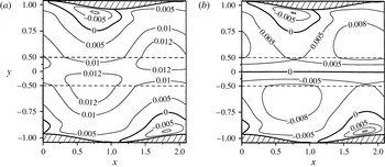
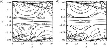
The two modes give rise to very different flow topologies. These topologies are quite complex, and are illustrated in figures 12 and 13 using the velocity ‘amplitude function’
 $\tilde{\boldsymbol{V}}_{2}(x,y)$
(see (3.4)) which, in the case of vortices, can be represented as
 $\tilde{\boldsymbol{V}}_{2}(x,y)=[h_{u}(x,y),\,h_{v}(x,y),\,\,\text{i}\,h_{w}(x,y)]$
, where
 $h_{u},h_{v},h_{w}$
are real. A change of sign of
 $h_{v}$
provides the most reliable criterion for identification of borders between different layers of vortices. Most of the channel is ‘filled in’ with a single layer of vortices associated with the first mode. As the flow meanders and keeps turning up and down, additional layers form in the zones adjacent to the walls that behave as obstacles to the oncoming flow (outer walls with respect to the direction of turning; see figure 12
a). The centrifugal effect is strongest in these locations, where it creates small vortices attached to each wall. The ‘wall’ vortices rotate in the same direction, alternate between the upper and lower walls and are spaced apart by half of the meandering wavelength. These vortices are the primary vortices driven directly by the centrifugal forces, while the large central vortex plays a secondary role. The centrifugal effect is not active along the wall segments that are inner with respect to the direction of turning; the primary vortices do not exist there but the secondary vortex persists due to fluid inertia. As a result, when the fluid moves in the downstream direction, the vortex motion in the central section of the channel receives a periodic boost from the primary vortices. The overall stability depends on whether this boost is strong enough to maintain the vortex motion in the area where the driving force is absent. This situation is qualitatively similar to the instability in the converging–diverging channel, where the primary vortices are located in the converging section and are able to drive the global, secondary vortices that persist through the diverging section (Floryan Reference Floryan2003). A similar situation is likely to occur in many other geometric configurations as long as the local primary vortices are sufficiently strong to maintain the global vortex system. Prediction of the critical conditions, however, cannot be generalized as they depend on the details of the geometry and therefore have to be analysed on a case-by-case basis.
Contour plots of
 $h_{v}(x,y)$
(
 $y$
-component of the velocity ‘amplitude function’
 $\tilde{\boldsymbol{V}}_{2}(x,y)$
; see (3.4)) for (a) the first and (b) the second instability modes. The remaining conditions are the same as in figure 9. Different layers of vortices are identified by changes of sign of
 $h_{v}$
.


The flow topology associated with the second mode is qualitatively similar to the first mode, as illustrated in figures 12 and 13. The primary vortices are attached to the same sections of the walls and are almost identical to those found in the case of the first mode. These ‘wall’ vortices drive two secondary vortices in the central section of the channel. The ‘wall’ vortices rotate in opposite directions in order to maintain kinematic consistency with those in the middle of the channel. Comparison of figures 12(a,b) and 13(a,b) shows that the first mode is symmetric with respect to the channel axis, while the second is asymmetric. It needs to be stressed that the primary ‘wall’ vortices appear to be similar for both modes, with the distinction between these modes being associated with the form of the secondary, central vortices.
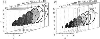
The neutral surfaces in the (
 ${\it\alpha},{\it\mu},S$
) space for the first and second vortex instability modes for (a)
 $\mathit{Re}=1500$
and (b)
 $\mathit{Re}=5000$
and the fixed flow rate constraint.

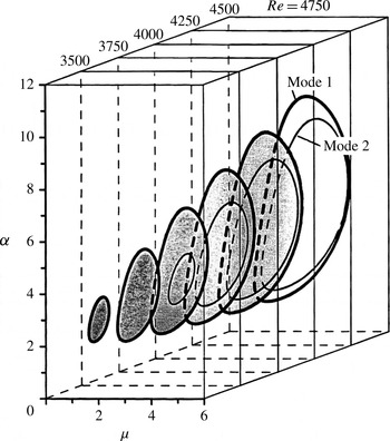
The neutral surfaces in the (
 ${\it\alpha},{\it\mu},Re$
) space for the first and second vortex instability modes for
 $S=0.008$
and the fixed flow rate constraint. The tips of the neutral surfaces define the global critical conditions (
 $\mathit{Re}_{g,cr},{\it\alpha}_{g,cr},{\it\mu}_{g,cr}$
).

Figure 14(a) displays the neutral surfaces in the (
 ${\it\alpha},{\it\mu},S$
) space for
 $\mathit{Re}=1500$
for the first two modes. The first mode is always more unstable, as expected, although the second mode can be induced with a correct combination of initial conditions. There is a range of parameters where only the first mode becomes unstable. The shapes of the neutral surfaces demonstrate that the range of
 ${\it\alpha}$
leading to the instability, as well as the range of the resulting unstable
 ${\it\mu}$
, increase rapidly as the meandering becomes more extreme. Similar results for
 $\mathit{Re}=5000$
displayed in figure 14(b) demonstrate that this increase is more rapid for higher
 $\mathit{Re}$
, where it results in a much wider range of destabilizing
 ${\it\alpha}$
and resulting
 ${\it\mu}$
. It can also be seen that the instability occurs at much smaller
 $S$
when
 $\mathit{Re}$
is higher. Figure 15 displays the neutral surfaces in the (
 ${\it\alpha},{\it\mu},\mathit{Re}$
) space for
 $S=0.008$
. A rapid increase of the range of destabilizing
 ${\it\alpha}$
and the resulting
 ${\it\mu}$
as
 $\mathit{Re}$
increases is clearly visible. Meandering with wavenumbers
 ${\it\alpha}<2$
is of particular interest as it provide an opportunity for the generation of vortices with smaller pressure losses.
The vortices play a dual role in the intensification of the heat transfer. Their appearance results in transverse fluid movement, which directly increases the heat flow. In this case the flow field consists of the reference flow with superposed vortices and the corresponding bifurcation branches are stable. The vortices may also affect the heat transfer indirectly, as they lead to a rapid three-dimensionalization of the flow field; the uplifting of the low momentum fluid away from the wall leads to the formation of highly distorted streamwise and spanwise velocity profiles which are potentially subject to very strong secondary instabilities very similar to those studied in detail in the case of Görtler instability (Floryan Reference Floryan1991). In this case the bifurcating branches correspond to unstable solutions and the onset of the vortices represents just the first step of the by-pass transition to turbulence. The analysis presented in this paper does not address the question of stability of the bifurcating branches. The reader may note that both types of response are possible as one may identify meandering characteristics resulting in a wide range of
 $\mathit{Re}_{cr}$
, including those which lead to relatively small
 $\mathit{Re}_{cr}$
. Very accurate simulations in cases where these branches are unstable document complex saturation states whose structure strongly depends on the details of the channel geometry (Guzmán et al.
Reference Guzmán, Cárdenas, Urzúa and Araya2009; Sui et al.
Reference Sui, Teo and Lee2012). Regardless of whether one is interested in the use of vortices to promote transition or just to provide transverse advection, one would search for the least extreme meandering that leads to the onset of the instability, as this would initiate secondary effects at the lowest cost in terms of pressure loss. For presentation of the results it is convenient to introduce the global critical Reynolds number
 $\mathit{Re}_{g,cr}$
, which defines the critical conditions for the onset of the instability for a given meandering amplitude
 $S$
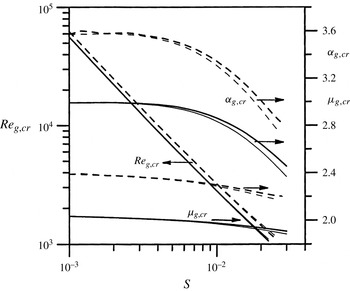
, regardless of its wavelength, as it summarizes the minimal conditions required for the creation of the vortices. Such global critical conditions correspond to the tip of the neutral surface shown in figure 15. Variations of
 $\mathit{Re}_{g,cr,}\,{\it\alpha}_{g,cr}$
,
 ${\it\mu}_{g,cr}$
as a function of
 $S$
are illustrated in figure 16 for both modes. The area below the critical curves defines the range of
 $S$
and
 $\mathit{Re}$
for which the flow is stable. The first mode determines the critical stability conditions, although the second mode can be induced with a correct selection of the initial conditions if
 $\mathit{Re}$
is high enough. It is worth noting that
 ${\it\alpha}_{g,cr}$
for the second mode is about 30 % larger than for the first mode, while
 ${\it\mu}_{g,cr}$
is about 20 % larger.
Variations of the global critical stability conditions
 $\mathit{Re}_{g,cr}$
,
 ${\it\alpha}_{g,cr}$
,
 ${\it\mu}_{g,cr}$
for the vortex mode as a function of
 $S$
. The solid and dashed lines correspond to the first and second instability modes, respectively. The thick and thin lines correspond to the flow with the fixed flow rate and the fixed pressure gradient constraints, respectively.

The results presented so far have dealt with the stability of a flow that is developed under the fixed flow rate constraint. As the amplitude of meandering increases, the pressure gradient needs to be increased in order to support such a flow (§ 2). If the pressure gradient remains constant, the flow should slow down, resulting in reduction of the mass flow rate, reduction of the centrifugal effect and flow stabilization. Figure 5 displays the amplification rates for the two most unstable modes for both types of constraints. Their comparison demonstrates the relative flow stabilization associated with the fixed pressure gradient constraint. Comparison of the neutral curves for both types of flow, displayed in figure 17, underlines this stabilization and provides its quantitative measure. The onset of the instability, as measured by
 $\mathit{Re}_{g,cr}$
, takes place under almost the same conditions for both types of flow, as shown in figure 16. The small difference of
 $\mathit{Re}_{g,cr}$
increases with an increase of
 $S$
, with the flow with the fixed pressure gradient always being more stable. The increase of this difference is due to the progressively higher flow resistance associated with larger
 $S$
(see § 2).
Neutral curves describing the first two modes of the vortex instability in a flow subject to the fixed flow rate constraint (solid lines) and to the fixed pressure gradient constraint (dashed lines). The remaining conditions are the same as in figure 8.

3.3. Travelling wave mode
Creation of the vortices through the centrifugal instability mechanism can be affected by the shear-driven instabilities which, once established, could prevent formation of the vortices. It is well known that flow in a straight channel is subject to the shear-driven, travelling (Tollmien–Schlichting or TS) wave instability when the
 $\mathit{Re}$
reaches the critical value of
 $\mathit{Re}_{cr}=5772$
. The critical wave has a two-dimensional form characterized by the wavevector
 $({\it\delta}_{cr},{\it\mu}_{cr})=(1.02,0)$
and propagates in the downstream direction. The bifurcation has a subcritical character, and an increase in the level of background disturbances can reduce the critical Reynolds number down to
 $\mathit{Re}_{cr}\approx 2700$
(Herbert Reference Herbert1988).
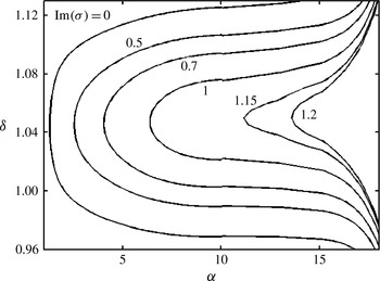
A typical spectrum shown in figure 18 for a two-dimensional TS wave with
 $({\it\delta},{\it\mu})=(1.04,0)$
for
 $S=0.005$
,
 ${\it\alpha}=1$
,
 $\mathit{Re}=6000$
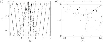
and the fixed mass constraint shows the existence of only one unstable eigenvalue. The spectrum consists of vertical ‘columns’, associated with different Fourier modes present in (3.5), with each segment consisting of the
 $A$
,
 $P$
and
 $S$
branches, similar to the case of the Orr–Sommerfeld operator (Mack Reference Mack1976). The Orr–Sommerfeld spectrum for the same disturbance in a straight channel is shown for comparison purposes. The complete spectrum looks like a superposition of spectra for a set of TS waves with the wavenumbers
 ${\it\delta}=1.04\pm 2~\text{m}$
, with the dominant wave corresponding to
 $m=0$
in (3.5), and indeed, in the limit of
 $S=0$
this spectrum separates into independent segments associated with such TS waves.
Spectrum of
 ${\it\sigma}$
for the TS wave with the wavevector
 $({\it\delta},{\it\mu})=(1.04,0)$
for
 $S=0.005$
,
 ${\it\alpha}=1$
,
 $\mathit{Re}=6000$
and the fixed flow rate constraint: (a) complete spectrum; (b) enlargement focused on the main segment. Numerical symbols in (a) identify elements of the spectrum that correspond to different Fourier modes in (3.6) in the limit of
 $S\rightarrow 0$
. The
 $A$
,
 $P$
and
 $S$
branches of the main Fourier mode (corresponding to
 $m=0$
in (3.6) for
 $S\rightarrow 0$
) are identified using the symbols
 $A,P,S$
, respectively. The dots correspond to the Orr–Sommerfeld spectrum.

Variations of the amplification rate
 ${\it\sigma}_{i}$
as a function of
 ${\it\delta}$
for
 $S=0.005$
,
 ${\it\alpha}=1$
,
 $\mathit{Re}=6000$
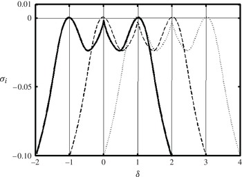
and the fixed flow rate constraint. The maximum amplification for these conditions corresponds to
 ${\it\delta}=1.04$
. Solid, dashed and dotted lines identify three families of solutions corresponding to
 ${\it\delta}$
,
 ${\it\delta}+{\it\alpha}$
,
 ${\it\delta}+2{\it\alpha}$
. Vertical lines mark boundaries between Brillouin zones. Results of tracing for the TS wave in a smooth channel overlap with the solid line within the resolution of this figure.

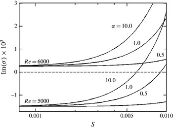
Variations of the amplification rate
 ${\it\sigma}_{i}$
for the two-dimensional TS wave with
 ${\it\delta}=1.04$
as a function of
 $S$
for the fixed flow rate constraint.

Tracing of the unstable eigenvalue shown in figure 18 as a function of
 $\mathit{Re}$
,
 ${\it\delta}$
,
 ${\it\alpha}$
,
 $S$
provides information about the flow stability characteristics. One type of tracing, i.e. tracing of
 ${\it\sigma}$
as a function of
 ${\it\delta}$
, leads to interpretation difficulties as solutions of type (3.6) are identical for
 ${\it\delta}=m{\it\alpha}$
. The
 ${\it\delta}$
-axis can be divided into an infinite set of Brillouin zones with ends located at
 ${\it\delta}=\pm m{\it\alpha}$
, with identical variations of
 ${\it\sigma}_{i}$
in each zone. Values of
 ${\it\delta}$
that are of physical interest may extend over several Brillouin zones, and therefore one has to identify proper connections between different branches in each Brillouin zone in order to construct a continuous and physically relevant relation
 ${\it\sigma}_{i}({\it\delta})$
extending over the range of
 ${\it\delta}$
of physical interest. There are multiple relations with the property
 ${\it\sigma}_{i}({\it\delta})={\it\sigma}_{i}({\it\delta}+m{\it\alpha})$
, which makes some of the eigenvalues in the spectrum shown in figure 18 physically irrelevant as they belong to curve
 ${\it\sigma}_{i}({\it\delta})$
shifted by
 $n{\it\alpha}$
in the
 ${\it\delta}$
-direction. Several of the top eigenvalues in this spectrum correspond to branches associated with modes
 $\pm m$
, each of which has a similar periodicity in the
 ${\it\delta}$
-direction, and this adds to the interpretation difficulties. Variations of the physically relevant eigenvalues as a function of
 ${\it\delta}$
can nevertheless be traced, with the inverse iteration being the most reliable tracing method. The reliability of the tracing was verified by studying modal shapes and by taking the limit of
 $S\rightarrow 0$
to make sure that the correct mode was followed. The results of the tracing process are illustrated in figure 19.
Variations of the amplification rate
 ${\it\sigma}_{i}$
of the two-dimensional TS waves as a function of
 ${\it\alpha}$
and
 ${\it\delta}$
for
 $S=0.008$
,
 $\mathit{Re}=5000$
and the fixed flow rate constraint.

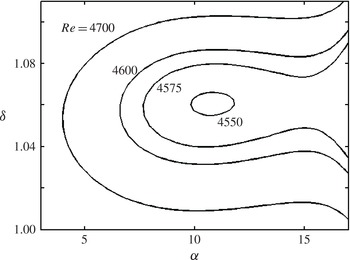
The neutral stability curves for the two-dimensional TS waves as a function of
 ${\it\delta}$
and
 ${\it\alpha}$
for (a)
 $\mathit{Re}=5000$
and (b)
 $\mathit{Re}=6000$
for the fixed flow rate constraint.

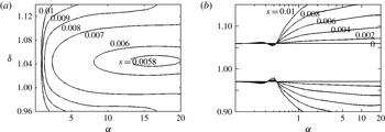
The results displayed in figure 20 demonstrate that meandering destabilizes TS waves, with its effectiveness rapidly increasing with
 $S$
. Figure 21 illustrates variations of the amplification rates as a function of
 ${\it\alpha}$
for a fixed
 $S$
and a subcritical
 $\mathit{Re}=5000$
, and demonstrates that an increase of
 ${\it\alpha}$
causes more pronounced destabilization. Use of large
 ${\it\alpha}$
results in an effective narrowing of the channel opening (see § 2.2), with the flow lifting above the ridges and becoming nearly rectilinear (see figure 3). The flow accelerates as the same mass flow has to pass through a narrower channel, but
 $\mathit{Re}$
remains the same due to the fixed flow rate constraint. The destabilization is associated with the change of the character of the wall layers but details of the mechanics of the flow response remain to be delineated. This particular limit is of no interest in the current analysis as the meandering effect is either reduced or eliminated under such conditions. Figure 22(a) displays the neutral stability curves for the same subcritical
 $\mathit{Re}=5000$
but for different amplitudes of meandering. Reduction of
 $S$
shifts the unstable region towards larger
 ${\it\alpha}$
and eventually leads to the complete stabilization of TS waves. Figure 22(b) displays the neutral stability curves for the supercritical
 $\mathit{Re}=6000$
. One can see expansion of the range of unstable
 ${\it\delta}$
with an increase of
 $S$
, with this expansion being more pronounced for larger
 ${\it\alpha}$
. Figure 23 displays variations of the neutral stability curves due to changes of
 $\mathit{Re}$
. As expected, a sufficient reduction of
 $\mathit{Re}$
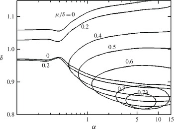
stabilizes the TS waves. Figure 24 displays the neutral curves for the oblique waves and demonstrates that the two-dimensional waves retain their critical role in the meandering channel.
The neutral stability curves for the two-dimensional TS waves as a function of
 ${\it\delta}$
and
 ${\it\alpha}$
for
 $S=0.008$
and the fixed flow rate constraint.

The neutral stability curves for the oblique TS waves as a function of
 ${\it\delta}$
and
 ${\it\alpha}$
for
 $S=0.008$
,
 $\mathit{Re}=6000$
and the fixed flow rate constraint.

3.4. Competition between the travelling wave mode and the vortex mode
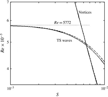
The presence of two instability mechanisms raises the question of when each of them will dominate the instability process. Figure 25 presents variations of the global critical
 $\mathit{Re}_{g,cr}$
as a function of
 $S$
for both types of instability. The reader may recall that
 $\mathit{Re}_{g,cr}$
corresponds to the minimum of
 $\mathit{Re}_{cr}$
over all
 ${\it\alpha}$
for a fixed S. The global critical curves cross each other at
 $(S,\mathit{Re}_{g,cr})=(0.00642,4870)$
for the fixed flow rate constraint and (0.00638, 4935) for the fixed pressure gradient constraint. The crossing points correspond in the case of TS waves to
 ${\it\alpha}=14.6$
(fixed flow rate) and
 ${\it\alpha}=13.3$
(fixed pressure gradient) and to
 ${\it\alpha}=2.95$
for vortices for both types of constraint.
Variations of the global critical Reynolds number
 $\mathit{Re}_{g,cr}$
for the vortex and TS wave modes as functions of
 $S$
. The solid and dashed lines correspond to the fixed flow rate and the fixed pressure gradient constraints, respectively.

(a) Variations in the critical Reynolds number
 $\mathit{Re}_{cr}$
for the onset of the vortex (solid lines) and the TS wave (dashed lines) instabilities, and (b) the pressure gradient correction corresponding to the onset of the vortex instability, as functions of
 $S$
and
 ${\it\alpha}$
. The parameter range indicated by the thick line identifies geometries where the vortex mode plays a critical role.

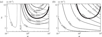
A closer look at the competition between the two modes is provided by the data displayed in figure 26(a). It can be seen that
 $\mathit{Re}_{cr}$
decreases with an increase of
 $S$
for both modes; this decrease is more rapid for the vortices than for the TS waves but only as long as the meandering wavelength is neither too short nor too long.
 $S$
needs to reach a minimum of about
 $S=0.006$
for
 $\mathit{Re}_{cr}$
for the two modes to become equal (at
 $\mathit{Re}_{cr}\approx 5300$
) and this occurs for
 ${\it\alpha}\approx 2.5$
. Further increase of
 $S$
builds up the advantage for the vortices. At
 $S=0.0125$
,
 $\mathit{Ra}_{cr}$
for the vortices is reduced to
 $\mathit{Re}_{cr}\approx 2000$
but
 $\mathit{Ra}_{cr}$
for the TS waves is reduced to only
 $\mathit{Re}_{cr}\approx 4000$
. It is therefore possible to select a meandering geometry that will lead to the formation of the vortices without interference from the TS waves. The large difference between
 $\mathit{Re}_{cr}$
for the two instability modes for properly selected channel geometry suggests that the accidental setting of TS waves can be avoided. Figure 26(b) illustrates pressure losses due to meandering for conditions corresponding to the onset of the vortex mode. In general, one should strive to select smaller
 ${\it\alpha}$
, as meandering with long wavelengths generates significantly reduced pressure losses;
 ${\it\alpha}$
cannot be too small as the flow becomes progressively more rectilinear, the centrifugal force field weakens and the vortex mode loses its advantage.
4. Summary
A comprehensive analysis of pressure-driven flow in a meandering channel has been presented. This is the first analysis of this type to the best of the author’s knowledge. Sinusoidal meandering around a straight reference axis has been used as a convenient reference case. Its geometry is completely parametrized in terms of the meandering amplitude
 $S$
and the meandering wavelength
 $2{\rm\pi}/{\it\alpha}$
. The flow conditions are parametrized in terms of the Reynolds number
 $\mathit{Re}$
based on half of the average channel height. The flow is allowed to develop either with the fixed mass flow rate constraint or the fixed pressure gradient constraint. Flow in a straight channel with the same
 $\mathit{Re}$
is used as the reference flow.
A detailed analysis of the pressure losses has been carried out. These losses decrease proportionally with
 ${\it\alpha}^{2}$
for the long meandering wavelengths and, in the case of short meandering wavelengths, they approach a limiting value associated with the narrowing of the effective channel opening. The magnitude of the losses increases proportionally with
 $S^{2}$
for a sufficiently small meandering amplitude.
It has been shown that the centrifugal effect destabilizes the flow, resulting in the formation of streamwise vortices. The analysis has focused on the smallest meandering amplitude that can lead to the formation of such vortices since, in this case, the vortices can be produced with the smallest pressure loss. Several modes of vortex instability have been identified, with the two dominant modes studied in detail. The first, most unstable mode is driven by two primary vortices attached to walls that are ‘outer’ with respect to flow turning direction. The primary vortices, which exist only in areas where the flow turning takes place, drive a single secondary vortex in the central section of the channel; this vortex persists throughout the whole channel. The second mode is driven by two similar primary vortices which drive two layers of secondary vortices in the central section of the channel. For each amplitude
 $S$
, there is a finite band of ‘active’ meandering wavelengths
 $2{\rm\pi}/{\it\alpha}$
that gives rise to the instability. Meandering wavelengths that are too long result in a nearly rectilinear flow, and this leads to elimination of the vortices. Meandering wavelengths that are too short also lead to a nearly rectilinear flow via the stream lift-up effect, and therefore also lead to elimination of the vortices. The strength of the instability, as measured by the amplification rate, increases with an increase of
 $S$
and
 $\mathit{Re}$
, and the range of
 ${\it\alpha}$
capable of producing instability expands. The critical flow conditions leading to the onset of instability can be found for each combination of
 $S$
and
 ${\it\alpha}$
. The global critical conditions leading to the onset of instability for any
 $S$
regardless of
 ${\it\alpha}$
have been determined. The global critical Reynolds number decreases from
 $\mathit{Re}_{g,cr}\approx 5500$
for
 $S\approx 10^{-3}$
to
 $\mathit{Re}_{g,cr}\approx 1000$
for
 $S\approx 0.02$
. The flow that develops with the fixed mass flow rate constraint is slightly more unstable when compared with the flow driven by the fixed pressure gradient. This difference increases with an increase of the meandering amplitude
 $S$
.
Formation of the vortices can be affected by the appearance of shear-driven instabilities, i.e. TS waves. These waves, once established, can prevent formation of the vortices. A detailed analysis of shear-driven instability has been carried out for the same channel. It has been shown that the two-dimensional waves remain critical. The most effective
 ${\it\alpha}$
for the formation of this instability is, by an order of magnitude, larger than the most effective
 ${\it\alpha}$
for the centrifugal instability. Comparison of the two instabilities demonstrates that the meandering geometry that is the most effective in the creation of the vortices does not promote travelling wave instability. It is therefore possible to use channel meandering for the creation of the vortices while avoiding triggering of the travelling waves and thus potentially avoiding initiation of the laminar–turbulent transition process. The presented results probably apply to other geometrical forms of meanderings if one invokes the reduced geometry model concept.
Acknowledgements
This work has been carried out with support of the Natural Sciences and Engineering Research Council (NSERC) of Canada. The author would like to thank Dr E. Savory for proofreading the manuscript and Drs H. V. Moradi, S. Krol and A. Mohammadi for assistance with supplementary computations.
Appendix A. Analysis of flow in the small-amplitude limit
 $(S\rightarrow 0)$

Analysis of the mean flow begins with the regularization of the flow domain using a transformation of the form
 ${\it\eta}=y-2S\cos ({\it\alpha}x)$
, which leads to field equations of the form
 $$\begin{eqnarray}\frac{\partial u_{b}}{\partial x}+2S{\it\alpha}\sin ({\it\alpha}x)\frac{\partial u_{b}}{\partial {\it\eta}}+\frac{\partial v_{b}}{\partial {\it\eta}}=0,\end{eqnarray}$$
 $$\begin{eqnarray}\displaystyle & & \displaystyle -\!\left(1+4S^{2}{\it\alpha}^{2}\sin ^{2}({\it\alpha}x)\right)\frac{\partial ^{2}u_{b}}{\partial {\it\eta}^{2}}-\frac{\partial ^{2}u_{b}}{\partial x^{2}}-4S{\it\alpha}\sin ({\it\alpha}x)\frac{\partial ^{2}u_{b}}{\partial x\partial {\it\eta}}-2S{\it\alpha}^{2}\cos ({\it\alpha}x)\frac{\partial u_{b}}{\partial {\it\eta}}\nonumber\\ \displaystyle & & \displaystyle \qquad +\,2S{\it\alpha}\mathit{Re}\,\sin ({\it\alpha}x)\,u_{b}\frac{\partial u_{b}}{\partial {\it\eta}}+\mathit{Re}\,v_{b}\frac{\partial u_{b}}{\partial {\it\eta}}+\mathit{Re}\,u_{b}\frac{\partial u_{b}}{\partial x}\nonumber\\ \displaystyle & & \displaystyle \qquad +\,\mathit{Re}\frac{\partial p_{b}}{\partial x}+2S{\it\alpha}\,\mathit{Re}\sin ({\it\alpha}x)\frac{\partial p_{b}}{\partial {\it\eta}}=0,\end{eqnarray}$$
 $$\begin{eqnarray}\displaystyle & & \displaystyle -\!\left(1+4S^{2}{\it\alpha}^{2}\sin ^{2}({\it\alpha}x)\right)\frac{\partial ^{2}v_{b}}{\partial {\it\eta}^{2}}-\frac{\partial ^{2}v_{b}}{\partial x^{2}}-4S{\it\alpha}\sin ({\it\alpha}x)\frac{\partial ^{2}v_{b}}{\partial x\partial {\it\eta}}-2S{\it\alpha}^{2}\cos ({\it\alpha}x)\frac{\partial v_{b}}{\partial {\it\eta}}\nonumber\\ \displaystyle & & \displaystyle \quad +\,2S{\it\alpha}\mathit{Re}\,\sin ({\it\alpha}x)\,u_{b}\frac{\partial v_{b}}{\partial {\it\eta}}+\mathit{Re}\,v_{b}\frac{\partial v_{b}}{\partial {\it\eta}}+u_{b}\frac{\partial u_{b}}{\partial x}+\,\mathit{Re}\frac{\partial p_{b}}{\partial {\it\eta}}=0,\end{eqnarray}$$
 $$\begin{eqnarray}u_{b}=v_{b}=0\quad \text{at}~{\it\eta}=\pm 1,\quad Q_{b}=\int _{-1}^{1}u_{b}(x,{\it\eta})\text{d}{\it\eta}=\frac{4}{3}.\end{eqnarray}$$
The solution can be represented in the form
 $$\begin{eqnarray}u_{b}=\tilde{u} _{0}+S\tilde{u} _{1}+S^{2}\tilde{u} _{2}+O(S^{3}),\quad v_{b}=S\tilde{v}_{1}+S^{2}\tilde{v}_{2}+O(S^{3}),\end{eqnarray}$$
 $$\begin{eqnarray}p_{b}=\tilde{p}_{0}+S\tilde{p}_{1}+S^{2}\tilde{p}_{2}+O(S^{3}),\quad Q_{b}=Q_{0},\qquad\end{eqnarray}$$
where
 $$\begin{eqnarray}\tilde{u} _{0}=(1-{\it\eta}^{2}),\quad \tilde{p}_{0}=-2\mathit{Re}^{-1}x+\text{const.},\quad Q_{0}=4/3.\end{eqnarray}$$
Extraction of the two leading-order terms leads to the system
 $O(S)$
of the form
 $$\begin{eqnarray}\displaystyle & & \displaystyle \frac{\partial \tilde{u} _{1}}{\partial x}+\frac{\partial \tilde{v}_{1}}{\partial {\it\eta}}=-{\it\alpha}\,\sin ({\it\alpha}x)\frac{\text{d}u_{0}}{\text{d}{\it\eta}},\end{eqnarray}$$
 $$\begin{eqnarray}\displaystyle & & \displaystyle \frac{\partial ^{2}\tilde{u} _{1}}{\partial x^{2}}+\frac{\partial ^{2}\tilde{u} _{1}}{\partial {\it\eta}^{2}}-\mathit{Re}\frac{\partial \tilde{p}_{1}}{\partial x}-\mathit{Re}\,\,u_{0}\frac{\partial \tilde{u} _{1}}{\partial {\it\eta}}-\mathit{Re}\,\frac{\text{d}u_{0}}{\text{d}{\it\eta}}\tilde{v}_{1}\nonumber\\ \displaystyle & & \displaystyle \qquad =-{\it\alpha}^{2}\,\cos ({\it\alpha}x)\frac{\text{d}u_{0}}{\text{d}{\it\eta}}+{\it\alpha}\,\mathit{Re}\sin ({\it\alpha}x)u_{0}\frac{\text{d}u_{0}}{\text{d}{\it\eta}},\end{eqnarray}$$
 $$\begin{eqnarray}\displaystyle & & \displaystyle \frac{\partial ^{2}\tilde{v}_{1}}{\partial x^{2}}+\frac{\partial ^{2}\tilde{v}_{1}}{\partial {\it\eta}^{2}}-\mathit{Re}\frac{\partial \tilde{p}_{1}}{\partial {\it\eta}}-\mathit{Re}\,\,u_{0}\frac{\partial \tilde{v}_{1}}{\partial x}=0,\end{eqnarray}$$
 $$\begin{eqnarray}\tilde{u} _{1}(\pm 1)=0,\quad \tilde{v}_{1}(\pm 1)=0,\quad \int _{-1}^{1}\tilde{u} _{1}({\it\xi},{\it\eta})\text{d}{\it\eta}=0\end{eqnarray}$$
and the system
 $O(S^{2})$
of the form
 $$\begin{eqnarray}\frac{\partial \tilde{u} _{2}}{\partial x}+\frac{\partial \tilde{v}_{2}}{\partial {\it\eta}}=-{\it\alpha}\sin ({\it\alpha}x)\frac{\partial \tilde{u} _{1}}{\partial {\it\eta}},\end{eqnarray}$$
 $$\begin{eqnarray}\displaystyle & & \displaystyle \frac{\partial ^{2}\tilde{u} _{2}}{\partial x^{2}}+\frac{\partial ^{2}\tilde{u} _{2}}{\partial {\it\eta}^{2}}-\mathit{Re}\frac{\partial \tilde{p}_{2}}{\partial x}-\mathit{Re}\,\,u_{0}\frac{\partial \tilde{u} _{2}}{\partial {\it\eta}}-\mathit{Re}\,\frac{\text{d}u_{0}}{\text{d}{\it\eta}}\tilde{v}_{2}\nonumber\\ \displaystyle & & \displaystyle \quad ={\it\alpha}\,\mathit{Re}\sin ({\it\alpha}x)\frac{\partial \tilde{p}_{1}}{\partial {\it\eta}}-{\it\alpha}^{2}\,\cos ({\it\alpha}x)\frac{\partial \tilde{u} _{1}}{\partial {\it\eta}}-2{\it\alpha}\sin ({\it\alpha}x)\frac{\partial ^{2}\tilde{u} _{1}}{\partial x\partial {\it\eta}}-{\it\alpha}^{2}\sin ^{2}({\it\alpha}x)\frac{\text{d}^{2}u_{0}}{\text{d}{\it\eta}^{2}}\nonumber\\ \displaystyle & & \displaystyle \qquad +\,\mathit{Re}\,\tilde{u} _{1}\frac{\partial \tilde{u} _{1}}{\partial x}+{\it\alpha}\,\mathit{Re}\sin ({\it\alpha}x)u_{0}\frac{\partial \tilde{u} _{1}}{\partial {\it\eta}}+{\it\alpha}\,\mathit{Re}\sin ({\it\alpha}x)\frac{\text{d}u_{0}}{\text{d}{\it\eta}}+\tilde{v}_{1}\frac{\partial \tilde{v}_{1}}{\partial {\it\eta}},\end{eqnarray}$$
 $$\begin{eqnarray}\displaystyle & & \displaystyle \frac{\partial ^{2}\tilde{v}_{2}}{\partial x^{2}}+\frac{\partial ^{2}\tilde{v}_{2}}{\partial {\it\eta}^{2}}-\mathit{Re}\frac{\partial \tilde{p}_{2}}{\partial {\it\eta}}-\mathit{Re}\,\,u_{0}\frac{\partial \tilde{v}_{2}}{\partial x}\nonumber\\ \displaystyle & & \displaystyle \quad =-{\it\alpha}^{2}\cos ({\it\alpha}x)\frac{\partial \tilde{v}_{1}}{\partial {\it\eta}}-2{\it\alpha}\sin ({\it\alpha}x)\frac{\partial ^{2}\tilde{v}_{1}}{\partial x\partial {\it\eta}}+\mathit{Re}\,\tilde{u} _{1}\frac{\partial \tilde{v}_{1}}{\partial x}+{\it\alpha}\,\mathit{Re}\sin ({\it\alpha}x)u_{0}\frac{\partial \tilde{v}_{1}}{\partial {\it\eta}},\qquad\end{eqnarray}$$
 $$\begin{eqnarray}\tilde{u} _{2}(\pm 1)=0,\quad \tilde{v}_{2}(\pm 1)=0,\quad \int _{-1}^{1}\tilde{u} _{2}(x,{\it\eta})\text{d}{\it\eta}=0.\end{eqnarray}$$
The solution of (A 4) has the form
 $$\begin{eqnarray}\displaystyle \left[\tilde{u} _{1}(x,{\it\eta}),\,\tilde{v}_{1}(x,{\it\eta}),\,\tilde{p}_{1}(x,{\it\eta})\right] & = & \displaystyle \left[\tilde{u} _{1}^{(1)}({\it\eta}),\,\tilde{v}_{1}^{(1)}({\it\eta}),\,\tilde{p}_{1}^{(1)}({\it\eta})\right]\,\text{e}^{\text{i}{\it\alpha}x}\nonumber\\ \displaystyle & & \displaystyle +\left[\tilde{u} _{1}^{(-1)}({\it\eta}),\,\tilde{v}_{1}^{(-1)}({\it\eta}),\,\tilde{p}_{1}^{(-1)}({\it\eta})\right]\,\text{e}^{-\text{i}{\it\alpha}x},\end{eqnarray}$$
where
 $\tilde{u} _{1}^{(-1)},\tilde{v}_{1}^{(-1)},\tilde{p}_{1}^{(-1)}$
are complex conjugates of
 $\tilde{u} _{1}^{(1)},\tilde{v}_{1}^{(1)},\tilde{p}_{1}^{(1)}$
. Substitution of (A 6) into (A 4), separation of Fourier modes and elimination of
 $\tilde{u} _{1}^{(1)}$
and
 $\tilde{p}_{1}^{(1)}$
lead to a problem for
 $\tilde{v}_{1}^{(1)}$
of the form
 $$\begin{eqnarray}\displaystyle & & \displaystyle \left(D^{2}-{\it\alpha}^{2}\right)^{2}\tilde{v}_{1}^{(1)}-\text{i}{\it\alpha}\mathit{Re}\,u_{0}D^{2}\tilde{v}_{1}^{(1)}+\text{i}{\it\alpha}\,\mathit{Re}\left(\frac{\text{d}^{2}u_{0}}{\text{d}{\it\eta}^{2}}+{\it\alpha}^{2}u_{0}\right)\tilde{v}_{1}^{(1)}\nonumber\\ \displaystyle & & \displaystyle \quad =-\frac{\text{i}{\it\alpha}^{3}}{2}\frac{\text{d}^{2}u_{0}}{\text{d}{\it\eta}^{2}}-\frac{{\it\alpha}^{2}\mathit{Re}}{2}\frac{\text{d}u_{0}}{\text{d}{\it\eta}}-\frac{{\it\alpha}^{2}\mathit{Re}}{2}\left[\left(\frac{\text{d}u_{0}}{\text{d}{\it\eta}}\right)^{2}-u_{0}\frac{\text{d}^{2}u_{0}}{\text{d}{\it\eta}^{2}}\right]\end{eqnarray}$$
 $$\begin{eqnarray}\tilde{v}_{1}^{(1)}(1)=0,\quad \tilde{v}_{1}^{(1)}(-1)=0,\quad D\tilde{v}_{1}^{(1)}(1)=\left.-\frac{\text{i}{\it\alpha}}{2}\frac{\text{d}u_{0}}{\text{d}{\it\eta}}\right|_{{\it\eta}=1},\end{eqnarray}$$
 $$\begin{eqnarray}D\tilde{v}_{1}^{(1)}(-1)=\left.-\frac{\text{i}{\it\alpha}}{2}\frac{\text{d}u_{0}}{\text{d}{\it\eta}}\right|_{{\it\eta}=-1},\end{eqnarray}$$
which has been solved numerically using the spectral collocation method. Determination of
 $\tilde{u} _{1}^{(1)}$
and
 $\tilde{p}_{1}^{(1)}$
is done a posteriori using the following formulae:
 $$\begin{eqnarray}\left.\begin{array}{@{}c@{}}\tilde{u} _{1}^{(1)}={\displaystyle \frac{\text{i}}{{\it\alpha}}}D\tilde{v}_{1}^{(1)}-{\displaystyle \frac{1}{2}}{\displaystyle \frac{\text{d}u_{0}}{\text{d}{\it\eta}}},\\ \tilde{p}_{1}^{(1)}=-{\displaystyle \frac{\text{i}}{{\it\alpha}\,\mathit{Re}}}D^{2}\tilde{u} _{1}^{(1)}+\left({\displaystyle \frac{\text{i}{\it\alpha}}{\mathit{Re}}}-u_{0}\right)\tilde{u} _{1}^{(1)}+{\displaystyle \frac{\text{i}}{{\it\alpha}}}{\displaystyle \frac{\text{d}u_{0}}{\text{d}{\it\eta}}}\tilde{v}_{1}^{(1)}-{\displaystyle \frac{\text{i}{\it\alpha}}{2\,\mathit{Re}}}{\displaystyle \frac{\text{d}u_{0}}{\text{d}{\it\eta}}}+{\displaystyle \frac{1}{2}}u_{0}{\displaystyle \frac{\text{d}u_{0}}{\text{d}{\it\eta}}}.\end{array}\right\}\end{eqnarray}$$
The solution of (A 5) has the form
 $$\begin{eqnarray}\left[\tilde{u} _{2}(x,{\it\eta}),\tilde{v}_{2}(x,{\it\eta}),\tilde{p}_{2}(x,{\it\eta})-Ax\right]=\mathop{\sum }_{n=-2}^{n=2}\left[\tilde{u} _{2}^{(n)}({\it\eta}),\tilde{v}_{2}^{(n)}({\it\eta}),\tilde{p}_{2}^{(n)}({\it\eta})\right]\!\text{e}^{\text{i}n{\it\alpha}x}.\end{eqnarray}$$
Substitution of (A 9) into (A 5) and extraction of mode zero leads to the system
 $$\begin{eqnarray}D\tilde{v}_{2}^{(0)}=g_{1},\quad D^{2}\tilde{u} _{2}^{(0)}-A\,\mathit{Re}-\mathit{Re}\frac{\text{d}u_{0}}{\text{d}{\it\eta}}\tilde{v}_{2}^{(0)}=g_{2},\quad D^{2}\tilde{v}_{2}^{(0)}-Re\,D\tilde{p}_{2}^{(0)}=g_{3},\end{eqnarray}$$
 $$\begin{eqnarray}\int _{-1}^{1}\tilde{u} _{2}^{(0)}\text{d}{\it\eta}=0,\quad \tilde{u} _{2}^{(0)}(\pm 1)=\tilde{v}_{2}^{(0)}(\pm 1)=0,\end{eqnarray}$$
where
 $$\begin{eqnarray}\displaystyle g_{1} & = & \displaystyle -\frac{\text{i}{\it\alpha}}{2}D\left(\tilde{u} _{1}^{(-1)}-\tilde{u} _{1}^{(1)}\right),\end{eqnarray}$$
 $$\begin{eqnarray}\displaystyle g_{2} & = & \displaystyle -\frac{\text{i}\,\mathit{Re}}{2}D\left(\tilde{p}_{0}^{(-1)}-\tilde{p}_{0}^{(1)}\right)+\frac{\text{i}{\it\alpha}}{2}D^{2}\left(\tilde{v}_{1}^{(1)}-\tilde{v}_{1}^{(-1)}\right)-{\it\alpha}^{2}\frac{\text{d}^{2}u_{0}}{\text{d}{\it\eta}^{2}}\nonumber\\ \displaystyle & & \displaystyle -\,\frac{1}{2}Re\,D\left[u_{0}D\left(\tilde{v}_{1}^{(1)}+\tilde{v}_{1}^{(-1)}\right)\right]+\mathit{Re}\,D\left(\tilde{v}_{1}^{(1)}\tilde{v}_{1}^{(-1)}\right),\end{eqnarray}$$
 $$\begin{eqnarray}\displaystyle g_{3} & = & \displaystyle \frac{{\it\alpha}^{2}}{2}D\left(\tilde{v}_{1}^{(-1)}+\tilde{v}_{1}^{(1)}\right)+Re\,D\left(\tilde{v}_{1}^{(-1)}+\tilde{v}_{1}^{(1)}\right)+\frac{\text{i}{\it\alpha}\,\mathit{Re}}{2}\frac{\text{d}u_{0}}{\text{d}{\it\eta}}\left(\tilde{v}_{1}^{(-1)}-\tilde{v}_{1}^{(1)}\right)\nonumber\\ \displaystyle & & \displaystyle -\,\frac{\text{i}{\it\alpha}\,\mathit{Re}}{2}u_{0}D\left(\tilde{v}_{1}^{(-1)}-\tilde{v}_{1}^{(1)}\right).\end{eqnarray}$$
 $$\begin{eqnarray}\displaystyle \tilde{v}_{2}^{(0)} & = & \displaystyle -{\textstyle \frac{1}{2}}D\left(\tilde{v}_{1}^{(1)}+\tilde{v}_{1}^{(-1)}\right),\end{eqnarray}$$
 $$\begin{eqnarray}\displaystyle \tilde{u} _{2}^{(0)} & = & \displaystyle \frac{1}{2}\mathit{Re}\,A\left({\it\eta}^{2}-1\right)+\int _{-1}^{{\it\eta}}K({\it\theta})\text{d}{\it\theta}-\frac{1}{2}\left({\it\eta}+1\right)\int _{-1}^{1}K({\it\eta})\text{d}{\it\eta},\end{eqnarray}$$
 $$\begin{eqnarray}\displaystyle \mathit{Re}\,\tilde{p}_{2}^{(0)} & = & \displaystyle -\left(\frac{1}{2}D^{2}+\frac{{\it\alpha}^{2}}{2}+\mathit{Re}\right)\left(\tilde{v}_{1}^{(1)}+\tilde{v}_{1}^{(-1)}\right)+\frac{\text{i}{\it\alpha}\mathit{Re}}{2}u_{0}\left(\tilde{v}_{1}^{(-1)}-\tilde{v}_{1}^{(1)}\right)\nonumber\\ \displaystyle & & \displaystyle -\,\text{i}{\it\alpha}\,\mathit{Re}\int \frac{\text{d}u_{0}}{\text{d}{\it\eta}}\left(\tilde{v}_{1}^{(-1)}-\tilde{v}_{1}^{(1)}\right)\,\text{d}{\it\eta}+\text{const.}\end{eqnarray}$$
 $$\begin{eqnarray}\displaystyle \mathit{Re}\,A & = & \displaystyle \frac{3}{2}\int _{-1}^{1}\left[\int _{-1}^{{\it\eta}}K({\it\theta})\text{d}{\it\theta}\right]\text{d}{\it\eta},\end{eqnarray}$$
where
 $$\begin{eqnarray}\displaystyle K({\it\eta}) & = & \displaystyle -\frac{\mathit{Re}}{2}\int _{-1}^{{\it\eta}}\frac{\text{d}u_{0}}{\text{d}{\it\eta}}D(\tilde{v}_{1}^{(1)}+\tilde{v}_{1}^{(-1)})\text{d}{\it\eta}-\frac{\text{i}{\it\alpha}\,\mathit{Re}}{2}\left(\tilde{p}_{1}^{(-1)}-\tilde{p}_{1}^{(1)}\right)+\frac{\text{i}{\it\alpha}}{2}D\left(\tilde{v}_{1}^{(1)}-\tilde{v}_{1}^{(-1)}\right)\nonumber\\ \displaystyle & & \displaystyle -\,{\it\alpha}^{2}\frac{\text{d}u_{0}}{\text{d}{\it\eta}}-\frac{1}{2}\mathit{Re}\,u_{0}D\left(\tilde{v}_{1}^{(1)}+\tilde{v}_{1}^{(-1)}\right)+\mathit{Re}\,\tilde{v}_{1}^{(1)}\tilde{v}_{1}^{(-1)}.\end{eqnarray}$$
Solution (A 12) demonstrates that the change in the pressure gradient is generated by the nonlinear effects, and it increases proportionally with
 $S^{2}$
for sufficiently small
 $S$
. A similar solution can be worked out for the fixed pressure gradient case (not shown).
Appendix B. Convergence of numerical solution
Amplification rate
 $10^{2}{\it\sigma}_{i}$
for the first vortex mode with
 $S=0.02$
,
 ${\it\alpha}=3$
,
 $\mathit{Re}=1500$
,
 ${\it\mu}=2$
and flow subject to the fixed flow rate constraint.

Amplification rate
 $10^{3}{\it\sigma}_{i}$
for the TS wave with
 ${\it\delta}=1.024$
,
 $S=0.005$
,
 ${\it\alpha}=1$
,
 $\mathit{Re}=6000$
and flow subject to the fixed flow rate constraint.

Appendix C. Solution of the vortex stability problem in the limit
$S\rightarrow 0$

It can be shown that equations (3.7) take the following form in the limit
 $S\rightarrow 0$
:
 $$\begin{eqnarray}A^{(m)}{\it\zeta}_{y}^{(m)}+Bg_{v}^{(m)}=0,\quad C^{(m)}g_{v}^{(m)}=0.\end{eqnarray}$$
Each pair of the above equations describes disturbances of periodicity
 $2{\rm\pi}/m{\it\alpha}$
and
 $2{\rm\pi}/{\it\mu}$
in the streamwise and spanwise directions, respectively. Equation (C 1a
) describes the so-called Squire modes, and (C 1b
) describes the so-called Tollmien–Schlichting (TS) modes. Streamwise vortices correspond to
 $m=0$
as they are independent of
 $x$
. In this case, equations (C 1a
) and (C 1b
) reduce to the form independent of
 ${\it\alpha}$
, i.e.
 $$\begin{eqnarray}(D^{2}-{\it\mu}^{2}+\text{i}\,\mathit{Re}\,{\it\sigma})g_{u}^{(0)}-\mathit{Re}\,Du_{0}\,g_{v}^{(0)}=0,\quad (D^{2}-{\it\mu}^{2})(D^{2}-{\it\mu}^{2}+\text{i}\,\mathit{Re}\,{\it\sigma})\,g_{v}^{(0)}=0.\end{eqnarray}$$
The homogeneous part of (C 3), supplemented by the homogeneous boundary conditions at
 $y=\pm 1$
, represents an eigenvalue problem describing Squire modes which has symmetric and asymmetric families of solutions. All of the symmetric solutions are attenuated and have the form
 $$\begin{eqnarray}g_{u}^{(0)}=c_{1}\,\cos [({\rm\pi}/2+n{\rm\pi})y],\quad g_{v}^{(0)}=g_{w}^{(0)}=0,\quad {\it\sigma}=-\text{i}\,\left[\,{\it\mu}^{2}+({\rm\pi}/2+n{\rm\pi})^{2}\right]\!/\mathit{Re},\end{eqnarray}$$
where
 $c_{1}$
is an arbitrary constant. The least attenuated solution corresponds to
 $n=0$
. All asymmetric solutions are also attenuated and have the form
 $$\begin{eqnarray}g_{u}^{(0)}=c_{2}\sin (n{\rm\pi}y),\quad {\it\sigma}=-\text{i}\,({\it\mu}^{2}+n^{2}{\rm\pi}^{2})/\mathit{Re},\end{eqnarray}$$
where
 $c_{2}$
is an arbitrary constant. The least attenuated solution corresponds to
 $n=1$
. Equation (C 4), supplemented by the homogeneous boundary conditions, represents an eigenvalue problem describing the TS modes. The symmetric solutions, which are all attenuated, have the form
 $$\begin{eqnarray}g_{v}^{(0)}=c_{1}\left[\cos ({\it\theta}y)-\frac{\cos ({\it\theta})}{\cosh ({\it\mu})}\cosh ({\it\mu}y)\right],\quad {\it\sigma}=-\text{i}\,({\it\theta}^{2}+{\it\mu}^{2})/\mathit{Re},\end{eqnarray}$$
where
 ${\it\theta}$
is a root of
 $[{\it\theta}\sin ({\it\theta})\cosh ({\it\mu})+{\it\mu}\sinh ({\it\mu})\cos ({\it\theta})]=0$
and
 $c_{1}$
is an arbitrary constant. The smallest positive roots that lead to the least stable solution have numerical values equal to 2.4809, 2.3271 for
 ${\it\mu}=2$
, 2.5, respectively. The asymmetric solutions have the form
 $$\begin{eqnarray}g_{v}^{(0)}=c_{2}\left[\sin ({\it\theta}y)-\frac{\sin ({\it\theta})}{\sinh ({\it\mu})}\sinh ({\it\mu}y)\right],\quad {\it\sigma}=-\text{i}\,({\it\theta}^{2}+{\it\mu}^{2})/\mathit{Re},\end{eqnarray}$$
where
 ${\it\theta}$
is a root of
 $[{\it\theta}\cos ({\it\theta})\sinh ({\it\mu})-{\it\mu}\cosh ({\it\mu})\sin ({\it\theta})]=0$
and
 $c_{2}$
is an arbitrary constant. The smallest positive roots that lead to the least stable solutions have numerical values equal to 4.2591, 4.1659 for
 ${\it\mu}=2$
, 2.5, respectively.