2. Lagrange elements

The particle distribution function $f_p$ in (1.1) is represented by marker particles $k$ with weights $w_{1,k}$, $w_{0,k}$ and continuous 5-D phase-space positions $\boldsymbol {z}_k = (\boldsymbol {X}_k, v_{\| k}, v_{\perp k})$:

(2.1)\begin{equation} f_p (\boldsymbol{z}) = \sum_{k} w_{1,k} f_0(\boldsymbol{z}_k, t)|_{t = 0} \delta(\boldsymbol{z} - {\boldsymbol{z}_k}) = \sum_{k} w_{1,k} w_{0,k} g \delta(\boldsymbol{z} - {\boldsymbol{z}_k}) .\end{equation}

Here $\delta (\boldsymbol {z})$ is the Dirac delta function. The XGC uses a two-weight scheme: a full-$f$ weight $w_{0,k}$ and a delta-$f$ weight $w_{1,k}$ for each marker particle (Ku et al. Reference Ku, Hager, Chang, Kwon and Parker2016, Reference Ku, Chang, Hager, Churchill, Tynan, Cziegler, Greenwald, Hughes, Parker, Adams, D'Azevedo and Worley2018). The product of the two weights $w_{1,k} w_{0,k}$ is effectively the number of real particles represented by the marker particle. For the purpose of this paper, instead of distinguishing them we will simply use the weight $w_k = w_{1,k} w_{0,k}$. $g$ is the 5-D phase-space volume which is constant along the particle trajectories.

To obtain the velocity grid distribution of $f_p$ we must map the weights of all marker particles onto the velocity grid. The velocity mapping in XGC is described in Yoon & Chang (Reference Yoon and Chang2014, § III) and is made by moving a marker particle's weight between the particle position and the two-dimensional uniform rectangular velocity grid based on the inverse linear distance between the particle and the surrounding grid nodes. This interpolation scheme has good enough particle number and parallel/perpendicular momentum conservation, but fails to preserve energy to a desired accuracy when the plasma has a strong gradient. In this section we explain why it is not straightforward numerically to extend this scheme, based on $\mathbb {P}_1$ Lagrange elements, to arbitrary order for conservation of higher-order moments.

2.1. One-dimensional uniform grid

It is enlightening to start by looking at shape functions on a one-dimensional uniform grid. We wish to define a discrete representation of a continuous distribution function $f (v)$ on an interval $v \in [v_{\min }, v_{\max }]$. This can be achieved by a particle distribution of $N_p$ marker particles with weights $w_k$ and positions $v_k \in [v_{\min }, v_{\max }]$:

(2.2)\begin{equation} f_{\mathrm{particle}}(v) = \sum_{k = 1}^{N_p} \frac{w_k}{V_k} \delta(v - v_k).\end{equation}

In (2.2) we have included the v-space volume $V_k$ represented by particle $k$, such that $f$ represents a distribution with number density $n = \int f\, \mathrm {d} v$. We can also represent $f (v)$ with a set of basis functions where the coefficients of the basis functions correspond to the function values on grid points. We write $f_{\mathrm {grid}, i} = f (v_i)$ using values at $N_g$ discrete grid points $v_1, v_2, \ldots , v_{N_g}$, evenly spaced with distance ${\rm \Delta} v = v_{i} - v_{i - 1}$ and $v_1 = v_{\min }$, $v_{N_g} = v_{\max }$. In order to conduct second-order interpolation we assume an odd number of grid points, $N_g = 2 M + 1$ with $M \in \mathbb{N}^{+}$, giving an even number of cells. To map the weight $w_k$ of a marker particle in (2.2) onto the three grid points $(v_{i-1}, v_i, v_{i+1})$ of the second-order finite element in which the particle resides, we choose to use the $\mathbb {P}_2$ Lagrange shape functions represented by the polynomials

(2.3)\begin{equation} \left.\begin{aligned} S_1 (\xi) &= 1 - 3 \xi + 2 \xi^2, \\ S_2 (\xi) &= 4 \xi - 4 \xi^2, \\ S_3 (\xi) &={-} \xi + 2 \xi^2, \end{aligned}\right\}\end{equation}

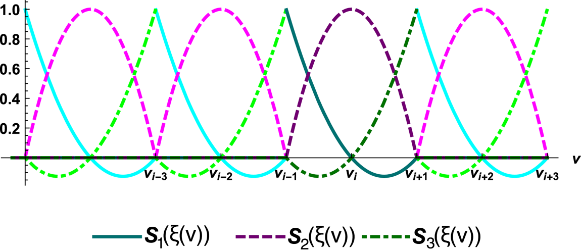
where $\xi \in [0, 1]$ and $0$ everywhere else. We define $\xi (v) = ({v - v_{i-1}})/({v_{i+1} - v_{i-1}}) = ({v - v_{i-1}})/({2 {\rm \Delta} v})$ for $v \in [v_{i-1}, v_{i+1}]$. The basis functions are illustrated in figure 1. This choice conserves particle number density because $S_1 + S_2 + S_3 = 1; \forall \, \xi \in [0, 1]$. The particle number represented by the marker particle is

(2.4)\begin{equation} {\mathcal{N}}_{\mathrm{particle}, k} = w_k,\end{equation}

and the corresponding grid particle number, mapped from the particle, is

(2.5)\begin{align} &{\mathcal{N}}_{\mathrm{grid}, i - 1} + {\mathcal{N}}_{\mathrm{grid}, i} + {\mathcal{N}}_{\mathrm{grid}, i + 1} \nonumber\\ &\quad = w_k S_1(\xi(v_k)) + w_k S_2(\xi(v_k)) + w_k S_3(\xi(v_k)) = w_k = {\mathcal{N}}_{\mathrm{particle}, k}. \end{align}

To see if the $\mathbb {P}_2$ elements conserve momentum and energy, we note the following identities:

(2.6)\begin{equation} \left.\begin{aligned} &\displaystyle S_3\left(\dfrac{v - v_{i - 1}}{2 {\rm \Delta} v}\right) - S_1\left(\dfrac{v - v_{i - 1}}{2 {\rm \Delta} v}\right) = \dfrac{v - v_i}{{\rm \Delta} v}, \\ &\displaystyle S_1\left(\dfrac{v - v_{i - 1}}{2 {\rm \Delta} v}\right) + S_3\left(\dfrac{v - v_{i - 1}}{2 {\rm \Delta} v}\right) = \dfrac{(v - v_i)^2}{({\rm \Delta} v)^2}. \end{aligned}\right\} \end{equation}

The momentum of the marker particle is

(2.7)\begin{equation} P_{\mathrm{particle}, k} = w_k v_k.\end{equation}

The corresponding grid momentum is

(2.8)\begin{align} &P_{\mathrm{grid}, i - 1} + P_{\mathrm{grid}, i} + P_{\mathrm{grid}, i + 1} \nonumber\\ &\quad = w_k S_1 (\xi (v_k ) ) v_{i-1} + w_k S_2 (\xi (v_k ) ) v_i + w_k S_3 (\xi (v_k ) ) v_{i + 1} \nonumber\\ &\quad= w_k [ (v_i - {\rm \Delta} v ) S_1 + v_i S_2 + (v_i + {\rm \Delta} v ) S_3 ] \nonumber\\ &\quad= w_k [v_i (S_1 + S_2 + S_3 ) + {\rm \Delta} v (S_3 - S_1 ) ] \nonumber\\ &\quad= w_k \left[v_i + {\rm \Delta} v \frac{v_k - v_i}{{\rm \Delta} v} \right] = w_k v_k = P_{\mathrm{particle}, k}. \end{align}

Analogously the energy of the marker particle is

(2.9)\begin{equation} E_{\mathrm{particle}, k} = w_k v_k^2,\end{equation}

and the corresponding grid energy is

(2.10)\begin{align} &E_{\mathrm{grid}, i - 1} + E_{\mathrm{grid}, i} + E_{\mathrm{grid}, i + 1} \nonumber\\ &\quad = w_k S_1 (\xi (v_k ) ) v_{i-1}^2 + w_k S_2 (\xi (v_k ) ) v_i^2 + w_k S_3 (\xi (v_k ) ) v_{i + 1}^2 \nonumber\\ &\quad = w_k [ (v_i - {\rm \Delta} v )^2 S_1 + v_i^2 S_2 + (v_i + {\rm \Delta} v )^2 S_3 ] \nonumber\\ &\quad = w_k [v_i^2 (S_1 + S_2 + S_3 ) + 2 v_i {\rm \Delta} v (S_3 - S_1 ) + ({\rm \Delta} v )^2 (S_1 + S_3 ) ] \nonumber\\ &\quad = w_k \left[v_i^2 + 2 v_i {\rm \Delta} v \frac{v_k - v_i}{{\rm \Delta} v} + ({\rm \Delta} v)^2 \frac{(v_k - v_i)^2}{({\rm \Delta} v)^2} \right] = w_k v_k^2 = E_{\mathrm{particle}, k}. \end{align}

We have thus shown that this $\mathrm {particles} \rightarrow \mathrm {grid}$ mapping preserves particle number, momentum and energy in one dimension. This is in fact the only quadratic mapping of a single particle onto a uniform grid, with three non-zero shape functions in each finite element, that will simultaneously preserve density, momentum and energy, because $S_1 (\xi )$, $S_2 (\xi )$, $S_3 (\xi )$ in (2.3) is the only solution to the system

(2.11)\begin{equation} \left.\begin{array}{ll@{}} S_1(\xi) + S_2(\xi) + S_3(\xi) = 1 & \mathrm{(particle~conservation)}, \\ 0 \times S_1(\xi) + 0.5 \times S_2(\xi) + 1.0 \times S_3(\xi) = \xi & \mathrm{(momentum~conservation)}, \\ 0^2 \times S_1(\xi) + 0.5^2 \times S_2(\xi) + 1.0^2 \times S_3(\xi) = \xi^2 & \mathrm{(energy~conservation)}. \end{array}\right\} \end{equation}

Figure 1.

Illustration of the shape functions $S_1 (\xi (v))$, $S_2 (\xi (v))$ and $S_3 (\xi (v))$ in one-dimensional v-space representing $\mathbb {P}_2$ Lagrange elements.

2.2. Two-dimensional uniform grid

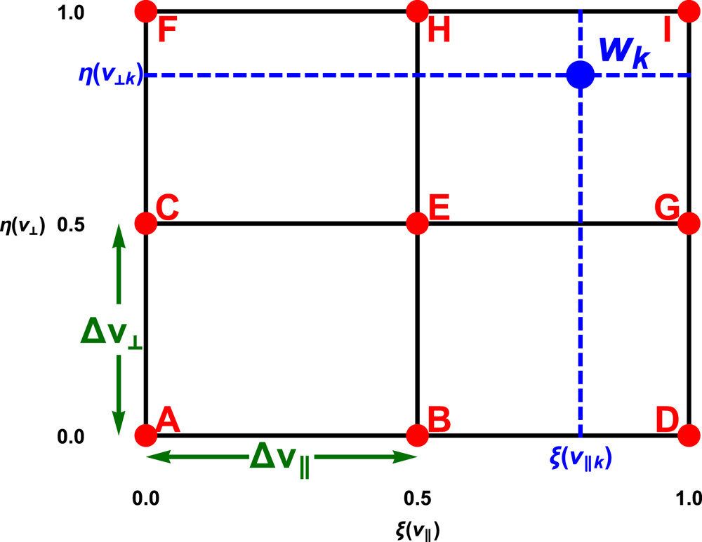
In XGC the v-space is a two-dimensional uniform rectangular grid in $v_{\|}$, $v_{\perp }$. The mapping onto the grid representation of the distribution function is described in Yoon & Chang (Reference Yoon and Chang2014) and uses the $\mathbb {P}_1$ Lagrange elements (one-dimensional shape functions $S_1(\xi ) = 1 - \xi$; $S_2(\xi ) = \xi$) which fail to preserve the energy of the marker particle representation. When extending the code to quadratic elements a finite element will encompass nine vertices as illustrated in figure 2, and we have to use an odd number of grid points in both dimensions. Analogously to the one-dimensional basis functions in (2.3), we realize that we can map the weight $w_k$ of a marker particle onto the grid using the nine two-dimensional functions obtained by combinations of the one-dimensional functions.

Figure 2.

Illustration of a finite element when using a quadratic basis in v-space for a uniform rectangular grid in $v_{\|}$, $v_{\perp }$, where we have labelled the nine vertices A, B,…, I.

To extend the bilinear mapping in Yoon & Chang (Reference Yoon and Chang2014) to a quadratic mapping, we define the coefficients

(2.12)\begin{equation} \left. \begin{aligned} &\mathcal{P}_{k \rightarrow \mathrm{A}} = S_1 (\xi (v_{\| k} ) ) S_1 (\eta (v_{{\perp} k} ) ), \\ &\mathcal{P}_{k \rightarrow \mathrm{B}} = S_2 (\xi (v_{\| k} ) ) S_1 (\eta (v_{{\perp} k} ) ), \\ &\mathcal{P}_{k \rightarrow \mathrm{C}} = S_1 (\xi (v_{\| k} ) ) S_2 (\eta (v_{{\perp} k} ) ), \\ &\mathcal{P}_{k \rightarrow \mathrm{D}} = S_3 (\xi (v_{\| k} ) ) S_1 (\eta (v_{{\perp} k} ) ), \\ & \mathcal{P}_{k \rightarrow \mathrm{E}} = S_2 (\xi (v_{\| k} ) ) S_2 (\eta (v_{{\perp} k} ) ), \\ &\mathcal{P}_{k \rightarrow \mathrm{F}} = S_1 (\xi (v_{\| k} ) ) S_3 (\eta (v_{{\perp} k} ) ), \\ &\mathcal{P}_{k \rightarrow \mathrm{G}} = S_3 (\xi (v_{\| k} ) ) S_2 (\eta (v_{{\perp} k} ) ), \\ &\mathcal{P}_{k \rightarrow \mathrm{H}} = S_2 (\xi (v_{\| k} ) ) S_3 (\eta (v_{{\perp} k} ) ), \\ & \mathcal{P}_{k \rightarrow \mathrm{I}} = S_3 (\xi (v_{\| k} ) ) S_3 (\eta (v_{{\perp} k} ) ),\end{aligned} \right\}\end{equation}

describing the fraction of weight $\mathcal {P}_{k \rightarrow \beta }$ distributed from particle $k$ onto grid vertex $\beta$, and where we have labelled the grid vertices as in figure 2 and defined the normalized velocity coordinates $\xi (v_\|) = ({v_\| - v_{\|, i-1}})/({v_{\|, i+1} - v_{\|, i-1}}) \in [0, 1]$ and $\eta (v_\perp ) = ({v_\perp - v_{\perp , j-1}})/({v_{\perp , j+1} - v_{\perp , j-1}}) \in [0, 1]$ in the two-dimensional velocity cell where the particle is located. For the $N_p$ marker particles residing within a two-dimensional cell, the v-space representation of the distribution can be expressed as

(2.13)\begin{equation} f_{\mathrm{particle}}(v_\|, v_\perp) = \sum_{k = 1}^{N_p} \frac{w_k}{V_k} \delta(v_\| - v_{\| k}, v_\perp{-} v_{{\perp} k}).\end{equation}

We can then use the mapping in (2.12) to obtain the corresponding grid distribution of vertex $\beta$ as

(2.14)\begin{equation} f_{\mathrm{grid}, \beta} = \frac{1}{V_{\beta}} \sum_{k = 1}^{N_p} w_k \mathcal{P}_{k \rightarrow \beta}, \end{equation}

where $V_{\beta } = 2 {\rm \pi}v_{\perp \beta } {\rm \Delta} v_{\perp } {\rm \Delta} v_{\|}$ is the v-space volume of the vertex. The form of the v-space volume originates from the Jacobian when $v_{\perp }$, $v_{\|}$ represent cylindrical velocity coordinates and after integrating over gyro-phase angle at constant ‘gyrocentre’ position. It is straightforward to verify that this mapping conserves particle number

(2.15)\begin{equation} \mathcal{P}_{k \rightarrow \mathrm{A}} + \mathcal{P}_{k \rightarrow \mathrm{B}} + \cdots + \mathcal{P}_{k \rightarrow \mathrm{I}} = 1, \end{equation}

parallel momentum

(2.16)\begin{equation} v_{\| \mathrm{A}} \mathcal{P}_{k \rightarrow \mathrm{A}} + v_{\| \mathrm{B}} \mathcal{P}_{k \rightarrow \mathrm{B}} + \cdots + v_{\| \mathrm{I}} \mathcal{P}_{k \rightarrow \mathrm{I}} = v_{\| k}, \end{equation}

perpendicular momentum

(2.17)\begin{equation} v_{{\perp} \mathrm{A}} \mathcal{P}_{k \rightarrow \mathrm{A}} + v_{{\perp} \mathrm{B}} \mathcal{P}_{k \rightarrow \mathrm{B}} + \cdots + v_{{\perp} \mathrm{I}} \mathcal{P}_{k \rightarrow \mathrm{I}} = v_{{\perp} k} \end{equation}

and energy

(2.18)\begin{equation} (v_{\| \mathrm{A}}^2 + v_{{\perp} \mathrm{A}}^2 ) \mathcal{P}_{k \rightarrow \mathrm{A}} + (v_{\| \mathrm{B}}^2 + v_{{\perp} \mathrm{B}}^2 ) \mathcal{P}_{k \rightarrow \mathrm{B}} + \cdots + (v_{\| \mathrm{I}}^2 + v_{{\perp} \mathrm{I}}^2 ) \mathcal{P}_{k \rightarrow \mathrm{I}} = v_{\| k}^2 + v_{{\perp} k}^2, \end{equation}

but we omit the details here.

After the Coulomb collision operation, and other source operations, we obtain an updated grid distribution $f_{\mathrm {grid}, \beta }^{\mathrm {new}}$. It is possible to execute the inverse mapping back from vertex $\beta$ to particle $\alpha$ using the coefficient

(2.19)\begin{equation} \mathcal{P}_{\beta \rightarrow \alpha}^{({-}1)} = \frac{\mathcal{P}_{\alpha \rightarrow \beta}}{\displaystyle \sum_{k = 1}^{N_p} \mathcal{P}_{k \rightarrow \beta}}, \end{equation}

and update the new weight of the particle as

(2.20)\begin{equation} w_\alpha^{\mathrm{new}} = \sum_{\beta} f_{\mathrm{grid}, \beta}^{\mathrm{new}} V_{\beta} \mathcal{P}_{\beta \rightarrow \alpha}^{({-}1)}. \end{equation}

This inverse mapping is a direct extension of the bilinear scheme in XGC.

Although this simple quadratic mapping theoretically will work, it has two major drawbacks. Firstly, the inverse mapping given by (2.19) and (2.20) will not result in exact momentum and energy conservation when moving from the grid representation to the marker particle representation after an operation on $f_{\mathrm {grid}}$ on the velocity grid. Secondly, and more severely, in contrast to the bilinear scheme, the mapping coefficients in (2.12) can be negative. As a consequence, when doing the inverse mapping the denominator in (2.19) can become arbitrarily close to 0 resulting in numerical issues. In the next section we introduce a way to overcome these issues using a pseudo-inverse.

Readers may question why negative particle-mapping coefficients are allowed at all since this can lead to a negative value of particles ($f_p$) on some velocity grids according to (2.14). However, a negative grid distribution of particles on some velocity grids is not a problem as long as the total distribution function (including $f_0$) in (1.1) stays positive. In fact, the $w_{1,k}$ weights, described after (2.1), can have either sign in XGC.

However, discretization effects in the particle and v-space grid interpolation with not enough number of particles for every v-space could induce negative v-space mesh values of the total $f_s$ at high energy, where $f_0$ is small, but their contribution to the physics is negligible. Our particle resampling technique (discussed in § 3), which creates particles in the needed phase space, further mitigates this issue. In XGC, if negative values of the total distribution at some high-energy grid nodes do appear, they are replaced by negligibly small, positive values (about $10^{-2}$ of the Maxwellian background value at the local velocity grid node). Additionally, if our v-space dissipative operations (such as Fokker–Planck collisions) create a negative $f_s$ value at high energy, where the $f_s$ values can be noisy due to lack of enough particles, a constrained quadratic programming optimization is used to relax $f_s + ({\rm \Delta} f_s)_{\mathrm {coll}}$ on an extended $3 \times 3$ grid containing the grid point to a Maxwellian while conserving mass, momentum and energy. The error created by these negativity-mitigation operations is negligible compared to the accuracy required in the physics calculation, as can be noticed in the example physics figures presented in § 4. We close by noting that the negativity issue of the velocity grid $f_s$ discussed in this paragraph is not relevant to the theme of this paper, which is confined to an accurate interpolation method that satisfies the conservation constraints between particles and velocity grid.

3. Novel velocity mapping technique

In this section we describe a different method to map marker particle weights back and forth between particle positions and the velocity grid which avoids the problem of singularities described in the previous section, and enables exact conservation of moments up to the order of the finite element space. Assume a particle distribution of $N_p$ particles

(3.1)\begin{equation} \bar{f}_{\mathrm{particle}} (\boldsymbol{v} ) = \sum_{k = 1}^{N_p} w_k \delta (\boldsymbol{v} - {\boldsymbol{v}_{k}} ),\end{equation}

a finite element space $\mathcal {F}$ and a function $u \in \mathcal {F}$. Since we are effectively mapping particle weights rather than particle densities, we choose to omit the v-space volume that is present in (2.2) and (2.13) in the definition in (3.1). Hence the overbar notation is used to distinguish it from a regular distribution function. We would like to have a unique $u = \bar {f}_{\mathrm {particle}}(\boldsymbol {v});~\forall \,\boldsymbol {v}$, but this is not possible unless $\bar {f}_\textrm {particle} \in \mathcal {F}$. Instead we write

(3.2)\begin{equation} u = \sum_{j} c_j \phi_j,\end{equation}

where the functions $\phi _j (\boldsymbol {v})$ form a complete basis of $\mathcal {F}$, and look for a solution that fulfils weak equivalence

(3.3)\begin{equation} \int\, \mathrm{d}\boldsymbol{v} \phi_i \bar{f}_{\mathrm{particle}} = \int\, \mathrm{d}\boldsymbol{v} \phi_i u, \end{equation}

for all $\phi _i \in \mathcal {F}$ (i.e. we find the projection of $\bar {f}_{\mathrm {particle}}$ onto the function space $\mathcal {F}$). Note that the left-hand side of (3.3) is simply obtained by evaluating the particle positions in the basis functions.

We define a finite element mass matrix

(3.4)\begin{equation} \boldsymbol{\mathsf{M}}_{ij} = \int \mathrm{d}\boldsymbol{v} \phi_i \phi_j \end{equation}

and a matrix set by the particle positions

(3.5)\begin{equation} \boldsymbol{\mathsf{V}}_{jk} = \phi_j (\boldsymbol{v}_{k}).\end{equation}

We can then write weak equivalence as

(3.6)\begin{equation} \boldsymbol{\mathsf{M}} \boldsymbol{c} = \boldsymbol{\mathsf{V}} \boldsymbol{w}, \end{equation}

where we have defined the vector $\boldsymbol {w}$ by the particle weights in (3.1) and the vector $\boldsymbol {c}$ by the coefficients in (3.2) (Hirvijoki & Adams Reference Hirvijoki and Adams2017). Here ${\boldsymbol{\mathsf{M}}}$ is a sparse invertible square matrix of size equal to the number of basis functions, which in practice is equal to the number of grid points on the velocity grid, $N_g \times N_g$. The sparsity follows from the fact that most pairs of basis functions have no overlapping support. Similarly ${\boldsymbol{\mathsf{V}}}$ is also a sparse matrix because a particle position evaluated in a basis function will only be non-zero for the basis functions of the element in which the particle resides. Matrix ${\boldsymbol{\mathsf{V}}}$ is rectangular of size $N_g \times N_p$ generally with the same number of non-zero matrix entries per column as there are grid vertices per element (i.e. 4 for linear elements or 9 for quadratic elements) and each column sums to 1. In the typical case of more particles than grid points, $N_p > N_g$, ${\boldsymbol{\mathsf{V}}}$ is a short fat matrix (in our implementation described here this is practically always the case due to the particle resampling described later), but it could in principle also be a square or tall skinny matrix if the particle count is very low.

To map the weights from the marker particle representation of the distribution function to the grid representation we simply use

(3.7)\begin{equation} \bar{f}_{\mathrm{grid}} = \boldsymbol{\mathsf{V}} \boldsymbol{w},\end{equation}

and the coefficients of the basis functions become

(3.8)\begin{equation} \boldsymbol{c} = \boldsymbol{\mathsf{M}}^{{-}1} \boldsymbol{\mathsf{V}} \boldsymbol{w}.\end{equation}

After applying grid operations we note from (3.6) that it would be possible to map back to the particle representation using ${\boldsymbol{\mathsf{V}}}^{\mathrm {T}} {\boldsymbol{\mathsf{M}}} \boldsymbol {c}_{\mathrm {new}}$, where the superscript ‘$\mathrm {T}$’ denotes the transpose and the subscript ‘new’ refers to after the grid operations, but this does not preserve the moments. Instead we compute the new particle weights $\boldsymbol {w}_{\mathrm {new}}$ using an inverse of ${\boldsymbol{\mathsf{V}}}$, but this inverse is not well defined. We have to resort to a pseudo-inverse, ${\boldsymbol{\mathsf{V}}}^{+}$.

In the unlikely case of fewer particles than grid points, $N_p < N_g$, we can use

(3.9)\begin{equation} \boldsymbol{\mathsf{V}}^{+} = (\boldsymbol{\mathsf{V}}^{\mathrm{T}} \boldsymbol{\mathsf{V}})^{{-}1} \boldsymbol{\mathsf{V}}^{\mathrm{T}},\end{equation}

which is a left inverse since ${\boldsymbol{\mathsf{V}}}^{+} {\boldsymbol{\mathsf{V}}} = {\boldsymbol{\mathsf{I}}}$, the identity matrix. If we were to map back and forth using the left inverse with an identity operation on the grid, e.g. no operation, we would end up with the new weights $\boldsymbol {w}_{\mathrm {new}} = ({\boldsymbol{\mathsf{V}}}^{\mathrm {T}} {\boldsymbol{\mathsf{V}}})^{-1} {\boldsymbol{\mathsf{V}}}^{\mathrm {T}} {\boldsymbol{\mathsf{V}}} \boldsymbol {w} = \boldsymbol {w}$, i.e. we would recover the original weights without losing any information. However, for the typical case of more particles than grid points, $N_p > N_g$, we have to use the right inverse, ${\boldsymbol{\mathsf{V}}} {\boldsymbol{\mathsf{V}}}^{+} = {\boldsymbol{\mathsf{I}}}$, given by the Moore–Penrose inverse (Penrose Reference Penrose1955)

(3.10)\begin{equation} \boldsymbol{\mathsf{V}}^{+} = \boldsymbol{\mathsf{V}}^{\mathrm{T}} (\boldsymbol{\mathsf{V}} \boldsymbol{\mathsf{V}}^{\mathrm{T}})^{{-}1}, \end{equation}

and update the new particle weights as

(3.11)\begin{equation} \boldsymbol{w}_{\mathrm{new}} = \boldsymbol{\mathsf{V}}^{\mathrm{T}} (\boldsymbol{\mathsf{V}} \boldsymbol{\mathsf{V}}^{\mathrm{T}})^{{-}1} \boldsymbol{\mathsf{M}} \boldsymbol{c}_{\mathrm{new}}.\end{equation}

This transformation preserves the moments up to the order of the finite elements as demonstrated by Hirvijoki et al. (Reference Hirvijoki, Kraus and Burby2018).

If we again were to map back and forth with an identity operation on the grid we would end up with the new weights $\boldsymbol {w}_{\mathrm {new}} = {\boldsymbol{\mathsf{V}}}^{\mathrm {T}} ({\boldsymbol{\mathsf{V}}} {\boldsymbol{\mathsf{V}}}^{\mathrm {T}})^{-1} {\boldsymbol{\mathsf{V}}} \boldsymbol {w}$. This implies that the particle weights have changed, i.e. although the moments are conserved we will unavoidably lose information. The fact that we will generally lose information when $N_p > N_g$, unless there is a specific structure in the particle data that we can exploit, follows from the impossibility of always recovering a larger set of data in the particles from a smaller set of data in the grid points (i.e. we cannot use the left inverse when $N_p > N_g$ except if the operand happens to be in the span of ${\boldsymbol{\mathsf{V}}}^{\mathrm {T}}$).

If we apply the right pseudo-inverse mapping back and forth twice with an identity grid operation we obtain $\boldsymbol {w}_{\mathrm {new}} = {\boldsymbol{\mathsf{V}}}^{\mathrm {T}} ({\boldsymbol{\mathsf{V}}} {\boldsymbol{\mathsf{V}}}^{\mathrm {T}})^{-1} {\boldsymbol{\mathsf{V}}} {\boldsymbol{\mathsf{V}}}^{\mathrm {T}} ({\boldsymbol{\mathsf{V}}} {\boldsymbol{\mathsf{V}}}^{\mathrm {T}})^{-1} {\boldsymbol{\mathsf{V}}} \boldsymbol {w} = {\boldsymbol{\mathsf{V}}}^{\mathrm {T}} ({\boldsymbol{\mathsf{V}}} {\boldsymbol{\mathsf{V}}}^{\mathrm {T}})^{-1} {\boldsymbol{\mathsf{V}}} \boldsymbol {w}$, i.e. the same result as when mapping only once. The process is idempotent since no more information is lost when applying the operation several times. Moreover, we point out that the conservation properties of the pseudo-inverse mapping follow naturally from the preserving structure of the mapping and the conservation is local in all phase-space cells. It is simpler to implement a velocity-global conservation only, in the interpolation between velocity grid and particles while neglecting the details of the v-space distribution, but this would mean that we lose the fidelity of kinetic dynamics. For example, the velocity structure change of the particle distribution function local to near the trapped–passing boundary in v-space has a critical effect on the radial transport in tokamak plasmas.

A numerical implementation of the described mapping technique with the pseudo-inverse is included in the petsc library, version 3.14 (Balay et al. Reference Balay2020). We use petsc to implement a new velocity interpolation in XGC with the linear first-order $\mathbb {P}_1$ Lagrange elements or the quadratic second-order $\mathbb {P}_2$ elements as basis functions. It would be a straightforward extension to implement even higher-order elements, but our target is to achieve energy conservation for which second-order elements suffice – as is the case for the XGC simulations. We leave it to future work to explore whether other higher-order basis functions than the Lagrange basis would also provide the sought-for conservation properties, e.g. the B-splines that are commonly used for interpolation in configuration space.

The ‘$\mathrm {particles} \rightarrow \mathrm {grid}$’ mapping merely consists of constructing the ${\boldsymbol{\mathsf{M}}}$, ${\boldsymbol{\mathsf{V}}}$ matrices, the weights vector $\boldsymbol {w}$ and performing matrix multiplications. With $\mathbb {P}_1$ elements this operation gives the same result as the former XGC velocity interpolation, whereas $\mathbb {P}_2$ elements result in a mapping equivalent to (2.14) (taking the v-space volumes into account).

The inverse ‘$\mathrm {grid} \rightarrow \mathrm {particles}$’ mapping is more critical because it involves constructing the pseudo-inverse using an iterative Krylov solver in petsc. This operation can fail if $({\boldsymbol{\mathsf{V}}} {\boldsymbol{\mathsf{V}}}^{\mathrm {T}})^{-1}$ in (3.11) is not well-posed, which can happen (but not necessarily) when there are basis functions without any particles. To ensure that the pseudo-inverse calculation will always work, we have to ensure that all cells on the velocity grid, in all real-space mesh vertices, are populated by particles. In XGC simulations, with a realistic number of marker particles and a typical 5-D grid size, we expect that a fraction $\sim 1\,\%$ of all velocity cells are not appropriately populated during a time step, and particularly cells at high kinetic energy. To remedy this issue, XGC is equipped with a particle resampling technique which is used to create, annihilate or redistribute particles in configuration space while preserving a desired number of moments (Faghihi et al. Reference Faghihi, Carey, Michoski, Hager, Janhunen, Chang and Moser2020). (More details of the XGC resampling can be found in Dominski et al. (Reference Dominski2021).) Here, we use the particle resampling technique to fill up v-space by marker particles where needed. We apply the resampling just before the ‘$\mathrm {particles} \rightarrow \mathrm {grid}$’ mapping to ensure that the pseudo-inverse can always be calculated, i.e. the mapping is always well-posed. Since the resampling will fill all empty velocity cells appropriately with particles, we will practically never end up in a situation where $N_p < N_g$ as long as we initiate the simulation with enough particles while using the built-in load-balancing technique of XGC. Particle noise is also controlled by application of the particle resampling technique.

4. Application to a neoclassical XGC simulation

Here we apply the new velocity mapping described in § 3 to a circular cross-sectional tokamak neoclassical test case for XGC, the same case as in Hager, Dominski & Chang (Reference Hager, Dominski and Chang2019), but for simplicity we use adiabatic instead of kinetic electrons, and demonstrate the improved conservation properties of the interpolation. Note that no significant influence of the different interpolation methods on the physical observables is expected in this test case due to its mild density and temperature gradients. Our objective is rather to demonstrate that the new implementation reduces the interpolation error to a negligible level. Therefore, we focus on the Fokker–Planck collision error and the particle to/from velocity grid interpolation error. Even if the interpolation errors are too small to influence the physical simulation results here, it is always desirable to have interpolation errors that are smaller than the velocity grid collision errors. In realistic edge cases with steep pedestal profiles, the interpolation errors are typically larger and can cause numerical issues if they are too large.

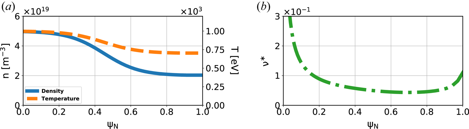
In the comparison we refer to the former XGC velocity mapping as the ‘bilinear’ implementation, whereas we call the new mapping first- and second-order ‘pseudo-inverse’, respectively. We will omit the species index in the presented results because all quantities are for the main deuterium ions with mass $m$. The input plasma profiles of density $n$, temperature $T$ and collisionality at the beginning of the simulations are illustrated in figure 3 as a function of normalized poloidal flux $\psi _N$, which is a minor radial coordinate. The collisionality is defined as ${\nu }^{\ast } = q R \nu / ({\epsilon }^{3/2} v_{T})$ with safety factor $q$, major radius $R$, inverse aspect ratio $\epsilon$, thermal velocity $v_{T} = \sqrt {2 T / m}$ and $90^{\circ }$ collision frequency $\nu$ (Helander & Sigmar Reference Helander and Sigmar2002). The profiles are free to evolve during a simulation, but because the simulated time is much shorter than the neoclassical core transport time scale they remain practically unchanged. The three-dimensional configuration space mesh consists of 6368 nodes, the velocity grid has $45 \times 45$ nodes and the simulation domain is set to $\psi _N < 0.9$. In neoclassical tokamak XGC simulations, a single poloidal plane is used because of axisymmetry. The total number of particles is ${\sim }30$ million throughout the simulations but varies $\pm 5$ % because of the particle resampling. We run 400 time steps of length ${\rm \Delta} t = 0.28\ \mathrm {\mu }\mathrm {s}$, which is about six toroidal transit times of the thermal ions in the middle of the pressure slope, and study the errors. In our simulations we monitor the particle noise, characterized by the marker-particle weight variance, to check that the ‘pseudo-inverse’ mapping does not induce a large noise level. We define the collisional change in density, parallel momentum and energy during a time step of the simulation as

(4.1)\begin{equation} \left.\begin{aligned} &\displaystyle {\rm \Delta} n = {\rm \Delta} t \int C_{ii}\, \mathrm{d}^3 v,\\ &\displaystyle {\rm \Delta} P_{\|} = {\rm \Delta} t \int m v_{\|} C_{ii}\, \mathrm{d}^3 v,\\ &\displaystyle {\rm \Delta} E = {\rm \Delta} t \int \dfrac{1}{2} m v^2 C_{ii}\, \mathrm{d}^3 v,\end{aligned}\right\}\end{equation}

where $C_{ii} = ({\mathrm {d}f}/{\mathrm {d}t})_{\mathrm {coll}}$ is the ion–ion collision operator acting on the distribution function. The Fokker–Planck–Landau collision operator implemented in XGC conserves particle density (${\rm \Delta} n = 0$), parallel momentum (${\rm \Delta} P_{\|} = 0$) and kinetic energy (${\rm \Delta} E = 0$) up to a user-defined accuracy for a single-ion-species simulation (in a multi-species simulation all interspecies collisions must also be considered and the total momentum and energy are conserved instead). We therefore let the numerical error of a quantity be the absolute value of the corresponding change in the quantity (however, in the colour map plots to be shown, we leave the sign).

Figure 3.

Input plasma profiles of (a) ion density and temperature and (b) collisionality.

The collision operation in the code is implemented with an implicit time discretization that is solved iteratively until the desired conservation error tolerances are met. This implies that the collision errors can be made arbitrarily small down to machine precision by choosing stricter tolerances (and potentially a smaller time step). However, since the collision operation can be a substantial fraction of the total computing time, the tolerances are set such that the errors are small enough to limit the number of iterations while keeping the accumulated conservation error at an acceptable level over the required number of time steps. In contrast to the particle to/from velocity grid interpolation, the collision operator does not conserve perpendicular momentum.

While the collision errors are calculated by examining the changes on the velocity grid, the interpolation errors have to be calculated using the marker particle representation. The interpolation errors are therefore computed using the total changes of mass, momentum and energy in the full process ‘$\mathrm {particles} \rightarrow \mathrm {grid}$’ mapping, collisions, ‘$\mathrm {grid} \rightarrow \mathrm {particles}$’ mapping, and then subtracting the collision errors.

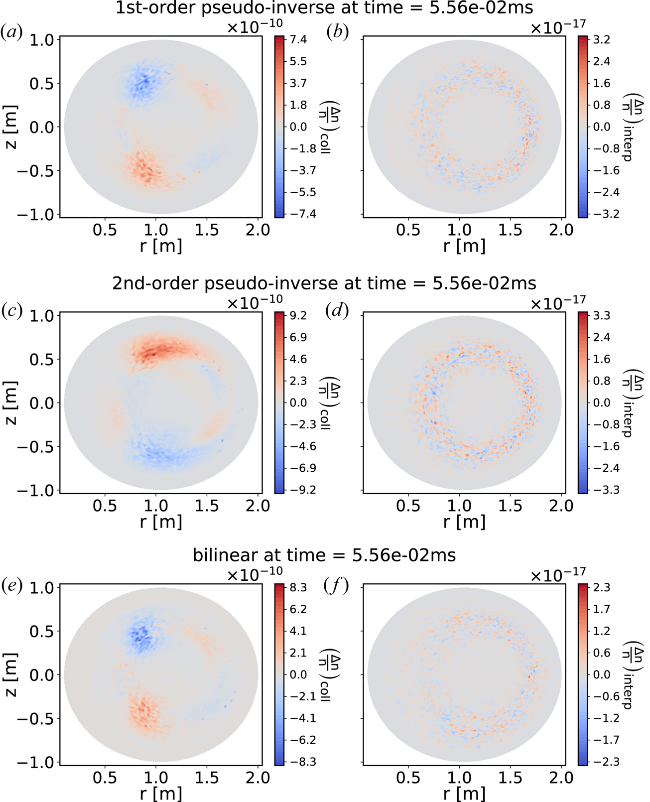
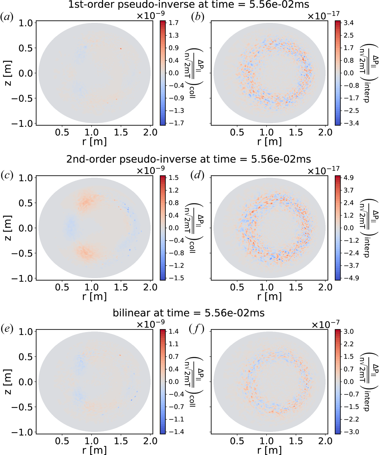
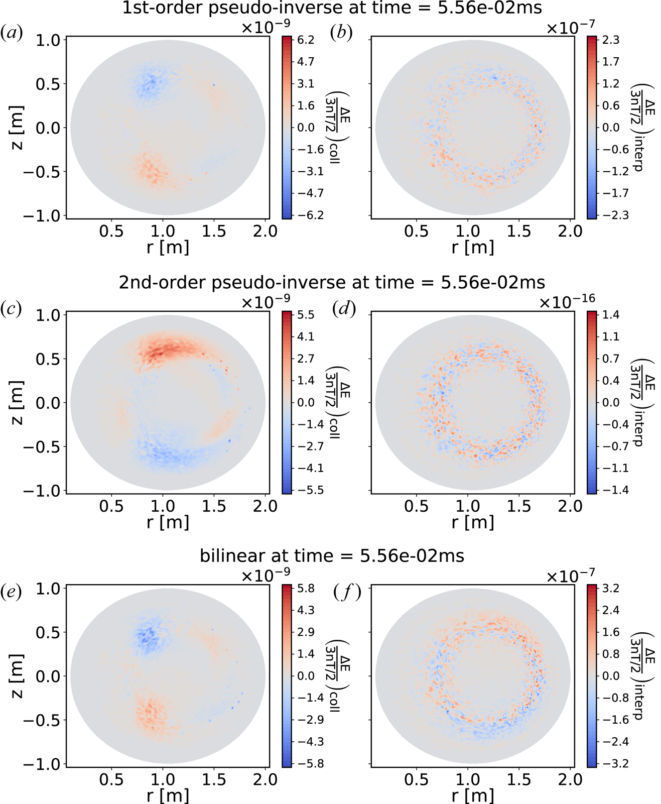
In figures 4–6 we show the poloidal cross-section of the normalized density error, the normalized parallel momentum error and the normalized kinetic energy error for the Coulomb collision operation and the velocity interpolation calculated in each configuration space vertex in a time step of the simulation. The relative density, momentum and energy errors are normalized to background density $n$, momentum at thermal speed $m n v_{T} = n \sqrt {2 m T}$ and pressure $3 n T / 2$, respectively.

Figure 4.

Colour maps of the change in relative ion density ${\rm \Delta} n / n$ (relative density error) in all configuration space vertices of the poloidal cross-section in time step 200 of the simulation. The colour maps show the change due to the collisions (a,c,e) and the change due to the interpolation (b,d,f), comparing the three different velocity mapping methods: first-order ‘pseudo-inverse’ (a,b), second-order ‘pseudo-inverse’ (c,d) and ‘bilinear’ (e,f).

Figure 5.

Colour maps of the change in linear parallel momentum normalized to momentum at thermal speed ${{\rm \Delta} P_{\|}}/({n \sqrt {2 m T}})$ (relative parallel momentum error) for the ions in all configuration space vertices of the poloidal cross-section in time step 200 of the simulation. The colour maps show the change due to the collisions (a,c,e) and the change due to the interpolation (b,d,f), comparing the three different velocity mapping methods: first-order ‘pseudo-inverse’ (a,b), second-order ‘pseudo-inverse’ (c,d) and ‘bilinear’ (e,f).

Figure 6.

Colour maps of the change in kinetic energy normalized to pressure ${{\rm \Delta} E}/{(3 n T / 2)}$ (relative energy error) for the ions in all configuration space vertices of the poloidal cross-section in time step 200 of the simulation. The colour maps show the change due to the collisions (a,c,e) and the change due to the interpolation (b,d,f), comparing the three different velocity mapping methods: first-order ‘pseudo-inverse’ (a,b), second-order ‘pseudo-inverse’ (c,d) and ‘bilinear’ (e,f).

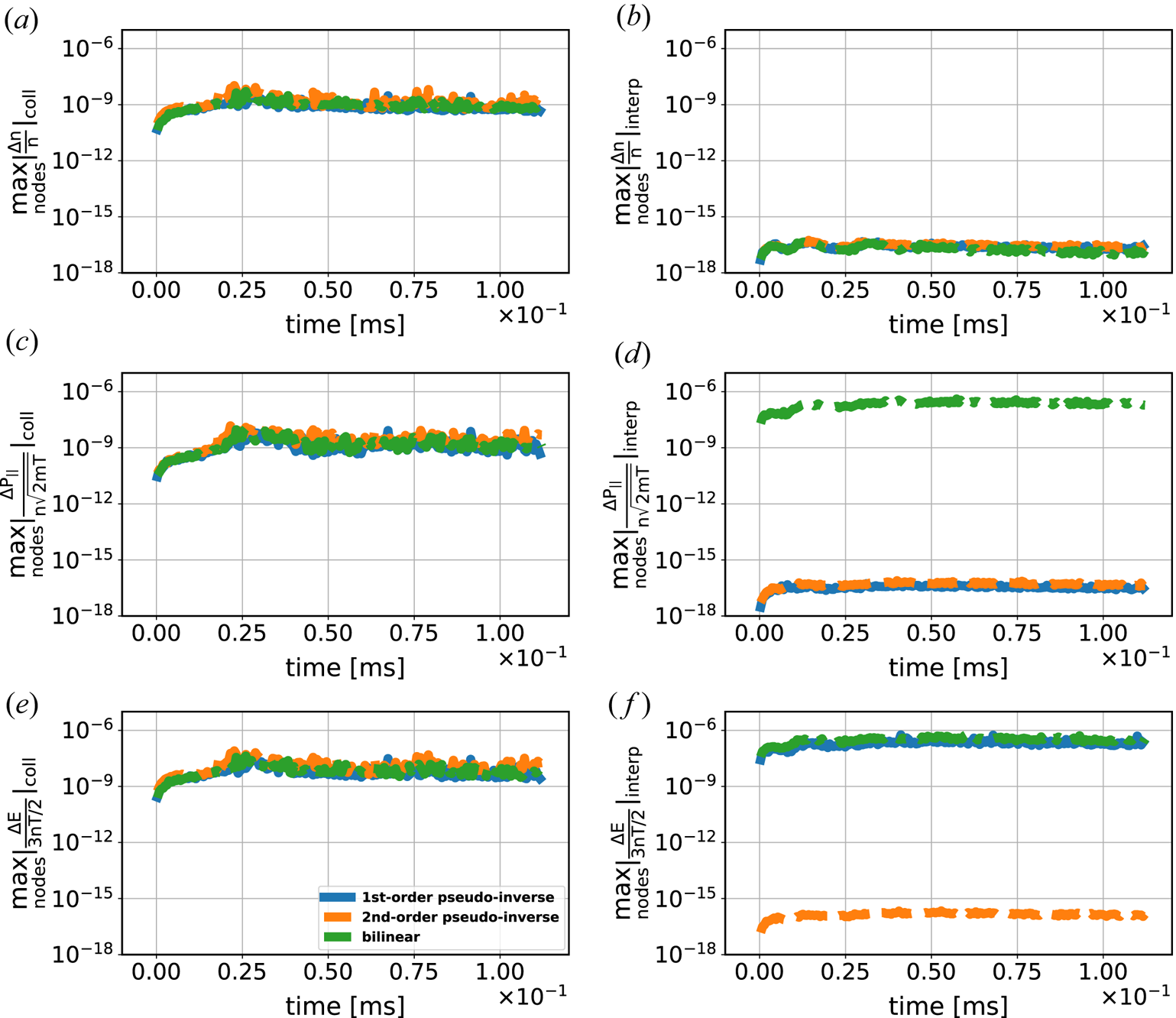
Figure 4 shows that all three velocity mapping methods exhibit a much smaller interpolation density error than collision density error. This implies that the change in density from the collision operation seen in the marker particle representation is unaffected by the velocity interpolation. Note that since the marker particle weights in the ‘$\mathrm {grid} \rightarrow \mathrm {particles}$’ mapping are distributed differently depending on the method used, we cannot expect the collision error to look exactly the same when comparing between the different methods. What matters is that the error remains of the same size and the interpolation error is significantly smaller. For the momentum error in figure 5 we see that the ‘pseudo-inverse’ methods have a much smaller interpolation error than the ‘bilinear’ method. In fact, there are configuration space vertices where the ‘bilinear’ method results in a larger interpolation error than the collision error. This is not ideal from a numerical point of view, even though the total error in the marker particle representation remains smaller than required by XGC. The test case here has relatively benign properties with mild gradients and the interpolation error could be larger for realistic geometry and high-confinement mode profiles. However, it is possible to control the error by the number of marker particles in the simulation (Hager et al. Reference Hager, Yoon, Ku, D'Azevedo, Worley and Chang2016). As expected from theory, figure 6 illustrates that the quadratic second-order ‘pseudo-inverse’ method exhibits an interpolation error in kinetic energy that is negligible compared to the collision error. In contrast, for the two linear methods the interpolation error dominates over the collision error. In the figure we see that configuration space vertices located around mid-radius, where the pressure gradient is larger in the plasma (see figure 3), generally show a larger interpolation error. Figures 4–6 only illustrate the errors in a single time step. To demonstrate a consistently reduced interpolation error with the ‘pseudo-inverse’ methods we show the time evolution of the maximum relative errors in any configuration space vertex in figure 7. The collision errors in figure 7(a,c,e), controlled by the tolerances in XGC, are well below $10^{-7}$ throughout the simulation. The relative density error in the interpolation is consistently much smaller for all three methods, but the maximum momentum and energy errors are always larger than the corresponding collision errors for the ‘bilinear’ mapping. The ‘pseudo-inverse’ mappings perform as expected. The first-order mapping results in a negligible momentum error in the interpolation but the energy error is of the same size as for the ‘bilinear’ mapping. The second-order mapping shows negligible interpolation errors in both momentum and energy for all time steps. From figure 7 it is evident that the ‘pseudo-inverse’ methods maintain the reduced interpolation errors throughout the simulations without them being destroyed by ill-posedness or the increase of particle noise (see figure 8). We can thus conclude that the new velocity mapping implementation in XGC works as expected. The energy error caused by the bilinear interpolation between v-space grid and particles in the core-region example shown here is not significant. However, in the steep edge pedestal, this error could become significant. How much error we could get in the pedestal physics observables from the bilinear interpolation error and how the present quadratic pseudo-inverse interpolation can correct them will be the subject of a subsequent report.

Figure 7.

Time evolution of the maximum relative density error (a,b), maximum relative parallel momentum error (c,d) and maximum relative kinetic energy error (e,f) in any configuration space vertex (node) for the Coulomb collision operation (a,c,e) and the velocity interpolation (b,d,f), comparing the three different velocity mapping methods: first-order ‘pseudo-inverse’ (solid, blue), second-order ‘pseudo-inverse’ (dashed, orange) and ‘bilinear’ (dot-dashed, green).

Figure 8.

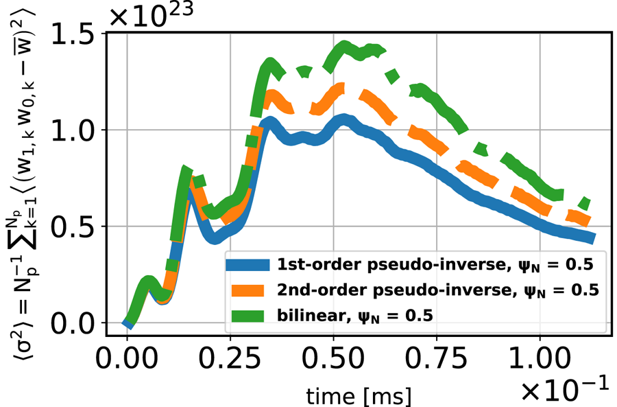
Time behaviour of the particle noise, represented by the flux-surface averaged variance of the particle weights $\langle \sigma ^2 \rangle = ({1}/{N_p}) \sum _{k = 1}^{N_p} \langle (w_{1,k} w_{0,k} - \bar {w} )^2 \rangle$, with the mean $\bar {w} = ({1}/{N_p}) \sum _{k = 1}^{N_p} w_{1,k} w_{0,k}$, at half minor radius in the normalized radial coordinate system, comparing the three different velocity mapping methods: first-order ‘pseudo-inverse’ (solid, blue), second-order ‘pseudo-inverse’ (dashed, orange) and ‘bilinear’ (dot-dashed, green). It can be observed that the particle resampling method controls well the particle noise.