





1. Introduction
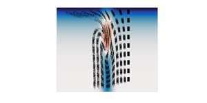
Internal solitary waves (henceforth ISWs) are long-lived features that are ubiquitously observed in natural waters (see the three reviews Helfrich & Melville Reference Helfrich and Melville2006; Lamb Reference Lamb2014; Boegman & Stastna Reference Boegman and Stastna2019 for more complete descriptions of field measurements). Mathematically, they are described by a single, elliptic eigenvalue problem; the Dubreil–Jacotin Long (DJL) equation; which is formally equivalent to the full stratified Euler equations (Stastna Reference Stastna2022). Due to their ability to propagate largely unchanged over hundreds of kilometres, and their fundamentally nonlinear nature, ISWs serve as a counterpoint to the turbulent cascade which spreads energy across length scales.
A number of numerical methods have been developed for the DJL equation (Turkington, Eydeland & Wang Reference Turkington, Eydeland and Wang1991; Stastna & Lamb Reference Stastna and Lamb2002; King, Carr & Dritschel Reference King, Carr and Dritschel2011) with the optimization theory-based methods originally due to Turkington (Turkington et al. Reference Turkington, Eydeland and Wang1991) providing a variational characterization when there is no background shear current: an ISW minimizes kinetic energy when the available potential energy is held fixed. In practice, ISWs can be computed in under a minute and all Eulerian fields can be computed a posteriori facilitating clean initializations in time-dependent numerical models as well as theoretical calculations (Dunphy, Subich & Stastna Reference Dunphy, Subich and Stastna2011).
When a background shear current is present, the algebraic complexity of the DJL equation increases considerably. The variational algorithm can be modified for this situation, and waves can again be computed rapidly. However, some of the rigorous convergence results have not, to date, been derived, and the physical interpretation of the algorithm in terms of energy no longer applies. Nevertheless, the presence of a background shear current has been shown to change the value and nature of the upper bound on wave amplitude, and can even change the wave polarity. The interplay between shear instability and internal waves, while outside the realm of steady theory, has led to a variety of interesting numerical explorations (Fructus et al. Reference Fructus, Carr, Grue, Jensen and Davies2009; Lamb & Farmer Reference Lamb and Farmer2011; Passaggia, Helfrich & White Reference Passaggia, Helfrich and White2018; Xu, Stastna & Deepwell Reference Xu, Stastna and Deepwell2019) with open questions, especially in three dimensions remaining unanswered.
Lagrangian-based models have been applied to ISWs without a background shear current (Lamb Reference Lamb1997; Scotti & Pineda Reference Scotti and Pineda2007; Stastna et al. Reference Stastna, Poulin, Subich and Mecking2011), with implications for transport as well as plankton behaviour. The ease of Lagrangian calculations leads to large data sets, and these can provide fertile ground for modern, data-centric analysis methods (e.g. Kutz & Kutz Reference Kutz2013) that differ in structure and methodology from the Eulerian methods (e.g. perturbation theoretic Grimshaw Reference Grimshaw2001) available in the literature.
The type of data generated by Lagrangian calculations naturally leads to links with the field of graph theory. Graph theory is a fundamental field of modern mathematics, and due to this universal nature, has had a broad and extensive application to fluid mechanics. For Lagrangian calculations, examples include the application of network theory, in particular sparsification, to the study of point vortices (Nair & Taira Reference Nair and Taira2015), and the application of graph colouring to the detection of coherent structures (Schlueter-Kuck & Dabiri Reference Schlueter-Kuck and Dabiri2017), which was subsequently used as a metric for Lagrangian data assimilation (Schlueter-Kuck & Dabiri Reference Schlueter-Kuck and Dabiri2019). A qualitatively different branch of graph theoretic applications in fluid mechanics involves numerical methods (finite element based) developed based on the Bond graph (Baliño Reference Baliño2009). The broader field of Bond graph applications is surveyed in the monograph by Thoma (Reference Thoma2016). In the context of applied environmental fluid mechanics, graph theory finds broad application in the characterization of ecological communities, (Treml et al. Reference Treml, Halpin, Urban and Pratson2008) being a well-quoted example for larval dispersal and hydrodynamic connectivity in an ocean setting.
In the present context, and building on the existing literature (Froyland & Padberg-Gehle Reference Froyland and Padberg-Gehle2015; Froyland & Santitissadeekorn Reference Froyland and Santitissadeekorn2017; Padberg-Gehle & Schneide Reference Padberg-Gehle and Schneide2017; Chakraborty, Coutino & Stastna Reference Chakraborty, Coutino and Stastna2019), we report on the application of graph theoretic methods to contrast ISWs with and without a shear current. We find that graphs provide a qualitative (i.e. visual) point of view, as well as a hierarchy of accessible, quantitative methods based on mathematical properties of the graphs (e.g. node degree, cut vertices, local clustering coefficient) generated by the models. We show these clearly characterize differences in ISWs, but they may also be applied to a broad range of other fluid motions.
2. Methods
Our simulations are built on the DJL equation with shear, which describes ISWs in a frame moving with the wave. The DJL equation is commonly written in terms of the isopycnal displacement,  $\eta$, defined via the relation
 \begin{equation} \rho(x-ct,z)=\bar{\rho}(z-\eta), \end{equation}
where  $\bar {\rho }$ is the background density stratification (which is assumed to be stable). A series of lengthy algebraic calculations (Stastna Reference Stastna2022) yields
 $$\begin{gather} \nabla^2 \eta + \frac{N^2(z-\eta)}{(U(z-\eta)-c)^2} \eta + S_u = 0 , \end{gather}$$
 $$\begin{gather}S_u := \frac{U_z(z-\eta)}{(U(z-\eta)-c)}[1-(\eta_x^2 + (1-\eta_z)^2)], \end{gather}$$
where  $U(z)$ is the background current profile and
 $c$ is the unknown wave speed. In the absence of a background shear current the DJL reduces to the much more manageable
 \begin{equation} \nabla^2 \eta + \frac{N^2(z-\eta)}{c^2} \eta =0. \end{equation}
 $N(z)$ represents the buoyancy frequency, and is defined as
 $N^2(z)=-g \frac{\bar{\rho}(z)}{{\rm d}z}$. The boundary conditions for the DJL equation are
 $0= \eta (x,0)=\eta (x,H), \eta \rightarrow 0 \text { as } |x| \rightarrow \infty$ (H denotes the total depth of the domain), although in practice Fourier methods are applied in the horizontal, implying a truncation to a periodic domain in
 $x$. Whether a background shear current is present or not, the wave-induced velocity fields can be recovered a posteriori (Dunphy et al. Reference Dunphy, Subich and Stastna2011).
For our Lagrangian simulations we considered ISWs on a rectangular domain of length  $500$ m and depth
 $20$ m with periodic boundary conditions in the
 $x$ direction. Working in the rest frame of the wave, the velocity field of the ISW
 $(u,w)$ was steady and assumed known (computed via the Matlab solver documented in Dunphy et al. Reference Dunphy, Subich and Stastna2011). In practice interpolation is necessary from the DJL grid to the particle location, and Matlab offers various choices. In results below we have used bi-cubic interpolation. The reported results are insensitive to interpolation method (for lower-order interpolation a finer grid for the solution of the DJL equation must be used). Lagrangian particles were initially distributed in a column of nine uniform rectangles before being released into the fluid, as shown in figure 4 (the rightmost column of particles in each panel).
The particles were also subjected to slow settling and stochastic perturbations. The latter represent unresolved motions (i.e. small-scale turbulence) that are always present in the ocean. A red noise (i.e. finite autocorrelation time) model was employed for the noise implying that regular, as opposed to stochastic calculus, can be employed to numerically solve the ordinary differential equations. The equations of motion in the wave frame are given by
 \begin{equation} \frac{{\rm d}(x,z)}{{\rm d}t} = (u,w) + (\xi_1,\xi_2) +(- c,v_{{settling}}), \end{equation}
where  $c$ is the wave velocity,
 $v_{{settling}}$ is the settling velocity of a particle due to gravity and the two red noise terms
 $\xi _i$ are generated by the method described in Bartosch (Reference Bartosch2001) with the correlation time specified by
 $\gamma _i>0$ and the variance
 $\sigma _i>0$. Note that removing the settling velocity term
 $v_{{settling}}=0$ or substituting the settling velocity term for a rising velocity term
 $v_{{rising}}>0$ (as in the case with bubbles) had a minimal effect on the subsequent analyses and so the results reported below can be applied to a wide variety of physical settings.
In Stastna et al. (Reference Stastna, Poulin, Subich and Mecking2011) a model similar to (2.5) was used to show that return to light behaviour can counteract spreading due to stochasticity. A combination of these two effects with the spatially distributed ISW-induced currents leads to a non-trivial spatial distribution of particles over the rear face of the wave. This result could be exploited, for example, by a macro-organism that feeds on the small-scale particles. In the present work, no argument for biological relevance is made and the model is employed as a means to probe the more complex distribution of ISW-induced currents that manifests when a background shear current is present.
2.1. Numerical methods
A symplectic Euler method was used, with a constant timestep  ${\rm d}t$ chosen based on preliminary experiments to ensure results were insensitive to further time step halving. For an ensemble of
 $N_e=3600$ Lagrangian particles over
 $N_t=8000$ timesteps and with a noise amplitude of
 $\sigma _i=0.01$, we have a pathwise reliable set of discretized particle paths
 $\{(x_i(t_j),z_i(t_j),t_j)\}_{i=1,j=1}^{i=N_e,j=N_t}$, where
 $t_1=0$ is the start time of the simulation and
 $x_i(t_1),z_i(t_1)$ are the initial coordinates of particle
 $i$. The elapsed time of the simulation
 $t_{N_t}-t_1=N_t\,{\rm d}t$ was chosen to be of the same order of magnitude as the approximate wave crossing time
 ${L}/{2c}$. This noise amplitude was chosen as above because, when
 $\sigma _i<0.001$, particles rarely deviate from the velocity field lines, and when
 $\sigma _i>0.1$, particle trajectories are completely dominated by noise.
Following Padberg-Gehle & Schneide (Reference Padberg-Gehle and Schneide2017) and Chakraborty et al. (Reference Chakraborty, Coutino and Stastna2019) we say that particles  $i$ and
 $\ell$ interact when they pass sufficiently close to each other. After every
 $T=200$ timesteps, the particle interaction adjacency matrix,
 $A^k$, is calculated by the equation
 \begin{equation} A^k_{i\ell}=\left\{ \begin{array}{@{}ll} 1, & \text{if } \|(x_i,z_i)-(x_\ell,z_\ell)\|<\epsilon,\\ 0, & \text{otherwise}, \end{array}\right. \end{equation}
where  $\|(x_i,z_i)-(x_\ell,z_\ell )\|$ is the Euclidean distance between particle
 $i$ and particle
 $\ell$, and
 $\epsilon =0.5\min \{{{\rm d}\kern0.7pt x},{\rm d}z\}$ for minimum initial distances between particles in
 $x$, defined by
 ${{\rm d}\kern0.7pt x}=\min _{i,\ell }\vert x_i(t_1)-x_\ell (t_1)\vert$, and in
 $z$, defined by
 ${\rm d}z=\min _{i,\ell }\vert z_i(t_1)-z_\ell (t_1)\vert$. Each matrix
 $A^k$ stores pairwise bits that are valued true (
 $1$) when a pair of particles interact by coming within a tolerance distance
 $\epsilon$ at time
 $t=t_1+kT\,{\rm d}t$, and false (
 $0$) otherwise. Note that particles cannot interact with themselves, thus
 $A_{ii}=0$ for every particle
 $i$.
The overall interaction adjacency matrix  $A$ is calculated using the bitwise OR operation
 \begin{equation} A_{i\ell} = A^1_{i\ell} \lor A^2_{i\ell} \lor \cdots\lor A^{N_t /T}_{i\ell}. \end{equation}
This matrix uniquely defines a graph  $G=(V,E)$ (Diestel Reference Diestel2017) where the particles correspond to nodes
 $v_i \in V$ and an edge
 $e=\{v_i,v_\ell \}\in E$ exists between particles
 $i$ and
 $\ell$ if and only if
 $A_{i\ell }>0$. Interestingly, when the stochastic process is turned off by choosing
 $\sigma =0$, no interactions occur throughout the duration of the simulation yielding the zero matrix
 $A_{i\ell }=0$ for each pair of particles
 $i$ and
 $\ell$.
The choice of the value of  $T$ produces a partition of the simulation times
 $\{t_j\}_{j=1}^{N_t}$ given by the union of subsets of the form
 $\{t_j:t_1+(k-1)T\,{\rm d}t\leq t_j\leq t_1+kT\,{\rm d}t\}$, where
 $1\leq k \leq N_t/T$. The adjacency matrix
 $A$ is only calculated at the upper and lower bounds of each set, and so particle interactions are not accounted for at intermediary times. This is necessary since the random motion of the stochastic process allows for events that could not occur physically, such as a particle instantaneously jumping across the wave and back in a single timestep. Allowing particle paths to evolve for a fixed number of timesteps (
 $T$) between the times when particle interaction is considered ensures that pathlines correspond to the average motion of particles and that particle interactions correspond to physically realizable events. This is analogous to the flow of a current in a wire. Despite electrons within the wire all moving in random directions, the overall path of electrons is given by an average drift velocity over a control volume portion of the wire. In fact, when the number of timesteps becomes small (
 $T<100$), one cannot differentiate between physically unrealistic and physically realizable events, thus producing misleading results. Furthermore, when the number of timesteps becomes too large (
 $T>300$), most of the important physical interactions are not captured thus producing incomplete results.
The process of converting Lagrangian particle paths to a graph and adjacency matrix are illustrated in figure 1(a). Four paths link initial (black) and final (grey) locations. Red circles indicate the interaction radius. It is clear that paths 1 and 2, 2 and 3 and 3 and 4 pass within the red circle of one another. It is implicitly assumed that motion along the path is uniform, since the time dimension is not specified in the diagram. Figure 1(b) demonstrates the change in the resulting graph when the interaction radius is halved. In panel (a) the graph is connected, while in panel (b) there are two distinct, connected subgraphs, where the entire graph is not connected.
(a) The basic process of converting paths to an interaction graph and adjacency matrix. (b) The process of converting paths to an interaction graph and adjacency matrix when the interaction radius is reduced by  $50\,\%$.

It is worth noting that the methods and analyses defined herein were repeated for multiple realizations of the stochastic process and fixed parameters, thus generating an ensemble of simulations and results. Then following careful observation, the one realization of the stochastic process which best represented the most common behaviour and results of the ensemble was chosen to be presented below. The task of averaging an ensemble of multiple realizations of a stochastic process and associated graph theory data for an ISW is not a clearly defined problem, requiring further investigation in future studies.
3. Results
We begin by presenting several examples of the Eulerian properties of ISWs in the presence of background shear. Figure 2 shows examples of ISWs with and without a background shear. In panel (a) we plot the background shear current profiles scaled by the two-layer long wave speed. In panels (b–d) we show the horizontal wave-induced currents scaled by the two-layer long wave speed (shaded and capped at  $\pm 1$ on a blue to red colour scale) with five density contours overlaid. The colour of panel labels matches the colour of the background shear current profiles shown in (a). Panel (e) shows the horizontal current profiles at the wave crest with the same colours as panel (a). Dashed lines show the propagation speed
 $c$, with wave breaking occurring when
 $u>c$. It can be seen that the general pattern of wave-induced currents in (against) the direction of propagation is unchanged for a shear current oriented against the direction of propagation. However, near the surface the background current is strong enough to counteract the wave-induced currents. The background current oriented in the direction of propagation in panel (d) is much weaker than the negative current in panel (c). We have found that the iterative scheme for the DJL equation does not converge for stronger currents oriented in the direction of propagation. Indeed, even the case with the weak positive current shown in panel (d) yields an ISW just past the onset of breaking (
 $u>c$ near the surface at the wave crest) and a small subsurface core (He, Lamb & Lien Reference He, Lamb and Lien2019) is formed (not possible to see on the scale of the figure).
Examples of ISWs with and without a background shear (a) background shear current profiles scaled by the two-layer long wave speed, (b–d) horizontal wave-induced currents scaled by the two-layer long wave speed (shaded and capped at  $\pm 1$ on a blue to red colour scale) with five density contours overlaid. Panels (b–d) match the black, blue and red background shear current profiles in (a,e) respectively, with horizontal current profiles at the wave crest the same colours as panel (a). Dashed lines show the propagation speed
 $c$ with wave breaking when
 $u>c$.

These results are consistent with past systematic studies of the effect of a background shear current which have shown that shear currents modify both the maximum wave amplitude that it is possible to compute and the nature of the upper bound on the wave amplitude (Stastna & Lamb Reference Stastna and Lamb2002). The fact that ISWs may evolve in time-dependent numerical simulations of the stratified Navier–Stokes equations for shear currents strong enough so that the iterative DJL solver does not converge was shown in recent work (Stastna, Coutino & Walter Reference Stastna, Coutino and Walter2021) from our group.
Figure 2 shows some of the present limitations of the understanding of ISWs with a shear current based on Eulerian theories: we can derive an exact theory, and can use modifications of optimization theory-based algorithms to solve the resulting equation. This results in families of solutions, but we do not have firm a priori bounds on wave amplitude, and indeed for portions of parameter space we have no theory for ISWs observed in numerical simulations at all. Nevertheless, the wave forms in figure 2 are rather simple, with motion along streamlines (in a frame moving with the wave).
In order to consider the effects of ISWs with and without shear currents on Lagrangian particles, one must consider wave-induced vertical velocities. Figure 3 contrasts the vertical velocities for the case of no shear (figure 2b) and negative shear (figure 2c). We avoid the case of the wave past breaking shown in figure 2(d) since in a laboratory or field setting, this wave would not remain steady in the core region.
Examples of vertical ISW-induced currents with and without a background shear (a,b) for vertical wave-induced currents scaled by the two-layer long wave speed, (shaded and capped at  $\pm 1$ on a blue to red colour scale) with five density contours overlaid. (a) No shear, same wave as figure 2(b), (b) the negative shear case in figure 2(c), (c) profiles of the vertical velocity scaled by the two-layer long wave speed at the upstream maximum (to the right of the wave crest).

Figure 3 shows both the overall pattern of wave-induced vertical velocities and the details of the vertical profiles through the upstream maximum negative wave-induced vertical currents. It can be seen that the profile for the case with the background shear current is considerably more complex than that observed in the no-shear case. This suggests that detailed consideration of particle paths, and quantities derived from these paths, could provide a useful diagnostic for assessing the effect of background shear on ISW structure.
Motivated by the above, we next turn to our findings on how graph theoretic analysis of Lagrangian simulations allows for the analysis of the effects of a shear current on an ISW. We shall see that subsets of Lagrangian particle trajectories provide a means for qualitatively comparing the two waves. However, to quantitatively distinguish the waves, we find that one must consider measures of connectivity and clustering in addition to particle interaction data.
The two waves presented below were carefully chosen after many experiments with different wave parameters and background current profiles. We note that varying the wave amplitude of the ISW without a background current up to a very large value did not significantly alter Lagrangian particle trajectories or particle interaction data. Therefore, no notable changes to the graph theory analysis were observed. Furthermore, analysing the particle interaction data of an ISW with a bottom background current yielded qualitatively similar results to the case of an ISW with a top-trapped negative background current. Therefore, the results of these other waves are omitted.
3.1. Particle distributions
In figure 4(a) we plot the positions of the Lagrangian particles as they pass through an ISW with no background current. The distributions that are initially centred at  $z=-1$ m,
 $z=-3$ m and
 $z=-5$ m take the form of rectangular distributions with a uniform density. As they pass through the wave, the rectangular distributions transform to kidney bean-shaped distributions. See the figure caption for the exact times, although in general later times are shown further to the left of the image. The change in particle distribution shape is due to horizontal compression in the upper half of the wave, which causes particles closer to the surface to lag behind those below the pycnocline (i.e. there is a strong shear across the deformed pycnocline). The lag in the upper half of the wave is especially evident by observing how the distributions initially centred at
 $z=-1$ m and
 $z=-3$ m separate during passage through the wave, despite the fact that there is no pycnocline between these two distributions in the wave. Furthermore, we notice that the distributions initially at lower depths remain in approximately rectangular distributions after passage through the wave. These particles are subjected to vertical compression in the lower half of the wave due to the deformed pycnocline, but acceleration downstream by the horizontal component of the wave-induced currents is largely independent of
 $z$.
Horizontal wave-induced velocities for an ISW with (a) no background current and (b) a top-trapped negative background current scaled by the two-layer long wave speed (shaded and capped at  $\pm 1$ on a blue to red colour scale). Positions of Lagrangian particles at times
 $t = 0\,\text {s}, 100\,\text {s}, 200\,\text {s}, 300\,\text {s}, 400\,\text {s}, 500\,\text {s}, 600\,\text {s}, 700\,\text {s}, 800\,\text {s}$ are shown in black.

The evolution of particle distributions is qualitatively different for the case of the ISW with a top-trapped negative background current (figure 4b). The distribution initially centred at  $z=-1$ m is swept away by the background shear current with significant deformation by the wave-induced currents. This transforms an initially rectangular distribution with uniform particle distribution into an ellipse-shaped distribution effectively due solely to shear dispersion. The distribution initially centred at
 $z=-3$ m transforms from a uniform rectangular distribution before the wave to a crescent-shaped distribution after passage through the wave. This is due to horizontal compression by strong wave-induced currents in the direction of wave propagation. This in turn causes particles to lag behind groups of particles that experience the effects of the strong background current near the top of the water column and those affected by wave-induced shear near the pycnocline. The lag created by the background and shear currents is made especially evident by observing how the distribution initially centred at
 $z=-3$ m separates from the distributions initially centred at
 $z=-1$ m and
 $z=-5$ m during passage through the wave. The separation occurs despite the fact that the pycnocline lies below all of these distributions. In contrast, distributions initially at lower depths behave very similarly to the case of no background current, except that the particles do not travel as far at the final time (largely due to changes in bulk wave characteristics).
3.2. Graph theory
We now employ graph theoretic tools to analyse the detailed effects of a background current on particle interactions as a proxy for mixing. Figure 5(a) shows all interaction graphs formed by Lagrangian particles transported by the ISW with a top-trapped negative background current. A graph  $G=(V,E)$ is considered connected if, for any two distinct nodes
 $v_i,v_\ell \in V$, we can find an ordered list of nodes called a path
 $\{v_1,v_2,\ldots,v_n\}\subseteq V$ where
 $v_1=v_i,v_n=v_\ell$ such that an edge
 $e=\{v_k,v_{k+1}\}\in E$ exists between the nodes
 $v_k$ and
 $v_{k+1}$ for all
 $k$ values from
 $1$ to
 $n-1$ (Diestel Reference Diestel2017). We see most graphs contain three or fewer nodes, demonstrating that most particles either had no interactions or only interacted with very few particles during the duration of the simulation. Furthermore, there are very few connected graphs with ten or more nodes. Therefore, interactions are generally localized to small groups of particles. Plotting all interaction graphs formed by Lagrangian particles transported by the ISW with no background current yields qualitatively similar results (not shown). The question to be answered is thus, ‘Can graph-based methods discriminate between the two cases?’
Interaction graphs for an ISW with a top-trapped negative background current. (a) All interaction graphs, (b) the largest connected graph with all biconnected components of the largest connected graph containing ten or more nodes indicated in colour and (c) subgraphs corresponding to these large biconnected components.

To quantitatively distinguish between the two waves, we consider measures of graph connectivity in addition to the data of particle interactions. A two-connected graph  $G=(V,E)$ (also known as a biconnected graph) is defined such that the graph obtained from
 $G$ by removing the node
 $v_i$,
 $G[V\setminus \{v_i\}]$, is connected for any choice of
 $v_i\in V$ (Diestel Reference Diestel2017). For our context, a set of biconnected nodes defines a set of particles that have each interacted with many other particles in the same set. This indicates a high density of interactions as they pass through the wave. Figure 5(b) shows the largest connected graph and figure 5(c) shows each biconnected component of this graph containing ten or more nodes. This demonstrates there are very few large biconnected components. In fact, the majority of the biconnected components consist of only two or three nodes. This suggests that the occurrence of high interaction density, and thus the tendency to stick together, is unlikely for a large set of particles. The large biconnected components are most likely a result of many small biconnected components colliding and merging. Surprisingly, the biconnected components in the largest connected graphs of the ISW with no background current yield qualitatively similar results and so we examine these graphs in
 $xz$-space.
The set of particles corresponding to nodes that form a connected graph is referred to as a connected cluster. Figure 6(a) shows the initial and final positions of the three largest connected clusters in the ISW with no background current. The particles in the largest and third largest connected clusters are transported through the wave in the vicinity of the pycnocline. The second largest connected cluster is transported through the upper half of the wave where horizontal compression is strongest. This shows that horizontal compression in the upper half of the wave, and shear across the deformed pycnocline are the most significant factors in driving particle interactions for this case.
Horizontal wave-induced velocities for an ISW with (a) no background current, (b) a top-trapped negative background current scaled by the two-layer long wave speed (shaded and capped at  $\pm 1$ on a blue to red colour scale). Initial and final positions of Lagrangian particles belonging to the three largest connected clusters are shown in black, white, magenta, respectively.

Figure 6(b) shows the initial and final positions of the three largest connected clusters in the ISW with a top-trapped negative background current. The particles in the largest connected cluster are transported through the lower half of the wave. The strong vertical compression in this region of the wave (blue) causes interaction between multiple particle distributions that were initially separated. The particles in the second largest connected cluster are transported through the wave in the vicinity of the deformed pycnocline. The third largest connected cluster passes through the upper half of the wave where horizontal compression is strongest. In direct contrast with the case of no background current, vertical compression in the lower half of the wave is the most significant factor in driving particle interactions. This demonstrates, somewhat surprisingly, that a top-trapped negative background current greatly enhances particle interactions below the pycnocline by modifying the wave structure.
Within a connected cluster, we can identify regions of strong inferred mixing by local connectivity measures of each Lagrangian particle (Chakraborty et al. Reference Chakraborty, Coutino and Stastna2019). Two nodes  $v_i,v_\ell \in V$ of a graph
 $G=(V,E)$ are considered neighbours if there exists an edge
 $e=\{v_i,v_\ell \}\in E$ (Diestel Reference Diestel2017). The degree of a node
 $v_i \in V$ in a graph
 $G=(V,E)$ is equal to the number of neighbours of that node (Diestel Reference Diestel2017), calculated for node
 $i$ by the equation
 \begin{equation} d_G(v_i)=\sum_{\ell} A_{i\ell}. \end{equation}
This corresponds to how many other particles that particle  $i$ has interacted with over the duration of the simulation. A graph
 $G=(V,E)$ is considered complete if for every pair of distinct vertices
 $v_i,v_\ell \in V$ there exists an edge
 $e=\{v_i,v_\ell \}\in E$ (Diestel Reference Diestel2017). The local clustering coefficient of node
 $v_i \in V$ in a graph
 $G=(V,E)$
 \begin{equation} C_G(v_i)=\left\{\begin{array}{@{}ll} 0, & \text{if } d_G(v_i)=0,1\\ \dfrac{1}{d_G(v_i) [d_G(v_i)-1]}\displaystyle\sum_{\ell,k} A_{i\ell}A_{\ell k}A_{ki}, & \text{otherwise}, \end{array}\right. \end{equation}
ranges from  $0$ to
 $1$ and quantifies how close a node
 $v_i$ and its neighbours are to being a complete graph (Wang et al. Reference Wang, Ghumare, Vandenberghe and Dupont2017). This corresponds to the density of interactions in a local group of particles, where the maximum density is achieved when they have all interacted with each other.
In figure 7(a–c) we plot histograms of node degree corresponding to particles in the three largest connected clusters for each wave. All six distributions are positively skewed since most particles only have three or fewer neighbours. This again demonstrates that interactions are often localized to small groups of particles. Also despite both histograms of the largest connected clusters having a qualitatively similar shape, the frequencies of particles in the ISW with a background shear are significantly larger than in the wave with no background shear. We see less prominent differences in the frequencies for the second and third largest connected clusters.
Histograms of node degree for particles in the (a) largest, (b) second largest, (c) third largest connected clusters. Histograms of local clustering coefficient of particles in the (d) largest, (e) second largest, (f) third largest connected clusters. The case of no background current (top-trapped negative background current) is shown in blue (grey). Insets in panels (d–f) show a restricted vertical range.

In figure 7(d–f) we show histograms of the local clustering coefficient of nodes corresponding to particles in the three largest connected clusters for each wave. For all six distributions, most of the particles in the connected cluster have a local clustering coefficient  $C_G(v_i)<0.1$. Therefore, particle interactions are mostly not dense in the three largest connected clusters. This is likely due to shear currents in the wave acting to prevent particles from grouping together and interacting over sustained periods of time. The insets highlight how non-zero frequencies differ between the two waves. For the largest connected cluster, the frequencies of particles in the ISW with a background shear are significantly larger than the wave with no background shear. In contrast, the difference between frequencies of particles in the ISW with and without background shear are more subtle in the second and third largest connected clusters, where the ISW with no background shear has higher frequencies.
To gain insight into spatial patterns of interaction in the two waves, we consider the measures of degree and local clustering coefficient in  $xz$-space. The challenge is how to convey spatial and abstract information within the same figure. In figure 8(a–c) we plot the final positions of the particles that make up the three largest connected clusters in the ISW with no background current case. The size and colour of the circle marker indicate the degree of the particle, with larger circles corresponding to higher degree. Despite most particles in each connected cluster having a small degree, we see an appreciable number of particles with a large degree scattered throughout the domain. Furthermore, particles with a non-zero local clustering coefficient are plotted with a magenta X. We see a considerable amount of magenta X symbols scattered throughout the domain in each connected cluster. The fact that these large white circles and magenta X symbols are not isolated to a particular region within the domain of the connected clusters indicates that the occurrence of high connectivity and interaction density is equally likely in all regions of the connected clusters. This implies that the entire area swept by each connected cluster over the duration of the simulation defines a region within the wave with a heightened probability of mixing. Therefore, mixing in the ISW with no background current can occur with equal probability at any
 $(x,z)$ coordinate in the dark red region of the upper half of the wave and in the vicinity of the pycnocline.
(a–c) Horizontal wave-induced velocities for an ISW with no background current scaled by the two-layer long wave speed (shaded and capped at  $\pm 1$ on a blue to red colour scale) with final positions of Lagrangian particles transported through this wave overlaid. (a) The largest , (b) the second largest, (c) the third largest connected clusters. (d–f) Horizontal wave-induced velocities for an ISW with a top-trapped negative background current scaled by the two-layer long wave speed (shaded and capped at
 $\pm 1$ on a blue to red colour scale) with final positions of Lagrangian particles transported through this wave overlaid. (d) The largest, (e) the second largest, (f) the third largest connected clusters. Interaction degree of particles is indicated by the size and colour of the circle marker. Particles with a non-zero local clustering coefficient are indicated with a magenta X.

In figure 8(d–f) we plot the final positions of the particles that make up the three largest connected clusters in the ISW with a top-trapped negative background current. Similarly to the case of no background current, a considerable amount of large white circles and magenta X symbols are scattered throughout the body of each connected cluster. This again indicates that high connectivity and interaction density are equally likely throughout the connected clusters, implying that the entire area swept by each connected cluster over the duration of the simulation defines a region of higher probability for strong mixing. However, recall that these connected clusters have different pathlines than the connected clusters in the ISW with no background current. Therefore, we have confirmed quantitatively that the top-trapped negative background current acts to enhance particle interactions below the pycnocline.
Since the quantification technique is generic (i.e. not ISW specific), we demonstrate the construction of figure 8 using a simple example. In figure 9(a) we plot the pathlines of five particles and in panel (b) we show the corresponding particle interaction graph. Panels (c), (d), (e), (f) and (g) each highlight specific features of the particle interaction graph that were used in calculating measures of graph connectivity for particles 1, 2, 3, 4 and 5, respectively. In panel (c), all neighbouring edges of node 1 are indicated by blue lines. Since particle degree is equal to the number of neighbours of a node, we have that  $d_G(v_1)=3$. Furthermore, the neighbouring nodes of node 1 either have existing edges between them (indicated by green lines) or missing edges (indicated by red dashed lines). Since the particle local clustering coefficient is equal to the ratio of existing edges to total possible edges between neighbours of a node, we have that
 $C_G(v_1)=\tfrac {2}{2+1}=\tfrac {2}{3}$. These values can be verified by applying equations (3.1) and (3.2) to the corresponding adjacency matrix. In a similar way, the degree and local clustering coefficient of particles 2, 3, 4 and 5 can be obtained from the diagrams in panels (d), (e), (f) and (g), respectively. These data were then utilized in panel (h) to plot the final positions of the particles where the degree of the particles is indicated by the size and colour of the circle marker, and particles with a non-zero local clustering coefficient are plotted with a magenta X. The value in connecting graph theory data to spatial information is that it expedites the process of constructing a physical interpretation from data-driven results.
(a) Pathlines of five particles initially distributed over  $x = 1$ m. Particle interactions are indicated by red circles. (b) The corresponding interaction graph of these particles. (c–g) The neighbourhood of a specific node indicated with a square, where neighbouring edges are indicated by blue lines, existing edges between neighbouring nodes are indicated by green lines and missing edges between neighbouring nodes are indicated by red dashed lines. (h) Final positions of Lagrangian particles transported through a velocity field. Interaction degree of particles is indicated by the size and colour of the circle marker. Particles with a non-zero local clustering coefficient are indicated with a magenta X.

4. Conclusions and broader implications
In conclusion, comparing Lagrangian paths, we were only able to identify a few qualitative differences between ISWs with and without shear. In contrast, calculating particle interaction graphs, their biconnected components and local measures of connectivity allowed us to make clear distinctions between ISWs with and without a shear current, and make quantitatively based inferences about mixing.
Our graph theoretic analyses were carried out using broadly available software (Matlab). We have also demonstrated novel plot types that facilitate the presentation of both physical (i.e. spatial) and abstract (i.e. node condensation) information. For the case of figure 8, we have provided the algorithm for generating the figure in a way that does not depend on the ISW with shear example, hence providing a general graph-based tool. We have also focused on what would be considered ‘standard concepts’ in graph theory, in order to ensure the tools presented are accessible to a broad audience.
Internal solitary waves with a background shear have an existing, Eulerian theory. The tools in this article provide an alternative to the rather heavy algebra of the Eulerian theory. Moreover, the fact that Lagrangian methods retain path information allows one to effectively identify features of interest at late times, and track these backwards (i.e. rewind them) to earlier times. They are thus more in line with current research trends toward data science-based analyses, and can find applications in fluid mechanics that are broader than the applications presented herein.
Future work should investigate concepts of memory within the identification of interactions. The results presented above focused only on a binary representation of interaction, with no sense of fading memory. An alternative mathematical avenue would extend the graph theoretic concepts from a single realization to an ensemble of realizations since the interaction graph of the ensemble mean will not be the same as a mean of the interaction graphs (i.e. adjacency matrices).
Within the study of ISWs, a natural next step would be to consider waves with trapped cores (Lamb Reference Lamb2002), including recently identified subsurface cores (He et al. Reference He, Lamb and Lien2019; Rivera-Rosario et al. Reference Rivera-Rosario, Diamessis, Lien, Lamb and Thomsen2020). This issue is especially poignant given that laboratory results (Luzzatto-Fegiz & Helfrich Reference Luzzatto-Fegiz and Helfrich2014) suggest cores are relatively quiet, while field-scale simulations suggest they are not (Lamb Reference Lamb2002; Rivera-Rosario et al. Reference Rivera-Rosario, Diamessis, Lien, Lamb and Thomsen2020).
Acknowledgements
M.S. gratefully acknowledges discussions with R. Chakraborty and J. Shaw.
Funding
M.S. acknowledges support from the Natural Sciences and Engineering Research Council of Canada (NSERC) via Discovery Grant No. RGPIN-311844-37157.
Declaration of interests
The authors report no conflict of interest.
Data availability statement
The data that support the findings of this study are openly available in Internal Solitary Waves with Background Shear Current at https://git.uwaterloo.ca/imembrer/internal-solitary-waves-with-background-shear-current.git. See JFM's research transparency policy for more information.
Author contributions
Both authors contributed equally to this manuscript.


 Open access

