2.1 Forecasting methods

The application of demand forecasting methods in the aeronautical context has gained prominence due to the need for greater operational efficiency, cost optimisation and support for decision-making in highly dynamic environments. Traditional approaches remain relevant in scenarios where interpretability and stability are essential. The literature shows that approaches can achieve significant accuracy gains, especially in intermittent or highly volatile time series, which are common in the aviation context [Reference Petropoulos and Kourentzes7].

The naive method (NV) has been widely used as a forecasting benchmark approach [Reference Makridakis, Spiliotis and Assimakopoulos11]. It assumes that the best prediction is the last observed value, i.e. a forecast produced by NV is ${\hat y_{t + h}} = {y_t}$ , whereas $h$ indicates the period beyond $t$ for which the predictions are required, ${\hat y_{t + h}}$ the predicted value, and ${y_t}$ is the demand value in time $t$ . Since NV does not require parameters, it is easy to implement in many software tools, such as electronic spreadsheets, and is suitable as a baseline (i.e. benchmark for comparison); however, it does not capture the temporal structure. It can become a difficult baseline to beat in the context of intermittent demands.

In addition to the NV model, the mean and median of recent observations can be good alternatives as a baseline and pose a challenge for new approaches. Furthermore, the simple moving average (SMA) method is a smoothing technique used in time series analysis to reduce short-term fluctuations and highlight longer-term trends or cycles. It works by replacing each observation with the average of a fixed number of neighbouring observations. The method is widely used for forecasting when the underlying process shows no strong seasonality or trend:

(1) \begin{equation}{\hat y_{t + h}} = {1 \over k}\mathop \sum \limits_{i = t - k + 1}^t {y_i}\end{equation}

where ${\hat y_{t + h}}$ is the SMA estimate at time $t$ , ${y_i}$ are the past observations used to generate the forecast and $k$ is the window size (number of observations included). Another smoothing method included in this study is simple exponential smoothing (SES), a standard approach that applies a decreasing weight scheme over time [Reference Babai, Tsadiras and Papadopoulos12]:

(2) \begin{equation}{\hat y_{t + h}} = \alpha {y_t} + \left( {1 - \alpha } \right){\hat y_t}.\end{equation}

The parameter $\alpha $ controls the rate at which the weights decrease over time: high values of $\alpha $ generate greater sensitivity to recent observations, while low values produce more stable forecasts. SES is efficient for time series in which no trend or seasonality is observed.

Croston’s method [Reference Croston3] (CR) is one of the first methods proposed in the literature to explicitly estimate the size of the demand and the interval between occurrences separately as follows:

(3a) \begin{equation}{z_t} = \alpha {y_t} + \left( {1 - \alpha } \right){z_{t - 1}},\end{equation}

(3b) \begin{equation}{\hat p_t} = \alpha {p_t} + \left( {1 - \alpha } \right){\hat p_{t - 1}},\end{equation}

(3c) \begin{equation}{\hat y_{t + h}} = \frac{{{z_t}}}{{{{\hat p}_t}}}.\end{equation}

The parameter $\alpha $ , as in SES, controls the sensitivity to new observations and demands interval occurrences: high values make the model more reactive, while low values favour stability. Furthermore, ${z_t}$ is the predicted level for the next demand and ${\hat p_t}$ is the predicted size of the interval between demands. Although suitable for intermittent demand, the method tends to overestimate demand due to a model bias. Other variants of CR use different parameters to estimate the demand value and the interval.

To address the bias identified in the CR method, the Syntetos-Boylan approximation (SBA) was proposed by Ref. [Reference Boylan and Syntetos4]. The method incorporates a correction factor to mitigate its positive bias. The final forecast is given by:

(4) \begin{equation}{\hat y_{t + h}} = \left( {1 - \frac{\beta }{2}} \right)\frac{{{z_t}}}{{{{\hat p}_t}}},\end{equation}

where the parameter $\beta $ controls the intensity of the bias correction. The procedure for updating the estimates for time and demand is executed as in the CR method. Intermittent series can benefit from SBA due to the systematic reduction of bias present in CR. Additionally, the Teunter-Syntetos-Babai (TSB) method is also inspired by Croston’s ideas; however, it uses the probability of demand occurrence rather than direct interval estimation. More details about the approach can be found in [Reference Babai, Syntetos and Teunter13]. It is a study that provides information on the sensitivity of several forecasting methods and the performance of inventory control to the smoothing constant. It should be noted that TSB can be more suitable than CR for dealing with intermittent time series that exhibit obsolescence patterns.

Another popular statistical approach is the autoregressive moving average (ARMA) model, which is a classical and widely used approach for modelling stationary time series, with successful applications across multiple domains [Reference Gonçalves, Cortez, Carvalho and Frazão14]. By combining autoregressive (AR) and moving average (MA) components, ARMA captures temporal dependencies arising from both past observations and past forecast errors. Its general formulation can be written as presented in Equation (5):

(5) \begin{equation}{y_t} = c + {\phi _1}{y_{t - 1}} + \cdots + {\phi _p}{y_{t - p}} + {\theta _1}{\varepsilon _{t - 1}} + \cdots + {\theta _q}{\varepsilon _{t - q}} + {\varepsilon _t},\end{equation}

where $p$ denote the order of the AR component (number of lagged samples), $q$ the MA component (number of lagged error terms), $\left\{ {{\phi _1}, \cdots ,{\phi _p}} \right\}$ are the coefficients of AR part, $\left\{ {{\theta _1}, \cdots ,{\theta _q}} \right\}$ are the coefficients of the MA part and $\left\{ {{\varepsilon _{t - 1}}, \cdots ,{\varepsilon _{t - q}}} \right\}$ are the errors terms of the MA part of the model. In an MA model, the value of the time series at time $t$ is expressed as a linear combination of the current and past forecast errors ${\varepsilon _t}$ . In an ARMA model, each error term ${\varepsilon _{t - i}}$ represents the part of the process that was not explained by the model at time $t - i$ . Since ARMA assumes stationarity, no differencing term is included, and the model directly relates current values to past dynamics captured through these parameters.

All the statistical methods described above are simpler to implement and require less computational effort to generate forecasts than advanced learning methods or bootstrapping approaches. Moreover, these methods can handle items that exhibit intermittent patterns, generally yielding good predictive performance. Therefore, they constitute good choices to compose a pool of candidate methods in any combination design.

2.2 Combination strategies for forecasting methods

The combination forecasting strategy uses multiple base forecasting models to generate a more robust final estimate, thereby reducing the individual limitations of each approach [Reference Petropoulos and Kourentzes7]. The fundamental principle is that different models capture distinct patterns such as trends, stationarity, autocorrelation and other structures of a time series. A combination can be achieved by aggregating the different models, allowing for the mitigation of systematic errors, reduction of the variance and increasing the stability of the forecasts generated by the process. The literature shows that combinations often outperform individual models, especially in scenarios with high uncertainty, variability or when the relative performance of the models varies over time [Reference Tsao, Yaqin, Lu, Kurniati and Pujawan15].

The average method is a classical combination method, widely used for its simplicity, low computational cost and excellent empirical performance [Reference Petropoulos and Kourentzes7]. It assumes that all forecasts contribute equally to the final result, avoiding the need to estimate additional parameters. Formally, let $M$ be the number of individual models, $m \in \left\{ {1,2, \ldots ,M} \right\}$ a model candidate generating the required forecasts and $\hat y_{t + h}^{\left( m \right)}$ be the forecast of the model $m$ for the time $t + h$ . The simple average combination is given by:

(6) \begin{equation}{\hat y_{t + h}} = {1 \over M}\mathop \sum \limits_{m = 1}^M \,\,\hat y_{t + h}^{\left( m \right)}.\end{equation}

Although simple, this method offers competitive performance and can serve as a benchmark for comparison in the forecast combination context. A similar method is the weighted average, in which each model receives a weight that reflects its relative importance, historical performance or other rationale for weighting. This approach allows for greater flexibility, as more accurate models can contribute more to the final combination. Let ${\bf{w}} = {[{w_1},{w_2}, \ldots ,{w_m}]^T}$ be the weights vector associated with each model, such that $\mathop \sum \nolimits_{i = 1}^m {w_i} = 1$ and ${w_i} \geq 0$ , $i = 1, \ldots ,m$ . The weighted average is expressed by:

(7) \begin{equation}{\hat y_{t + h}} = \mathop \sum \limits_{m = 1}^M {w_m} \hat y_{t + h}^{\left( m \right)}.\end{equation}

It allows incorporating prior knowledge, performance metrics or meta-learning models to estimate weights, making it a more sophisticated alternative to simple averaging, especially in contexts where models exhibit significantly different performance. Therefore, considerable effort in the literature has been devoted to assigning suitable weights to each model in the available pool. Next, a detailed description of candidate strategies for generating weights in forecasting combinations will be provided.

2.2.1 Particle swarm optimisation

PSO is a swarm-based optimisation algorithm known for its efficiency and rapid convergence. Due to its strong performance on continuous optimisation problems, it has become widely used for various applications, such as parameter tuning [Reference Wu, Zhang and Xue16]. Proposed by Ref. [Reference Kennedy and Eberhart17], PSO is an optimisation algorithm inspired by the collective behaviour of swarms, in which each potential solution is represented by a particle moving in a search space. The particles iteratively adjust their positions based on two references: the best solution already found by themselves (pbest) and the best solution found by the group (gbest). The method is simple, efficient and suitable for complex and nonlinear problems. The fundamental equations of classical PSO are presented in Equations (10)–(12). Let particle $i$ be defined by its position ${{\bf{x}}_i}$ and velocity ${{\bf{v}}_i}$ :

Velocity update:

(8) \begin{equation}{{\bf{v}}_i}( {t + 1} ) = \omega {{\bf{v}}_i}( t ) + {c_1}{r_1}\left( {{{\bf{p}}_i} - {{\bf{x}}_i}( t )} \right) + {c_2}{r_2}\left( {{\bf{g}} - {{\bf{x}}_i}( t )} \right)\!.\end{equation}

Position update:

(9) \begin{equation}{{\bf{x}}_i}( {t + 1} ) = {{\bf{x}}_i}( t ) + {{\bf{v}}_i}( {t + 1} ).\end{equation}

Best solution update:

(10) \begin{equation}{{\bf{p}}_i}\,:\! =\, {\rm{arg\,min}}\!\left\{ {\,f( {{{\bf{x}}_i}} ),\,f( {{{\bf{p}}_i}} )} \right\},{\rm{\;\;\;\;\;\;\;\;}}{\bf{g}}\,:\! =\, {\rm{arg}}\mathop {{\rm{min}}}\limits_{{{\bf{p}}_i}} f( {{{\bf{p}}_i}} ),\end{equation}

where $\omega $ controls how much of the previous velocity is carried into the next step, ${c_1}$ and ${c_2}$ are the social and global coefficients, ${r_1}$ and ${r_2}$ are random numbers independently sampled from the interval $\left[ {0,1} \right]$ and ${{\bf{p}}_i}$ and ${\bf{g}}$ are the best individual and global positions, respectively. These equations allow the algorithm to balance between the exploitation of a local and a global search space.

3.1 Dataset and feature engineering

The experimental evaluation utilises the Royal Air Force (RAF) spare parts demand dataset, a well-established benchmark in the forecasting literature [Reference Petropoulos and Kourentzes7, Reference Kourentzes and Athanasopoulos21–Reference Teunter and Duncan23] and may be acquired by request from the authors. This dataset comprises 5,000 items spanning six years (1997–2002), with each item containing 84 months of time-ordered observations. The items represent consumable spare parts, such as valves, diodes and others, which have no associated repair activity reported. Furthermore, the dataset also includes the lead time for each item, which encompasses both production and administration lead times.

An essential characteristic of this data is the nature of the demand. The RAF time series exhibits high intermittence, characterised by items with longer times between demand occurrences, which are common in practice. Moreover, the data was pre-processed by removing the initial zero values and setting the first non-zero demand as the initial value.

From each time series in the dataset, the current study extracts and uses nine explainable time series features designed explicitly for intermittent demand forecasting, as proposed by the study of Ref. [Reference Li, Kang, Petropoulos and Li22]. These features aim to capture four primary characteristics: intermittency, volatility, regularity and obsolescence. The features are as follows:

• • ${f_1}$ - Average inter-demand interval (ADI): it measures intermittency by calculating the average time gap between non-zero demand occurrences;

• • ${f_2}$ - Squared coefficient of variation ( $C{V^2}$ , where $CV$ is the standard deviation divided by the mean): it measures the variability of the non-zero demand sizes;

• • ${f_3}$ - Entropy: approximate entropy was used, where small values for ${F_3}$ can suggest the time series is more forecastable;

• • ${f_4}$ - Percentage of zero values: a direct measure of intermittency, representing the proportion of time steps with zero demand;

• • ${f_5}$ - Percent beyond $\sigma $ : it estimates the volatility by calculating the percentage of observations that fall outside one standard deviation ( $\sigma $ ) from the mean ( $\mu $ );

• • ${f_6}$ - Linear chunk variance: it measures the volatility trend by computing the coefficient of a linear regression on the variances of sequential time series chunks ( $L$ ) ( $L = 12$ was used in this study). In other words, it measures the linear time trend of the variances;

• • ${f_7}$ - Mean absolute change: it estimates volatility by calculating the mean absolute value of consecutive changes (first differences) in the demand;

• • ${f_8}$ - Ratio of last chunk: it measures obsolescence by calculating the ratio of the sum of squares of the last chunk of data to the sum of squares of the entire series; and

• • ${f_9}$ - Percentage of zero values at the end: a simple measure of obsolescence that computes the percentage of consecutive zero values at the very end of the time series.

One advantage of the features described above is that they are not dependent on the domain or on special calendar events. Therefore, they are general features that can be extracted from any time series. These features were built to represent each time series as a vector, which serves as the input for training the meta-learners combination approaches in the proposed framework.

3.2 Individual methods setup

The individual forecasting methods considered in this study are SES, SMA, TSB, NV, Mean, ARMA, CR and SBA. They were previously described (Subsection 2.1), where their theoretical foundations and intended roles within the evaluation framework were outlined. To ensure a more prosperous and diverse pool of forecasting behaviours, each of these methods was implemented across multiple configurations by varying their key parameters, such as the smoothing constants, window sizes, regression orders and others. These variations were not arbitrarily made, but grounded in earlier studies using the RAF data or in the required forecasting horizon as follows:

1. 1. SES: $\alpha \in \left\{ {0.01,0.05,0.15,0.25,0.30} \right\}$ [Reference Babai, Dallery, Boubaker and Kalai1, Reference Teunter and Duncan23].

2. 2. SMA: ${\rm{windowsize}}($ w $) \in \left\{ {3,6,9,12} \right\}$ to approximate a correspondence with the required forecasts horizon ( $H$ ).

3. 3. TSB: $p \in \left\{ {0.01,0.02,0.05,0.08,0.1} \right\}$ and $d \in \left\{ {0.02,0.1,0.15,0.25} \right\}$ [Reference Babai, Dallery, Boubaker and Kalai1, Reference Babai, Ali and Nikolopoulos24, Reference Petropoulos, Kourentzes and Nikolopoulos25].

4. 4. NV: last observed value in data, i.e. ${y_t}$ .

5. 5. Mean: mean values of time series.

6. 6. ARMA: p = q $,\text{and}$ p $,$ q $ \in \left\{ {3,6,9,12} \right\}$ to approximate a correspondence with the required forecasts horizon ( $H$ ).

7. 7. CR: $\alpha \in \left\{ {0.05,0.10,0.15,0.20,0.25} \right\}$ and an optimised version of the darts package (version: 0.31.0) [Reference Babai, Dallery, Boubaker and Kalai1, Reference Teunter and Duncan23–Reference Petropoulos, Kourentzes and Nikolopoulos25].

8. 8. SBA: optimised version by the darts package (version: 0.31.0) [Reference Babai, Dallery, Boubaker and Kalai1].

The variation in these parameters was intentionally introduced to increase diversity among the individual forecasts, thereby enabling a more robust comparison across methods and providing a stronger basis for evaluating the performance of the proposed combination approaches. These combined parameters generated a pool of 27 individual models, whose forecasts will later be combined by our proposed meta-learning approach to generate the final estimates.

Furthermore, the parameters based on previous results are essential because they enable the current work to build on the knowledge established by earlier studies using the same dataset (RAF). This connection with prior work not only prevents the repetition of past mistakes but also enables gaining a quicker start than beginning from scratch.

3.3 Experiment design

The experiment employs a two-phase procedure for time series forecasting, involving data splitting, model training and weight optimisation, followed by final evaluation. The process is designed to select and optimise model weights using a validation interval before assessing performance on unseen test data. The entire process is illustrated in Fig. 1. The figure provides an overview of the methodology. Each box represents a group of activities performed within a specific data interval of the time series. Boxes in blue represent activities performed in the first phase, while those in green represent activities from the second phase.

Figure 1.

The proposed methodology process.

The step-by-step procedure for evaluating our proposed approaches can be broken down as follows:

1. 1. First phase: It consists mainly of training the individual methods (described in Subsection 3.2) available in the method pool and generating predictions for the validation interval.

   1. (a) Training interval: This step extracts features ${f_1}$ to ${f_9}$ using the training interval. These features serve as predictors in meta-learning approaches. Then, the training interval is employed to fit individual methods to their pre-defined parameters for generating diversity. Finally, create forecasts with individual methods for the validation interval.

   2. (b) Validation interval: First, the forecasting error over the validation interval for each method is obtained. They will be used in the loss function ( ${\bar L_n}$ ) for meta-learning approaches. Then, the meta-learning approaches, which use the generated features and the loss function, are trained. Additionally, using the validation interval, the PSO method is applied to minimise the root mean scaled squared error (RMSSE) and find its optimal weights ( ${\bf{w}}$ ) for individual methods.

2. 2. Second phase: It consists of the update of individual methods to incorporate more recent observations and produce more accurate forecasts. In this phase, the proposed approach is applied.

   1. (a) Training + validation intervals: New features ${f_1}$ to ${f_9}$ are extracted to use as inputs by meta-learning approaches. Retrain all individual methods using the training and validation intervals, and generate their respective forecasts for the test interval.

   2. (b) Test interval: The features generated in the earlier step are used as inputs to the meta-learning approaches for computing the weights of each retrained individual method. Furthermore, the weights from the PSO final solution ( ${\bf{g}}$ ) are obtained. Then, the combination weights of the forecasts are generated for the test interval, as defined in Equation (9). Finally, the accuracy metrics are computed for evaluation purposes.

This two-phase forecasting evaluation framework offers several key advantages that contribute to a rigorous and reliable assessment of combination methods. First, the structured division of the time series into training, validation and test time intervals ensures a clear separation between optimisation and evaluation, preventing information leakage and yielding unbiased performance estimates. The first phase generates a diverse pool of base forecasts. It provides an independent validation interval for learning optimal combination weights, ensuring that weight estimation reflects actual out-of-sample behaviour. The subsequent retraining step enhances forecasting efficiency by enabling models to incorporate the validation interval once weight learning is complete, thereby improving their ability to capture the underlying demand dynamics. Finally, the second phase of evaluation on previously unseen test data ensures that both the individual models and the learned combination weights are assessed under realistic forecasting conditions. Overall, this methodology enhances robustness and provides a fair comparison across individual methods and combination approaches. Next, a detailed description of the baseline combination approaches and the proposed method is presented.

3.4 Forecast combination approaches

The first implemented combination method was the classical version of PSO. It was applied to find the optimal weights ${{\bf{w}}_{\left( i \right)}}$ for combining $M$ forecasting methods over the test interval. The primary purpose of PSO in the current study is to diversify the pool of combination strategies, thereby evaluating results more robust. The fitness function of the algorithm is to find the set of weights that minimises the RMSSE metric of the combined forecasts over the validation interval.

The main steps of the algorithm can be described as follows:

1. 1. Initialisation: A swarm of $D$ particles is created. For each particle $i$ , it is assigned a random position vector ${{\bf{x}}_i}$ (representing potential weights) and an initial velocity ${{\bf{v}}_i}$ .

2. 2. Fitness evaluation: The fitness of each particle is calculated. This involves:

   • • creating a combination of forecasts $\hat y_{t + h}^{{\rm{comb}}}$ using their weights of a given particle ( ${{\bf{x}}_i}$ ), and

   • • calculating the RMSSE between the combination of forecasts $\hat y_{t + h}^{{\rm{comb}}}$ and the actual values of validation data $y_{t + h}^{val}$ .

3. 3. Update best positions: Each particle updates its best weights (position) (pbest) if its current fitness is better than its previous best. The global best weights (position) (gbest) for the entire swarm is updated if any particle finds a new best-known minimum RMSSE.

4. 4. Iteration and velocity update: For a set number of iterations, each particle’s velocity ${{\bf{v}}_i}$ and position ${{\bf{x}}_i}$ are updated using the standard PSO equations (refer to Subsection 2.2.1), pulling it towards its pbest and the swarm’s gbest.

5. 5. Termination: After the final iteration, the gbest vector is returned as the optimal set of forecast combination weights.

This PSO approach is applied to each time series in the dataset. The entire optimisation process, from swarm initialisation to final convergence, is executed separately for every single time series $N$ . Consequently, the resulting optimal weight vector ${{\bf{w}}_{\left( i \right)}}$ is unique and tailored to the specific characteristics and forecasting challenges of that series. This series-specific optimisation contrasts with global weighting approaches, allowing the combination scheme to maximise the RMSSE improvement based on the validation data of the time series being analysed. After initial testing, the main parameters of PSO were set to $\omega = 0.05$ , ${c_1} = {c_2} = 0.03$ . Additionally, due to the stochastic nature of swarm initialisation of PSO, the algorithm was executed $10$ times to obtain a reliable estimate of its actual performance. The reported metrics are the average across these 10 executions.

For the meta-learning approaches, the current work is based on the feature-based forecast model averaging (FFORMA) method, which was initially proposed in a prior study by Ref. [Reference Montero-Manso, Athanasopoulos, Hyndman and Talagala9] and implemented in the R programming language (this study is implemented in Python language). The objective is to use a meta-learning approach to determine a set of optimal weights for combining forecasts generated by a pool of established methods (e.g. NV, SES and ARMA).

The meta-learning approach utilises gradient tree boosting, where the objective function ${\bar L_n}$ was customised to optimise the RMSSE. The gradient boosting model, for a time series $n$ and a forecasting method $m$ , produces a raw score $p_m^{\left( n \right)}$ . This score is transformed into a combination weight $w_m^{\left( n \right)}$ using the softmax function [Reference Montero-Manso, Athanasopoulos, Hyndman and Talagala9]:

(11) \begin{equation}w_m^{\left( n \right)} = {{{\rm{exp}}\!\left( {p_m^{\left( n \right)}} \right)} \over {\mathop \sum \nolimits_{k = 1}^M {\rm{exp}}\!\left( {p_k^{\left( n \right)}} \right)}},\end{equation}

where $M$ is the total number of individual forecasting methods in the pool. The next step is to compute the weighted average loss function, the objective function to be minimised according to:

(12) \begin{equation}{\bar L_n} = \mathop \sum \limits_{m = 1}^M w_m^{\left( n \right)}{L_{nm}}.\end{equation}

where ${L_{nm}}$ is the loss (RMSSE) contribution of method $m$ for series $n$ . The contribution of each method that was submitted to the framework was expressed as the RMSSE values calculated over the validation interval.

Furthermore, the meta-learning approaches require the first ( ${G_{nm}}$ ) and second ( $H{E_{nm}}$ ) derivatives of the objective function with respect to the raw outputs $p_m^{\left( n \right)}$ . The first derivative ${G_{nm}}$ is the partial derivative of the loss function, and is defined as follows [Reference Montero-Manso, Athanasopoulos, Hyndman and Talagala9]:

(13) \begin{equation}{G_{nm}} = \frac{{\partial {{\bar L}_n}}}{{\partial p_m^{\left( n \right)}}} = w_m^{\left( n \right)}\left( {{L_{nm}} - {{\bar L}_n}} \right)\!.\end{equation}

And the second derivative (Hessian/ $H{E_{nm}}$ ) can be computed according to Ref. [Reference Montero-Manso, Athanasopoulos, Hyndman and Talagala9]:

(14) \begin{equation}H{E_{nm}} = \frac{{\partial {G_{nm}}}}{{\partial p_m^{\left( n \right)}}}{\rm{\;\;}} \approx {\rm{\;\;}}w_m^{\left( n \right)}\left( {{L_{mn}}\left( {1 - w_m^{\left( n \right)}} \right) - {G_{nm}}} \right)\!.\end{equation}

where $w_m^{\left( n \right)}$ is the weight vector associated with the features extracted from series $n$ . These terms, ${G_{nm}}$ and $H{E_{nm}}$ , are passed to the gradient meta-learning approaches to efficiently minimise ${\bar L_n}$ . It should be noted that the procedure described above was applied to our Python approximation of feature-based intermittent demand forecasting (FIDE): XGBoost (FIDE-based). The XGBoost (FIDE-based) was implemented here to facilitate comparisons, given the computational time required, which cannot be directly obtained from the study by [Reference Li, Kang, Petropoulos and Li22]. It should be noted that the approach described above does not require targets, as in usual supervised learning. Instead, the problem is framed as learning a function that allocates weights to the forecasting methods to minimise the expected loss that would arise if a method were randomly chosen, with these weights as selection probabilities [Reference Montero-Manso, Athanasopoulos, Hyndman and Talagala9].

At this point, it is worth reinforcing that the same procedure can be applied to LightGBM (due to its similar structure to XGBoost) [Reference Ke, Meng, Finley, Wang, Chen, Ma, Ye and Liu20], allowing for the advantage of its low computational resource requirements and quick adjustability. In this way, we can evaluate the method’s ability to predict the same series (more quickly than baselines) without deterioration in predictive performance, using the same objective function as XGBoost (FIDE-based). The proposed LightGBM (using the objective function detailed above), together with the set of individual models described in Subsection 3.2, will be referred to as LightGBM Comb, i.e. the meta-learning method proposed for evaluation.

Additionally, this study also considers the proposals by Ref. [Reference Li, Kang, Petropoulos and Li22] in the evaluation, whose methods were based on the default implementation of FFORMA (R version) and evaluated using RAF data. These methods, as described by Ref. [Reference Li, Kang, Petropoulos and Li22], are referred to as FIDE and the diversity-based intermittent demand forecasting (DIVIDE).

Finally, the RMSSE was used as a loss function for all combination approaches to ensure comparability. RMSSE is also a scale-independent metric that uses the ratio of the mean squared error (MSE) of the forecast to the MSE of the NV benchmark. It heavily penalises large errors as follows:

(15) \begin{equation}{\rm{RMSSE}} = \sqrt {{{{1 \over H}\mathop \sum \nolimits_{t = 1}^H {{({y_{t + h}} - {{\hat y}_{t + h}})}^2}} \over {{1 \over {T - 1}}\mathop \sum \nolimits_{t = 2}^T {{({y_t} - {y_{t - 1}})}^2}}}} \end{equation}

where $T$ is the length of the training sample (i.e. the number of historical observations), the numerator is the MSE of the forecast and the denominator is the scaling factor based on the MSE of the NV on the training set.

In this study, the PSO, XGBoost (FIDE-based) and LightGBM Comb methods were executed/run 10 times, and the final reported results correspond to the average performance across all runs. This procedure is critical because the three techniques include stochastic components that can lead to variability across executions. PSO relies on random initialisation of particles and probabilistic movement rules; XGBoost incorporates randomness through subsampling of rows and features; and LightGBM uses similar sampling-based strategies (e.g. GOSS and feature bundling), all of which introduce variation into the outcomes.

3.5 Evaluation metrics

To evaluate forecasting accuracy, it is essential to use multiple error metrics, as no single metric provides a comprehensive view of the model’s performance. By examining a diverse set of metrics, analysts gain a more robust and nuanced understanding of a method’s strengths and weaknesses, ensuring that the chosen forecasting model is appropriate for the specific goals and characteristics of the demand data. A metric such as the root mean squared error (RMSE) penalises large errors more severely and highlights poor performance on outliers [Reference Kourentzes26]. In contrast, scale-independent metrics such as mean absolute scaled error (MASE) and RMSSE allow for fair comparison across time series with vastly different units or scales.

In this paper, the first metric used is the RMSE. It measures the average magnitude of the errors, giving more weight to larger errors due to the squaring of terms. The result is in the same units as the time series:

(16) \begin{equation}{\rm{RMSE}} = \sqrt {{1 \over H}\mathop \sum \limits_{t = 1}^H {{({y_t} - {{\hat y}_t})}^2}}, \end{equation}

where $H$ is the number of forecasts, ${y_t}$ is the actual value at time $t$ and ${\hat y_t}$ is the forecast value at time $t$ .

Another error metric selected for performance evaluation was MASE. It is a scale-independent metric that compares the mean absolute error (MAE) of the forecast to the MAE of a simple NV benchmark in the training set. A value less than 1 indicates a superior prediction ability:

(17) \begin{equation}{\rm{MASE}} = {{{1 \over H}\mathop \sum \nolimits_{h = 1}^H \left| {{y_{t + h}} - {{\hat y}_{t + h}}} \right|} \over {{1 \over {T - 1}}\mathop \sum \nolimits_{t = 2}^T \left| {{y_t} - {y_{t - 1}}} \right|}},\end{equation}

where $H$ is the forecast horizon; ${y_{t + h}}$ and ${\hat y_{t + h}}$ are the actual and forecast values in the test data (samples which have a time index after $T$ ), respectively; and the denominator represents the scaling by the NV error on the training data of size $T$ .

Furthermore, in the current study, the training and prediction times are key metrics for evaluating the practical efficiency of the proposed approach. The training time quantifies the computational cost of running the combination methods, highlighting the cost and feasibility of model development and retraining, particularly on large datasets. Conversely, the prediction time (or inference time) measures the speed time at which the final trained model can generate a forecast for a new time series. This metric is fundamental for assessing the method’s ability to operate in fast-response design or low-latency prediction environments, ensuring that the models can be delivered to meet operational demands. Together, these two metrics provide a comprehensive view of the approaches’ overall speed and scalability, balancing the cost of learning with the benefit of rapid application.

Table 1.

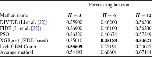
RMSSE results of the combination approaches

Table 1 Long description

A table comparing RMSSE results of different combination approaches across various forecasting horizons. The table has 6 rows and 4 columns. The columns are labeled as Method name, H = 3, H = 6, and H = 12. The rows are labeled with different methods: DIVIDE, FIDE, PSO, XGBoost (FIDE-based), LightGBM Comb, and Average method. Row 1: DIVIDE, 0.35900, 0.46200, 0.56300. Row 2: FIDE, 0.36900, 0.46100, 0.56200. Row 3: PSO, 0.36320, 0.46674, 0.57249. Row 4: XGBoost (FIDE-based), 0.35610, 0.45188, 0.54621. Row 5: LightGBM Comb, 0.35609, 0.45191, 0.54645. Row 6: Average method, 0.54193, 0.60601, 0.67144.

Table 2.

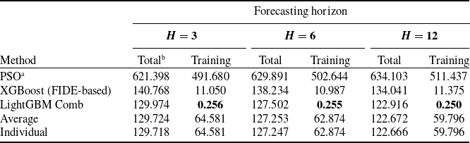
Run-time comparisons of the combination approaches

Table 2 Long description

A table comparing run-time of combination approaches for different forecasting horizons. The table has 5 rows and 7 columns. The columns are labeled as Method, Total for H = 3, Training for H = 3, Total for H = 6, Training for H = 6, Total for H = 12, and Training for H = 12. The rows are labeled as PSO, XGBoost (FIDE-based), LightGBM Comb, Average, and Individual. Row 1: PSO, 621.398, 491.680, 629.891, 502.644, 634.103, 511.437. Row 2: XGBoost (FIDE-based), 140.768, 11.050, 138.234, 10.987, 134.041, 11.375. Row 3: LightGBM Comb, 129.974, 0.256, 127.502, 0.255, 122.916, 0.250. Row 4: Average, 129.724, 64.581, 127.253, 62.874, 122.672, 59.796. Row 5: Individual, 129.718, 64.581, 127.247, 62.874, 122.666, 59.796.

^a “Train” time here refers to the weights optimisation time.

^b All times are in minutes.

Table 3.

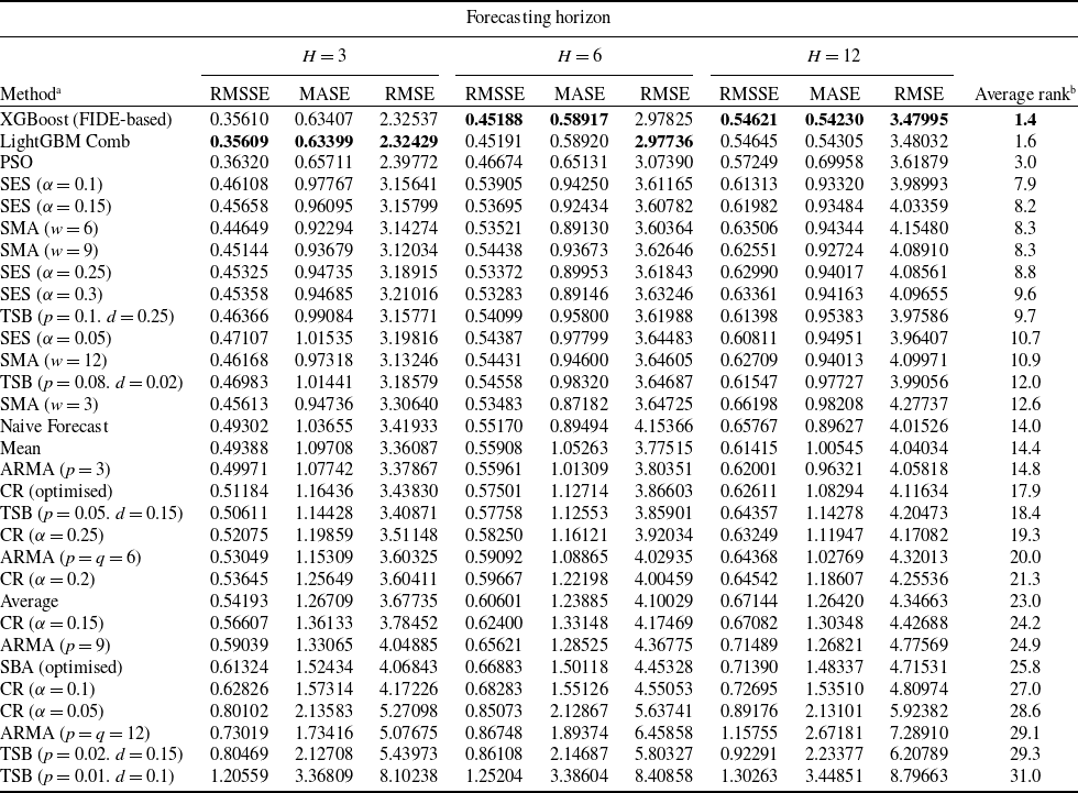
Accuracy results of individual and combination methods

Table 3 Long description

A table with 35 rows and 12 columns comparing the accuracy of individual and combination methods for forecasting horizons H = 3, H = 6, and H = 12. The columns are labeled RMSSE, MASE, RMSE for each horizon, and Average rank. The rows are labeled with different methods such as XGBoost, LightGBM Comb, PSO, SES, SMA, TSB, Naive Forecast, Mean, ARMA, CR, and SBA. Each row contains values for RMSSE, MASE, RMSE for each horizon, and the average rank. Notable trends include the methods XGBoost and LightGBM Comb having the lowest average ranks, indicating higher accuracy.

^a The parentheses values have the main parameters of each method.

^b The sum of all the method (line) rank position (in each column) divided by the total of metrics evaluated (9).