Molecular kinetic modelling of nanoscale slip flow using a continuum approach

Baochao Shan; Peng Wang; Runxi Wang; Yonghao Zhang; Zhaoli Guo

doi:10.1017/jfm.2022.186

Molecular kinetic modelling of nanoscale slip flow using a continuum approach

Published online by Cambridge University Press: 23 March 2022

and

Baochao Shan: Affiliation:
State Key Laboratory of Coal Combustion, Huazhong University of Science and Technology, Wuhan 430074, PR China
Peng Wang: Affiliation:
State Key Laboratory of Coal Combustion, Huazhong University of Science and Technology, Wuhan 430074, PR China
Runxi Wang: Affiliation:
School of Engineering, The University of Edinburgh, Edinburgh EH9 3FB, UK
Yonghao Zhang*: Affiliation:
School of Engineering, The University of Edinburgh, Edinburgh EH9 3FB, UK
Zhaoli Guo*: Affiliation:
State Key Laboratory of Coal Combustion, Huazhong University of Science and Technology, Wuhan 430074, PR China
*: †Email addresses for correspondence: yonghao.zhang@ed.ac.uk; zlguo@hust.edu.cn
†Email addresses for correspondence: yonghao.zhang@ed.ac.uk; zlguo@hust.edu.cn

Article contents

Abstract
Introduction
Governing equation and molecular-scale slip
Slip mechanisms and molecular kinetic modelling
Results and discussion
Conclusions
References

Rights & Permissions

Abstract

One major challenge for a continuum model to describe nanoscale confined fluid flows is the lack of a boundary condition that can capture molecular-scale slip behaviours. In this work, we propose a molecular-kinetic boundary condition to model the fluid–surface and fluid–fluid molecular interactions using the Lennard–Jones type potentials, and add a mean-field force to the momentum equation. This new boundary condition is then applied to investigate the nanoscale Couette and Poiseuille flows using the generalised hydrodynamic model developed by Guo et al. (Phys. Fluids, volume 18, issue 6, 2006a, 067107). The accuracy of our model is validated by molecular dynamics simulations and other models for a broad range of parameters including density, shear rate, wettability and channel width. Our simulation results reveal some unexpected and unintuitive slip behaviours at the nanoscale, including the epitaxial layering structure of fluids and the slip length minimum. The slip length minimum, which is analogous to the Knudsen minimum, can be explained by competing fluid–solid and fluid–fluid molecular interactions as density varies. A new scaling law is proposed for the slip length to account for not only the competing effect between the fluid–solid and fluid–fluid molecular interactions, but also many other physical mechanisms including the competition between the fluid internal potential energy and kinetic energy, and the confinement effect. While the slip length is nearly constant at the low shear rates, it increases rapidly at the high shear rates due to friction reduction. These molecular-scale slip behaviours are caused by energy corrugations at the fluid–solid interface where strong fluid–solid and fluid–fluid molecular interactions interplay.

JFM classification

Rarefied Gas Flow: Kinetic theory Rarefied Gas Flow: Molecular dynamics

Information

Type: JFM Papers
Information: Journal of Fluid Mechanics , Volume 939 , 25 May 2022, A9
DOI: https://doi.org/10.1017/jfm.2022.186 [Opens in a new window]
Copyright: © The Author(s), 2022. Published by Cambridge University Press

1. Introduction

Although the no-slip boundary condition is widely adopted in continuum fluid dynamics, it fails to account for the unexpected fast mass transport of fluids in the nanoscale systems (Holt et al. Reference Holt, Park, Wang, Stadermann, Artyukhin, Grigoropoulos, Noy and Bakajin2006; Falk et al. Reference Falk, Sedlmeier, Joly, Netz and Bocquet2010; Secchi et al. Reference Secchi, Marbach, Nigues, Stein, Siria and Bocquet2016), and may even lead to unrealistic simulated flow behaviours in, e.g. a liquid spreading on a solid substrate, corner flows, and extrusion of polymer melts from a capillary tube (Thompson & Troian Reference Thompson and Troian1997). In recent years, the rapid development of microtechnologies, nanotechnologies and related industrial processes including shale gas extraction, gas separation, self-cleaning surfaces, and tribology and lubrication (Urbakh et al. Reference Urbakh, Klafter, Gourdon and Israelachvili2004; Sholl & Johnson Reference Sholl and Johnson2006; Ma et al. Reference Ma, Gaisinskaya-Kipnis, Kampf and Klein2015; Yao et al. Reference Yao, Sanjayan, Song, Crick, Carmalt and Parkin2015; Wu et al. Reference Wu, Liu, Reese and Zhang2016; Cai et al. Reference Cai, Zhang, Wei, Guo, Li and Zhao2019; Ho et al. Reference Ho, Zhu, Wu, Wang, Guo, Ma and Zhang2019a) poses a research challenge in understanding and quantifying fluid slip dynamics at a fluid–solid interface, which may help to develop energy-efficient transportation with significant drag reduction (Martini et al. Reference Martini, Hsu, Patankar and Lichter2008a).

Slip dynamics of fluids over a solid surface has been extensively studied experimentally (Zhu & Granick Reference Zhu and Granick2001; Secchi et al. Reference Secchi, Marbach, Nigues, Stein, Siria and Bocquet2016; Henot et al. Reference Henot, Grzelka, Zhang, Mariot, Antoniuk, Drockenmuller, Leger and Restagno2018), theoretically (Richardson Reference Richardson1973; Lauga & Stone Reference Lauga and Stone2003; Nott Reference Nott2011; Wu et al. Reference Wu, Chen, Li, Li, Xu and Dong2017; Zampogna, Magnaudet & Bottaro Reference Zampogna, Magnaudet and Bottaro2018; Wang & Hadjiconstantinou Reference Wang and Hadjiconstantinou2019) and numerically (Thompson & Troian Reference Thompson and Troian1997; Sholl & Johnson Reference Sholl and Johnson2006; Martini et al. Reference Martini, Hsu, Patankar and Lichter2008a,Reference Martini, Roxin, Snurr, Wang and Lichterb; Falk et al. Reference Falk, Sedlmeier, Joly, Netz and Bocquet2010; Bailey, Hibberd & Power Reference Bailey, Hibberd and Power2017; Ho et al. Reference Ho, Li, Su, Wu, Borg, Li and Zhang2020). Due to difficulties and limitations of experimental and theoretical studies, molecular dynamics (MD) simulations have been widely adopted to probe the microscopic slip behaviours of fluids at the fluid–solid interface (Thompson & Troian Reference Thompson and Troian1997; Hsu & Patankar Reference Hsu and Patankar2010). Molecular dynamics results show that the surface effect is prominent in nanofluidics, and molecular-scale slip behaviours are greatly affected by the wall molecular potentials (Guo, Zhao & Shi Reference Guo, Zhao and Shi2006a; Mashayak & Aluru Reference Mashayak and Aluru2012), the cross-sectional fluid density and viscosity oscillations (Bhadauria, Sanghi & Aluru Reference Bhadauria, Sanghi and Aluru2015; Heiranian & Aluru Reference Heiranian and Aluru2020) and the fluid molecular interactions (Thompson & Troian Reference Thompson and Troian1997; Martini et al. Reference Martini, Hsu, Patankar and Lichter2008a,Reference Martini, Roxin, Snurr, Wang and Lichterb; Ho et al. Reference Ho, Papavassiliou, Lee and Striolo2011; Bitrián & Principe Reference Bitrián and Principe2018). These valuable insights help us to understand the mechanisms of molecular-scale slips at a fluid–solid interface from the molecular perspective. Due to the computational cost, MD simulations are restricted to extremely small systems and time steps, which have motivated researchers to develop computationally more efficient methods, e.g. continuum models. However, to date, it remains an open question on how to capture these molecular characteristics in a continuum modelling framework.

The difficulties of a continuum model in reproducing molecular-scale slip behaviours are mainly caused by inhomogeneities of the fluids with a vast fluid/surface region in nanoscale systems (Richardson Reference Richardson1973; Hocking Reference Hocking1976; Priezjev & Troian Reference Priezjev and Troian2006), where the fluid properties and its dynamical behaviour are significantly different from the bulk region (Sochi Reference Sochi2011; Guo et al. Reference Guo, Zhao and Shi2006a; Mashayak & Aluru Reference Mashayak and Aluru2012; Bhadauria et al. Reference Bhadauria, Sanghi and Aluru2015). For example, the epitaxial layering structure of fluids near the wall surface of a nano-confined system is associated with the molecular-scale slip at the fluid–solid interface (Voronov, Papavassiliou & Lee Reference Voronov, Papavassiliou and Lee2008), which can dramatically change the momentum transfer efficiency between the fluid and solid surface (Cao, Chen & Guo Reference Cao, Chen and Guo2006). Consequently, in order to reproduce molecular-scale slip behaviours by a continuum model, it is imperative to take these molecular-scale characteristics into account in a continuum modelling approach (Hsu & Patankar Reference Hsu and Patankar2010; Bhadauria et al. Reference Bhadauria, Sanghi and Aluru2015; Heiranian & Aluru Reference Heiranian and Aluru2020).

In recent years, some attempts have been made to develop continuum models to investigate molecular-scale slip behaviours in a nanoscale system (Hsu & Patankar Reference Hsu and Patankar2010) where the continuum fluid mechanics meets the molecular nature of matters (Secchi et al. Reference Secchi, Marbach, Nigues, Stein, Siria and Bocquet2016). For example, Hsu & Patankar (Reference Hsu and Patankar2010) studied the molecular-scale slip behaviours in nanochannels, which indicates that the continuum approach can describe molecular-scale slip behaviours provided underlying molecular-scale physics can be properly considered. According to Hsu & Patankar (Reference Hsu and Patankar2010), the following two challenges remain to be tackled.

(i) An effective solid–fluid potential, consistent with MD simulations, is needed to accurately describe surface fluid interactions.
(ii) The molecular interaction between fluid molecules requires us to consider the non-ideal gas effect in a dense fluid.

The generalised hydrodynamic model developed previously by one of the authors has partly addressed the second challenge (Guo et al. Reference Guo, Zhao and Shi2006a), where the Enskog equation for dense gases was used to take account of the non-ideal gas effect, and considered the surface–fluid interactions through the Lennard–Jones (LJ) type potentials, which has shown to be able to predict fluid layering structure in nano-confined spaces (Guo et al. Reference Guo, Zhao, Xu and Shi2006b; Shan et al. Reference Shan, Wang, Zhang and Guo2020). While these works indicate the feasibility of the continuum approach, the molecular-scale slip behaviours at the surface are not encapsulated, which will be addressed in the present work.

Molecular kinetic theory (MKT) has been proved to be effective in modelling chemical reactions (Glasstone, Laidler & Eyring Reference Glasstone, Laidler and Eyring1941), viscous flow (Martini et al. Reference Martini, Hsu, Patankar and Lichter2008a; Wang & Zhao Reference Wang and Zhao2011; Wang & Hadjiconstantinou Reference Wang and Hadjiconstantinou2019) and wetting dynamics (De Coninck & Blake Reference De Coninck and Blake2008; Yuan & Zhao Reference Yuan and Zhao2013), which bridges the molecular and continuum scales. While progress has been made to understand slip dynamics at the nanoscale, the underlying slip mechanisms are not fully understood. A slip model for a predictive simulation tool which encapsulates essential slip physics in particular fluid molecular interaction is still lacking (Wang & Hadjiconstantinou Reference Wang and Hadjiconstantinou2019).

Here, a new MKT slip model will be developed to consider the effect of molecular interactions between the fluid molecules and between the fluid and solid molecules on slip dynamics at the nanoscale. Together with the generalised hydrodynamic model (Guo et al. Reference Guo, Zhao and Shi2006a), the fluid dynamics at the nanometre scale can be described by a continuum approach. In § 2, a brief introduction to the generalised hydrodynamic model and slip dynamics at the nanoscale is given. In § 3, the molecular-scale slip dynamics in strongly inhomogeneous nanoscale system is discussed, leading to the new molecular-kinetic boundary condition. The simulation details and discussions are presented in § 4, and the conclusions are given in § 5.

2. Governing equation and molecular-scale slip

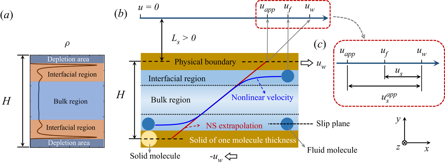
Here, we will use a continuum model to describe slip behaviour of fluid flows in confined nanoscale spaces. At the nanometre scale, the van der Waals forces between fluid molecules, and between fluid and solid molecules, become important, which are normally ignored in a continuum model. The fluid properties including density and viscosity oscillate significantly over a molecule size due to the fluid–solid and fluid–fluid molecular interactions (Bitsanis et al. Reference Bitsanis, Vanderlick, Tirrell and Davis1988; Bhadauria et al. Reference Bhadauria, Sanghi and Aluru2015; Heiranian & Aluru Reference Heiranian and Aluru2020). Therefore, such a system at the nanoscale is strongly inhomogeneous (Davis Reference Davis1987; Bitsanis et al. Reference Bitsanis, Vanderlick, Tirrell and Davis1988; Vanderlick, Scriven & Davis Reference Vanderlick, Scriven and Davis1989; Pozhar & Gubbins Reference Pozhar and Gubbins1993; Guo et al. Reference Guo, Zhao, Xu and Shi2006b; Dalton et al. Reference Dalton, Glavatskiy, Daivis and Todd2015; Shan et al. Reference Shan, Wang, Zhang and Guo2020). As shown in figure 1($a$,$b$), a depletion area exists in the immediate vicinity of the wall due to the volume exclusion effect or the short-range repulsion between solid and fluid molecules, which leads to difference between the physical boundary and the slip plane (Bhadauria et al. Reference Bhadauria, Sanghi and Aluru2015).

Figure 1.

Schematic of a nanoscale Couette flow and illustration of molecular-scale slip at the surface: ($a$) division of flow regions according to the density distribution; ($b$) the true and extrapolated velocity of a Couette flow; ($c$) the relationship between the micro and apparent velocities.

According to the fluid density distribution across the channel, the fluid can be divided into an interfacial region near the wall and a bulk region in the centre as shown in figure 1($a$). The interfacial region arises due to competing solid–fluid and fluid molecular interactions, exhibiting a layering structure near the wall (Patashinski et al. Reference Patashinski, Ratner, Orlik and Mitus2019; Kavokine, Netz & Bocquet Reference Kavokine, Netz and Bocquet2021). Consequently, the interfacial region is also called the gas adsorption area or adsorption layers, where the fluid density is normally larger than bulk density due to usually strong solid–fluid molecular attractions near the wall. In the bulk region, fluid molecules would not be affected by the wall potential, so the fluid density is constant.

Generally, the conventional Navier–Stokes (NS) equation, which describes fluid flows in a homogeneous system, will not be applicable to the interfacial region of strongly inhomogeneous fluids. In this work, we attempt to model nanoscale flows using a continuum approach, focusing on simple fluids.

2.1. Generalised hydrodynamic model

To reproduce molecular-scale slip behaviours by a continuum model, the fluid–solid and fluid molecular interactions should be appropriately taken into account (Hsu & Patankar Reference Hsu and Patankar2010). As an extension of the NS equation, a generalised hydrodynamic model was proposed by Guo et al. (Reference Guo, Zhao and Shi2006a) based on gas kinetic theory, which is applicable to both homogeneous and inhomogeneous systems. The mass and momentum conservation equations in this generalised hydrodynamic model can be written as

(2.1a)

\begin{gather} \partial_t \rho + \boldsymbol{\nabla} \boldsymbol{\cdot} (\rho \boldsymbol u)=0, \end{gather}

(2.1b)

\begin{gather}\partial_t (\rho \boldsymbol u) + \boldsymbol{\nabla} \boldsymbol{\cdot} (\rho \boldsymbol u \boldsymbol u)+ RT\boldsymbol{\nabla} \rho + \frac{\rho}{m}[\boldsymbol{\nabla} (\phi_w + \phi_m)-\boldsymbol G]= \boldsymbol{\nabla} \boldsymbol{\cdot} \left(\eta \widetilde{\boldsymbol{\nabla} \boldsymbol u} \right)\nonumber\\ \quad -\rho RT\left(2\boldsymbol A \chi + \boldsymbol B \bar{n} \right) V_0, \end{gather}

where $\rho = mn$ is the fluid density with $m$ being the mass of a fluid molecule and $n$ being the fluid number density, i.e. the fluid molecule numbers per unit volume; $u$, the fluid velocity; $t$, the time; $\phi _w$ and $\phi _m$, the wall potential and the fluid potential related to intermolecular attractions, respectively; $\boldsymbol G$, the body force; $\eta$, the fluid viscosity; $R=k_B/m$, the specific gas constant with $k_B$ being the Boltzmann constant; $T$, the fluid temperature; $\chi$, the radial distribution function; $V_0=2{\rm \pi} \sigma ^3/3$; $\bar {n}$, the local average density (Bitsanis et al. Reference Bitsanis, Magda, Tirrell and Davis1987); $\widetilde {\boldsymbol {\nabla } \boldsymbol u} = \boldsymbol {\nabla } \boldsymbol u + (\boldsymbol {\nabla } \boldsymbol u)^\intercal$; and $\boldsymbol A$ and $\boldsymbol B$, the two vector functions defined by (Guo, Zhao & Shi Reference Guo, Zhao and Shi2005)

(2.2a)

\begin{gather} \boldsymbol A(\boldsymbol r) = \frac{1}{D}\int_{|\boldsymbol r'|<\sigma/2} \boldsymbol r' \bar{n}(\boldsymbol r+\boldsymbol r')\,\mathrm{d}\boldsymbol r', \end{gather}

(2.2b)

\begin{gather}\boldsymbol B(\boldsymbol r) = \frac{1}{D}\int_{|\boldsymbol r'|<\sigma/2} \boldsymbol r' \chi[\bar{n}(\boldsymbol r+\boldsymbol r')]\,\mathrm{d}\boldsymbol r', \end{gather}

where $D={\rm \pi} \sigma ^5/120$ with $\sigma$ being the fluid molecule diameter; and $\boldsymbol r$ is the spatial position.

According to the Enskog theory for dense fluids (Chapman & Cowling Reference Chapman and Cowling1970), fluid viscosity needs to be corrected for dense fluids as fluid molecule size is not negligible and collisional transfer of momentum and energy needs to be considered, which can be evaluated by

(2.3)

\begin{equation} \eta = \eta_0 \bar{n} V_0 [(\bar{n}_f V_0 \chi)^{{-}1} + 0.8 + 0.7614 \bar{n} V_0 \chi], \end{equation}

where $\eta _0$ is the fluid viscosity for a dilute gas.

For a two-dimensional flow as shown in figure 1($b$), (2.1$b$) in the $y$-direction reduces to

(2.4)

\begin{equation} \frac{{\rm d}}{{\rm d} y}\left(\ln n + \frac{\phi_w + \phi_m}{k_B T}\right) ={-}(2A\chi+B\bar{n})V_0, \end{equation}

from which the density distribution across the channel can be obtained.

For Couette and Poiseuille flows, the velocity component in the $x$-direction can be determined by

(2.5)

\begin{equation} \frac{{\rm d}}{{\rm d} y}\left(\eta \frac{{\rm d}u}{{\rm d} y}\right) = 0 \end{equation}

and

(2.6)

\begin{equation} \frac{{\rm d}}{{\rm d} y}\left(\eta \frac{{\rm d}u}{{\rm d} y}\right) + G_x n = 0, \end{equation}

respectively, with $G_x$ in (2.6) being a constant external force in the flow direction.

As we can see from (2.4), (2.5) and (2.6), both density and velocity profiles are position dependent in nano-confined channels due to the effects of wall potential and fluid molecular interactions. This position dependence of fluid properties leads to some interesting and unexpected flow behaviours. However, in order to solve (2.5) and (2.6), appropriate boundary conditions, which are currently lacking, need to be specified.

2.2. Molecular scale slip

As discussed above, some unique features exist in strongly inhomogeneous fluid flows: (i) there is an interfacial region (also called an adsorption layer) near the wall, where the fluid density is much higher than in the bulk region, while the cross-sectional density is uniform in a conventional homogeneous system; (ii) in addition to the density and viscosity oscillations, the shear rate of a Couette flow is no longer constant and the velocity distribution is not linear, see figure 1. Similarly, the shear rate in a Poiseuille flow is no longer linear, with the velocity distribution being non-parabola; (iii) due to the finite size of fluid and solid molecules, and the strong repulsion between them when they are close, the first fluid layer is away from the physical boundary, i.e. the solid surface, which is illustrated by the dashed lines in figure 1($b$). These molecular features affect dynamics of strongly inhomogeneous fluid including both the velocity slip at the fluid–solid interface and the velocity distribution across the channel.

The slip phenomenon is generally quantified by the slip length $L_s$ (Thompson & Troian Reference Thompson and Troian1997; Martini et al. Reference Martini, Hsu, Patankar and Lichter2008a; Hsu & Patankar Reference Hsu and Patankar2010; Wang & Hadjiconstantinou Reference Wang and Hadjiconstantinou2019), which can be calculated according to the Navier slip boundary condition

(2.7)

\begin{equation} L_s = \frac{u_s^{app}}{\gamma}, \end{equation}

where $u_s^{app}$ is the apparent slip velocity as shown in figure 1($c$), and $\gamma$ is the shear rate evaluated in the bulk region. That is to say, the slip length in (2.7) is associated with the bulk region properties, where the NS equation is assumed to be valid. As shown in figure 1($b$), a slip length is positive when the extrapolated position, where the extrapolated velocity becomes equal to the wall velocity, is outside the physical boundary. The slip is also called a positive slip, otherwise, it is a negative or stick slip. Not only does the velocity distribution depend on fluid information in the bulk region (e.g. viscosity), but also the molecular interactions in the interfacial region (e.g. the fluid layering structure).

Taking a Couette flow as an example, in order to obtain the velocity distribution across the whole channel which is nonlinear as shown in figure 1($b$), the fluid velocity at the boundary needs to be determined. For strongly inhomogeneous nanoscale flows, a velocity difference exists between the wall and the fluid at the wall due to slip, which is called the micro slip velocity $u_s = |u_w - u_f|$, as shown in figure 1($c$). While the apparent slip velocity $u_s^{app}$ can be close to the true slip velocity $u_s$ when the interfacial region is negligible, their difference can be significant when the characteristic length of the flow domain reduces to the nanoscale. Therefore, we need to determine the true slip velocity $u_s$ to obtain the velocity distribution of strongly inhomogeneous flows.

3. Slip mechanisms and molecular kinetic modelling

In the previous slip models that are based on MKT, the slip resistance is usually considered to be caused by the fluid–solid molecular interaction only, e.g. (Glasstone et al. Reference Glasstone, Laidler and Eyring1941; Wang & Zhao Reference Wang and Zhao2011). However, fluid molecular interaction was found to contribute to slip resistance in nanoscale flows, which should be considered properly in an MKT slip model (Wang & Hadjiconstantinou Reference Wang and Hadjiconstantinou2019).

3.1. Slip mechanisms and related models

The slip dynamics of strongly inhomogeneous flows at the solid–liquid interface can be modelled as a thermally activated process (Glasstone et al. Reference Glasstone, Laidler and Eyring1941; Lichter et al. Reference Lichter, Martini, Snurr and Wang2007; Wang & Zhao Reference Wang and Zhao2011; Wang & Hadjiconstantinou Reference Wang and Hadjiconstantinou2019). Two key factors in MKT are the hopping length $\delta$ and the hopping rate $\alpha$. At equilibrium, fluid molecules preferentially occupy the most stable vacancies in energy corrugations. The hopping rates for the fluid molecules to move forwards and backwards are equal, which follows Arrhenius dynamics (Glasstone et al. Reference Glasstone, Laidler and Eyring1941; Martini et al. Reference Martini, Roxin, Snurr, Wang and Lichter2008b) as

(3.1)

\begin{equation} \alpha_+= \alpha_-= \alpha_0 =\frac{k_B T}{h}{\exp \left(-\frac{\Delta E}{k_B T}\right)}, \end{equation}

where $\alpha _+$, $\alpha _-$ and $\alpha _0$ are the hopping rates of moving forwards, backwards and at equilibrium, respectively; $h$ is the Planck constant; $\Delta E$ is the total energy barrier depth, which represents the total slip resistance from fluid–fluid and fluid–solid molecular interactions.

If a shear stress $\tau$ is exerted on fluid molecules in the flow direction, the energy of a fluid molecule to move forwards is elevated by the magnitude of $0.5\tau S \delta$, where $S$ is the effective area that the fluid molecule experiences the shear, so the probability of the fluid molecules moving forwards and backwards can be expressed by

(3.2a)

\begin{gather} \alpha_+=\frac{k_B T}{h}{\exp \left(-\frac{\Delta E-0.5\tau S \delta}{k_B T}\right)}, \end{gather}

(3.2b)

\begin{gather}\alpha_-=\frac{k_B T}{h} {\exp \left(-\frac{\Delta E+0.5\tau S \delta}{k_B T}\right)}. \end{gather}

The slip velocity $u_s=\delta (\alpha _+-\alpha _-)$ can consequently be calculated by

(3.3)

\begin{equation} u_s = \delta \frac{2k_B T}{h}{\exp \left(-\frac{\Delta E}{k_B T}\right)}{\sinh \left(\frac{\tau S \delta}{2k_B T} \right)}. \end{equation}

This is the classic MKT slip model proposed by Glasstone et al. (Reference Glasstone, Laidler and Eyring1941).

Based on the slip model (3.3), many other MKT models have been proposed to extend its applicability. Yang (Reference Yang2009) took the critical shear stress into account and proposed a new slip model. Similarly, Wang & Zhao (Reference Wang and Zhao2011) considered both the critical shear stress and the energy dissipation near the liquid–solid interface, and proposed the following extended MKT slip model:

(3.4)

\begin{equation} u_s = f_d\delta \frac{2k_B T}{h}\frac{F^+}{F_0}{\exp \left(-\frac{E_0}{k_B T}\right)}{\sinh \left[\frac{\text{Hev}(\tau-\tau_c) S \delta}{2k_B T} \right]}, \end{equation}

where $E_0$ is the activation energy at the absolute zero; $f_d$ is a dissipation factor, accounting for the energy dissipation between liquid layers at high shear stress, which is unity at low and moderate shear stress; $\text {Hev}()$ is the Heaviside function.

The critical shear stress $\tau _c$ was conjectured from experiments (Granick, Zhu & Lee Reference Granick, Zhu and Lee2003), but was found to be negligible in numerical simulations (Ma et al. Reference Ma, Shen, Sheridan, Liu, Chen and Zheng2011). In the linear flow regime, the energy dissipation factor $f_d$ may be neglected, so the slip model (3.4) reduces to (3.3). The above models (3.3) and (3.4) only consider the effect of fluid–solid molecular interaction on the slip resistance, and ignore the fluid molecular interaction.

3.2. Effect of fluid molecular interactions on slip dynamics

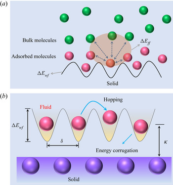
According to Blake & De Coninck (Reference Blake and De Coninck2002) and Zhao & Cheng (Reference Zhao and Cheng2017), the total resistance in a rate process arises from both fluid–solid and fluid–fluid molecular interactions, as shown in figure 2($a$). Assuming the superposition of the both potential contributions (Blake & De Coninck Reference Blake and De Coninck2002; Wang & Hadjiconstantinou Reference Wang and Hadjiconstantinou2019), i.e.

(3.5)

\begin{equation} \Delta E = \Delta E_{wf} + \Delta E_{ff}, \end{equation}

where $\Delta E_{wf}$ and $\Delta E_{ff}$ are the energy barrier depths related to fluid–solid and fluid–fluid molecular interactions, respectively, Wang & Hadjiconstantinou (Reference Wang and Hadjiconstantinou2019) proposed the following slip model:

(3.6)

\begin{equation} u_s = 2\delta \omega_0 \exp\left(-\frac{\Delta E_{wf}}{k_BT}\right) \sinh \left(\frac{S\delta}{2k_BT}\eta \gamma\right). \end{equation}

In (3.6), the shear stress $\tau$ in (3.3) is replaced by the product of viscosity $\eta$ and shear rate $\gamma$, which are evaluated at the interface between the interfacial and bulk regions. The slip length dependency on density, temperature and fluid–solid coupling strength has been fully investigated by Wang & Hadjiconstantinou (Reference Wang and Hadjiconstantinou2019). However, the parameter $\delta$ and the term $\omega _0 \exp {[-\Delta E_{wf}/(k_BT)]}$ are treated as fitting parameters which need to be calibrated for every operation condition by MD or experimental data. Therefore, this model provides a way to post-process MD or experimental data and does not have predictive power.

Figure 2.

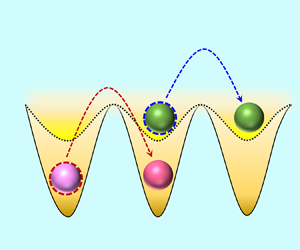
The schematic of fluid molecules passing over a solid surface. ($a$) The total resistance from the fluid–solid interaction $\Delta E_{wf}$ and fluid–fluid molecular interaction $\Delta E_{ff}$. ($b$) The lattice structure of a solid wall and the related energy corrugations over the surface.

3.3. Molecular kinetic modelling and analysis

Although the slip resistance arising from fluid molecular interactions should be considered, as pointed out by Wang & Hadjiconstantinou (Reference Wang and Hadjiconstantinou2019), how to quantify its effect on slip velocity remains unresolved. As shown in figure 2($a$), the resistance on a fluid molecule moving forwards originates from two components, namely the solid–liquid energy barrier $\Delta E_{wf}$ and the fluid–fluid energy barrier $\Delta E_{ff}$ (Blake & De Coninck Reference Blake and De Coninck2002; Zhao & Cheng Reference Zhao and Cheng2017; Wang & Hadjiconstantinou Reference Wang and Hadjiconstantinou2019). Here, we will develop our slip model through modelling of $\Delta E_{wf}$ and $\Delta E_{ff}$.

In our model, the molecular interactions between molecules are treated by the 12-6 LJ potential as in MD simulations (Thompson & Troian Reference Thompson and Troian1997; Martini et al. Reference Martini, Hsu, Patankar and Lichter2008a; Morciano et al. Reference Morciano, Fasano, Nold, Braga, Yatsyshin, Sibley, Goddard, Chiavazzo, Asinari and Kalliadasis2017), i.e.

(3.7)

\begin{equation} \phi_{ij} = 4 \epsilon_{ij}\left[\left(\frac{\sigma_{ij}}{r}\right)^{12} -\left(\frac{\sigma_{ij}}{r}\right)^6\right], \end{equation}

where $\epsilon _{ij}$ and $\sigma _{ij}$ are the energy and length parameters, $r$ is the distance between molecules and the subscripts $i$ and $j$ denote two interacting molecules. While the 12-6 LJ potential is widely adopted in MD simulations (Thompson & Troian Reference Thompson and Troian1997; Martini et al. Reference Martini, Hsu, Patankar and Lichter2008a,Reference Martini, Roxin, Snurr, Wang and Lichterb; Falk et al. Reference Falk, Sedlmeier, Joly, Netz and Bocquet2010; Bailey et al. Reference Bailey, Hibberd and Power2017; Morciano et al. Reference Morciano, Fasano, Nold, Braga, Yatsyshin, Sibley, Goddard, Chiavazzo, Asinari and Kalliadasis2017), it is seldom used in the mesoscopic kinetic and macroscopic continuum models (Mashayak & Aluru Reference Mashayak and Aluru2012; Bhadauria et al. Reference Bhadauria, Sanghi and Aluru2015; Shan et al. Reference Shan, Wang, Zhang and Guo2020). The effective radii of two different types of molecules is chosen at a position where repulsive interaction become pronounced. In addition, the energy parameter $\epsilon$ is related to the induced dipole interactions between two molecules. Therefore, the mixed energy and length parameters are determined by the Lorentz–Berthelot combination rule (Lorentz Reference Lorentz1881; Berthelot Reference Berthelot1898):

(3.8)

\begin{equation} \sigma_{ij} = \frac{\sigma_i + \sigma_j}{2}, \quad \epsilon_{ij} = \sqrt{\epsilon_i \epsilon_j}. \end{equation}

Considering the 12-6 LJ fluid–solid interactions and the lattice structure of the solids, the fluid–solid energy barrier $\Delta E_{wf}$ can be expressed as

(3.9)

\begin{equation} \Delta E_{wf} = a\epsilon_{wf}, \end{equation}

where $a$ is a constant characterising the strength of fluid–solid interactions. Although the relationship in (3.9) appeared in some studies (Wang & Zhao Reference Wang and Zhao2011; Wang & Hadjiconstantinou Reference Wang and Hadjiconstantinou2019), a full explanation of its physical meaning as well as its derivation is still missing. We include the detailed derivation and numerical validation in Appendix A.

Now we focus on modelling the effect of fluid molecular interaction on slip. The overall impact of surrounding fluid molecules on the slip of a molecule can be depicted by the term $\exp [-\Delta E_{ff}/(k_BT)]$ (Wang & Hadjiconstantinou Reference Wang and Hadjiconstantinou2019). However, an explicit determination of $\Delta E_{ff}$ is difficult (Wang & Hadjiconstantinou Reference Wang and Hadjiconstantinou2019). Since $\Delta E_{ff}$ is related to fluid molecules in both the interfacial and bulk regions, see figure 2($a$), we propose the following transformation:

(3.10)

\begin{equation} \frac{\Delta E_{ff}}{k_B T}\sim \frac{\epsilon_{wf}}{\epsilon_{ff}}. \end{equation}

It is noted that although the left-hand term in (3.10) explicitly includes temperature $T$, the term $\Delta E_{ff}/(k_B T)$ can be regarded as independent of $T$. For the physical process of molecular slip, an empty site will be available in the flow direction when a fluid molecule moves forward. According to Glasstone et al. (Reference Glasstone, Laidler and Eyring1941), the work required to make such an empty site is equal to the energy of vaporisation $\Delta E_{vap}$, which can relate to $\Delta E_{ff}$ as

(3.11)

\begin{equation} \Delta E_{vap}\sim \Delta E_{ff}. \end{equation}

As $\Delta E_{vap}/(k_BT) = b (v_m /v_f)^{1/3}$ (with $b$ being the packing number, $v_m$ being the molecular volume and $v_f$ being the molecular free volume; these parameters are negligibly affected by temperature) (Glasstone et al. Reference Glasstone, Laidler and Eyring1941; Blake & De Coninck Reference Blake and De Coninck2002), $\Delta E_{vap}/(k_BT)$ can be considered to be independent of temperature. Based on (3.11) and the physical process of molecular slip, (3.10) is a reasonable approximation to explicitly consider the effect of fluid molecular interaction on slip.

Considering both fluid–fluid and fluid–solid molecular interactions on slip, our MKT slip model can be written as

(3.12)

\begin{equation} u_s = f_{wet}\delta \frac{2k_B T}{h}{\exp \left(-\frac{a \epsilon_{wf}}{k_B T}\right)}{\sinh \left(\frac{\tau S \delta}{2k_B T} \right)}, \end{equation}

where $f_{wet}$ is a wettability factor accounting for fluid molecular interactions on slip, which can be expressed as

(3.13)

\begin{equation} f_{wet} =c_1\exp \left({-}c_2\frac{\epsilon_{wf}}{\epsilon_{ff}}\right), \end{equation}

where $c_1$ and $c_2$ are two fitting parameters depending on fluid and solid molecular properties.

Equation (3.12) is an extended MKT slip model, which bridges the molecular scale to the continuum hydrodynamics. Compared with the previous MKT slip models, all the parameters of our model are straightforward to determine, and do not depend on flow geometries or operation conditions. For example, $\delta$ is the distance between adjacent potential wells, which is related to the arrangement of solid molecules, see figure 2($b$); $S$ is the effective area, which can be taken as the square of the average distance between fluid molecules in the first adsorption layer; $f_{wet}$ needs to be calibrated once by MD simulation for a given fluid–solid system. Both fluid–solid and fluid molecular interactions on slip are considered. The fluid–solid energy barrier is modelled by (3.9), while the fluid–fluid energy barrier is modelled by the wettability factor $f_{wet}$ in (3.13). According to Barrat & Bocquet (Reference Barrat and Bocquet1999) and Śliwińska-Bartkowiak et al. (Reference Śliwińska-Bartkowiak, Sterczyńska, Long and Gubbins2014), the ratio $\epsilon _{wf}/\epsilon _{ff}$ is directly related to the wettability. This is physically reasonable since the distribution of fluid molecules under confinement is controlled by the wettability. The critical shear stress and the energy dissipation between adsorption layers are not taken into account in (3.12), but it is convenient to consider them if necessary as in Wang & Zhao (Reference Wang and Zhao2011). Since all parameters can be straightforwardly determined, this extended MKT slip model can be employed as a boundary condition for a continuum model to determine slip velocity at the fluid–solid interface, which will be elaborated in § 4.

It is noted that the slip velocity (3.12) models the hopping of molecules in the first adsorption layer, which corresponds to the surface diffusion rate of adsorbed gas (Ruckenstein & Rajora Reference Ruckenstein and Rajora1983; Shu, Teo & Chan Reference Shu, Teo and Chan2017). This is important in many engineering applications, such as shale gas and coal bed methane development, where adsorbed gas accounts for a large proportion in low-permeability shales and coals (Wu et al. Reference Wu, Tahmasebi, Lin, Zahid, Dong, Golab and Ren2019; Zhang et al. Reference Zhang, Shan, Zhao and Guo2019).

4. Results and discussion

Here, we apply the molecular-kinetic slip boundary condition (3.12) together with the generalised continuum model (2.4) and (2.5) to investigate nanoscale surface-confined Couette and Poiseuille flows. In Couette flows, the top and bottom plates move in the $x$ and $-x$ directions at a speed of $u_w$, while a constant external force $G_x$ is exerted on argon molecules in the $x$ direction in Poiseuille flows. The details of determining slip velocities and slip lengths in Couette and Poiseuille flows are introduced in Appendices B and C, respectively.

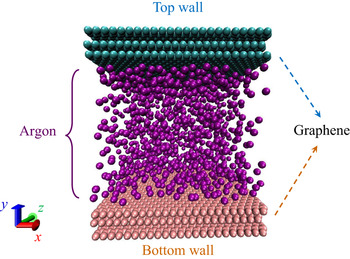
Meanwhile, MD simulations using LAMMPS (large-scale atomic/molecular massively parallel simulator) are conducted to validate the current continuum approach. In our non-equilibrium MD simulations, argon molecules are confined between two parallel graphite plates, as shown in figure 3. The 12-6 LJ potential is employed to model fluid–solid and fluid–fluid molecular interactions with a cutoff distance of 1.2 nm. The graphite molecules are fixed in our simulations. The system temperature is kept constant by implementing a Nosé–Hoover thermostat (Evans & Holian Reference Evans and Holian1985). The periodic boundary condition is employed in the $x$ and $z$ directions, respectively. After reaching equilibrium, the simulations are run with a time step of 2 fs for a minimum duration of 20 ns.

Figure 3.

Schematic of the physical model in MD simulations.

In our continuum and MD simulations of the nano-confined flows, we employ the same input parameters to ensure quantitatively meaningful comparisons. Unless otherwise specified, the corresponding parameters are: (i) the characteristic length of the flow path is $H = 5$ nm, which is the distance between the first layer of solid molecules in the top and bottom plates; (ii) an isothermal process with the system temperature of $T = 313$ K is considered; (iii) the average density of the fluids is controlled at $\rho = 500\,{\rm kg}\,{\rm m}^{-3}$; (iv) in the Couette flow, the top and bottom plates move with a speed of $u_w = 150\,{\rm m}\,{\rm s}^{-1}$ in the opposite directions; in the Poiseuille flow, the external force is set as $G_x = 0.0001\,{\rm kcal}\,(\,{\rm mol}\,{\rm A })^{-1}$; the plate velocity and the external force are chosen to ensure the flow in the linear flow regime, which means the slip length is not affected by the flow velocity; (v) the length and energy parameters of the solid and fluid as well as their masses are summarised in table 1.

Table 1.

Input parameters of argon (Barisik & Beskok Reference Barisik and Beskok2011) and graphene (Suk & Aluru Reference Suk and Aluru2017) for the continuum and MD simulations.

Here, we examine the role of temperature, characteristic length of the flow domain, wettability and density in slip dynamics. We also compare our slip model with the previous ones and establish a universal scaling law for the slip length.

4.1. The wettability factor accounting for fluid molecular interactions

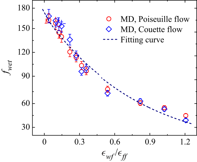
In the present slip model (3.12), the effect of fluid molecular interaction on slip is reflected by the wettability factor $f_{wet}$, which represents the resistance a fluid molecule ‘feels’ during slip exerted by its surrounding fluid molecules. By comparing slip velocities obtained from the slip model (3.12) and our MD simulations, the dependency of the wettability factor $f_{wet}$ on energy parameters ratio $\epsilon _{wf}/\epsilon _{ff}$ can be obtained, as shown in figure 4. Here, the fitting parameter is only calibrated once for the argon and graphene surface by the MD simulation in both Couette and Poiseuille flows. The calibrated relationship will then be used for all the other cases where the same argon and graphene are used in the following discussion.

Figure 4.

The dependency of wettability factor $f_{wet}$ on energy parameters ratio $\epsilon _{wf}/\epsilon _{ff}$. The fitting curve is (3.13) with $c_1=172.41$ and $c_2 = 1.28$.

The wettability factor $f_{wet}$ decreases rapidly with the energy parameters ratio $\epsilon _{wf}/\epsilon _{ff}$, indicating a larger fluid resistance on the slip of a molecule at stronger wettability conditions. As wettability increases, the fluid density becomes larger in the first adsorption layer, leaving fewer empty sites along the flow direction for an activated molecule to move forwards. Consequently, although the flow resistance from the bulk fluid becomes smaller, it is harder for a fluid molecule to slip. This also indicates that the flow resistance from the adsorbed fluid molecules is much larger than from the bulk ones.

4.2. Effect of temperature on slip length

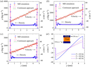
The density and velocity profiles of the argon between the moving graphite plates are displayed in figure 5 at $T = 253$ K, $T = 353$ K and $T = 453$ K, respectively. Here, to examine the effect of temperature, we keep all the parameters the same except for temperature. The effect of other parameters (width, wettability and density) is also analysed in this way in the following subsections.

Figure 5.

The comparison of cross-sectional density and velocity distributions between our continuum and MD simulations at ($a$) $T$ = 253 K, ($b$) $T$ = 353 K and ($c$) $T$ = 453 K, respectively; and ($d$) comparison of the velocity profiles obtained by the continuum model at different temperatures.

As shown in figure 5, a strong adsorption layer forms at the fluid–solid interface followed by a second layer of weak adsorption due to the competition between the fluid–solid and fluid–fluid molecular interactions. As previously reported (Voronov et al. Reference Voronov, Papavassiliou and Lee2008; Ho et al. Reference Ho, Papavassiliou, Lee and Striolo2011), these epitaxial layering structures in the vicinity of the solid surface dominate the slip dynamics at the fluid–solid interface at the nanoscale. Consequently, the boundary condition alone, no matter a hydrodynamic one or a molecular kinetic one, is not sufficient to describe the true slip dynamics, since the inhomogeneity of the fluid flow has to be considered by the governing equations (Hsu & Patankar Reference Hsu and Patankar2010). Moreover, fluid adsorption is important in many engineering applications, e.g. unconventional shale gas production (Germanou et al. Reference Germanou, Ho, Zhang and Wu2018; Zhang et al. Reference Zhang, Shan, Zhao and Guo2019). Therefore, the required large-scale engineering simulations motivate us to develop a computationally efficient model to capture molecular-scale interactions and to accurately predict hydrodynamic behaviour at the system scale (Ho et al. Reference Ho, Zhu, Wu, Wang, Guo, Li and Zhang2019b).

Figure 5 also shows good agreement between our continuum and MD simulations considering the influence of temperature on the velocity profiles. Furthermore, from figure 5($d$), we can see that the slip velocity increases with temperature, which is reasonable since the kinetic energy of the fluid molecules, which escape from the potential wells, is larger at a higher temperature. While the bulk fluid flow can be described by classical continuum models with slip boundary conditions, the detailed flow behaviour of gas adsorption is completely ignored. However, the nanoscale confinement effect is more than a slip velocity at the solid surface, because the thickness of adsorption layers may not be negligibly small compared with the flow dimension, which depends on the strength of interaction potentials between the surface and fluid molecules. Therefore, a slip velocity at the boundary is not sufficient to account for the nanoscale effect in an inhomogeneous system, which we would like to emphasise again.

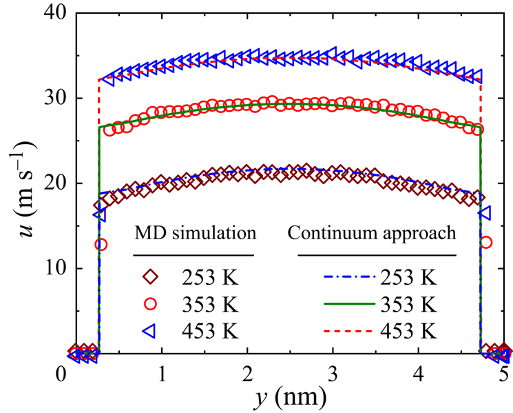
The effect of temperature on velocity profiles of Poiseuille flows is shown in figure 6. Again, a good agreement between the continuum and the MD results is observed at different temperatures. Due to the large slip velocity in nano-graphene channels, the velocity distribution is plug-like, significantly enhancing the mass transfer efficiency in such structures.

Figure 6.

The effect of temperature on the velocity profiles of the Poiseuille flows.

4.3. Effect of channel width on slip length

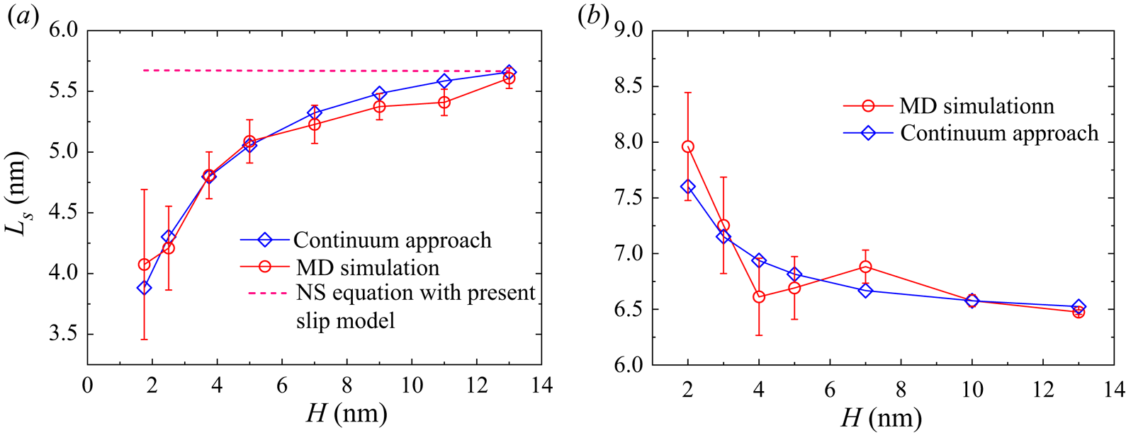
The effect of channel width $H$ on the slip length of Couette and Poiseuille flows is shown in figure 7 where $H$ ranges from 2.0 nm to 13.0 nm. Previously, it was reported that the slip length $L_s$ was independent of the channel width $H$ (Cieplak, Koplik & Banavar Reference Cieplak, Koplik and Banavar2001) where the range of channel width was not specified. However, as shown in figure 7($a$), the slip length does increase with the channel width rapidly in highly confined Couette flows, while it decreases with the channel width $H$ in Poiseuille flows. Keerthi et al. (Reference Keerthi2018) experimentally reported the helium transport driven by pressure through two-dimensional nanochannels for different wall materials and observed that the slip length decreases with the channel width, which is consistent with our computational finding. However, helium has a smaller mass and weaker interactions with surface molecules, and the experiment was conducted in an ultra-rarefied condition with Knudsen number $Kn>10^4$. Therefore, the observed enhancement effect in the experiment (Keerthi et al. Reference Keerthi2018) is more significant than our simulations of dense argon flows with $Kn$ close to $0.01$. For both Couette and Poiseuille flows, when $H$ becomes sufficiently large, the slip length plateaus, which is consistent with Kannam et al. (Reference Kannam, Todd, Hansen and Daivis2013).

Figure 7.

The effects of channel width $H$ on the slip length: ($a$) the Couette flow; and ($b$) the Poiseuille flow.

For comparison, the slip length obtained from the NS equation with the present slip model (3.12) is also included in figure 7, where the wettability factor is chosen to ensure the slip velocities for our continuum model and the NS equation are the same at $H=5$ nm. The parameters such as viscosity and the effective area are evaluated at the average density $\rho _{avg}=500\,{\rm kg}\,{\rm m}^{-3}$. The NS model predicts that slip length does not depend on channel width, which is different from the findings of our continuum and MD simulations. This further proves that a slip boundary condition alone cannot capture the slip dynamics accurately in small nanochannels, e.g. $H<13$ nm in this study.

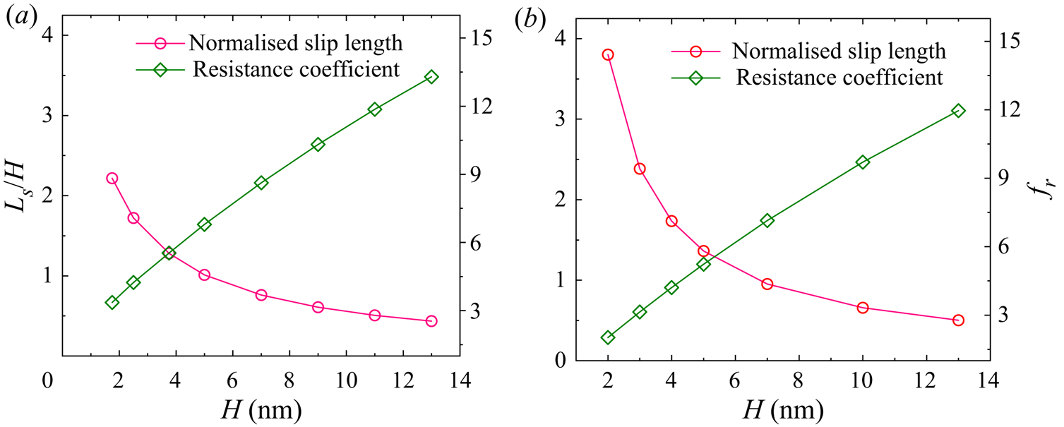
On the other hand, the normalised slip length, i.e. ratio of slip length to channel width $L_s/H$, decreases with the channel width in both Couette and Poiseuille flows, as shown in figure 8. According to Cao et al. (Reference Cao, Chen and Guo2006), the flow resistance coefficient can be calculated by

(4.1)

\begin{equation} f_r = \frac{48}{\mbox{{Re}}} \frac{1}{1 + 6 \frac{L_s}{H}}, \end{equation}

where $\mbox { {Re}}$ is the Reynolds number and $f_r$ is the resistance coefficient. As indicated by (4.1), the overall flow resistance is mainly controlled by the ratio $L_s/H$ at a fixed $Re$. Figure 8 shows how the resistance coefficient varies with channel widths at $\mbox { {Re}} = 1$. Clearly, the flow resistance is smaller in the narrower nanochannels due to the larger $L_s/H$, i.e. the slip reduces the flow resistance in highly confined nanochannels. Compared with a Couette flow, the flow resistance in a Poiseuille flow is smaller due to a larger slip length at narrow nanochannels. This indicates that the nano-confinement effect on the flow physics of Couette and Poiseuille flows is different.

Figure 8.

The effects of channel width $H$ on the normalised slip length and the resistance coefficient: ($a$) the Couette flow; and ($b$) the Poiseuille flow.

4.4. Effect of wettability on slip length

The fluid–surface molecular interactions are key to understanding slip flow behaviours at the nanoscale. One of the main differences of our continuum model from the previous ones is that the fluid–fluid and fluid–solid molecular interactions are considered exactly the same as those in MD simulations. Here, the effect of molecular interactions, as reflected by ratio of the fluid–solid energy parameter to the fluid–fluid energy parameter, i.e. $\epsilon _{wf}/\epsilon _{ff}$, is investigated.

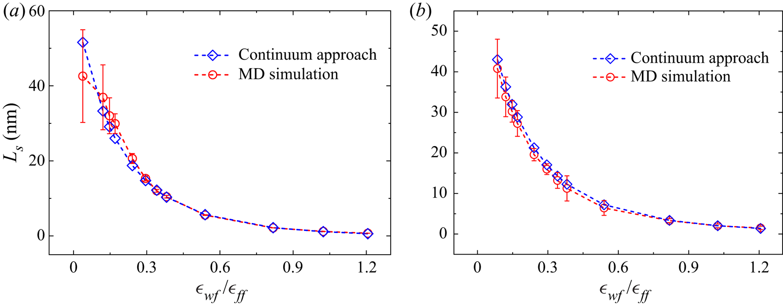
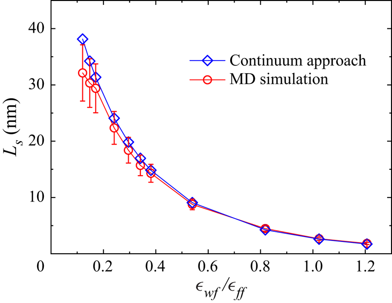
As shown in figure 9, the slip length decreases with $\epsilon _{wf}/\epsilon _{ff}$ via a power law relationship and tends to no-slip when this ratio is sufficiently large in both Couette and Poiseuille flows. Again, our continuum results agree well with the MD data. The strong interactions among fluid and solid molecules as well as the lack of empty sites along the flow direction resist the fluid molecules to slip over a solid substrate at larger $\epsilon _{wf}/\epsilon _{ff}$, while the solid surface becomes repulsive and the viscous resistance becomes smaller when the fluid–solid coupling becomes weaker, which prompts the fluid molecules to slip over the solid surface. This finding is also consistent with the results of previous MD simulations (Barrat & Bocquet Reference Barrat and Bocquet1999; Voronov, Papavassiliou & Lee Reference Voronov, Papavassiliou and Lee2006).

Figure 9.

A comparison of the slip length predicted by our continuum and MD simulations at different wettability conditions: ($a$) the Couette flow; and ($b$) the Poiseuille flow.

4.5. Effects of density on slip length

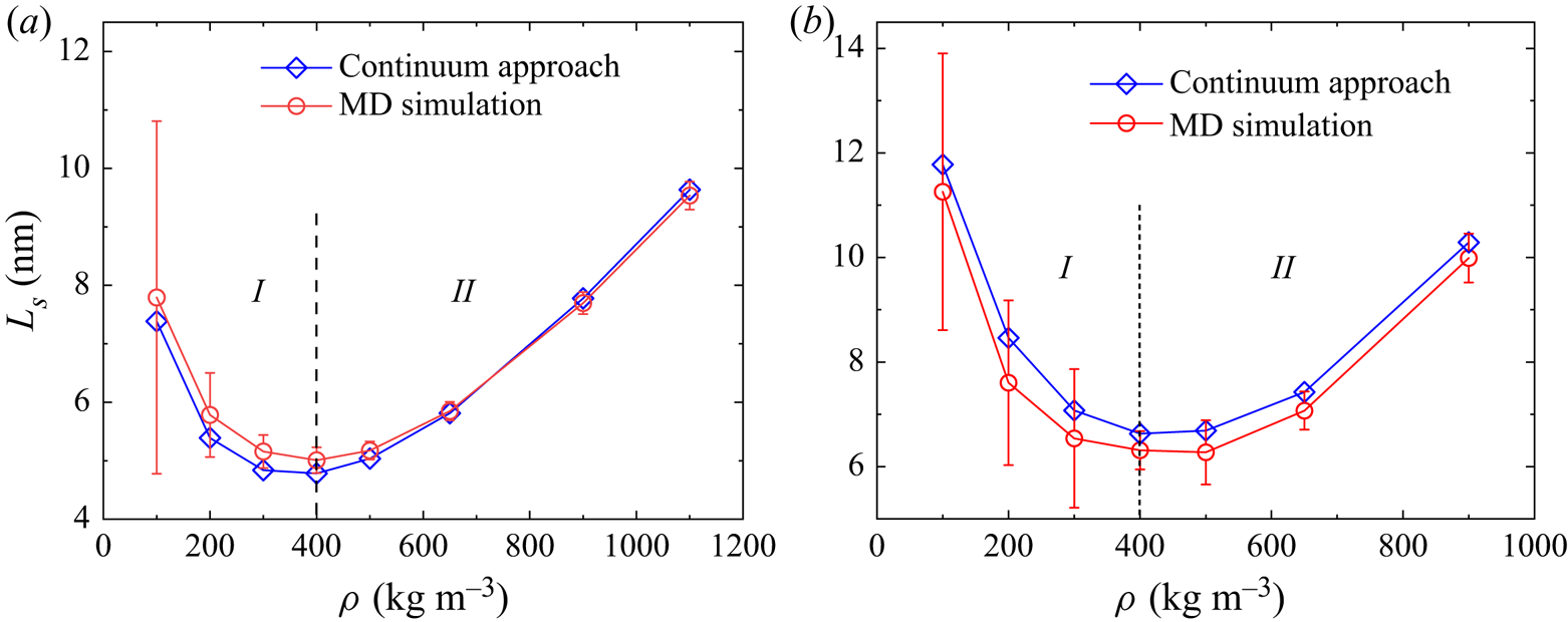
It was reported that the slip length decreases with fluid density in the MD simulations (Koplik, Banavar & Willemsen Reference Koplik, Banavar and Willemsen1989; Barrat & Bocquet Reference Barrat and Bocquet1999; Voronov et al. Reference Voronov, Papavassiliou and Lee2008), which is consistent with the kinetic theory for rarefied gas flows. However, it is shown by our continuum model that the slip length increases with density for large densities, as shown in figure 10.

Figure 10.

A comparison of the slip length dependence on density between the continuum and MD simulations: ($a$) the Couette flow; and ($b$) the Poiseuille flow.

We perform MD simulations for the Couette and Poiseuille flows to verify this new finding. Our results are shown in figure 10. In both types of flows, there are two distinct regimes, $I$ and $II$, divided by the critical density marked by the vertical dashed line at $\rho =400\,{\rm kg}\,{\rm m}^{-3}$. For a dense fluid flow, the $Kn$ is defined (Chapman & Cowling Reference Chapman and Cowling1970) as

(4.2)

\begin{equation} Kn = \frac{1}{\sqrt{2} n_{avg} {\rm \pi}\sigma^2 \chi H}, \end{equation}

where $n_{avg}$ is the average fluid number density. Using this definition, the Kn is approximately 0.046 in the system considered. Consequently, in regime $I$, namely for $\rho < 400\,{\rm kg}\,{\rm m}^{-3}$ (Kn $>$ 0.046), the rarefaction effect is important, where the fluid–solid molecular interaction dominates. In this regime, the slip length increases as density decreases, which is consistent with the gas kinetic theory (Koplik et al. Reference Koplik, Banavar and Willemsen1989; Barrat & Bocquet Reference Barrat and Bocquet1999; Voronov et al. Reference Voronov, Papavassiliou and Lee2008). In regime $II$ for $\rho > 400\,{\rm kg}\,{\rm m}^{-3}$ (Kn $<$ 0.046), the fluid becomes denser. In this regime, the average distance between fluid molecules is much smaller, and the fluid–fluid molecular interaction becomes non-negligible. The slip length in this regime is found to increase with the fluid density, which is contrary to the kinetic theory.

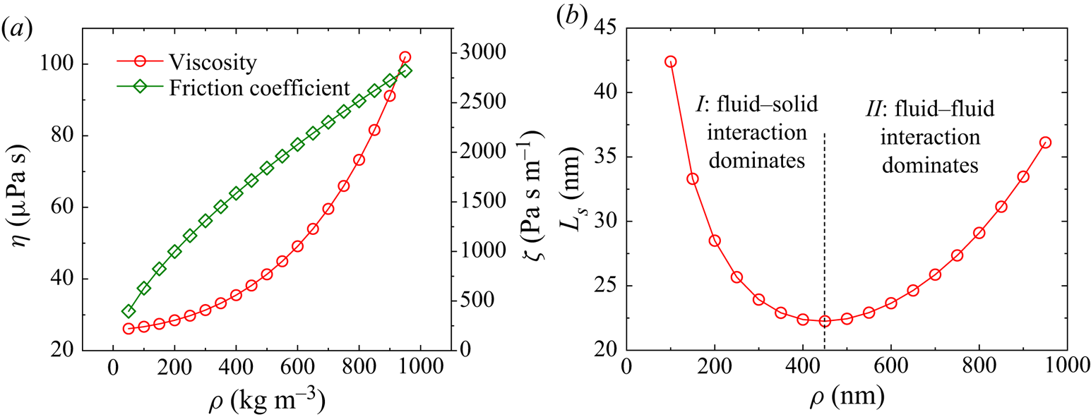
The above competing fluid–solid and fluid molecular interactions on the slip length $L_s$ can be intuitively explained by the definition of the slip length. In (2.7), the slip velocity can be expressed as $u_s=\tau /\zeta =\eta \gamma /\zeta$ with $\zeta$ being the friction coefficient between the fluid and solid, and the slip length can consequently be expressed by two properties of the fluid–solid system, namely

(4.3)

\begin{equation} L_s=\frac{\eta}{\zeta}. \end{equation}

At different densities, the fluid viscosity $\eta$ can be calculated by (2.3), while the friction coefficient $\zeta$ can be derived from the slip model (3.12), see Appendix D. The friction coefficient and viscosity can reflect the strength of fluid–solid and fluid–fluid molecular interactions, respectively. Although both parameters increase with density, the friction coefficient increases faster for small densities and more slowly for large densities, but the opposite is true for the viscosity, see figure 11. The competing effect between fluid–solid and fluid–fluid molecular interactions leads to a slip length minimum analogous to the Knudsen minimum phenomenon in rarefied gas dynamics as shown in figure 11($b$). So at small densities, the flow is dominated by fluid–solid interaction where the slip length decreases when the density increases; while at large densities, the flow is dominated by fluid molecular interactions where the slip length increases with density. Furthermore, the inflexion density is also at approximately $\rho =425\,{\rm kg}\,{\rm m}^{-3}$, which is close to the continuum and MD simulation results presented in figure 10, supporting our explanation of the physical mechanism underlying the slip length minimum. It is noted that the slip length shown in figure 11 is higher than our continuum and MD simulation results presented in figure 10. This discrepancy arises from the fact that the effective area $S$ in (D3) is evaluated using the average density, while the density of the adsorbed gas should be used since the slip occurs at the adsorption layer in the immediate contact with the wall. With this correction, the predicted slip lengths are consistent.

Figure 11.

($a$) The variation of viscosity and friction coefficient with density, and ($b$) the competing effect of the fluid–solid and fluid–fluid molecular interactions on slip length.

The slip length minimum can also explained from a force balance perspective. In a Couette flow, for example, it is the friction force that drives the fluid layer adjacent to the plates to move first, and the bulk fluid will resist this movement through the viscous shear force. In regime II, the fluid viscosity becomes large as density increases such that the friction force at the fluid–solid interface is not sufficient to overcome the viscous shear force in the central bulk region at a larger shear rate (i.e. a smaller slip length). Consequently, the shear rate will decrease to reduce the viscous shear force to establish a steady Couette flow, which explains the increasing slip length with density in this regime. This phenomenon can also be observed at different fluid–solid coupling strengths, as shown in figure 10($b$).

4.6. A scaling law for the slip length minimum

As we can see from figures 10 and 11($b$), regime $I$, where the fluid–solid interaction dominates the flow, transits to regime $II$, where the fluid molecular interaction is more important, at nearly the same inflection density. As discussed above, the non-monotonicity of the slip length dependency on density reflects the competition between the fluid–solid and fluid molecular interactions, which can be characterised by the friction coefficient and the viscosity, respectively. This slip length minimum is interestingly analogous to the Knudsen minimum (Sheng et al. Reference Sheng, Gibelli, Li, K Borg and Zhang2020).

Meanwhile, as indicated by the generalised hydrodynamic model (2.1) and (2.4), wall potential $\phi _w$ and fluid intermolecular potential $\phi _m$ as well as the system temperature $T$ play crucial roles in the strongly inhomogeneous systems. To quantify the effect of these factors, the parameter $\prod$ is devised as (Guo et al. Reference Guo, Zhao and Shi2006a)

(4.4)

\begin{equation} \prod = \frac{1}{H - 2\iota} \int_{\iota}^{H - \iota} \frac{\phi_w+\phi_m}{k_B T}{{\rm d} y}\approx \frac{\epsilon_{ff}}{k_B T}\left(b_1\frac{\sigma}{H}\frac{\epsilon_{wf}}{\epsilon_{ff}}+b_2 n_{avg}\sigma^3 \right), \end{equation}

where $\iota$ is the distance between the first fluid layer to the solid; and $b_1$ and $b_2$ are two constants related to the wall potential and the fluid intermolecular potential, respectively. Consequently, a typical nanoscale dense fluid system can be characterised by four non-dimensional parameters, i.e. the reduced temperature $T_r=k_BT/\epsilon _{ff}$, the confinement factor $H/\sigma$, the energy ratio $\epsilon _{wf}/\epsilon _{ff}$, and the reduced fluid density $n_{avg}\sigma ^3$.

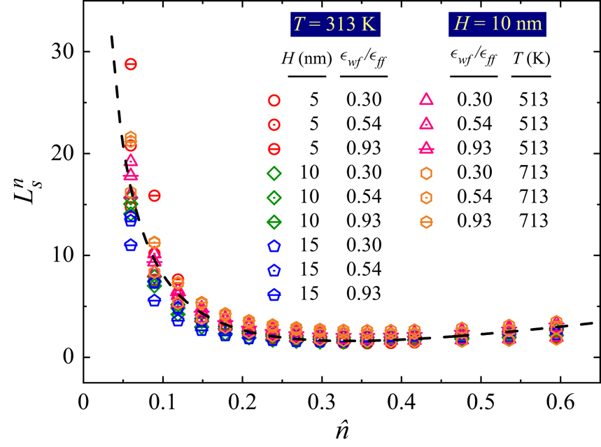
Inspired by (4.4), we propose the following universal scaling law for non-dimensional slip length as

(4.5)

\begin{equation} L_s^n = \frac{L_s}{\sigma} \frac{H}{\sigma} \left(\frac{\epsilon_{wf}}{\epsilon_{ff}}\right)^{\beta} \frac{\epsilon_{ff}}{k_B T} \frac{\eta}{\eta_{0}} Kn, \end{equation}

where $\beta$ is a constant for a given solid and fluid system. Here, the ratio $\epsilon _{wf}/\epsilon _{ff}$ reflects the competition between the fluid–wall and fluid molecular interactions, and the ratio $\epsilon _{ff}/(k_BT)$ gives the competition between the fluid internal potential energy and kinetic energy. The denseness effect is characterised by the viscosity ratio between the dense fluid and the corresponding dilute one, i.e. $\eta /\eta _0$, and the rarefaction effect is illustrated by the Knudsen number Kn. Using this scaling law, the relationship between the non-dimensional slip length $L_s^n$ and the reduced density $\hat {n}=n_{avg}\sigma ^3$ in different systems is shown in figure 12, where all the data almost collapse into a single line. This confirms our statement that the non-monotonicity of slip length on density is a result of the competition between the fluid–solid and fluid molecular interactions, analogous to the Knudsen minimum. At low densities, the slip length decreases when the density increases, while it increases with the density linearly at high densities, regardless of the fluid–solid coupling strength, the system temperature and dimension.

Figure 12.

A universal scaling law of slip length considering the effects of density, fluid–solid coupling strength, channel width and system temperature.

4.7. Slip length dependency on shear rate

The pioneering work of Thompson & Troian (Reference Thompson and Troian1997) reported that the Navier slip boundary condition is only applicable at low shear rates, and the slip length increases rapidly with $\gamma$ at high shear rates (Thompson & Troian Reference Thompson and Troian1997). Based on their MD simulation results, a general scaling law for the slip length was proposed as

(4.6)

\begin{equation} L_s = L_s^0(1-\varGamma)^{{-}0.5}, \end{equation}

where $L_s^0$ is the limiting slip length at low shear rates; $\varGamma$ is the ratio of the shear rate $\gamma$ to the critical shear rate $\gamma _c$.

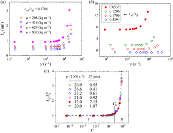
The present continuum model allows us to simulate a wide range of nanoscale confined flows with different densities, temperatures, fluid–solid coupling strengths, shear rates and flow geometries to check the validity of the above scaling law and to unravel the underlying mechanisms. Our simulation results are shown in figure 13. The slip length dependency on density and fluid–solid coupling strength can be clearly observed. The slip length is nearly constant at low shear rates and increases rapidly after the critical shear rate $\gamma _c$. The results also suggest that the critical shear rate is not affected by the density, but increases with the increasing fluid–solid coupling strength. It is noted that a stick slip, where the slip length is negative, is found at the strong fluid–solid coupling strength in figure 13($b$).

Figure 13.

Dependency of the slip length on ($a$) density, ($b$) fluid–solid coupling strength and ($c$) comparison between our continuum model (symbols) and the general scaling law (4.6) of Thompson & Troian (Reference Thompson and Troian1997) (dashed line).

In figure 13($c$), the dashed line is the result of the scaling law (4.6) obtained from the MD simulations (Thompson & Troian Reference Thompson and Troian1997), which is in excellent agreement with our results. As shown in figure 13($c$), two slip flow regimes are divided by the non-dimensional shear rate $\varGamma = \varGamma _0$ as indicated by the vertical dashed line. With $\varGamma <\varGamma _0$, it is the linear Navier slip flow regime (I), in which the slip length increases linearly with the shear rate, namely the so-called linear response regime. When $\varGamma >\varGamma _0$, the friction-reduction slip flow regime starts. In this regime (II), the friction coefficient decreases with the shear rate. Our continuum model is able to capture these unique molecular-scale slip characteristics, which further confirms the validity of our model. So the present continuum mode is well-suited for large-scale simulations beyond the reach of MD simulations.

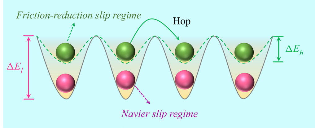
At a fluid–solid interface, the microscopic friction coefficient $\zeta$ is defined as the ratio of viscosity to slip length, namely (4.3). For Newtonian fluids, the viscosity $\eta$ is independent of shear rate (Thompson & Troian Reference Thompson and Troian1997). As the slip length increases, the friction coefficient decreases with the shear rate. This reduction of the friction coefficient can be explained by the landscape of energy corrugation. There are energy corrugations over the wall surface due to the lattice structure of solids, see figure 14. At a low shear rate, there is sufficient time for fluid molecules to occupy the low energy sites and remain in a stable state, as shown in figure 14 of the Navier slip flow regime. In this regime (I), the fluid molecules (in red) need to overcome $\Delta E_l$ to hop from one site to another. As the shear rate increases, the speed of fluid molecules at the interface also increases. When the fluid moves fast enough, fluid molecules do not invaginate themselves into the lower potential energy levels, but rather skim over the substrate (Martini et al. Reference Martini, Hsu, Patankar and Lichter2008a), exhibiting a smaller energy barrier depth $\Delta E_h$. When the shear rate, i.e. the fluid moving speed is sufficiently large, the energy barrier depth tends to zero, namely $\Delta E \rightarrow 0$. In this case, the solid–fluid interface becomes frictionless, and the slip tends to be infinite (Wu et al. Reference Wu, Chen, Li, Li, Xu and Dong2017), i.e. $L_s \to +\infty$.

Figure 14.

The fluid slip length at low and high shear rates.

4.8. Model analysis

Here, we apply the continuum model ((2.1) and (3.12)) to simulate the slip flows of $\rho = 800\,{\rm kg}\,{\rm m}^{-3}$, $T= 353$ K, $H= 6$ nm using the wettability factor $f_{wet}$ relationship in figure 4 which is calibrated at $\rho =500\,{\rm kg}\,{\rm m}^{-3}$, $T=313$ K and $H=5$ nm. The results of the slip flows over a wide range of fluid–solid coupling strengths are presented in figure 15. The corresponding MD simulations are also conducted which show good agreement with the continuum results, see figure 15. As the wettability weakens, the continuum results gradually deviate from the MD data. Considering the uncertainties in MD simulations and the large slip in the simulated system for low wettability, the relative difference is still not significant. Therefore, the new boundary condition (3.12) can help the present continuum model to accurately simulate slip flows, which is computationally efficient to enable practical engineering simulations. Even if the energy parameter of carbon molecules $\epsilon _w$ is changed, the boundary condition still holds as long as the array of surface molecules remain unchanged, which further indicates the applicability of the present continuum model for nanoscale confined flows.

Figure 15.

Using the continuum approach to simulate the slip flows of $\rho = 800\,{\rm kg}\,{\rm m}^{-3}$, $T= 353$ K, $H= 6$ nm over a wide range of fluid–solid coupling strengths.

4.9. A comparison with other slip models

The MKT slip model (3.4) proposed by Wang & Zhao (Reference Wang and Zhao2011) reduces to (3.3), which is proposed by Glasstone et al. (Reference Glasstone, Laidler and Eyring1941), if the shear stress is low and the critical shear stress is negligible. In our study, the simulated cases are in the linear flow regime and there is no critical shear stress observed. Therefore, we compare our model with the Glasstone MKT model described by (3.3). Meanwhile, the commonly employed second-order slip boundary condition for the NS equation is also included for comparison, which is

(4.7)

\begin{equation} u_s^{app}-u_w={\pm} C_1 \lambda \left(\frac{\partial u}{\partial n}\right)_s- C_2\lambda^2 \left(\frac{\partial^2 u}{\partial n^2}\right)_s, \end{equation}

where $C_1$ and $C_2$ are the first- and second-order slip coefficients, which are taken as $C_1=1.0$ and $C_2 = 0.5$ in our study (Chapman & Cowling Reference Chapman and Cowling1970). Combining the second-order slip boundary condition with the Stokes equation, the slip velocity can be calculated as

(4.8)

\begin{equation} u_s^{app} ={-}\frac{H^2}{2\eta}\frac{\mathrm{d}p}{\mathrm{d}\kern0.7pt x}(C_1 Kn+2C_2Kn^2). \end{equation}

Here, we note that only the apparent slip velocity can be calculated from the second-order slip boundary condition, while a micro slip velocity can only be calculated from MKT slip models.

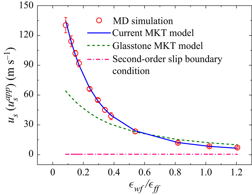
The comparisons of different models are shown in figure 16, where the MD data serve as the benchmark solution. The Glasstone model (3.3) fails to capture the slip dynamics for different wettability, while the results of the current model are in excellent agreement with the MD data. Since the $Kn$ is independent of the wettability, the slip velocity from the second-order slip boundary condition is constant, which is much smaller than the other predictions, especially for weak wettability. Therefore, the second-order slip boundary condition is not applicable for strongly inhomogeneous nanoscale flows.

Figure 16.

Model comparison for slip velocity under different wettability, where the MD results serve as the benchmark solution.

4.10. Navier–Stokes equation with the current slip model

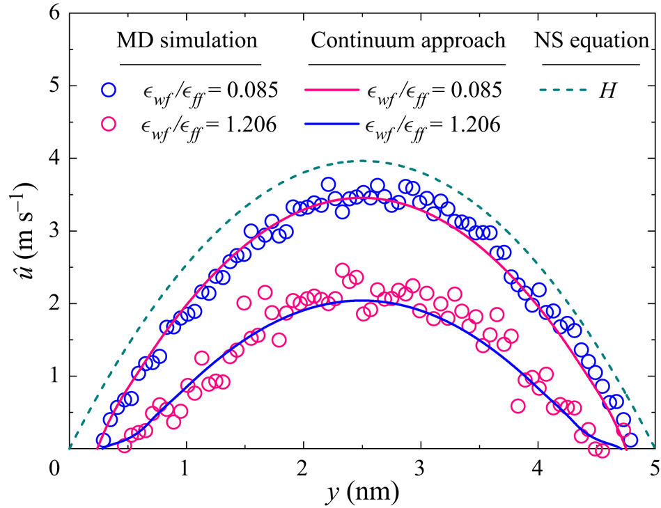
As discussed above, a slip boundary condition alone cannot accurately capture the flow dynamics in nanoscale systems. Here, with a slip velocity known a priori, the velocity distributions obtained from the present continuum model and the NS equation are compared for two different wettabilities. Again, the MD simulation results serve as the benchmark solution.

In the NS equation, the molecule size is not considered. So the depletion area, arising from the finite size of solid and fluid molecules, as well as the possibly strong repulsion between the solid and fluid molecules, is neglected in the NS equation. Therefore, the physical channel width (defined in figure 1 as $H$) should be kept equal for equivalent comparison, which means the effective channel width in the NS model is increased by the thickness of two depletion areas at the channel walls. From the computational perspective, the width of depletion area cannot be determined in the NS model, and the physical channel width should be chosen.

In figure 17, the velocity distributions across the channel are compared, where the velocity $\hat {u}$ is defined as

(4.9)

\begin{equation} \hat{u} = u-u_s, \end{equation}

where $u_s$ is the slip velocity. As shown in the figure, the velocity distribution across the channel depends on wettability. The fluid flows fast at the weak fluid–solid coupling, i.e. small $\epsilon _{wf}/\epsilon _{ff}$. In contrast, the effect of fluid–solid coupling is not considered in the NS equation and the simulated velocity is not affected by wettability, which deviates from the MD data, especially for large wettability, see figure 17. This indicates that a slip boundary condition alone cannot capture slip dynamics in strongly inhomogeneous nanoscale systems, where the fluid–fluid and fluid–solid molecular interactions need to be considered by the corresponding governing equations.

Figure 17.

A comparison of the present continuum model with the NS solutions. The MD results serve as the benchmark solution.

5. Conclusions

In this work, the molecular-kinetic boundary condition is developed to allow the generalised hydrodynamic model to probe the molecular-scale slip behaviours in nanoscale channels. In this continuum model, the molecular-scale slip characteristics are captured using the projected 12-6 LJ and 10-4-3 LJ potentials for the fluid–fluid and fluid–solid molecular interactions, which are consistent with those used in MD simulations. Therefore, the surface influence is also considered in the momentum equation as a mean-field force. A slip boundary condition alone is not sufficient to capture the molecular-scale fluid dynamics.

Slip length is found to decrease with density when the density is below the critical value, and increases with density at larger densities. This non-intuitive behaviour is a consequence of the force balance between surface friction and viscous force, reflecting competing fluid–solid and fluid molecular interactions. A universal scaling law for the slip length which captures the slip length minimum is proposed. The shear-rate dependent slip length is reproduced by the present continuum model, which shows the two distinctive slip regimes, i.e. the Navier slip regime at low shear rates, and the friction-reduction regime at high shear rates. The influence of temperature, density, channel width and fluid–surface coupling strength (i.e. wettability) on the slip length are also investigated. Interestingly, the slip length is found to increase with the channel width in a Couette flow, and to decrease in a Poiseuille flow before it becomes independent of the channel width when the channel width is beyond the critical value. The results show that the proposed slip boundary condition is applicable to different thermodynamic states and fluid–solid systems once the wettability factor $f_{wet}$ is calibrated.

The present continuum model provides an efficient and accurate method to simulate strongly inhomogeneous confined fluid flows at the nanoscale, which can describe both molecular-scale and macroscopic fluid dynamics. In comparison with MD, which is computationally costly, this continuum model can be used for large-scale practical simulations.

Acknowledgements

Valuable advice from Professor F. Wang of the University of Science and Technology of China about their MKT slip model is highly appreciated. B. Shan also thanks Dr Xiaocong Xu of the Hong Kong University of Science and Technology for helpful discussions.

Funding

This work is supported by the National Natural Science Foundation of China (grant no. 51836003 and no. 12002130). And funding support from the UK's Engineering and Physical Sciences Research Council under grant no. EP/R041938/1 is also acknowledged.

Declaration of interests

The authors report no conflict of interest.

Appendix A. Modelling of fluid–solid energy barrier

Fluid–solid molecular interaction is responsible for fluid adsorption and slip in the vicinity of the wall. Here, we attempt to develop a simplified model for the fluid–solid interaction, which can retain the essential physics. We employ a structureless plate to depict the role of fluid–solid interaction in the formation of adsorption layers, since adsorption is hardly affected by the lattice structure of the solid. As the fluid and solid molecules interact via 12-6 LJ potential (3.7), the total potential exerted by all the solid molecules on a fluid molecule can be calculated by an integration of the 12-6 potential over the whole solid surface, which is

(A1)

\begin{equation} \begin{aligned} E_{wf}(y) & = 4 n_w \epsilon_{wf}\int_{0}^{2{\rm \pi}}\,\mathrm{d}\omega \int_{0}^{+\infty}\left[\frac{\sigma_{wf}^{12}}{(r^2+y^2)^6} - \frac{\sigma_{wf}^6}{(r^2+y^3)^3}\right]r \,\mathrm{d} r\\ & = 2 n_w {\rm \pi}\epsilon_{wf} \sigma_{wf}^2\left[\frac{2}{5} \left(\frac{\sigma_{wf}}{y}\right)^{10} - \left(\frac{\sigma_{wf}}{y}\right)^4\right]. \end{aligned} \end{equation}

This is the so-called 10-4 LJ potential, acting upon a fluid molecule adjacent to the solid surface by all the wall molecules. We can see that solid–fluid molecular interaction depends on the perpendicular distance between the fluid molecule and the planar wall. This surface force is strongly repulsive when the distance is small, and becomes attractive when the fluid molecule moves away from the surface. This type of wall potential has been extensively used in the previous studies (Bitsanis et al. Reference Bitsanis, Magda, Tirrell and Davis1987; Guo et al. Reference Guo, Zhao and Shi2006a), and produced results in good agreement with the MD simulations. Under the influence of this potential, the fluid molecules would preferentially occupy the most stable positions, namely the locations with the lowest energy potential. Let $\partial E_{wf}/\partial y = 0$, the location of equilibrium sites with the lowest potential can be found at $y=\sigma _{wf}$.

Figure 18.

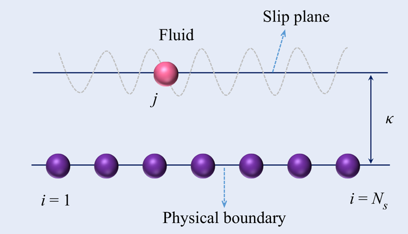
A schematic of numerical summation of the fluid–solid potential on the slip plane.

According to the MD studies (Thompson & Troian Reference Thompson and Troian1997; Lichter et al. Reference Lichter, Martini, Snurr and Wang2007; Martini et al. Reference Martini, Hsu, Patankar and Lichter2008a,Reference Martini, Roxin, Snurr, Wang and Lichterb), there should be some energy undulations in the flow direction due to the lattice structure of solid surfaces. The fluid density varies tangentially along the solid surface because fluid molecules preferentially occupy sites of lower energy over the solid surface. To encapsulate this mechanism, a small perturbation is implemented in the 10-4 LJ potential to generate energy corrugations along the flow direction. According to the previous studies (Martini et al. Reference Martini, Hsu, Patankar and Lichter2008a,Reference Martini, Roxin, Snurr, Wang and Lichterb; Hsu & Patankar Reference Hsu and Patankar2010), assuming that the energy corrugation satisfies a sine function with an amplitude of $e$, which is small compared with the total energy potential, the potential distribution over the solid surface can then be expressed as

(A2)

\begin{equation} E_{wf}(x, y) = E_{wf}(y)\left[1+e \sin\left(\frac{2 {\rm \pi}}{\delta} x\right)\right]. \end{equation}

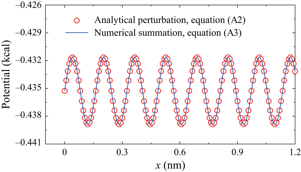
Here, we conduct numerical simulations to evaluate the accuracy of the perturbation described by a sinusoidal function in (A2). All the 12-6 fluid–solid interaction pairs between the solid and fluid molecules are summed numerically to compare with the analytical solution. Assuming there are $N_s$ solid molecules, the total potential exerted by all solid molecules on the position $j$ in the slip plane (see figure 18) can be calculated by summation as

(A3)

\begin{equation} \hat{E}_{wf}(j)= \sum_{i=1}^{N_s} \phi_{ij}, \end{equation}

where $\hat {E}_{wf}(j)$ is the potential that a fluid molecules ‘feels’ at an arbitrary position $j$ on the slip plane. The potential distribution along the slip plane can be obtained numerically, as shown in figure 19. The energy corrugation is well described by (A2), and the perturbation is small compared with the local average potential, i.e. $e \ll E_{wf}(\kappa )$, where $\kappa$ is the normal distance between the equilibrium sites and the solid surface, as shown in figure 2. At a constant height over the solid surface, the fluid molecules would experience a fluctuating potential as they pass over the discrete solid atoms (Steele Reference Steele1973). Therefore, this inhomogeneous potential in the surface of the first fluid layer dominates the slip dynamics at the boundary. In the bulk region, this energy corrugation can be ignored, since it decreases very rapidly (exponentially) with its distance to the wall.

Figure 19.

The energy corrugation over a solid surface: validation of the analytical perturbation given by (A2).

According to (A2), for an energy corrugation with the amplitude of $e$, the fluid–solid energy barrier depth $\Delta E_{wf}$ can be expressed as

(A4)

\begin{equation} \Delta E_{wf} = 2 e E_{wf}(\kappa). \end{equation}

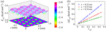
This demonstrates a linear relationship between the fluid–solid energy barrier depth $\Delta E_{wf}$ and the energy parameter $\epsilon _{wf}$ for a pair of solid–fluid molecules. In order to further prove this point, we take a two-dimensional graphene surface as an example. The total potential distribution in a surface at a distance $\kappa = 0.34$ nm from the solid is determined numerically by a superposition of each solid–fluid molecular interaction pair. This energy corrugation is clearly shown in figure 20($a$). In figure 20($b$), the linear relationship between $\Delta E_{wf}$ and $\epsilon _{wf}$ in surfaces at different distances from the solid ($\kappa = 0.32$ nm, $0.33$ nm and $0.34$ nm) is confirmed by the linear fitting between $\Delta E_{wf}$ and $\epsilon _{wf}$, i.e. the (3.9).

Figure 20.

($a$) The energy corrugation over a graphite solid at the equilibrium surface and ($b$) the relationship between the fluid–solid energy barrier depth $\Delta E_{wf}$ and the energy parameter $\epsilon _{wf}$ fitted by (3.9) with $a$ = 1.77, 1.07 and 0.66 for $\kappa$ = 0.32 nm, 0.33 nm and 0.34 nm, respectively.

For the multiple solid layers, the fluid–solid interactions can be described by the 10-4-3 LJ potential, also known as the Steele potential (Steele Reference Steele1973), which can be written as

(A5)

\begin{equation} E_{wf}(y)= 2 n_w {\rm \pi}\epsilon_{wf} \sigma_{wf}^2 L \left[\frac{2}{5} \left(\frac{\sigma_{wf}}{y}\right)^{10} - \left(\frac{\sigma_{wf}}{y}\right)^4 -\frac{\sigma_{wf}^4}{3L(y+0.61L)^3}\right], \end{equation}

where $L$ is the distance between adjacent solid plates. The relationship (3.9) still holds for the 10-4-3 LJ potential, which can be proved similarly as the 10-4 LJ potential.

Appendix B. Slip velocity and slip length in Couette flows

In a Couette flow, the shear stress $\tau = \eta (y)\gamma (y)$ should be a constant according to (2.5). Integrating (2.5) over the channel, the shear stress can be obtained as

(B1)

\begin{equation} \tau=\frac{2(u_w-u_s)}{\int_{0}^{H} \frac{1}{\eta(y)}\,\mathrm{d} y}. \end{equation}

Combining (3.12) and (B1), the slip velocity $u_s$ can be solved, after which the velocity across the channel can be obtained by

(B2)

\begin{equation} u|_{y=y_0}=u_w - u_s - \int_{y_0}^{H} \frac{\tau}{\eta(y)}\,\mathrm{d} y, \end{equation}

where $y_0$ is an arbitrary point in the channel. For a Couette flow, equation (2.7) for calculating the slip length reduces to

(B3)

\begin{equation} L_s = \frac{u_w}{\gamma}-\frac{H}{2}. \end{equation}

Appendix C. Slip velocity and slip length in Poiseuille flows

In a nanoscale confined Poiseuille flow, the shear stress is not explicitly specified. Integrating (2.6) and combining the symmetric condition $\gamma (y=H/2) = 0$, the shear stress distribution can be obtained as

(C1)

\begin{equation} \tau|_{y=y_0}=\left.\left(\eta \frac{{\rm d}u}{{\rm d} y}\right)\right|_{y=y_0} = G_x\int_{y_0}^{H/2}n(y)\,\mathrm{d} y, \end{equation}

from which we can see that the stress is related to the external force, the density distribution and the position. The stress at the bottom solid–fluid interface can be expressed as

(C2)

\begin{equation} \tau|_{y=0}=\left.\left(\eta \frac{{\rm d}u}{{\rm d} y}\right)\right|_{y=0} = G_x\int_{0}^{H/2}n(y)\,\mathrm{d} y=\frac{G_x n_{avg}H}{2}. \end{equation}

Substituting this stress into (3.12), the slip velocity can be determined. The velocity distribution can then be obtained according to (C1):

(C3)

\begin{equation} u|_{y=y_0} =\int_{0}^{y_0}\frac{\tau(y)}{\eta(y)}\,\mathrm{d} y+u_s. \end{equation}

For the Poiseuille flow, the slip length can be characterised by the apparent and intrinsic mass flow rate as

(C4)

\begin{equation} L_s=\frac{(Q_{app}/Q_{ins} -1) H}{6}, \end{equation}

where $Q_{app}$ and $Q_{ins}$ are the apparent and intrinsic mass flow rates, respectively. The intrinsic mass flow rate refers to flow satisfying Poiseuille law with a no-slip boundary condition, which is calculated by

(C5)

\begin{equation} Q_{ins}={-}\frac{\rho H^3w}{12\eta_{avg}}\boldsymbol{\nabla} p, \end{equation}

where $w$ is the width of nanochannel in the $z$ direction, and $\boldsymbol {\nabla } p$ is the pressure gradient related to external force by $-\boldsymbol {\nabla } p=G_x n$.

The apparent mass flow rate considers the effect of fluid density inhomogeneities and slip at the fluid–solid interface, which can be evaluated by

(C6)

\begin{equation} Q_{app} = w\int_{0}^{H} \rho(y)u(y)\,\mathrm{d} y. \end{equation}

Appendix D. The derivation of the friction coefficient

The derivation is divided into two regimes depending on the value of $({\tau S \delta })/{2k_BT}$. At small ${\tau S \delta }/{2k_BT}$, the hyperbolic function can be approximated by

(D1)

\begin{equation} \sinh\left(\frac{\tau S \delta}{2k_BT}\right)\approx\frac{\tau S \delta}{2k_BT}. \end{equation}

Consequently, the slip model (3.12) can be rewritten as

(D2)

\begin{equation} \tau = u_s \frac{h}{f_{wet}\delta^2S}\exp \left(\frac{a\epsilon_{wf}}{k_BT}\right). \end{equation}

According to the relationship $\tau =\zeta u_s$, the friction coefficient at small shear stress can be obtained as

(D3)

\begin{equation} \zeta=\frac{h}{f_{wet}\delta^2S}\exp \left(\frac{a\epsilon_{wf}}{k_BT}\right). \end{equation}

At large $({\tau S \delta })/{2k_BT}$, the hyperbolic function can be approximated by

(D4)

\begin{equation} \sinh\left(\frac{\tau S \delta}{2k_BT}\right)\approx \frac{1}{2}\exp \left(\frac{\tau S \delta}{2k_BT}\right), \end{equation}

and the slip model (3.12) can be rewritten as

(D5)

\begin{equation} \tau =\frac{2k_BT}{S\delta}\ln \left[u_s \frac{h}{k_BTf_{wet}\delta}\exp \left(\frac{a\epsilon_{wf}}{k_BT}\right)\right]. \end{equation}

Consequently, the friction coefficient at large stress can be evaluated by

(D6)

\begin{equation} \zeta=\frac{2k_BT}{S\delta u_s}\ln \left[u_s\frac{h}{k_BTf_{wet}\delta} \exp \left(\frac{a\epsilon_{wf}}{k_BT}\right) \right], \end{equation}

from which we can see that the friction coefficient depends on not only the system properties, but also the slip velocity at high shear stress. This corresponds to the friction reduction regime at high shear rate.

References

REFERENCES

Bailey, N.Y., Hibberd, S. & Power, H. 2017 Dynamics of a small gap gas lubricated bearing with Navier slip boundary conditions. J. Fluid Mech. 818, 68–99.CrossRef Google Scholar

Barisik, M. & Beskok, A. 2011 Equilibrium molecular dynamics studies on nanoscale-confined fluids. Microfluid. Nanofluid. 11 (3), 269–282.CrossRef Google Scholar

Barrat, J.L. & Bocquet, L. 1999 Large slip effect at a nonwetting fluid–solid interface. Phys. Rev. Lett. 82 (23), 4671–4674.CrossRef Google Scholar

Berthelot, D. 1898 Sur le mélange des gaz. Compt. Rendus 126, 1703–1706.Google Scholar

Bhadauria, R., Sanghi, T. & Aluru, N.R. 2015 Interfacial friction based quasi-continuum hydrodynamical model for nanofluidic transport of water. J. Chem. Phys. 143 (17), 174702.CrossRef Google Scholar PubMed

Bitrián, V. & Principe, J. 2018 Driving mechanisms and streamwise homogeneity in molecular dynamics simulations of nanochannel flows. Phys. Rev. Fluids 3 (1), 014202.CrossRef Google Scholar

Bitsanis, I., Magda, J.J., Tirrell, M. & Davis, H.T. 1987 Molecular dynamics of flow in micropores. J. Chem. Phys. 87 (3), 1733–1750.CrossRef Google Scholar

Bitsanis, I., Vanderlick, T.K., Tirrell, M. & Davis, H.T. 1988 A tractable molecular theory of flow in strongly inhomogeneous fluids. J. Chem. Phys. 89 (5), 3152–3162.CrossRef Google Scholar

Blake, T.D. & De Coninck, J. 2002 The influence of solid–liquid interactions on dynamic wetting. Adv. Colloid Interface Sci. 96 (1–3), 21–36.CrossRef Google Scholar PubMed

Cai, J.C., Zhang, Z.E., Wei, W., Guo, D.M., Li, S. & Zhao, P.Q. 2019 The critical factors for permeability-formation factor relation in reservoir rocks: pore-throat ratio, tortuosity and connectivity. Energy 188, 116051.CrossRef Google Scholar

Cao, B.Y., Chen, M. & Guo, Z.Y. 2006 Liquid flow in surface-nanostructured channels studied by molecular dynamics simulation. Phys. Rev. E 74 (6 Pt 2), 066311.CrossRef Google Scholar PubMed

Chapman, S & Cowling, T.G. 1970 The Mathematical Theory of Non-Uniform Gases. Cambridge University Press.Google Scholar

Cieplak, M., Koplik, J. & Banavar, J.R. 2001 Boundary conditions at a fluid–solid interface. Phys. Rev. Lett. 86 (5), 803–806.CrossRef Google Scholar

Dalton, B.A., Glavatskiy, K.S., Daivis, P.J. & Todd, B.D. 2015 Nonlocal response functions for predicting shear flow of strongly inhomogeneous fluids. II. Sinusoidally driven shear and multisinusoidal inhomogeneity. Phys. Rev. E 92 (1), 012108.CrossRef Google Scholar PubMed

Davis, T.H. 1987 Kinetic theory of flow in strongly inhomogeneous fluids. Chem. Engng Commun. 58 (1–6), 413–430.CrossRef Google Scholar

De Coninck, J. & Blake, T.D. 2008 Wetting and molecular dynamics simulations of simple liquids. Annu. Rev. Mater. Res. 38, 1–22.CrossRef Google Scholar

Evans, D.J. & Holian, B.L. 1985 The nose-hoover thermostat. J. Chem. Phys. 83 (8), 4069–4074.CrossRef Google Scholar

Falk, K., Sedlmeier, F., Joly, L., Netz, R.R. & Bocquet, L. 2010 Molecular origin of fast water transport in carbon nanotube membranes: superlubricity versus curvature dependent friction. Nano. Lett. 10 (10), 4067–4073.CrossRef Google Scholar PubMed

Germanou, L., Ho, M.T., Zhang, Y.H. & Wu, L. 2018 Intrinsic and apparent gas permeability of heterogeneous and anisotropic ultra-tight porous media. J. Nat. Gas Sci. Engng 60, 271–283.CrossRef Google Scholar

Glasstone, S., Laidler, K.J.S. & Eyring, H. 1941 The theory of rate processes: The kinetics of chemical reactions, viscosity, diffusion and electrochemical phenomena. Tech. Rep. McGraw-Hill Book Company.Google Scholar

Granick, S., Zhu, Y.X. & Lee, H. 2003 Slippery questions about complex fluids flowing past solids. Nat. Mater. 2 (4), 221–227.CrossRef Google Scholar PubMed

Guo, Z.L., Zhao, T.S. & Shi, Y. 2005 Simple kinetic model for fluid flows in the nanometer scale. Phys. Rev. E 71 (3), 035301.CrossRef Google Scholar PubMed

Guo, Z.L., Zhao, T.S. & Shi, Y. 2006 a Generalized hydrodynamic model for fluid flows: from nanoscale to macroscale. Phys. Fluids 18 (6), 067107.CrossRef Google Scholar

Guo, Z.L., Zhao, T.S., Xu, C. & Shi, Y. 2006 b Simulation of fluid flows in the nanometer: kinetic approach and molecular dynamic simulation. Intl J. Comput. Fluid Dyn. 20 (6), 361–367.CrossRef Google Scholar

Heiranian, M. & Aluru, N.R. 2020 Nanofluidic transport theory with enhancement factors approaching one. ACS Nano 14 (1), 272–281.CrossRef Google Scholar PubMed

Henot, M., Grzelka, M., Zhang, J., Mariot, S., Antoniuk, I., Drockenmuller, E., Leger, L. & Restagno, F. 2018 Temperature-controlled slip of polymer melts on ideal substrates. Phys. Rev. Lett. 121 (17), 177802.CrossRef Google Scholar PubMed

Ho, M.T., Li, J., Su, W., Wu, L., Borg, M., Li, Z. & Zhang, Y.H. 2020 Rarefied flow separation in microchannel with bends. J. Fluid Mech. 901, A26.CrossRef Google Scholar

Ho, T.A., Papavassiliou, D.V., Lee, L.L. & Striolo, A. 2011 Liquid water can slip on a hydrophilic surface. Proc. Natl Acad. Sci. USA 108 (39), 16170–16175.CrossRef Google Scholar PubMed

Ho, M.T., Zhu, L., Wu, L., Wang, P., Guo, Z., Li, Z. & Zhang, Y.H. 2019 b A multi-level parallel solver for rarefied gas flows in porous media. Comput. Phys. Commun. 234, 14–25.CrossRef Google Scholar

Ho, M.T., Zhu, L., Wu, L., Wang, P., Guo, Z., Ma, J. & Zhang, Y.H. 2019 a Pore-scale simulations of rarefied gas flows in ultra-tight porous media. Fuel 249, 341–351.CrossRef Google Scholar

Hocking, L.M. 1976 A moving fluid interface on a rough surface. J. Fluid Mech. 76 (4), 801–817.CrossRef Google Scholar

Holt, J.K., Park, H.G., Wang, Y.M., Stadermann, M., Artyukhin, A.B., Grigoropoulos, C.P., Noy, A. & Bakajin, O. 2006 Fast mass transport through sub-2-nanometer carbon nanotubes. Science 312 (5776), 1034–1037.CrossRef Google Scholar PubMed

Hsu, H.Y. & Patankar, N.A. 2010 A continuum approach to reproduce molecular-scale slip behaviour. J. Fluid Mech. 645, 59–80.CrossRef Google Scholar

Kannam, S.K., Todd, B.D., Hansen, J.S. & Daivis, P.J. 2013 How fast does water flow in carbon nanotubes? J. Chem. Phys. 138 (9), 094701.CrossRef Google Scholar PubMed

Kavokine, N., Netz, R.R. & Bocquet, L. 2021 Fluids at the nanoscale: from continuum to subcontinuum transport. Annu. Rev. Fluid Mech. 53, 377–410.CrossRef Google Scholar

Keerthi, A., et al. 2018 Ballistic molecular transport through two-dimensional channels. Nature 558 (7710), 420–424.CrossRef Google Scholar PubMed

Koplik, J., Banavar, J.R. & Willemsen, J.F. 1989 Molecular dynamics of fluid flow at solid surfaces. Phys. Fluids 1 (5), 781–794.CrossRef Google Scholar

Lauga, E. & Stone, H.A. 2003 Effective slip in pressure-driven stokes flow. J. Fluid Mech. 489, 55–77.CrossRef Google Scholar

Lichter, S., Martini, A., Snurr, R.Q. & Wang, Q. 2007 Liquid slip in nanoscale channels as a rate process. Phys. Rev. Lett. 98 (22), 226001.CrossRef Google Scholar PubMed

Lorentz, H.A. 1881 Ueber die anwendung des satzes vom virial in der kinetischen theorie der gase. Ann. Phys. 248 (1), 127–136.CrossRef Google Scholar

Ma, L., Gaisinskaya-Kipnis, A., Kampf, N. & Klein, J. 2015 Origins of hydration lubrication. Nat. Commun. 6, 6060.CrossRef Google Scholar PubMed

Ma, M.D., Shen, L.M., Sheridan, J., Liu, J.Z., Chen, C. & Zheng, Q.S. 2011 Friction of water slipping in carbon nanotubes. Phys. Rev. E 83 (3), 036316.CrossRef Google Scholar PubMed

Martini, A., Hsu, H.Y., Patankar, N.A. & Lichter, S. 2008 a Slip at high shear rates. Phys. Rev. Lett. 100 (20), 206001.CrossRef Google Scholar PubMed

Martini, A., Roxin, A., Snurr, R.Q., Wang, Q. & Lichter, S. 2008 b Molecular mechanisms of liquid slip. J. Fluid Mech. 600, 257–269.CrossRef Google Scholar

Mashayak, S.Y. & Aluru, N.R. 2012 Coarse-grained potential model for structural prediction of confined water. J. Chem. Theory Comput. 8 (5), 1828–1840.CrossRef Google Scholar PubMed

Morciano, M., Fasano, M., Nold, A., Braga, C., Yatsyshin, P., Sibley, D.N., Goddard, B.D., Chiavazzo, E., Asinari, P. & Kalliadasis, S. 2017 Nonequilibrium molecular dynamics simulations of nanoconfined fluids at solid-liquid interfaces. J. Chem. Phys. 146 (24), 244507.CrossRef Google Scholar PubMed

Nott, P.R. 2011 Boundary conditions at a rigid wall for rough granular gases. J. Fluid Mech. 678, 179–202.CrossRef Google Scholar

Patashinski, A.Z., Ratner, M.A., Orlik, R. & Mitus, A.C. 2019 Nanofluidic manifestations of structure in liquids: a toy model. J. Phys. Chem. C 123 (27), 16787–16795.CrossRef Google Scholar

Pozhar, L.A. & Gubbins, K.E. 1993 Transport theory of dense, strongly inhomogeneous fluids. J. Chem. Phys. 99 (11), 8970–8996.CrossRef Google Scholar

Priezjev, N.V. & Troian, S.M. 2006 Influence of periodic wall roughness on the slip behaviour at liquid/solid interfaces: molecular-scale simulations versus continuum predictions. J. Fluid Mech. 554 (1), 25–46.CrossRef Google Scholar

Richardson, S. 1973 On the no-slip boundary condition. J. Fluid Mech. 59 (4), 707–719.CrossRef Google Scholar

Ruckenstein, E. & Rajora, P. 1983 On the no-slip boundary condition of hydrodynamics. J. Colloid Interface Sci. 96 (2), 488–491.CrossRef Google Scholar

Secchi, E., Marbach, S., Nigues, A., Stein, D., Siria, A. & Bocquet, L. 2016 Massive radius-dependent flow slippage in carbon nanotubes. Nature 537 (7619), 210–213.CrossRef Google Scholar PubMed

Shan, B.C., Wang, P., Zhang, Y.H. & Guo, Z.L. 2020 Discrete unified gas kinetic scheme for all knudsen number flows. IV. Strongly inhomogeneous fluids. Phys. Rev. E 101, 043303.CrossRef Google Scholar PubMed

Sheng, Q., Gibelli, L., Li, J., K Borg, M.K. & Zhang, Y.H. 2020 Dense gas flow simulations in ultra-tight confinement. Phys. Fluids 32 (9), 544–550.CrossRef Google Scholar

Sholl, D.S. & Johnson, J.K. 2006 Materials science, making high-flux membranes with carbon nanotubes. Science 312 (5776), 1003–1004.CrossRef Google Scholar PubMed

Shu, J.J., Teo, J.B.M. & Chan, W.K. 2017 Fluid velocity slip and temperature jump at a solid surface. Appl. Mech. Rev. 69 (2), 020801.CrossRef Google Scholar

Śliwińska-Bartkowiak, M., Sterczyńska, A., Long, Y. & Gubbins, K.E. 2014 Influence of microroughness on the wetting properties of nano-porous silica matrices. Mol. Phys. 112 (17), 2365–2371.CrossRef Google Scholar

Sochi, T. 2011 Slip at fluid–solid interface. J. Polym. Rev. 51 (4), 309–340.CrossRef Google Scholar

Steele, W.A. 1973 The physical interaction of gases with crystalline solids: I. Gas-solid energies and properties of isolated adsorbed atoms. Surf. Sci. 36 (1), 317–352.CrossRef Google Scholar

Suk, M.E. & Aluru, N.R. 2017 Modeling water flow through carbon nanotube membranes with entrance/exit effects. Nanoscale Microscale Thermophys. Engng 21 (4), 247–262.CrossRef Google Scholar

Thompson, P.A. & Troian, S.M. 1997 A general boundary condition for liquid flow at solid surfaces. Nature 389 (6649), 360–362.CrossRef Google Scholar

Urbakh, M., Klafter, J., Gourdon, D. & Israelachvili, J. 2004 The nonlinear nature of friction. Nature 430 (6999), 525–528.CrossRef Google Scholar PubMed

Vanderlick, T.K., Scriven, L.E. & Davis, H.T. 1989 Molecular theories of confined fluids. J. Chem. Phys. 90 (4), 2422–2436.CrossRef Google Scholar

Voronov, R.S., Papavassiliou, D.V. & Lee, L.L. 2006 Boundary slip and wetting properties of interfaces: correlation of the contact angle with the slip length. J. Chem. Phys. 124 (20), 204701.CrossRef Google Scholar PubMed

Voronov, R.S., Papavassiliou, D.V. & Lee, L.L. 2008 Review of fluid slip over superhydrophobic surfaces and its dependence on the contact angle. Ind. Engng Chem. Res. 47 (8), 2455–2477.CrossRef Google Scholar

Wang, G.J. & Hadjiconstantinou, N.G. 2019 Universal molecular-kinetic scaling relation for slip of a simple fluid at a solid boundary. Phys. Rev. Fluids 4 (6), 064201.CrossRef Google Scholar

Wang, F.C. & Zhao, Y.P. 2011 Slip boundary conditions based on molecular kinetic theory: the critical shear stress and the energy dissipation at the liquid–solid interface. Soft Matt. 7 (18), 8628–8634.CrossRef Google Scholar

Wu, K., Chen, Z., Li, J., Li, X., Xu, J. & Dong, X. 2017 Wettability effect on nanoconfined water flow. Proc. Natl Acad. Sci. USA 114 (13), 3358–3363.CrossRef Google Scholar PubMed

Wu, L., Liu, H.H., Reese, J.M. & Zhang, Y.H. 2016 Non-equilibrium dynamics of dense gas under tight confinement. J. Fluid Mech. 794, 252–266.CrossRef Google Scholar

Wu, Y.Q., Tahmasebi, P., Lin, C.Y., Zahid, M.A., Dong, C.M., Golab, A.N. & Ren, L.H. 2019 A comprehensive study on geometric, topological and fractal characterizations of pore systems in low-permeability reservoirs based on SEM, MICP, NMR, and X-ray ct experiments. Mar. Petrol. Geol. 103, 12–28.CrossRef Google Scholar

Yang, F.Q. 2009 Slip boundary condition for viscous flow over solid surfaces. Chem. Engng Commun. 197 (4), 092003.CrossRef Google Scholar

Yao, L., Sanjayan, S., Song, J.L., Crick, C.R., Carmalt, C.J. & Parkin, I.P. 2015 Robust self-cleaning surfaces that function when exposed to either air or oil. Science 347 (6226), 1132–1135.Google Scholar

Yuan, Q.Z. & Zhao, Y.P. 2013 Multiscale dynamic wetting of a droplet on a lyophilic pillar-arrayed surface. J. Fluid Mech. 716, 171–188.CrossRef Google Scholar

Zampogna, G.A., Magnaudet, J. & Bottaro, A. 2018 Generalized slip condition over rough surfaces. J. Fluid Mech. 858, 407–436.CrossRef Google Scholar

Zhang, L.H., Shan, B.C., Zhao, Y.L. & Guo, Z.L. 2019 Review of micro seepage mechanisms in shale gas reservoirs. Intl J. Heat Mass Transfer 139, 144–179.CrossRef Google Scholar

Zhao, L. & Cheng, J.T. 2017 Analyzing the molecular kinetics of water spreading on hydrophobic surfaces via molecular dynamics simulation. Sci. Rep. 7 (1), 10880.CrossRef Google Scholar PubMed

Zhu, Y. & Granick, S. 2001 Rate-dependent slip of newtonian liquid at smooth surfaces. Phys. Rev. Lett. 87 (9), 096105.CrossRef Google Scholar PubMed

Figure 1.Schematic of a nanoscale Couette flow and illustration of molecular-scale slip at the surface: ($a$) division of flow regions according to the density distribution; ($b$) the true and extrapolated velocity of a Couette flow; ($c$) the relationship between the micro and apparent velocities.

Figure 2.The schematic of fluid molecules passing over a solid surface. ($a$) The total resistance from the fluid–solid interaction $\Delta E_{wf}$ and fluid–fluid molecular interaction $\Delta E_{ff}$. ($b$) The lattice structure of a solid wall and the related energy corrugations over the surface.

Figure 3.Schematic of the physical model in MD simulations.

Table 1.Input parameters of argon (Barisik & Beskok 2011) and graphene (Suk & Aluru 2017) for the continuum and MD simulations.

Figure 4.The dependency of wettability factor $f_{wet}$ on energy parameters ratio $\epsilon _{wf}/\epsilon _{ff}$. The fitting curve is (3.13) with $c_1=172.41$ and $c_2 = 1.28$.

Figure 5.The comparison of cross-sectional density and velocity distributions between our continuum and MD simulations at ($a$) $T$ = 253 K, ($b$) $T$ = 353 K and ($c$) $T$ = 453 K, respectively; and ($d$) comparison of the velocity profiles obtained by the continuum model at different temperatures.

Figure 6.The effect of temperature on the velocity profiles of the Poiseuille flows.

Figure 7.The effects of channel width $H$ on the slip length: ($a$) the Couette flow; and ($b$) the Poiseuille flow.

Figure 8.The effects of channel width $H$ on the normalised slip length and the resistance coefficient: ($a$) the Couette flow; and ($b$) the Poiseuille flow.

Figure 9.A comparison of the slip length predicted by our continuum and MD simulations at different wettability conditions: ($a$) the Couette flow; and ($b$) the Poiseuille flow.

Figure 10.A comparison of the slip length dependence on density between the continuum and MD simulations: ($a$) the Couette flow; and ($b$) the Poiseuille flow.

Figure 11.($a$) The variation of viscosity and friction coefficient with density, and ($b$) the competing effect of the fluid–solid and fluid–fluid molecular interactions on slip length.

Figure 12.A universal scaling law of slip length considering the effects of density, fluid–solid coupling strength, channel width and system temperature.

Figure 13.Dependency of the slip length on ($a$) density, ($b$) fluid–solid coupling strength and ($c$) comparison between our continuum model (symbols) and the general scaling law (4.6) of Thompson & Troian (1997) (dashed line).

Figure 14.The fluid slip length at low and high shear rates.

Figure 15.Using the continuum approach to simulate the slip flows of $\rho = 800\,{\rm kg}\,{\rm m}^{-3}$, $T= 353$ K, $H= 6$ nm over a wide range of fluid–solid coupling strengths.

Figure 16.Model comparison for slip velocity under different wettability, where the MD results serve as the benchmark solution.

Figure 17.A comparison of the present continuum model with the NS solutions. The MD results serve as the benchmark solution.

Figure 18.A schematic of numerical summation of the fluid–solid potential on the slip plane.

Figure 19.The energy corrugation over a solid surface: validation of the analytical perturbation given by (A2).

Figure 20.($a$) The energy corrugation over a graphite solid at the equilibrium surface and ($b$) the relationship between the fluid–solid energy barrier depth $\Delta E_{wf}$ and the energy parameter $\epsilon _{wf}$ fitted by (3.9) with $a$ = 1.77, 1.07 and 0.66 for $\kappa$ = 0.32 nm, 0.33 nm and 0.34 nm, respectively.

Article contents

Molecular kinetic modelling of nanoscale slip flow using a continuum approach

Abstract

JFM classification

Information

1. Introduction

2. Governing equation and molecular-scale slip

2.1. Generalised hydrodynamic model

2.2. Molecular scale slip

3. Slip mechanisms and molecular kinetic modelling

3.1. Slip mechanisms and related models

3.2. Effect of fluid molecular interactions on slip dynamics

3.3. Molecular kinetic modelling and analysis

4. Results and discussion

4.1. The wettability factor accounting for fluid molecular interactions

4.2. Effect of temperature on slip length

4.3. Effect of channel width on slip length

4.4. Effect of wettability on slip length

4.5. Effects of density on slip length

4.6. A scaling law for the slip length minimum

4.7. Slip length dependency on shear rate

4.8. Model analysis

4.9. A comparison with other slip models

4.10. Navier–Stokes equation with the current slip model

5. Conclusions

Acknowledgements

Funding

Declaration of interests

Appendix A. Modelling of fluid–solid energy barrier

Appendix B. Slip velocity and slip length in Couette flows

Appendix C. Slip velocity and slip length in Poiseuille flows

Appendix D. The derivation of the friction coefficient

References

REFERENCES

Save article to Kindle

Save article to Dropbox

Save article to Google Drive

Reply to: Submit a response

Your details

You have entered the maximum number of contributors

Conflicting interests