1 Introduction
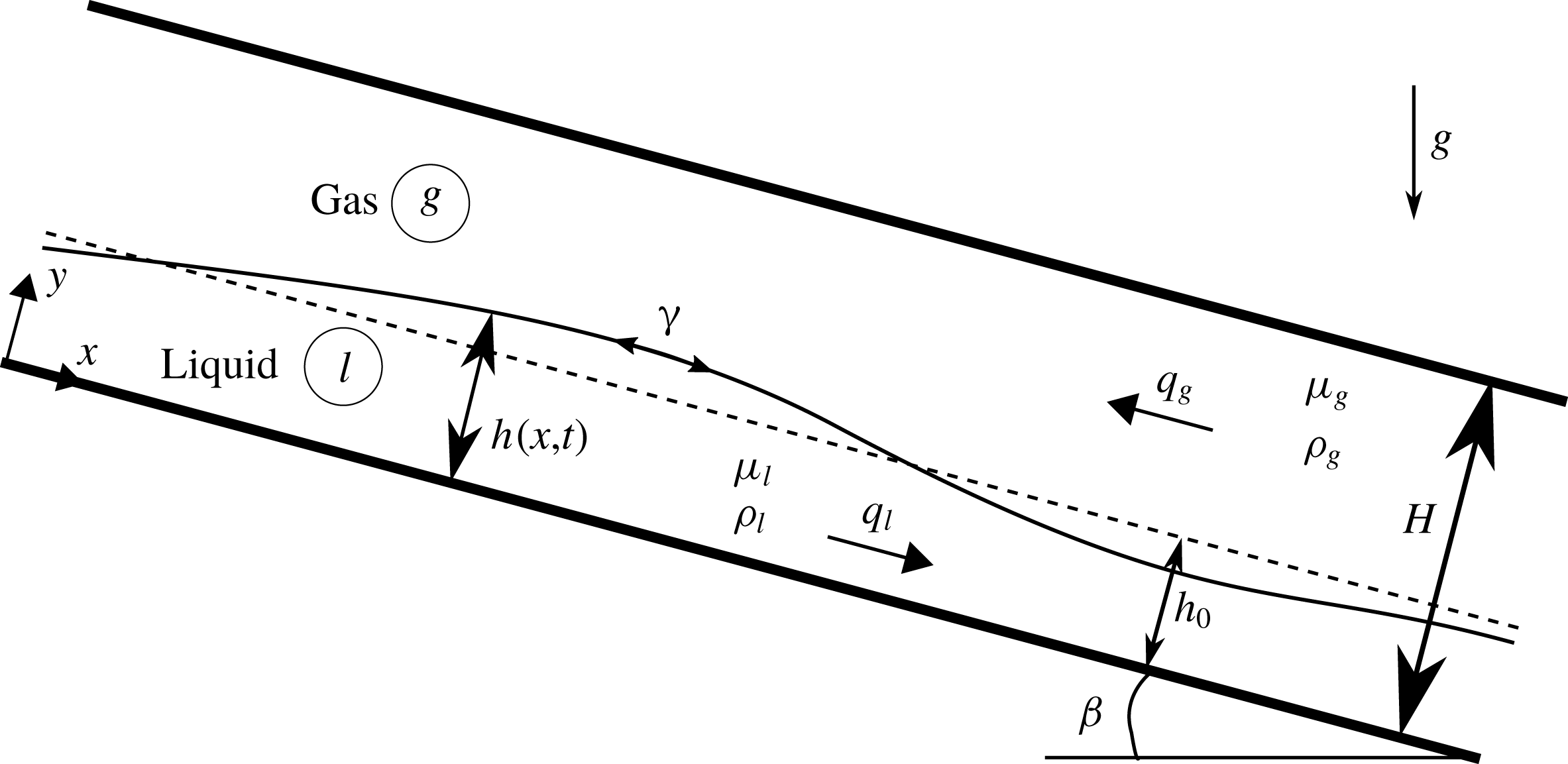
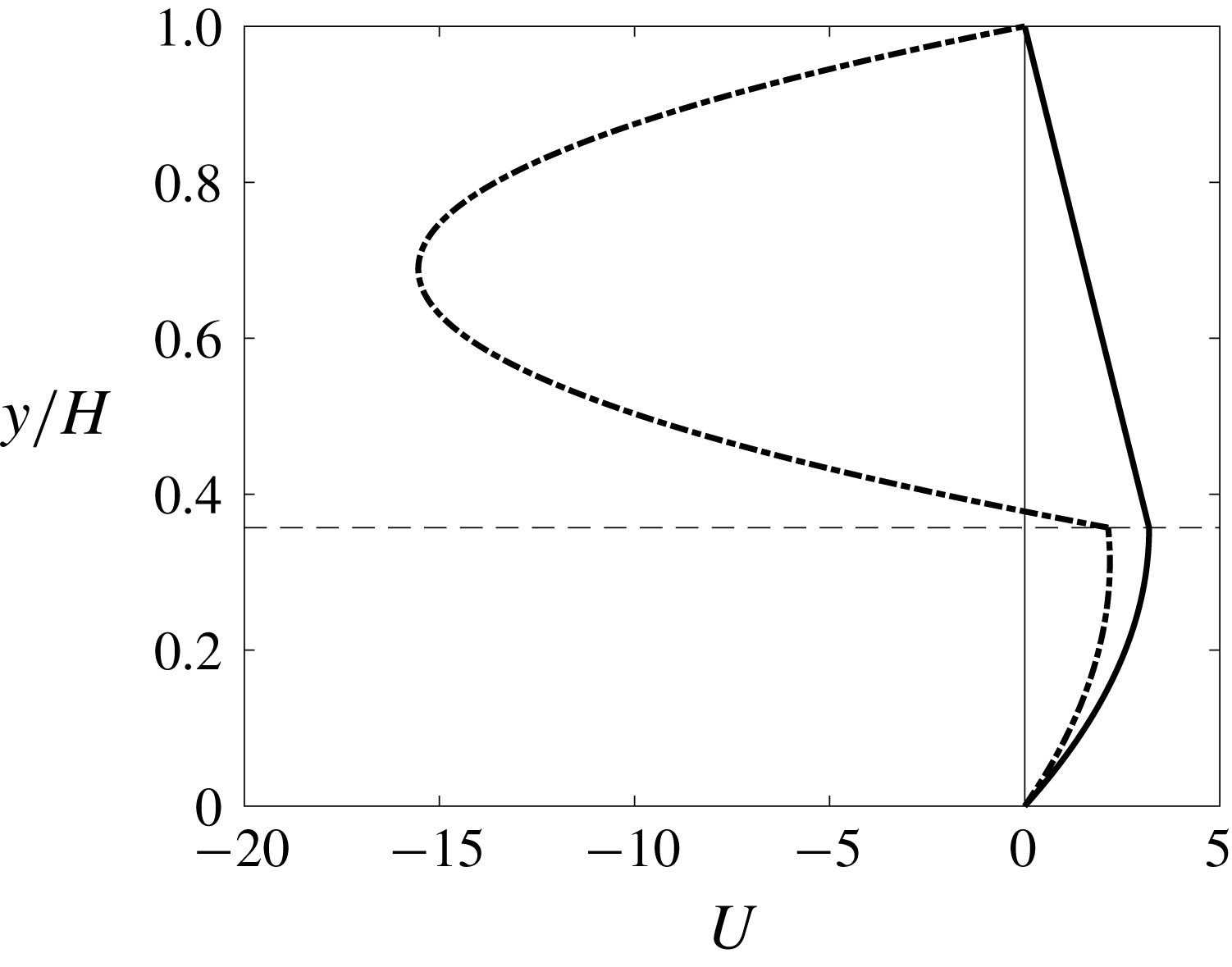
We consider a liquid film falling along the bottom wall of an inclined narrow channel, under the action of gravity and in interaction with a laminar gas flow (see figure 1). We distinguish two scenarios for the gas flow: either (i) the gas is subject to an aerostatic pressure gradient, i.e. a pressure difference which balances the weight of the gas column; or (ii) the gas flows counter-currently to the liquid film at an imposed flow rate. Examples of the velocity profiles corresponding to these two scenarios are depicted in figure 2. We revisit the linear stability of this flow by numerically solving the Orr–Sommerfeld temporal linear stability problem and by performing stability experiments. We are particularly interested in how the stability of the falling film is affected by the gas phase in the case of strong confinement. Among the susceptible instability modes of the film (Boomkamp & Miesen Reference Boomkamp and Miesen1996), we focus solely on the convective long-wave interfacial mode (Trifonov Reference Trifonov2017) known as Kapitza instability (Kapitza Reference Kapitza1948). For example, short-wave modes occurring in the liquid (Floryan, Davis & Kelly Reference Floryan, Davis and Kelly1987) and/or gas (Schmidt et al. Reference Schmidt, Ó Náraigh, Lucquiaud and Valluri2016) do not play a role in our study.
Sketch of the considered problem: a liquid film falling down an inclined wall whilst interacting with a strongly confined gas phase. The gas is either subject to an aerostatic pressure difference or flows counter-currently at an imposed flow rate. The flow rates
 $q_{l}$
and
 $q_{g}$
and the heights
 $h$
,
 $h_{0}$
and
 $H$
are dimensionless.

Base-state velocity profiles for an air–water flow:
 $\unicode[STIX]{x1D6FD}=3^{\circ }$
,
 $\unicode[STIX]{x1D702}=2.8$
(
 $\tilde{H}=1.5~\text{mm}$
). The horizontal dashed line represents the interface, the solid line is the aerostatic case (
 $M=1$
in (2.9)) with
 $Re_{l}=23.6$
, whereas the dash-dotted line is the counter-current case (
 $M=100$
in (2.9)) with
 $Re_{l}=17.1$
and
 $Re_{g}=-12.8$
.

We start by recalling some theoretical results for the case of a liquid film falling in a passive atmosphere. Benjamin (Reference Benjamin1957) and Yih (Reference Yih1963) solved the associated Orr–Sommerfeld temporal linear stability problem and proved that a vertical liquid film is always unstable to long-wave surface disturbances. Further, they determined the threshold of this long-wave instability in terms of the critical Reynolds number
 $Re_{cr}=(5/6)\cot \unicode[STIX]{x1D6FD}$
, which depends on the inclination angle
 $\unicode[STIX]{x1D6FD}$
. The instability mechanism is due to inertia, while the role of the longitudinal component of gravity is to advect and steepen the wave, whereas surface tension stabilizes the film. The way inertia destabilizes the film has been explained either via the shift between the vorticity and the displacement of the interface (Kelly et al.
Reference Kelly, Goussis, Lin and Hsu1989; Smith Reference Smith1990; Kalliadasis et al.
Reference Kalliadasis, Ruyer-Quil, Scheid and Velarde2012), following the argument introduced by Hinch (Reference Hinch1984) for two-layer Couette flows, or via the inertia-related lag of flow-rate perturbations with respect to film-thickness perturbations (Dietze Reference Dietze2016).
Investigations of the effect of an active outer phase on the stability of the film started with works dedicated to a slightly different configuration. Yih (Reference Yih1967) investigated the pressure-driven channel flow of two co-current fluid layers and showed that a viscosity contrast between layers of equal density and thickness causes a long-wave interfacial instability. This work was extended by Yiantsios & Higgins (Reference Yiantsios and Higgins1988), who accounted for a density contrast and a non-unity thickness ratio, and included gravity as well as surface tension. More recently, spatio-temporal linear stability analysis was applied to this problem (Valluri et al. Reference Valluri, Ó Náraigh, Ding and Spelt2010; Ó Náraigh, Spelt & Shaw Reference Ó Náraigh, Spelt and Shaw2013).
By additionally accounting for an inclination of the channel, Tilley, Davis & Bankoff (Reference Tilley, Davis and Bankoff1994) were able to investigate (among other scenarios) the stability of a falling water film in contact with air, which is the configuration we are interested in. In fact, their temporal Orr–Sommerfeld linear stability problem is exactly the same as the one we solve here (see § 2). The authors argued that confining the gas phase by an upper wall is likely to stabilize the falling film through an adverse shear stress at the liquid–gas interface. However, their calculations for the water–air system led them to conclude that this effect is negligible. Indeed, the minimum cutoff wavenumber upon varying the total flow rate changed only slightly with the channel height. In our current study, we have come to a different conclusion. We find that the cutoff wavenumber can be reduced up to the point of fully suppressing the Kapitza instability by diminishing the channel height at a fixed liquid flow rate. This holds both when the gas is subject to an aerostatic pressure difference and when it flows counter-currently.
A number of studies have investigated the effect of a turbulent counter-current gas flow on the stability of a falling liquid film. By applying a spatio-temporal analysis, Vellingiri, Tseluiko & Kalliadasis (Reference Vellingiri, Tseluiko and Kalliadasis2015) found a convective/absolute/upward-convective transition of the instability when increasing the interfacial shear stress exerted by the gas (conditions studied in our current paper are far removed from this transition). The authors also found that the cutoff wavenumber of the convective instability may either diminish, increase or display a non-monotonic behaviour with increasing gas shear stress. Trifonov (Reference Trifonov2017) made similar observations (also for turbulent gas flow) based on extensive temporal stability calculations, where the inclination angle, confinement and liquid Reynolds number were additionally varied. For the strong confinement levels on which we mainly focus in our current study, we have observed only a monotonic decrease of the cutoff wavenumber with increasing gas shear stress. However, we have checked that we recover the same qualitative behaviour as Vellingiri et al. (Reference Vellingiri, Tseluiko and Kalliadasis2015) and Trifonov (Reference Trifonov2017) when the confinement level is decreased, notwithstanding that the gas flow in our case is laminar and not turbulent.
We proceed by discussing several related experimental works that have focused on the linear stability of falling liquid films. Krantz & Goren (Reference Krantz and Goren1971) studied liquid films flowing down a strongly inclined plane at low Reynolds numbers. They imposed inlet disturbances of controlled amplitude and frequency, and measured wave celerities as well as spatial growth rates. Later, Pierson & Whitaker (Reference Pierson and Whitaker1977) and Alekseenko, Nakoryakov & Pokusaev (Reference Alekseenko, Nakoryakov and Pokusaev1985) studied liquid films flowing down the outside of a vertical cylinder. They measured the wavelength, wave celerity and spatial growth rate for the fastest-growing waves over a large range of Reynolds numbers, showing reasonable agreement with the theory developed in previous studies (Whitaker Reference Whitaker1964; Pierson & Whitaker Reference Pierson and Whitaker1977).
Liu, Paul & Gollub (Reference Liu, Paul and Gollub1993) studied liquid films falling down a weakly inclined plane at moderate Reynolds numbers. By imposing a small-amplitude perturbation of controlled frequency on the liquid flow rate, the authors were able to measure the critical Reynolds number in terms of the inclination angle, the cutoff wavenumber as a function of the Reynolds number, and the dispersion curves of the spatial growth rate and wave celerity. Their experimental data agreed with the neutral stability curve of Anshus & Goren (Reference Anshus and Goren1966).
Alekseenko et al. (Reference Alekseenko, Aktershev, Cherdantsev, Kharlamov and Markovich2009) investigated the additional effect of an active gas phase by measuring the spatial growth rate of small-amplitude surface waves excited on a liquid film falling down the inner surface of a vertical tube in interaction with a co- or counter-current turbulent gas flow. In particular, the authors found that increasing the counter-current gas flow reduces the cutoff wavenumber of the Kapitza instability, while the maximal growth rate is increased. Thus, shorter waves are stabilized while longer waves are amplified. Nonlinearly, this manifests itself in the attenuation of the precursory capillary ripples typically forming on wavy falling liquid films (Trifonov Reference Trifonov2010). This has also been detected experimentally by Kofman, Mergui & Ruyer-Quil (Reference Kofman, Mergui and Ruyer-Quil2017). We observe a different behaviour in our current study. For the strong confinement levels considered, we find that the linear growth rate is decreased at all unstable wavenumbers when the counter-current gas velocity is increased. However, in the case of a weaker confinement, we recover the same qualitative behaviour as Alekseenko et al. (Reference Alekseenko, Aktershev, Cherdantsev, Kharlamov and Markovich2009) for the laminar gas flow conditions studied here (see § 4.3).
Our paper is structured as follows. In § 2, we write the Orr–Sommerfeld temporal linear stability eigenvalue problem governing the stability of the falling film. The set-up and measurement methodology for the linear stability experiments are presented in § 3. In § 4 we present the results of our stability analysis, focusing on the stabilizing effect of confinement in terms of the liquid Reynolds number, the inclination angle, the Kapitza number and the velocity of a counter-current gas flow. The mechanism responsible for the stabilization induced by the confinement is presented in § 5. Finally, concluding remarks are presented in § 6.
2 Governing equations and linear stability problem
For the configuration depicted in figure 1, the governing equations in dimensionless form read as (subscripts
 $l$
and
 $g$
are phase indicators)
 $$\begin{eqnarray}\displaystyle & \displaystyle \unicode[STIX]{x1D735}\boldsymbol{\cdot }\boldsymbol{u}_{l}=0,\quad \unicode[STIX]{x1D735}\boldsymbol{\cdot }\boldsymbol{u}_{g}=0, & \displaystyle\end{eqnarray}$$
 $$\begin{eqnarray}\displaystyle & \displaystyle \text{D}_{t}\boldsymbol{u}_{l}=-\unicode[STIX]{x1D6F1}_{\unicode[STIX]{x1D70C}}\unicode[STIX]{x1D735}p_{l}+\boldsymbol{B}+\unicode[STIX]{x0394}\boldsymbol{u}_{l}, & \displaystyle\end{eqnarray}$$
 $$\begin{eqnarray}\displaystyle & \displaystyle \text{D}_{t}\boldsymbol{u}_{g}=-\unicode[STIX]{x1D735}p_{g}+\boldsymbol{B}+\unicode[STIX]{x1D6F1}_{\unicode[STIX]{x1D707}}\unicode[STIX]{x1D6F1}_{\unicode[STIX]{x1D70C}}^{-1}\unicode[STIX]{x0394}\boldsymbol{u}_{g}, & \displaystyle\end{eqnarray}$$
 $\unicode[STIX]{x1D6F1}_{\unicode[STIX]{x1D70C}}=\unicode[STIX]{x1D70C}_{g}/\unicode[STIX]{x1D70C}_{l}$
and
 $\unicode[STIX]{x1D6F1}_{\unicode[STIX]{x1D707}}=\unicode[STIX]{x1D707}_{g}/\unicode[STIX]{x1D707}_{l}$
designate the density and viscosity ratios. Here
 $\boldsymbol{u}$
is the velocity vector of components
 $(u,v)$
along
 $(x,y)$
,
 $p$
is the pressure,
 $\unicode[STIX]{x0394}$
is the Laplace operator,
 $\text{D}_{t}$
is the material derivative and
 $\boldsymbol{B}=(\sin \unicode[STIX]{x1D6FD},-\cos \unicode[STIX]{x1D6FD})$
is the inclination vector with the inclination angle
 $\unicode[STIX]{x1D6FD}$
. For non-dimensionalization, we have employed reference scales obtained from balancing viscous drag and gravity, i.e.
 ${\mathcal{L}}=\unicode[STIX]{x1D708}_{l}^{2/3}g^{-1/3}$
,
 ${\mathcal{U}}=(\unicode[STIX]{x1D708}_{l}g)^{1/3}$
and
 ${\mathcal{T}}={\mathcal{L}}/{\mathcal{U}}$
for length, velocity and time, and
 $\unicode[STIX]{x1D70C}_{g}{\mathcal{U}}^{2}$
for pressure. The reader is warned that the full gravitational acceleration
 $g$
rather than its streamwise projection
 $g_{x}=g\sin \unicode[STIX]{x1D6FD}$
is used here, in contrast to Ruyer-Quil & Manneville (Reference Ruyer-Quil and Manneville2000). This way, the scales are independent of the control parameters. As a result of our scaling, the Reynolds and Froude numbers do not appear explicitly in (2.1). We thus introduce the following definition for the Reynolds numbers in the liquid and gas:
 $$\begin{eqnarray}Re_{l}=\frac{\tilde{q}_{l}}{\unicode[STIX]{x1D708}_{l}},\quad Re_{g}=\frac{\tilde{q}_{g}}{\unicode[STIX]{x1D708}_{g}},\end{eqnarray}$$
where
 $\tilde{q}_{l}$
and
 $\tilde{q}_{g}$
are the dimensional liquid and gas flow rates per unit width (the tilde will denote dimensional quantities throughout the paper).
The boundary conditions at the walls read
 $$\begin{eqnarray}\boldsymbol{u}(0)=0,\quad \boldsymbol{u}(H)=0.\end{eqnarray}$$
The kinematic and dynamic coupling conditions at the interface
 $y=h$
are
 $$\begin{eqnarray}\displaystyle & \displaystyle u_{l}=u_{g}, & \displaystyle\end{eqnarray}$$
 $$\begin{eqnarray}\displaystyle & \displaystyle (\unicode[STIX]{x1D64E}_{l}\boldsymbol{\cdot }\boldsymbol{n})\boldsymbol{\cdot }\boldsymbol{t}=\unicode[STIX]{x1D6F1}_{\unicode[STIX]{x1D707}}(\unicode[STIX]{x1D64E}_{g}\boldsymbol{\cdot }\boldsymbol{n})\boldsymbol{\cdot }\boldsymbol{t}, & \displaystyle\end{eqnarray}$$
 $$\begin{eqnarray}\displaystyle & \displaystyle (\unicode[STIX]{x1D64E}_{l}\boldsymbol{\cdot }\boldsymbol{n})\boldsymbol{\cdot }\boldsymbol{n}+\unicode[STIX]{x1D705}We=\unicode[STIX]{x1D6F1}_{\unicode[STIX]{x1D70C}}(\unicode[STIX]{x1D64E}_{g}\boldsymbol{\cdot }\boldsymbol{n})\boldsymbol{\cdot }\boldsymbol{n}, & \displaystyle\end{eqnarray}$$
 $We=\unicode[STIX]{x1D6FE}(\unicode[STIX]{x1D70C}_{l}{\mathcal{L}}{\mathcal{U}}^{2})^{-1}$
is the Weber number with surface tension
 $\unicode[STIX]{x1D6FE}$
. Note that, due to the chosen scaling, our Weber number is identical to the Kapitza number
 $Ka=\unicode[STIX]{x1D6FE}(\unicode[STIX]{x1D70C}_{l}g^{1/3}\unicode[STIX]{x1D708}_{l}^{4/3})^{-1}$
which prevails in the literature on falling films. In (2.4b
) and (2.4c
),
 $\unicode[STIX]{x1D64E}=\unicode[STIX]{x1D64F}-p\unicode[STIX]{x1D644}$
is the stress tensor,
 $\unicode[STIX]{x1D64F}$
is the viscous stress tensor and
 $\unicode[STIX]{x1D644}$
is the identity matrix. The normal and tangential vectors to the interface are defined as
 $$\begin{eqnarray}\boldsymbol{n}=\frac{[-\unicode[STIX]{x2202}_{x}h,1]}{\sqrt{1+(\unicode[STIX]{x2202}_{x}h)^{2}}},\quad \boldsymbol{t}=\frac{[1,\unicode[STIX]{x2202}_{x}h]}{\sqrt{1+(\unicode[STIX]{x2202}_{x}h)^{2}}},\end{eqnarray}$$
whereas
 $\unicode[STIX]{x1D705}=\unicode[STIX]{x1D735}\boldsymbol{\cdot }\boldsymbol{n}=-\unicode[STIX]{x2202}_{xx}h[1+(\unicode[STIX]{x2202}_{x}h)^{2}]^{-3/2}$
is the curvature of the interface. The kinematic condition at the interface reads
 $$\begin{eqnarray}\unicode[STIX]{x2202}_{t}h+u_{l}\unicode[STIX]{x2202}_{x}h=v_{l}.\end{eqnarray}$$
In our analysis, we will vary the relative confinement of the film, which is defined as
 $$\begin{eqnarray}\unicode[STIX]{x1D702}=\frac{H}{h_{0}},\end{eqnarray}$$
where
 $h_{0}$
designates the film thickness of the primary flow and
 $H$
is the gap height. It constitutes one of the control parameters of the problem, together with the inclination angle
 $\unicode[STIX]{x1D6FD}$
and the flow rates
 $q_{l}$
and
 $q_{g}$
.
We perform a temporal stability analysis following the works of Yih (Reference Yih1967), Yiantsios & Higgins (Reference Yiantsios and Higgins1988) and Tilley et al. (Reference Tilley, Davis and Bankoff1994). We start by writing the base flow velocity profiles:
 $$\begin{eqnarray}\displaystyle U_{l} & = & \displaystyle K_{l}\Big(\frac{y^{2}}{2}-h_{0}y\Big)+\unicode[STIX]{x1D6F1}_{\unicode[STIX]{x1D70C}}T_{t}y,\end{eqnarray}$$
 $$\begin{eqnarray}\displaystyle U_{g} & = & \displaystyle K_{g}\frac{h_{0}^{2}}{2}\Big(\unicode[STIX]{x1D702}-\frac{y}{h_{0}}\Big)\Big(2-\unicode[STIX]{x1D702}-\frac{y}{h_{0}}\Big)-\frac{\unicode[STIX]{x1D6F1}_{\unicode[STIX]{x1D70C}}}{\unicode[STIX]{x1D6F1}_{\unicode[STIX]{x1D707}}}T_{t}h_{0}\Big(\unicode[STIX]{x1D702}-\frac{y}{h_{0}}\Big).\end{eqnarray}$$
 $K_{l}$
and
 $K_{g}$
are defined as
 $$\begin{eqnarray}\displaystyle & \displaystyle K_{l}=\unicode[STIX]{x1D6F1}_{\unicode[STIX]{x1D70C}}\unicode[STIX]{x2202}_{x}P-\sin \unicode[STIX]{x1D6FD}(1-\unicode[STIX]{x1D6F1}_{\unicode[STIX]{x1D70C}}M), & \displaystyle\end{eqnarray}$$
 $$\begin{eqnarray}\displaystyle & \displaystyle K_{g}=\unicode[STIX]{x1D6F1}_{\unicode[STIX]{x1D70C}}\unicode[STIX]{x1D6F1}_{\unicode[STIX]{x1D707}}^{-1}[\unicode[STIX]{x2202}_{x}P-\sin \unicode[STIX]{x1D6FD}(1-M)], & \displaystyle\end{eqnarray}$$
 $\unicode[STIX]{x2202}_{x}P$
is the driving pressure gradient and
 $M=\unicode[STIX]{x0394}p/\unicode[STIX]{x0394}p^{a}$
relates the driving pressure difference
 $\unicode[STIX]{x0394}p$
to the aerostatic pressure difference
 $\unicode[STIX]{x0394}p^{a}=\unicode[STIX]{x1D6EC}\sin \unicode[STIX]{x1D6FD}$
,
 $\unicode[STIX]{x1D6EC}$
designating the (dimensionless) wavelength. The coefficient
 $M$
allows one to distinguish between the two studied scenarios for the gas phase (see figure 2): (i) an aerostatic pressure difference, where
 $M=1$
; or (ii) a counter-current gas flow, where
 $M>1$
.
The interfacial tangential shear stress appearing in (2.8) is scaled with
 $\unicode[STIX]{x1D70C}_{g}{\mathcal{U}}^{2}$
and reads
 $$\begin{eqnarray}T_{t}=\frac{h_{0}}{2\unicode[STIX]{x1D6F1}_{\unicode[STIX]{x1D70C}}}[K_{l}-K_{g}(\unicode[STIX]{x1D702}-1)^{2}]\left[1+\frac{1}{\unicode[STIX]{x1D6F1}_{\unicode[STIX]{x1D707}}}(\unicode[STIX]{x1D702}-1)\right]^{-1},\end{eqnarray}$$
while the pressure profiles read
 $$\begin{eqnarray}\displaystyle & \displaystyle P_{l}=P|_{h_{0}}(x=0)+x\,\unicode[STIX]{x2202}_{x}P+\unicode[STIX]{x1D6F1}_{\unicode[STIX]{x1D70C}}^{-1}\cos \unicode[STIX]{x1D6FD}(h_{0}-y), & \displaystyle\end{eqnarray}$$
 $$\begin{eqnarray}\displaystyle & \displaystyle P_{g}=P|_{h_{0}}(x=0)+x\,\unicode[STIX]{x2202}_{x}P+\cos \unicode[STIX]{x1D6FD}(h_{0}-y), & \displaystyle\end{eqnarray}$$
 $P|_{h_{0}}(x=0)$
is an arbitrary reference pressure at
 $y=h_{0}$
and
 $x=0$
.
We linearly perturb the primary flow as follows:
 $$\begin{eqnarray}u=U+u^{\star },\quad v=v^{\star },\quad p=P+p^{\star },\end{eqnarray}$$
where upper-case letters refer to the base flow, while the star symbol denotes a small-amplitude perturbation. We introduce the streamfunction perturbations
 $\unicode[STIX]{x1D719}^{\star }$
in the liquid phase and
 $\unicode[STIX]{x1D713}^{\star }$
in the gas phase, satisfying
 $$\begin{eqnarray}\displaystyle u_{l}^{\star }=\unicode[STIX]{x2202}_{y}\unicode[STIX]{x1D719}^{\star },\quad v_{l}^{\star }=-\unicode[STIX]{x2202}_{x}\unicode[STIX]{x1D719}^{\star },\end{eqnarray}$$
 $$\begin{eqnarray}\displaystyle u_{g}^{\star }=\unicode[STIX]{x2202}_{y}\unicode[STIX]{x1D713}^{\star },\quad v_{g}^{\star }=-\unicode[STIX]{x2202}_{x}\unicode[STIX]{x1D713}^{\star },\end{eqnarray}$$
and seek solutions of the form
 $$\begin{eqnarray}\displaystyle & \displaystyle \{\unicode[STIX]{x1D719}^{\star },p_{l}^{\star }\}=\{\hat{\unicode[STIX]{x1D719}}(y),\hat{p}_{l}(y)\}\exp [\text{i}\unicode[STIX]{x1D6FC}(x-ct)], & \displaystyle\end{eqnarray}$$
 $$\begin{eqnarray}\displaystyle & \displaystyle \{\unicode[STIX]{x1D713}^{\star },p_{g}^{\star }\}=\{\hat{\unicode[STIX]{x1D713}}(y),\hat{p}_{g}(y)\}\exp [\text{i}\unicode[STIX]{x1D6FC}(x-ct)], & \displaystyle\end{eqnarray}$$
 $\unicode[STIX]{x1D6FC}\in \mathbb{R}$
is the wavenumber and
 $c=c_{r}+\text{i}c_{i}$
is the complex wave celerity, whereas the hat symbol denotes the amplitudes of the corresponding perturbations. Substituting (2.14) into (2.1) linearized around the base flow, and eliminating the pressure in (2.1b
) by substituting (2.1c
), we obtain the well-known Orr–Sommerfeld equations
 $$\begin{eqnarray}\displaystyle & \displaystyle \hat{\unicode[STIX]{x1D719}}^{\prime \prime \prime \prime }-2\unicode[STIX]{x1D6FC}^{2}\hat{\unicode[STIX]{x1D719}}^{\prime \prime }+\unicode[STIX]{x1D6FC}^{4}\hat{\unicode[STIX]{x1D719}}=\text{i}\unicode[STIX]{x1D6FC}[(U_{l}-c)(\hat{\unicode[STIX]{x1D719}}^{\prime \prime }-\unicode[STIX]{x1D6FC}^{2}\hat{\unicode[STIX]{x1D719}})-U_{l}^{\prime \prime }\hat{\unicode[STIX]{x1D719}}], & \displaystyle\end{eqnarray}$$
 $$\begin{eqnarray}\displaystyle & \displaystyle \hat{\unicode[STIX]{x1D713}}^{\prime \prime \prime \prime }-2\unicode[STIX]{x1D6FC}^{2}\hat{\unicode[STIX]{x1D713}}^{\prime \prime }+\unicode[STIX]{x1D6FC}^{4}\hat{\unicode[STIX]{x1D713}}=\text{i}\unicode[STIX]{x1D6FC}[(U_{g}-c)(\hat{\unicode[STIX]{x1D713}}^{\prime \prime }-\unicode[STIX]{x1D6FC}^{2}\hat{\unicode[STIX]{x1D713}})-U_{g}^{\prime \prime }\hat{\unicode[STIX]{x1D713}}], & \displaystyle\end{eqnarray}$$
 $$\begin{eqnarray}\displaystyle \hat{\unicode[STIX]{x1D719}}(0)=0,\quad \hat{\unicode[STIX]{x1D719}}^{\prime }(0)=0,\end{eqnarray}$$
 $$\begin{eqnarray}\displaystyle \hat{\unicode[STIX]{x1D713}}(H)=0,\quad \hat{\unicode[STIX]{x1D713}}^{\prime }(H)=0,\end{eqnarray}$$
where the prime symbol denotes differentiation with respect to
 $y$
. Linearization of the coupling conditions (2.4) must account for the perturbation of the variable fields as well as a perturbation of the position at which the condition is applied, i.e. at the interface. Consider the perturbed interfacial value
 $\{\,f\}|_{h}$
of the variable
 $f(x,y,t)$
with base state
 $F(y)$
. This can be decomposed into
 $$\begin{eqnarray}\{\,f\}|_{h}=\{F\}|_{h_{0}}+\{\,f^{\star }\}|_{h_{0}}+\{F^{\prime }\}|_{h_{0}}\,h^{\star },\end{eqnarray}$$
where
 $f^{\star }(x,y,t)=\,\hat{f}(y)\exp [\text{i}\unicode[STIX]{x1D6FC}(x-ct)]$
stems from the perturbation of the variable field and
 $\{F^{\prime }\}|_{h_{0}}\,h^{\star }$
is the contribution from changing the position of the film surface within this field.
Applying (2.18) to the coupling conditions (2.4) leads to
 $$\begin{eqnarray}\displaystyle & \displaystyle \hat{\unicode[STIX]{x1D719}}^{\prime }+U_{l}^{\prime }\hat{\unicode[STIX]{x1D719}}\text{}\underline{c}^{-1}=\hat{\unicode[STIX]{x1D713}}^{\prime }+U_{g}^{\prime }\hat{\unicode[STIX]{x1D719}}\text{}\underline{c}^{-1}, & \displaystyle\end{eqnarray}$$
 $$\begin{eqnarray}\displaystyle & \displaystyle \hat{\unicode[STIX]{x1D719}}^{\prime \prime }+U_{l}^{\prime \prime }\hat{\unicode[STIX]{x1D719}}\text{}\underline{c}^{-1}+\unicode[STIX]{x1D6FC}^{2}\hat{\unicode[STIX]{x1D719}}=\unicode[STIX]{x1D6F1}_{\unicode[STIX]{x1D707}}[\hat{\unicode[STIX]{x1D713}}^{\prime \prime }+U_{g}^{\prime \prime }\hat{\unicode[STIX]{x1D719}}\text{}\underline{c}^{-1}+\unicode[STIX]{x1D6FC}^{2}\hat{\unicode[STIX]{x1D713}}], & \displaystyle\end{eqnarray}$$
 $$\begin{eqnarray}\displaystyle & \displaystyle 2\unicode[STIX]{x1D6FC}^{2}\hat{\unicode[STIX]{x1D719}}^{\prime }-\text{i}\unicode[STIX]{x1D6FC}\unicode[STIX]{x1D6F1}_{\unicode[STIX]{x1D70C}}[\hat{p}_{l}+P_{l}^{\prime }\hat{\unicode[STIX]{x1D719}}\text{}\underline{c}^{-1}]+We\,\text{i}\unicode[STIX]{x1D6FC}^{3}\hat{\unicode[STIX]{x1D719}}\text{}\underline{c}^{-1}=2\unicode[STIX]{x1D6FC}^{2}\unicode[STIX]{x1D6F1}_{\unicode[STIX]{x1D707}}\hat{\unicode[STIX]{x1D713}}^{\prime }-\text{i}\unicode[STIX]{x1D6FC}\unicode[STIX]{x1D6F1}_{\unicode[STIX]{x1D70C}}[\hat{p}_{g}+P_{g}^{\prime }\hat{\unicode[STIX]{x1D719}}\text{}\underline{c}^{-1}],\qquad \quad & \displaystyle\end{eqnarray}$$
 $y=h_{0}$
and where we have introduced
 $\text{}\underline{c}=c-U|_{h_{0}}$
and used the relation
 $$\begin{eqnarray}h-h_{0}=h^{\star }=\hat{\unicode[STIX]{x1D719}}\text{}\underline{c}^{-1}\exp [\text{i}\unicode[STIX]{x1D6FC}(x-ct)],\end{eqnarray}$$
which follows directly from (2.6) together with (2.18). The pressure perturbation amplitudes
 $\hat{p}_{l}$
and
 $\hat{p}_{g}$
in (2.19c
), evaluated at
 $y=h_{0}$
, can be recovered directly from (2.1):
 $$\begin{eqnarray}\displaystyle & \displaystyle \hat{p}_{l}=\unicode[STIX]{x1D6F1}_{\unicode[STIX]{x1D70C}}^{-1}[\text{}\underline{c}\hat{\unicode[STIX]{x1D719}}^{\prime }+U_{l}^{\prime }\hat{\unicode[STIX]{x1D719}}]+(\text{i}\unicode[STIX]{x1D6FC}\unicode[STIX]{x1D6F1}_{\unicode[STIX]{x1D70C}})^{-1}(\hat{\unicode[STIX]{x1D719}}^{\prime \prime \prime }-\unicode[STIX]{x1D6FC}^{2}\hat{\unicode[STIX]{x1D719}}^{\prime }), & \displaystyle\end{eqnarray}$$
 $$\begin{eqnarray}\displaystyle & \displaystyle \hat{p}_{g}=[\text{}\underline{c}\hat{\unicode[STIX]{x1D713}}^{\prime }+U_{g}^{\prime }\hat{\unicode[STIX]{x1D713}}]+\unicode[STIX]{x1D6F1}_{\unicode[STIX]{x1D707}}(\text{i}\unicode[STIX]{x1D6FC}\unicode[STIX]{x1D6F1}_{\unicode[STIX]{x1D70C}})^{-1}(\hat{\unicode[STIX]{x1D713}}^{\prime \prime \prime }-\unicode[STIX]{x1D6FC}^{2}\hat{\unicode[STIX]{x1D713}}^{\prime }). & \displaystyle\end{eqnarray}$$
The Orr–Sommerfeld problem (2.15)–(2.21b
) is identical to the problem studied by Tilley et al. (Reference Tilley, Davis and Bankoff1994). We solve it by means of continuation using a code based on the continuation software AUTO-07p (Doedel Reference Doedel2008). This code was previously used in Dietze & Ruyer-Quil (Reference Dietze and Ruyer-Quil2013). The continuation is started from the asymptotic limit
 $\unicode[STIX]{x1D6FC}=0$
, for which
 $c_{r}$
and
 $c_{i}=0$
are known analytically, and continued by varying one of the control parameters while calculating
 $c_{r}$
and
 $c_{i}$
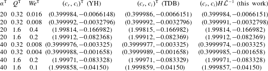
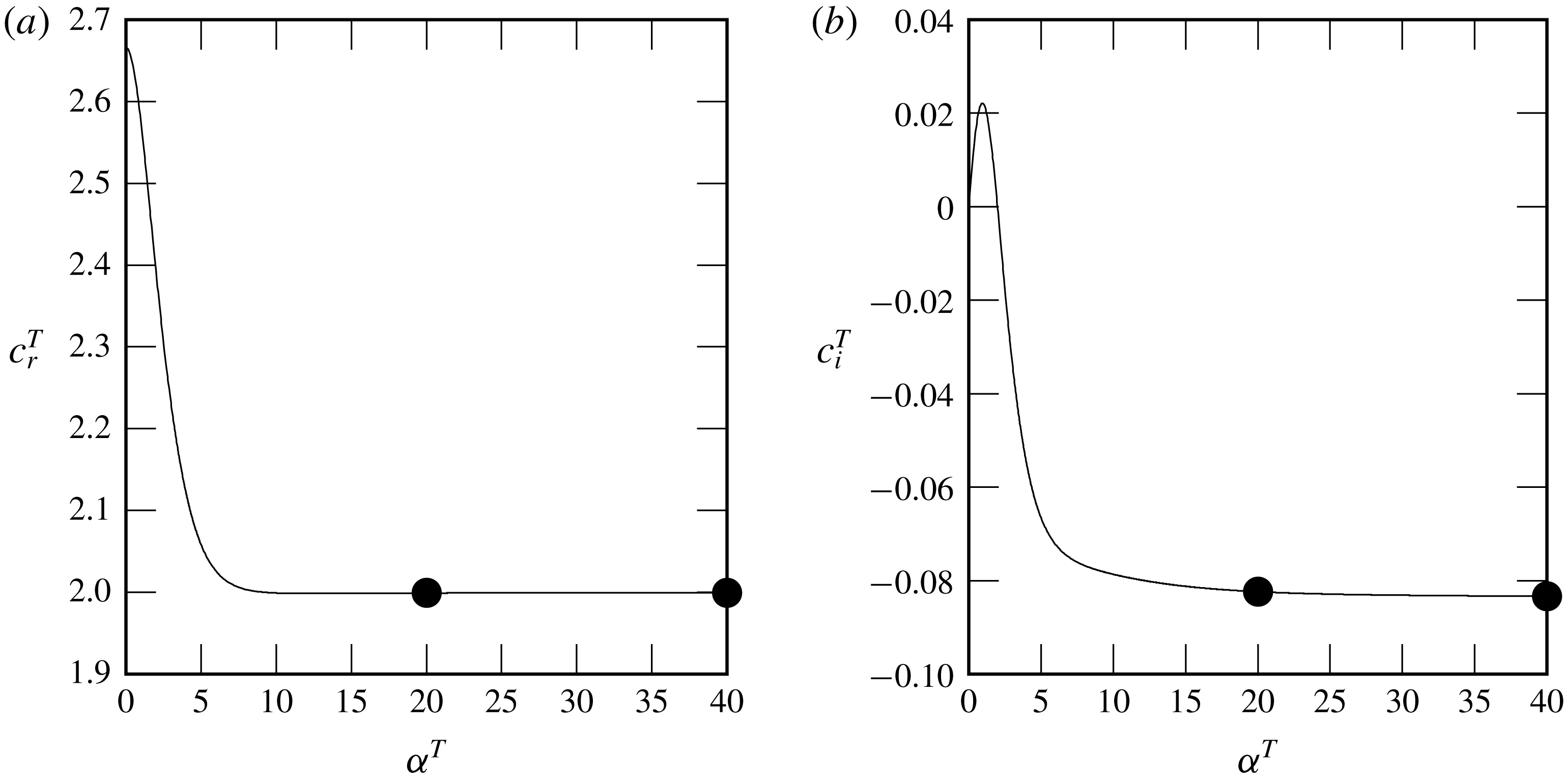
. We have validated our numerical procedure by comparing stability results with those of Brevdo et al. (Reference Brevdo, Laure, Dias and Bridges1999) for falling films in a passive atmosphere, those of Yiantsios & Higgins (Reference Yiantsios and Higgins1989) in the asymptotic limit of long waves, and those of Yiantsios & Higgins (Reference Yiantsios and Higgins1988) and Tilley et al. (Reference Tilley, Davis and Bankoff1994) for a pressure-driven horizontal liquid–gas flow. These validations are presented in appendix A.
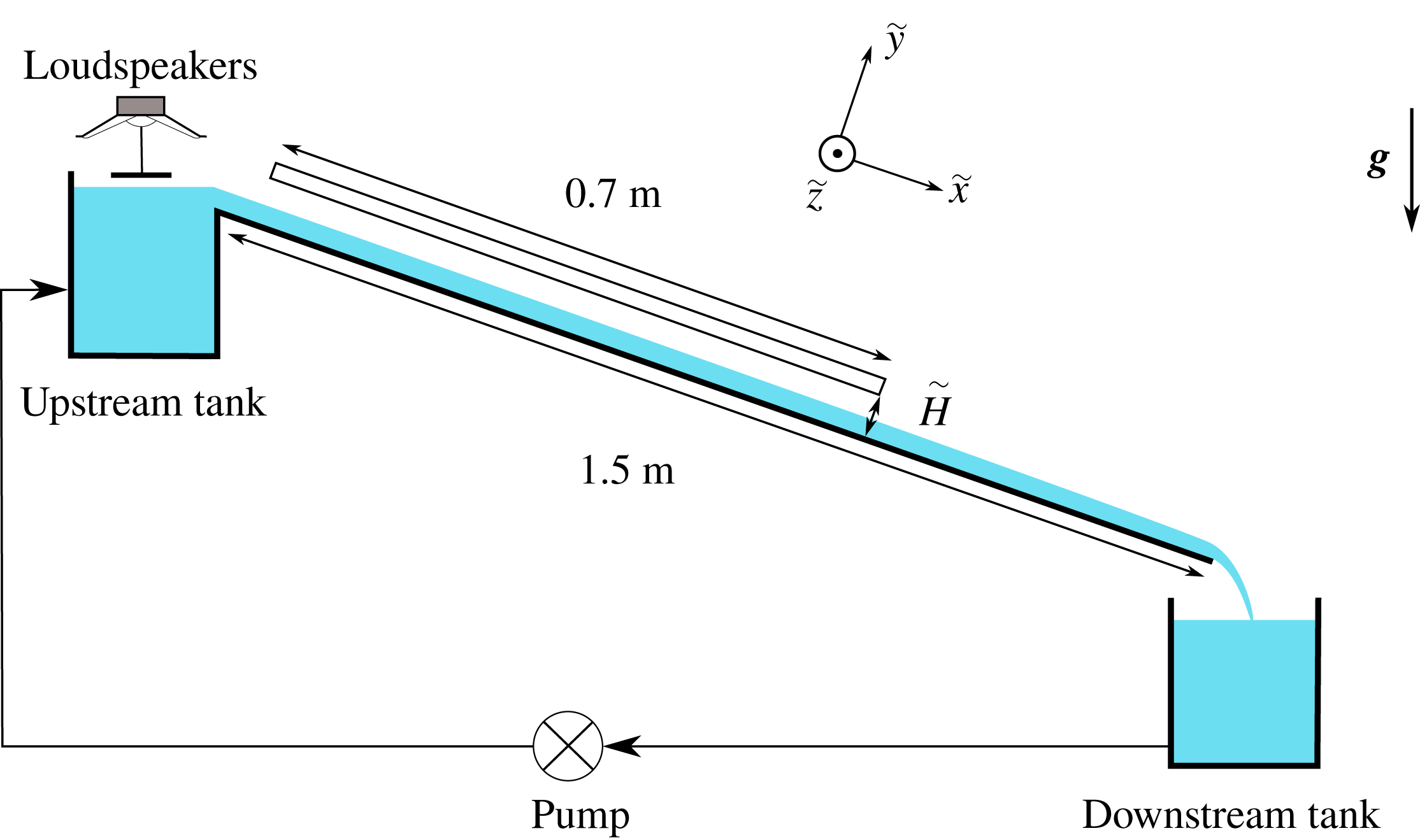
Sketch of the experimental set-up.

We point out that the considered gas flow rates are far from the convective-absolute transition studied by Vellingiri et al. (Reference Vellingiri, Tseluiko and Kalliadasis2015), Schmidt et al. (Reference Schmidt, Ó Náraigh, Lucquiaud and Valluri2016) and Lavalle et al. (Reference Lavalle, Vila, Lucquiaud and Valluri2017), thus no spatio-temporal analysis is required here. For additional security, we have validated our stability calculations with our own experiments, which are described in § 3. Owing to the convective nature of the instability, we measure a spatial growth rate in our experiments, whereas our stability calculations yield temporal growth rates (in a reference frame moving at the wave celerity). Both approaches yield the same stability threshold and most of our comparisons between experiments and linear stability analysis concern this stability threshold. However, in one instance (figure 9 b), we compare experimental and numerical growth-rate dispersion curves and for this we apply the so-called Gaster transformation (Gaster Reference Gaster1962) that relates temporal and spatial growth rates:
 $$\begin{eqnarray}\unicode[STIX]{x1D6FC}_{r}c_{i}=-\unicode[STIX]{x1D701}(c_{r}+\unicode[STIX]{x1D6FC}_{r}\unicode[STIX]{x2202}_{\unicode[STIX]{x1D6FC}_{r}}c_{r}),\end{eqnarray}$$
where
 $\unicode[STIX]{x1D701}$
is the spatial growth rate and
 $\unicode[STIX]{x1D6FC}_{r}c_{i}$
is the temporal one. This transformation is valid when the spatial and temporal growth rates are small. This is generally the case for falling liquid films, as shown by Brevdo et al. (Reference Brevdo, Laure, Dias and Bridges1999), who compared spatial growth rates obtained directly from a spatio-temporal analysis with values obtained by applying the Gaster transformation to temporal stability results, and showed that the error is less than
 $0.1\,\%$
. In the single instance where we have applied the Gaster transformation (figure 9
b), flow conditions are comparable to those in Brevdo et al. (Reference Brevdo, Laure, Dias and Bridges1999).
3 Experiments
Our experimental apparatus, sketched in figure 3, has been employed in previous studies (Kofman Reference Kofman2014; Kofman et al.
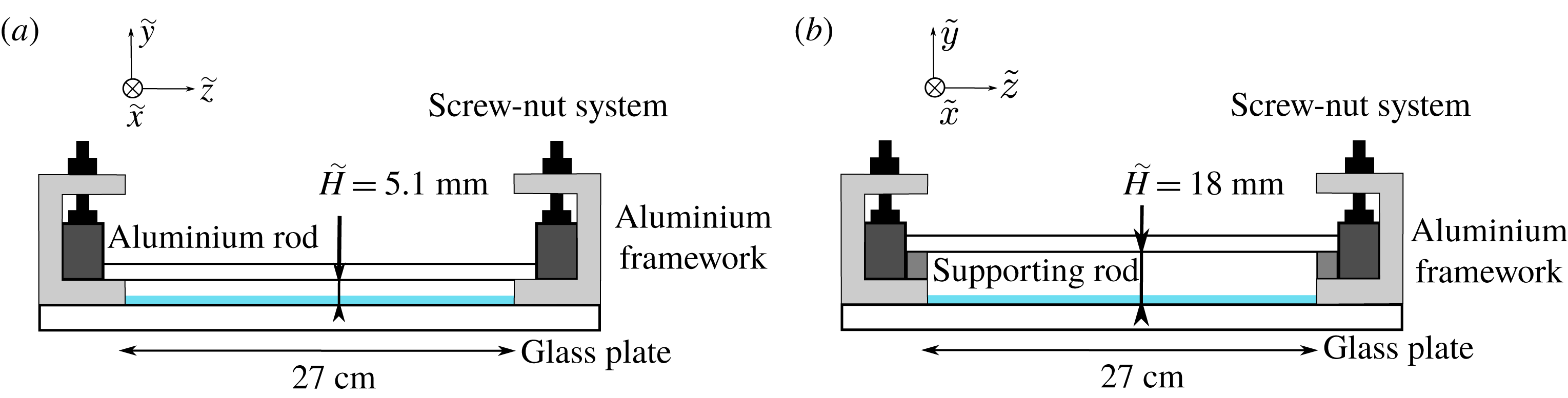
Reference Kofman, Mergui and Ruyer-Quil2017) and has been modified here to impose a much stronger confinement of the gas phase above the falling liquid film (figure 4). The liquid film flows down an inclined glass plate (
 $150~\text{cm}$
long,
 $27~\text{cm}$
wide,
 $5~\text{mm}$
thick) fixed in a framework mounted on rubber feet to reduce the influence of environmental vibrations. The inclination angle
 $\unicode[STIX]{x1D6FD}$
can be changed in the range
 $0^{\circ }$
–
 $20^{\circ }$
and is measured using an inclinometer with a precision of
 $0.05^{\circ }$
.
A gear pump conveys the liquid from a collection tank located at the end of the plate to an inlet tank, from which the liquid overflows onto the glass plate. The inlet tank is filled with several layers of glass beads in order to homogenize the entering flow. A temporal periodic forcing of the film is introduced at the inlet to trigger sinusoidal surface waves of prescribed frequency and amplitude. This is achieved by a vibrating aluminium plate, which is fixed to the membrane of two loudspeakers and generates harmonic vibrations above the liquid surface over the whole width of the film (Kofman et al. Reference Kofman, Mergui and Ruyer-Quil2017).
Sketch of the channel cross-section: (a) the confined and (b) the ‘unconfined’ configurations.

At a position
 $5~\text{cm}$
from the inlet, the falling film enters a region where the gas phase is confined by an upper
 $5~\text{mm}$
thick glass plate of length
 $70~\text{cm}$
and width
 $27~\text{cm}$
(see figure 3). In our study, the gap height
 $\tilde{H}$
of the channel formed between the two glass plates was set to two different values: (i)
 $\tilde{H}=5.1~\text{mm}\pm 0.1~\text{mm}$
, which we call the confined case; and (ii)
 $\tilde{H}=18~\text{mm}$
, which we loosely refer to as the ‘unconfined’ case. The shift from one case to the other is achieved by raising the top glass plate upon supporting rods (see figure 4). For the confined configuration, the uniformity of the gap height was verified in both the streamwise and the transverse directions.
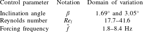
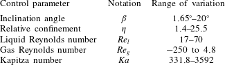
Water is used as working liquid. The temperature of the liquid is measured in the inlet and downstream tanks, and the surface tension is regularly monitored by measuring a water sample in a pendent drop tensiometer. The liquid flow rate is fixed large enough that the film is unstable but small enough that the film surface without inlet excitation is virtually flat in the measurement section (i.e. surface waves are undetectable). The experimental control parameters and the range of variation of the physical parameters are specified in tables 1 and 2.
Range of variation of the control parameters for the experiments.

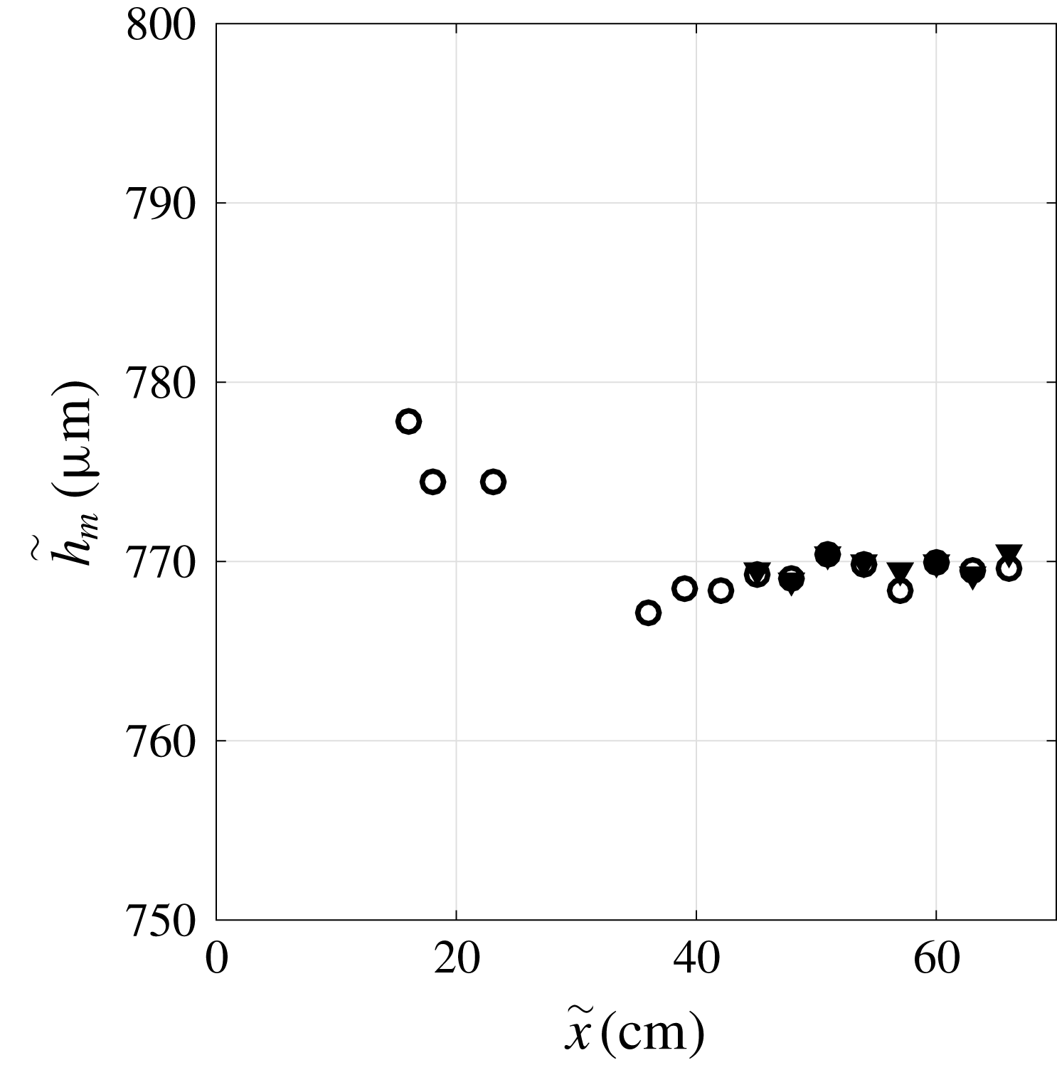
Streamwise evolution of the time-averaged film thickness
 $\tilde{h}_{m}$
along the central axis of the channel, with inlet excitation (
 $\tilde{f}=4.2~\text{Hz}$
, filled triangles) and without inlet excitation (empty circles). Parameters:
 $\unicode[STIX]{x1D6FD}=1.69^{\circ }$
,
 $Re_{l}=41.5$
, unconfined configuration
 $\tilde{H}=18~\text{mm}$
.

Physical properties of water at ambient temperature and their range of variation during the experiments.

To experimentally characterize the interfacial instability of the falling film, a one-point measurement of the film thickness time trace is performed using the confocal chromatic imaging (CCI) technique (Cohen-Sabban, Gaillard-Groleas & Crepin Reference Cohen-Sabban, Gaillard-Groleas, Crepin, Duparre and Singh2001). The sensor model used in our experiments (STIL CCS-PRIMA CL4) allows us to detect two interface locations simultaneously (the glass–water and the water–air interfaces) with a precision of 250 nm and an acquisition frequency up to 2 kHz. The CCI probe is mounted on a linear translation stage in order to enable measurements along the streamwise axis of the channel. The film thickness is measured at mid-width of the channel and at different longitudinal locations from the inlet. Measurements in the transverse direction were also carried out to check the uniformity of the film thickness, at sufficient distance from the lateral boundaries.
Figure 5 displays the streamwise evolution of the time-averaged film thickness
 $\tilde{h}_{m}$
along the central axis of the channel, in the unconfined configuration. Two wave regimes are represented: (i) a virtually flat film, observed without inlet excitation (empty circles), and (ii) periodically excited waves, observed with inlet forcing (filled triangles).
The actual flow rate of the falling liquid film is deduced from a film thickness measurement without inlet excitation, i.e. when the film surface is virtually flat. Indeed, for a fully developed waveless film, the film thickness
 $h_{0}$
and the Reynolds number
 $Re_{l}$
are linked through the base flow velocity profile (2.8) subject to an aerostatic pressure difference:
 $$\begin{eqnarray}Re_{l}=-K_{l}\frac{h_{0}^{3}}{3}+T_{t}\frac{h_{0}^{2}}{2},\end{eqnarray}$$
where
 $K_{l}$
is defined in (2.9a
) (using
 $M=1$
for the aerostatic scenario) and the interfacial tangential shear stress
 $T_{t}$
in (2.10). By measuring the film thickness without inlet excitation in the developed region of the film (where
 $\tilde{h}_{m}$
in figure 5 no longer changes), we obtain
 $Re_{l}$
from (3.1) with
 $h_{0}=h_{m}$
.
The same waveless signal also serves a second purpose. It is compared to the film thickness measured with inlet excitation to determine an upper limit for the excitation amplitude below which the excited surface waves can be considered linear, i.e. governed by the linearized Navier–Stokes equations (2.15). In that case, the film thickness perturbation is sinusoidal in time (2.20) and thus the time average of the perturbed film thickness
 $h_{0}+h^{\star }$
corresponds to the thickness of the waveless film
 $h_{0}$
. The excitation amplitude in the experiments was limited to values where this condition was satisfied in order to allow comparisons with the linear stability analysis.
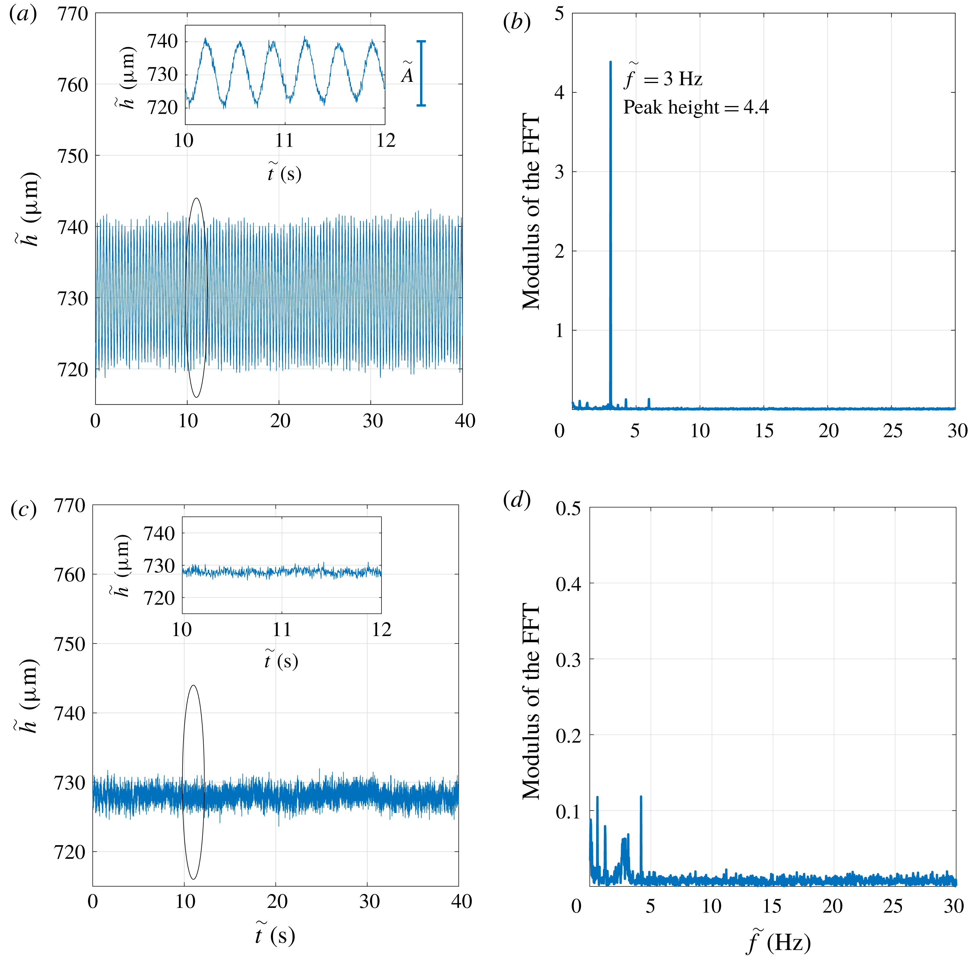
Consequently, the waves excited in our experiments were sinusoidal (see also inset in figure 6
a), and their amplitude
 $\tilde{A}$
, defined here as the peak-to-peak value of the time signal, can be obtained in a statistically robust manner by performing a discrete Fourier transform of the film thickness time trace measured with the CCI system.
The frequency resolution
 $\unicode[STIX]{x0394}f=f_{p}/N_{p}$
of the discrete Fourier analysis is limited by the acquisition frequency
 $f_{p}$
and the number of sampling points
 $N_{p}$
. In all our measurements, a minimum of five series of at least
 $80$
periods of the forcing mode were acquired. Thereby,
 $f_{p}$
and
 $N_{p}$
were chosen such that
 $\unicode[STIX]{x0394}f\leqslant 0.025~\text{Hz}$
. An example of the CCI signal and the corresponding modulus of the discrete Fourier transform are shown in figure 6(a,b). Here the forcing frequency is
 $3~\text{Hz}$
(
 $\unicode[STIX]{x1D6FD}=1.69^{\circ }$
,
 $Re_{l}=34.8$
). The predominant peak appearing in figure 6(b) indicates that the signal is mono-periodic with a frequency equal to the forcing frequency, as expected. The amplitude of this mode is directly obtained from the peak height, provided that the signal contains an integer number of periods of the relevant mode (Bergé, Pomeau & Vidal Reference Bergé, Pomeau and Vidal1988). Under this condition, the amplitude is four times the height of the peak (here
 $\tilde{A}=4\times 4.4=17.6~\unicode[STIX]{x03BC}\text{m}$
).
In figure 6(c,d) we have additionally represented a CCI signal and the corresponding spectrum obtained without inlet forcing for the same angle and Reynolds number as in figure 6(a,b). The spectrum exhibits peaks of very small amplitude (the scale has been divided by 10 compared to figure 6 b) that are the signature of the intrinsic noise of the set-up. The bump around 3 Hz and the low-frequency peaks are intrinsic to the set-up, as they are present in all our signals. The peak observed at 4.2 Hz is most probably due to the pump, the frequency of which increases with the Reynolds number, i.e. with the flow rate delivered by the pump. The noise level is low enough that the quality of the signal measured with inlet forcing is not deteriorated.
Examples of measurement signals with and without inlet forcing:
 $\unicode[STIX]{x1D6FD}=1.69^{\circ }$
,
 $Re_{l}=34.8$
, unconfined configuration
 $\tilde{H}=18~\text{mm}$
. (a) Time trace of the film thickness measured by the CCI system at a fixed longitudinal location
 $\tilde{x}=63~\text{cm}$
and enlarged inset. Forcing frequency:
 $\tilde{f}=3~\text{Hz}$
. (b) Corresponding modulus of the discrete Fourier transform. (c) Time evolution of the film thickness without inlet forcing. (d) Corresponding modulus of the discrete Fourier transform (the scale is divided by
 $10$
compared to panel (b)).

To investigate the linear stability of the film, we measure the spatial evolution of the wave amplitude along the channel. This allows us to obtain: (i) the spatial growth rate of the instability as a function of the forcing frequency for a given inclination angle and Reynolds number, i.e. the dispersion relation; and (ii) the cutoff frequency of the instability,
 $\tilde{f}_{c}$
, as a function of the Reynolds number for a given angle
 $\unicode[STIX]{x1D6FD}$
, i.e. the neutral stability curve
 $\tilde{f}_{c}(Re_{l})$
.
The spatial growth rate for a given frequency at a fixed (supercritical) Reynolds number is determined as follows. In the linear regime, the wave amplitude grows exponentially as a function of
 $\tilde{x}$
,
 $\tilde{A}(\tilde{x})\propto \exp (\tilde{\unicode[STIX]{x1D701}}\tilde{x})$
, where
 $\tilde{\unicode[STIX]{x1D701}}$
is the spatial growth rate and
 $\tilde{x}$
is the streamwise location of the measurement point. The spatial growth rate
 $\tilde{\unicode[STIX]{x1D701}}$
is obtained by performing a linear regression on the logarithm of
 $\tilde{A}(\tilde{x})$
. The precision of
 $\tilde{\unicode[STIX]{x1D701}}$
, i.e.
 $\unicode[STIX]{x0394}\tilde{\unicode[STIX]{x1D701}}$
, depends on the standard deviation of the residual of the regression,
 $\unicode[STIX]{x1D70E}_{res}$
, and on the length
 $\unicode[STIX]{x0394}\tilde{x}$
over which the measurements are conducted:
 $\unicode[STIX]{x0394}\tilde{\unicode[STIX]{x1D701}}=2\unicode[STIX]{x1D70E}_{res}\unicode[STIX]{x0394}\tilde{x}^{-1}$
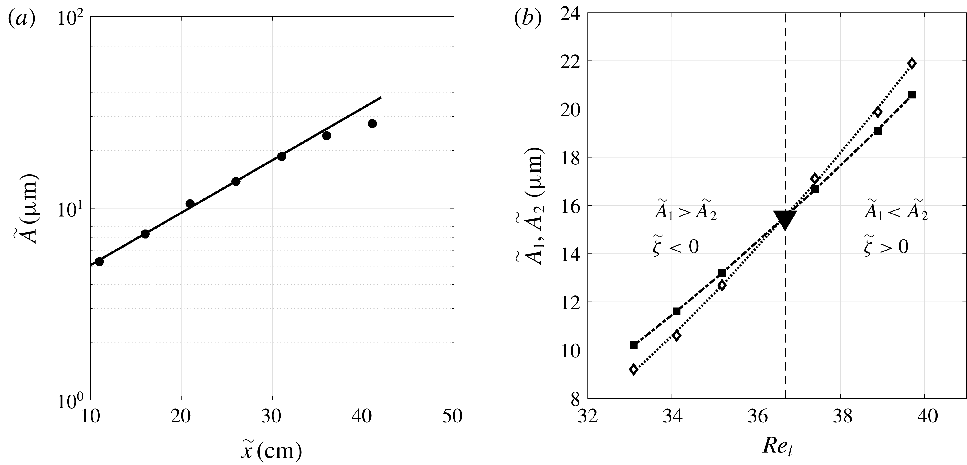
. These experiments require extremely precise amplitude measurements at several positions along the channel, especially when the growth rate is weak. Figure 7(a) shows an example of the streamwise spatial evolution of the wave amplitude. Here,
 $\tilde{\unicode[STIX]{x1D701}}$
is obtained by a fitting from
 $\tilde{x}=10$
to
 $30~\text{cm}$
. We observe that for
 $\tilde{x}>30~\text{cm}$
the spatial evolution of the wave amplitude is no longer exponential. The region of exponential growth varies depending on the experimental parameters (inclination angle, Reynolds number, forcing frequency). Accordingly, the amplitude of the inlet excitation is optimized for each experimental run so that the wave amplitude is large enough to be detected over the length of the channel while remaining in the linear regime.
Determining the growth rate and stability threshold from experiments. (a) The streamwise evolution of the wave amplitude along the channel (
 $\tilde{f}=2.6~\text{Hz}$
,
 $\unicode[STIX]{x1D6FD}=3.05^{\circ }$
,
 $Re_{l}=34.9$
, unconfined configuration
 $\tilde{H}=18~\text{mm}$
). Experimental points (circles) are fitted using an exponential curve (solid line) in the range
 $\tilde{x}=10{-}30~\text{cm}$
to obtain the spatial growth rate:
 $\tilde{\unicode[STIX]{x1D701}}=6.3~\text{m}^{-1}\pm 0.4~\text{m}^{-1}$
. (b) Determination of the critical Reynolds number from the change in wave amplitude at two streamwise locations
 $\tilde{x}_{1}$
and
 $\tilde{x}_{2}$
when varying
 $Re_{l}$
(
 $\tilde{f}=4.2~\text{Hz}$
,
 $\unicode[STIX]{x1D6FD}=1.69^{\circ }$
, unconfined configuration
 $\tilde{H}=18~\text{mm}$
). Filled squares, amplitude
 $\tilde{A}_{1}$
at
 $\tilde{x}_{1}=54~\text{cm}$
; empty diamonds, amplitude
 $\tilde{A}_{2}$
at
 $\tilde{x}_{2}=63~\text{cm}$
. The downward-pointing triangle marks the intersection, yielding the critical Reynolds number.

The neutral stability curve
 $\tilde{f}_{c}(Re_{l})$
is determined as follows. The wave amplitude is measured at two locations along the channel (amplitude
 $\tilde{A}_{1}$
at
 $\tilde{x}_{1}=54~\text{cm}$
and amplitude
 $\tilde{A}_{2}$
at
 $\tilde{x}_{2}=63~\text{cm}$
), within the exponential growth region. Fixing
 $\unicode[STIX]{x1D6FD}$
and the forcing frequency
 $\tilde{f}$
, we compare the two amplitudes for several Reynolds numbers to find the critical Reynolds number at which the spatial growth rate
 $\tilde{\unicode[STIX]{x1D701}}$
changes sign. This threshold is determined by fitting curves to the
 $\tilde{A}_{i}(Re_{l})$
data for the two locations and locating their intersection, as illustrated in figure 7(b). The two curves in figure 7(b) represents the wave amplitudes
 $\tilde{A}_{1}$
and
 $\tilde{A}_{2}$
measured at two different locations
 $\tilde{x}_{1}$
and
 $\tilde{x}_{2}>\tilde{x}_{1}$
as a function of
 $Re_{l}$
. At the value of
 $Re_{l}$
where the two curves intersect, i.e. where
 $\tilde{A}_{1}=\tilde{A}_{2}$
, the spatial growth rate is zero and thus
 $Re_{l}=Re_{cr}$
. To the left of the intersection, the downstream amplitude is smaller than the upstream one (
 $\tilde{A}_{1}>\tilde{A}_{2}$
) and thus the film is stable. To the right of the intersection, the downstream amplitude is larger than the upstream one (
 $\tilde{A}_{1}<\tilde{A}_{2}$
) and thus the film is unstable. This measurement of the critical Reynolds number is performed for several forcing frequencies, thus obtaining different points on the neutral stability curve
 $\tilde{f}_{c}(Re_{l})$
. Subsequently, in order to cross-validate these points, the Reynolds number is fixed at the critical value corresponding to a given forcing frequency, and frequencies slightly above and below this value are scanned to verify that the film indeed changes from stable to unstable.
4 Results
In this section, we present our experimental and numerical linear stability results for three existing fluid combinations: (i) water in contact with air, which we mainly focus on; (ii) aqueous solution of dimethylsulfoxide (DMSO) in contact with air; and (iii) aqueous solution of glycerin in contact with air. The fluid properties and the range of variation of the control parameters used for the numerical stability calculations are summarized in tables 3 and 4.
Physical properties of the fluid systems considered in the numerical stability calculations. The working liquids are: water, an aqueous solution of DMSO at 83.11 % by weight, and an aqueous solution of glycerin at 50 % by weight. The outer phase is air in all cases.

Range of variation of the control parameters for the numerical stability calculations.

4.1 Unconfined gas phase
We start by validating our temporal linear stability calculations with our experiments in the ‘unconfined’ configuration of figure 4(b) (
 $\tilde{H}=18~\text{mm}$
). We make this comparison for two types of curves: the neutral stability curve
 $\tilde{f}_{c}(Re_{l})$
and the dispersion curve of the spatial growth rate
 $\tilde{\unicode[STIX]{x1D701}}(\tilde{f})$
. In the latter case, we use the Gaster transformation (2.22) to transform the temporal growth rate from our numerical calculations into a spatial growth rate.
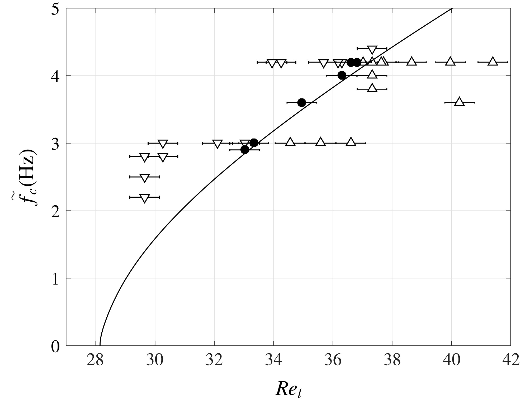
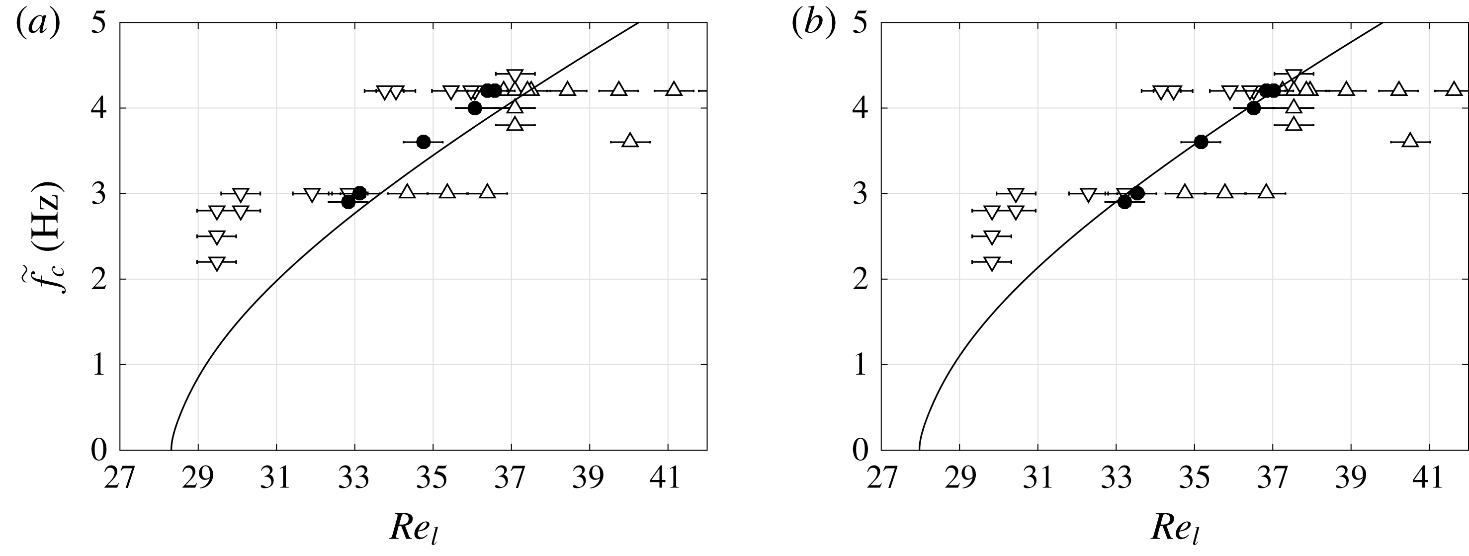
Comparison of numerical (line) and experimental (symbols) stability results at
 $\unicode[STIX]{x1D6FD}=1.69^{\circ }$
in the ‘unconfined’ configuration (figure 4
b): neutral stability curve. Symbols indicate the stability of the investigated point: downward-pointing triangles for stable, upward-pointing triangles for unstable, and circles for neutral conditions.

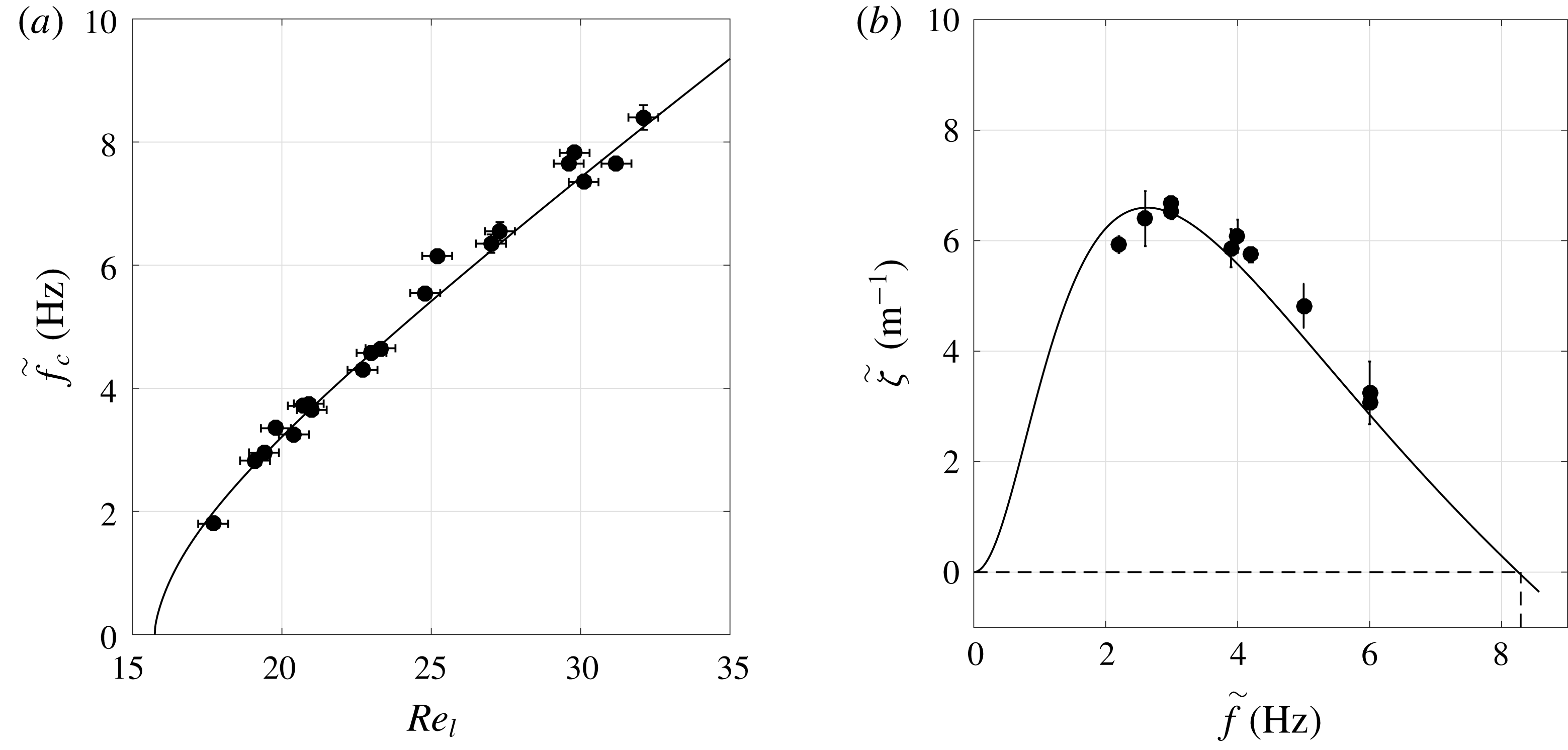
Comparison of numerical (solid line) and experimental (filled circles) stability results: unconfined configuration. (a) Neutral stability curve for
 $\unicode[STIX]{x1D6FD}=3^{\circ }$
; (b) dispersion curve of the spatial growth rate for
 $\unicode[STIX]{x1D6FD}=3.08^{\circ }$
and
 $Re_{l}=31$
. The precise value of
 $\unicode[STIX]{x1D6FD}$
is slightly different for the two panels, as experimental data were obtained from experimental runs on different days.

Figure 8 shows the neutral stability curve
 $\tilde{f}_{c}(Re_{l})$
for an inclination angle of
 $\unicode[STIX]{x1D6FD}=1.69^{\circ }$
. Therein, different types of symbols, which represent measurements, indicate the stability of the investigated point: downward-pointing triangles for stable, upward-pointing triangles for unstable, and circles for neutral conditions. The solid line corresponds to the stability calculation. We point out that the precision of the inclination angle measurement using the inclinometer was not sufficient to obtain such good agreement between the two datasets. Instead,
 $\unicode[STIX]{x1D6FD}$
, which is the same for all points on the neutral stability curve, was adjusted in the stability calculation until the numerical curve best matched the experimental one.
For the case of figure 8, where the inclinometer measurement yielded
 $\unicode[STIX]{x1D6FD}=1.70^{\circ }$
with a precision of
 $0.05^{\circ }$
, we computed numerical curves for inclination angles ranging from
 $1.67^{\circ }$
to
 $1.73^{\circ }$
with a
 $0.01^{\circ }$
increment. The numerical curve that fitted best with the experimental data yielded an inclination angle of
 $\unicode[STIX]{x1D6FD}=1.69^{\circ }$
. When varying
 $\unicode[STIX]{x1D6FD}$
, not only the numerical curve changes but also the experimental points, because the flow rate is obtained from equation (3.1), where
 $K_{l}$
depends on
 $\unicode[STIX]{x1D6FD}$
. To demonstrate the sensitivity of the comparison in figure 8 with respect to the inclination angle
 $\unicode[STIX]{x1D6FD}$
, we have included two additional figures in appendix B, showing the comparison for
 $\unicode[STIX]{x1D6FD}=1.68^{\circ }$
and
 $\unicode[STIX]{x1D6FD}=1.70^{\circ }$
.
Figure 9 compares numerical and experimental data for a larger inclination angle. Figure 9(a) represents the neutral stability curve for
 $\unicode[STIX]{x1D6FD}=3^{\circ }$
, and figure 9(b) the dispersion curve of the spatial growth rate for
 $\unicode[STIX]{x1D6FD}=3.08^{\circ }$
and
 $Re_{l}=31$
. As experimental data were not acquired on the same day, the precise value of
 $\unicode[STIX]{x1D6FD}$
is slightly different for the two panels. Agreement between the experimental and numerical dispersion curves confirms that the Gaster transformation is applicable here (see also Brevdo et al. (Reference Brevdo, Laure, Dias and Bridges1999)).
4.2 Confined gas phase: aerostatic pressure difference
We now study how the stability of the falling liquid film changes when the gas phase is significantly confined. To quantify the degree of confinement, we use the ratio
 $\unicode[STIX]{x1D702}$
(2.7) relating the gap height
 $H$
and the thickness of the primary film flow
 $h_{0}$
. To quantify the effect of
 $\unicode[STIX]{x1D702}$
on film stability, we will compare our stability results with the limiting case of a passive gas (
 $\unicode[STIX]{x1D6F1}_{\unicode[STIX]{x1D707}},\unicode[STIX]{x1D6F1}_{\unicode[STIX]{x1D70C}}\rightarrow 0$
), where the confinement plays no role. This limit will be denoted with the superscript
 $\infty$
.
We first study the situation where the gas is subject to an aerostatic pressure gradient. In that case, the gas moves only as a reaction to the film’s motion. We start by validating our temporal stability calculations with our own experiments in the confined configuration
 $\tilde{H}=5.1~\text{mm}$
(figure 4
a) and the ‘unconfined’ configuration
 $\tilde{H}=18~\text{mm}$
(figure 4
b) at an inclination angle
 $\unicode[STIX]{x1D6FD}=1.69^{\circ }$
, using water as working liquid.
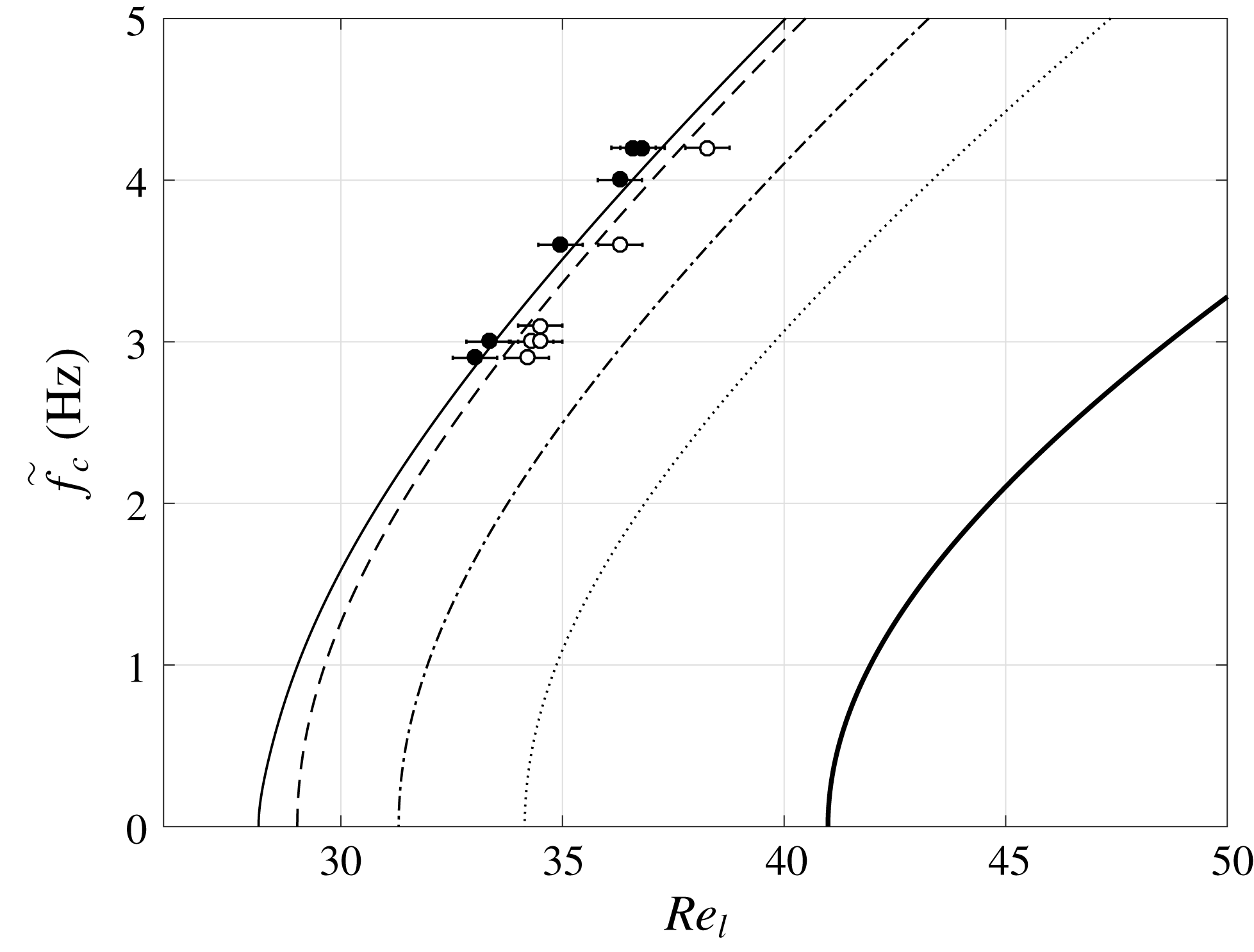
The two leftmost curves in figure 10 represent the calculated neutral stability curves
 $\tilde{f}_{c}(Re_{l})$
for these two configurations, while symbols represent the corresponding experimental data. Both datasets evidence a clear stabilization of the falling film due to increased confinement of the gas phase (dashed curve, open circles), and their agreement is gratifying.
The dimensional gap height
 $\tilde{H}$
along the curves in figure 10 is constant, meaning that the relative confinement
 $\unicode[STIX]{x1D702}$
changes, as
 $\tilde{h}_{0}$
changes with
 $Re_{l}$
. Nonetheless, a representative value for
 $\unicode[STIX]{x1D702}$
can be given for each curve by evaluating it at the critical Reynolds number
 $Re_{cr}$
(where the curve intersects the
 $x$
-axis), i.e.
 $\unicode[STIX]{x1D702}_{cr}=\unicode[STIX]{x1D702}(\unicode[STIX]{x1D6FC}_{c}=0)$
,
 $\unicode[STIX]{x1D6FC}_{c}$
being the cutoff wavenumber. The quantity
 $\unicode[STIX]{x1D702}_{cr}$
is quite large for the two leftmost curves in figure 10 (
 $\unicode[STIX]{x1D702}_{cr}>7$
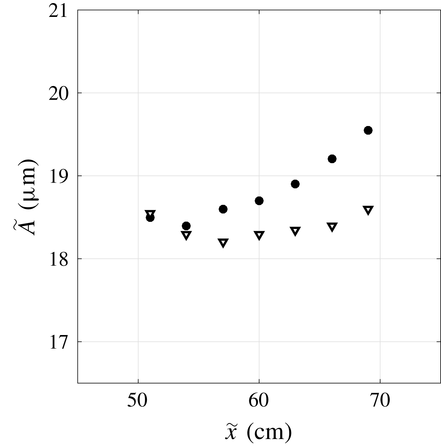
), and this explains why the observed confinement-induced stabilization is rather weak (experimental wave amplitudes are reported in figure 24 of appendix C). However, when decreasing
 $\unicode[STIX]{x1D702}_{cr}$
, the confinement-induced stabilization becomes much stronger, as evidenced by the three additional curves in figure 10 obtained from our stability calculations. For example, at
 $\unicode[STIX]{x1D702}_{cr}=2.23$
(thick solid line), the critical Reynolds number
 $Re_{cr}$
, below which the film is always stable, is increased by over
 $50\,\%$
compared to the ‘unconfined’ configuration (thin solid line).
Neutral stability curves of a water film (
 $Ka=3592$
) inclined at
 $\unicode[STIX]{x1D6FD}=1.69^{\circ }$
in contact with aerostatic air at different confinement levels
 $\unicode[STIX]{x1D702}_{cr}=\unicode[STIX]{x1D702}(\unicode[STIX]{x1D6FC}_{c}=0)$
. Filled symbols, ‘unconfined’ experiment with
 $\unicode[STIX]{x1D702}_{cr}=25.5$
(figure 4
b,
 $\tilde{H}=18~\text{mm}$
); open symbols, confined experiment with
 $\unicode[STIX]{x1D702}_{cr}=7.54$
(figure 4
a,
 $\tilde{H}=5.1~\text{mm}$
). Stability calculations are represented with lines. Thin solid line, ‘unconfined’ (
 $\unicode[STIX]{x1D702}_{cr}=25.5$
,
 $\tilde{H}=18~\text{mm}$
); dashed line, confined at
 $\tilde{H}=5.1~\text{mm}$
(
 $\unicode[STIX]{x1D702}_{cr}=7.54$
); dash-dotted line,
 $\tilde{H}=2.5~\text{mm}$
(
 $\unicode[STIX]{x1D702}_{cr}=3.60$
); dotted line,
 $\tilde{H}=2~\text{mm}$
(
 $\unicode[STIX]{x1D702}_{cr}=2.80$
); thick solid line,
 $\tilde{H}=1.7~\text{mm}$
(
 $\unicode[STIX]{x1D702}_{cr}=2.23$
).

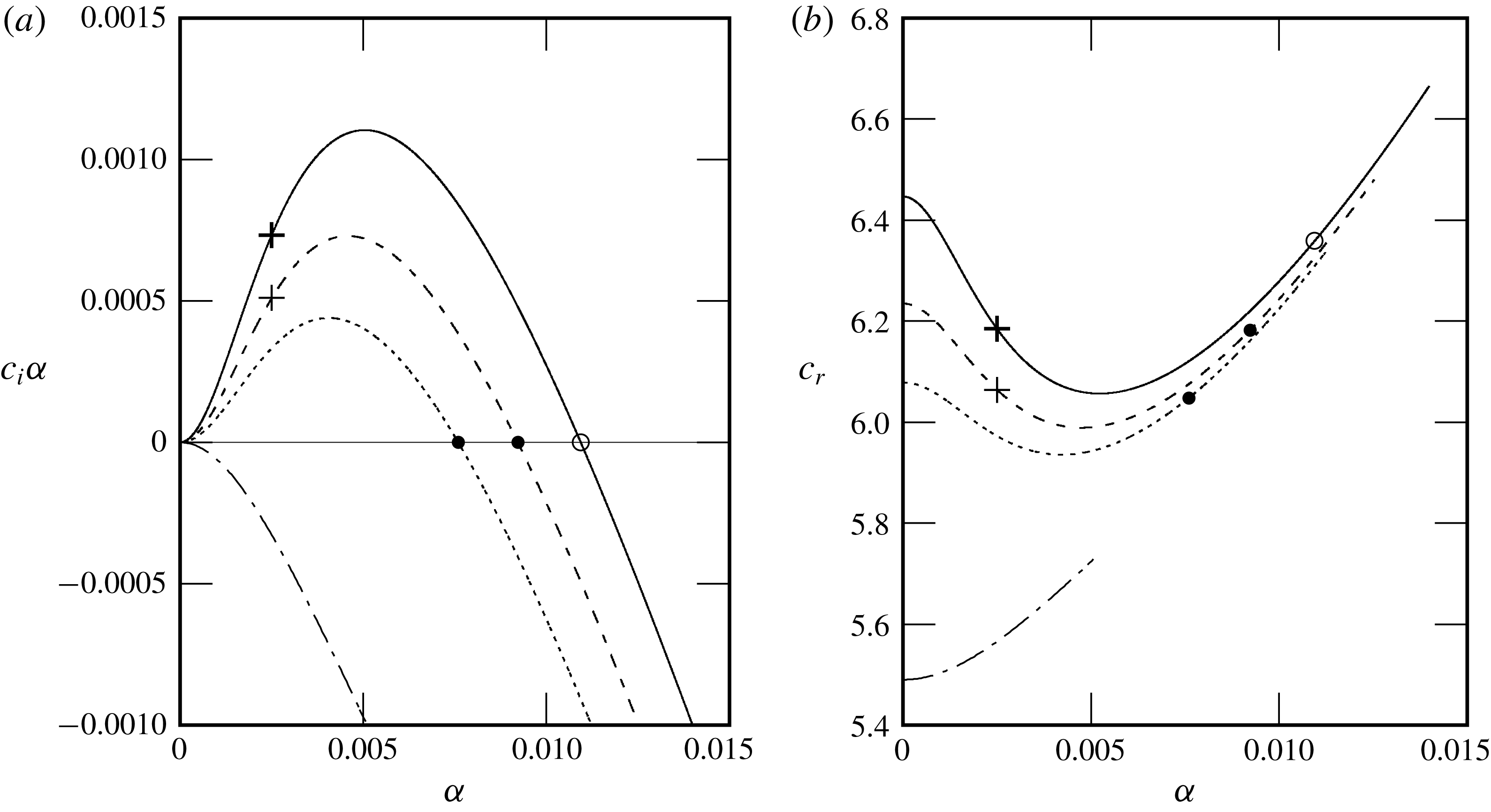
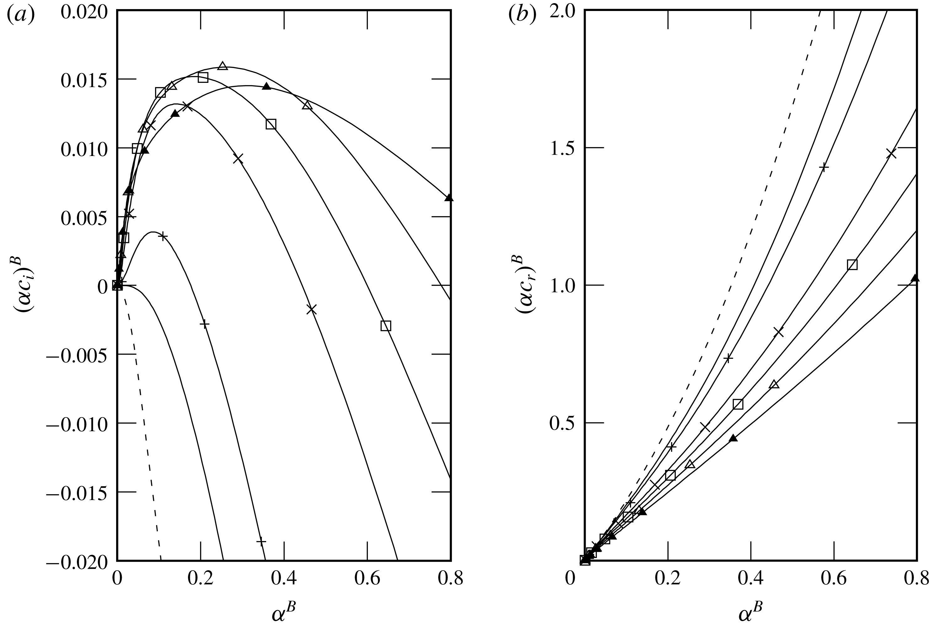
This means that the confinement can fully stabilize the Kapitza instability at a given Reynolds number. We now investigate this suppression of the instability in further detail based on our stability calculations. In figure 11(a), we have plotted the temporal growth rate for a water film at
 $Re_{l}=23.9$
and
 $\unicode[STIX]{x1D6FD}=3^{\circ }$
as a function of the wavenumber
 $\unicode[STIX]{x1D6FC}$
for different values of
 $\unicode[STIX]{x1D702}$
(figure 11(b) represents the corresponding wave celerity
 $c_{r}$
). We see that the unstable range, i.e. where the wavenumber
 $\unicode[STIX]{x1D6FC}$
is smaller than the cutoff value
 $\unicode[STIX]{x1D6FC}_{c}$
(intersection of the curves with
 $c_{i}\unicode[STIX]{x1D6FC}=0$
) decreases with
 $\unicode[STIX]{x1D702}$
and entirely disappears at
 $\unicode[STIX]{x1D702}=2$
. At this point, the Kapitza instability has been fully suppressed.
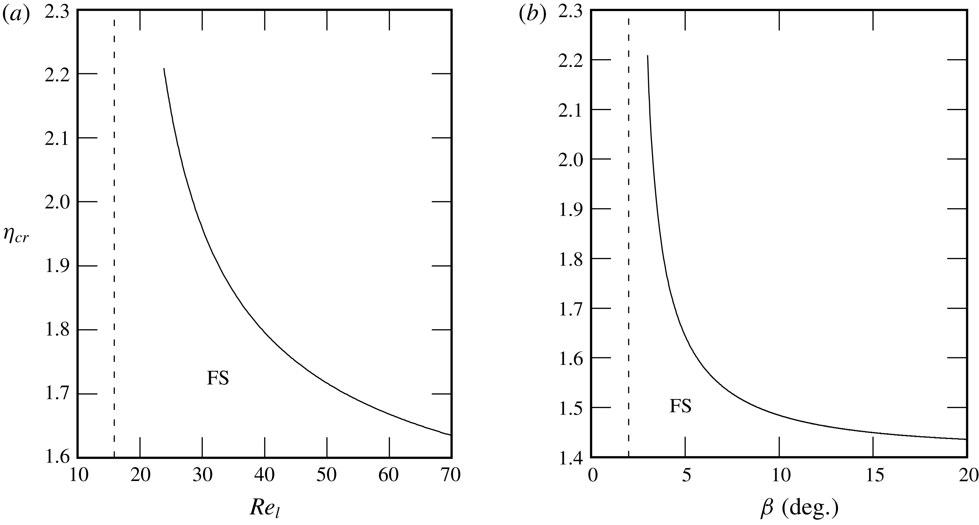
The critical relative confinement
 $\unicode[STIX]{x1D702}_{cr}$
for the suppression of the instability is plotted in figure 12 against the liquid Reynolds number
 $Re_{l}$
(figure 12
a) and the inclination angle
 $\unicode[STIX]{x1D6FD}$
(figure 12
b), respectively. We see that it is easier to suppress the falling film instability the smaller
 $Re_{l}$
and
 $\unicode[STIX]{x1D6FD}$
.
Stability calculations for a water film (
 $Ka=3592$
) at
 $Re_{l}=23.9$
and
 $\unicode[STIX]{x1D6FD}=3^{\circ }$
in contact with aerostatic air. Effect of confinement on (a) temporal growth rate and (b) wave celerity. Solid line, passive-gas limit; dashed line,
 $\unicode[STIX]{x1D702}=3.6$
; dotted line,
 $\unicode[STIX]{x1D702}=2.8$
; dash-dotted line,
 $\unicode[STIX]{x1D702}=2$
. The
 $+$
symbol marks data points that will be discussed in § 5. The filled and open circles correspond to the cutoff wavenumber
 $\unicode[STIX]{x1D6FC}_{c}$
for the confined and passive-gas configurations.

Numerical calculation of the critical confinement
 $\unicode[STIX]{x1D702}_{cr}=\unicode[STIX]{x1D702}(\unicode[STIX]{x1D6FC}_{c}=0)$
below which a water film (
 $Ka=3592$
) in contact with aerostatic air is fully stabilized (FS). (a) Effect of the liquid Reynolds number
 $Re_{l}$
at
 $\unicode[STIX]{x1D6FD}=3^{\circ }$
. The vertical dashed line marks the critical Reynolds number in the passive-gas limit
 $Re_{cr}^{\infty }=(5/6)\cot \unicode[STIX]{x1D6FD}=15.9$
. (b) Effect of the inclination angle
 $\unicode[STIX]{x1D6FD}$
at
 $Re_{l}=23.9$
. The vertical dashed line marks the critical angle in the passive-gas limit
 $\unicode[STIX]{x1D6FD}_{cr}^{\infty }=\arctan ((5/6)/Re_{l})=2^{\circ }$
.

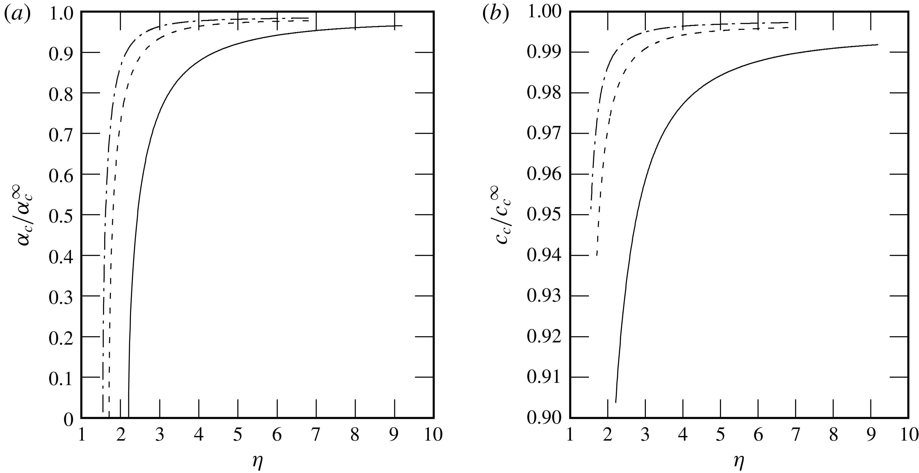
No such curve can be obtained for the remaining control parameter, the Kapitza number
 $Ka$
, as the onset of the long-wave instability is unaffected by surface tension. Instead, we have plotted in figure 13 the cutoff wavenumber (figure 13
a) and the corresponding wave celerity (figure 13
b) as a function of
 $\unicode[STIX]{x1D702}$
for the three studied liquids, which display a substantial variation of
 $Ka$
. In both panels, the plotted quantity is related to its value in the limit of a passive gas. We see that the stabilizing effect of confinement is felt earlier for water (
 $Ka=3592$
) compared to aqueous solutions of DMSO (
 $Ka=509.5$
) and glycerin (
 $Ka=331.8$
). Figure 13(b) shows that the confinement-induced stabilization of the liquid film is accompanied by a decrease of the wave celerity.
Stabilization due to confinement for different working liquids at
 $Re_{l}=23.9$
and
 $\unicode[STIX]{x1D6FD}=3^{\circ }$
in contact with aerostatic air. (a) Cutoff wavenumber and (b) cutoff wave celerity compared to their passive-gas limits
 $\unicode[STIX]{x1D6FC}_{c}^{\infty }$
and
 $c_{c}^{\infty }$
(open circles in figure 11
a,b). Solid line, water (
 $Ka=3592$
); dashed line, aqueous solution of DMSO at
 $83.11\,\%$
by weight (
 $Ka=509.5$
); dash-dotted line, aqueous solution of glycerin at
 $50\,\%$
by weight (
 $Ka=331.8$
).

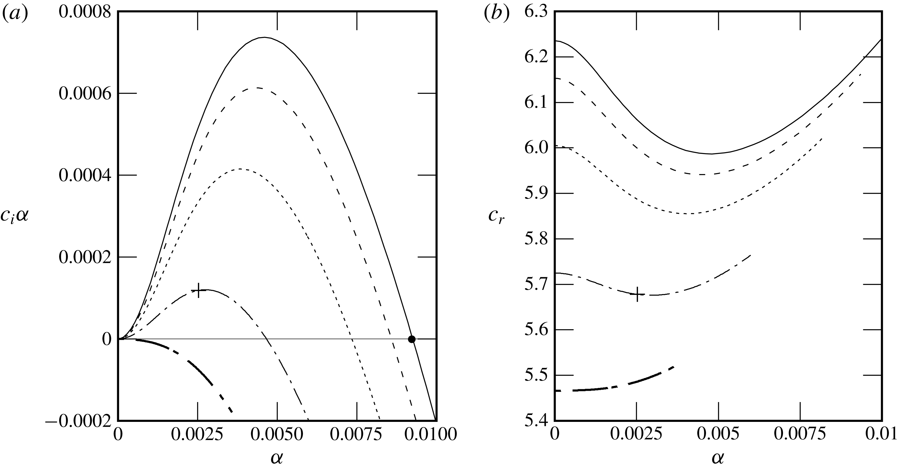
Influence of an increasingly strong counter-current air flow on the stability of a falling water film (
 $Ka=3592$
) at
 $\unicode[STIX]{x1D6FD}=3^{\circ }$
,
 $Re_{l}=23.9$
and
 $\unicode[STIX]{x1D702}=3.6$
. (a) Temporal growth rate; (b) wave celerity. Solid line,
 $M=1$
(
 $Re_{g}=3.0$
); dashed line,
 $M=10$
(
 $Re_{g}=-0.94$
); dotted line,
 $M=25$
(
 $Re_{g}=-7.2$
); dash-dotted line,
 $M=50$
(
 $Re_{g}=-17.1$
); thick dash-dotted line,
 $M=70$
(
 $Re_{g}=-24.4$
). The
 $+$
symbol marks data points that will be discussed in § 5. The filled circle in (a) marks the cutoff wavenumber
 $\unicode[STIX]{x1D6FC}_{c}^{a}$
for the aerostatic configuration.

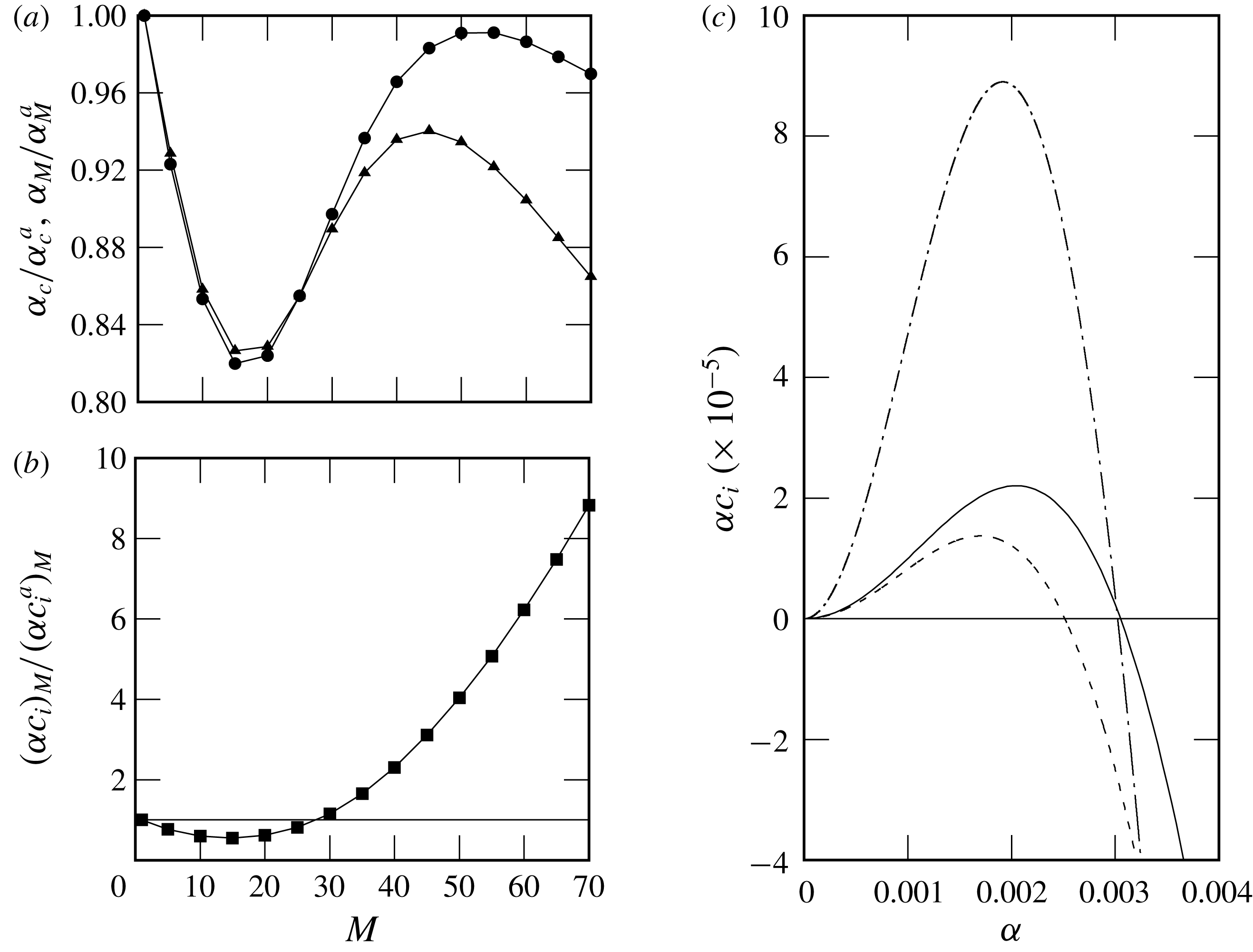
Effect of an increasingly strong counter-current air flow (
 $M=\unicode[STIX]{x0394}p/\unicode[STIX]{x0394}p^{a}$
) on the stability of a falling water film (
 $Ka=3592$
) at
 $\unicode[STIX]{x1D6FD}=3^{\circ }$
and
 $\unicode[STIX]{x1D702}=2.8$
. (a) Deviation of the cutoff wavenumber
 $\unicode[STIX]{x1D6FC}_{c}$
from its aerostatic limit
 $\unicode[STIX]{x1D6FC}_{c}^{a}$
at
 $Re_{l}=23.9$
. (b) Deviation of the critical Reynolds number
 $Re_{cr}$
from its aerostatic limit
 $Re_{cr}^{a}$
. Darker regions correspond to a greater stabilization.

Effect of an increasingly strong counter-current air flow (
 $M=\unicode[STIX]{x0394}p/\unicode[STIX]{x0394}p^{a}$
) on the stability of a falling water film (
 $Ka=3592$
) at
 $\unicode[STIX]{x1D6FD}=3^{\circ }$
,
 $\unicode[STIX]{x1D702}=7$
and
 $Re_{l}=17$
. (a) The deviation of the cutoff wavenumber
 $\unicode[STIX]{x1D6FC}_{c}$
(filled circles) and the most unstable wavenumber
 $\unicode[STIX]{x1D6FC}_{M}$
(filled triangles) from their respective aerostatic limits (superscript a). (b) The deviation of the maximum growth rate
 $(\unicode[STIX]{x1D6FC}c_{i})_{M}$
from the corresponding aerostatic limit
 $(\unicode[STIX]{x1D6FC}c_{i}^{a})_{M}$
. The horizontal solid line denotes
 $(\unicode[STIX]{x1D6FC}c_{i})_{M}=(\unicode[STIX]{x1D6FC}c_{i}^{a})_{M}$
. (c) The temporal growth rate. Solid line,
 $M=1$
(
 $Re_{g}=5.0$
); dashed line,
 $M=20$
(
 $Re_{g}=-67.5$
); dash-dotted line,
 $M=50$
(
 $Re_{g}=-175$
).

4.3 Confined gas phase: counter-current flow
We now investigate how confinement affects the stability of the falling liquid film when it is sheared by a counter-current gas flow. For this, we apply an adverse pressure difference
 $\unicode[STIX]{x0394}p>0$
, which is larger than the aerostatic pressure difference
 $\unicode[STIX]{x0394}p^{a}=\unicode[STIX]{x1D6EC}\sin \unicode[STIX]{x1D6FD}$
. The strength of the gas flow is quantified by the pressure difference ratio
 $M=\unicode[STIX]{x0394}p/\unicode[STIX]{x0394}p^{a}$
.
Figure 14 represents stability calculations for a falling water film at
 $\unicode[STIX]{x1D6FD}=3^{\circ }$
and
 $Re_{l}=23.9$
. The relative confinement is fixed to
 $\unicode[STIX]{x1D702}=3.6$
and the adverse pressure difference is increased. Figure 14(a) shows that increasing the counter-current gas flow increasingly stabilizes the film until the point of fully suppressing the Kapitza instability (thick dash-dotted line). Figure 14(b) shows that this stabilization is accompanied by a decrease in wave celerity.
The level of stabilization strongly depends on the inclination angle
 $\unicode[STIX]{x1D6FD}$
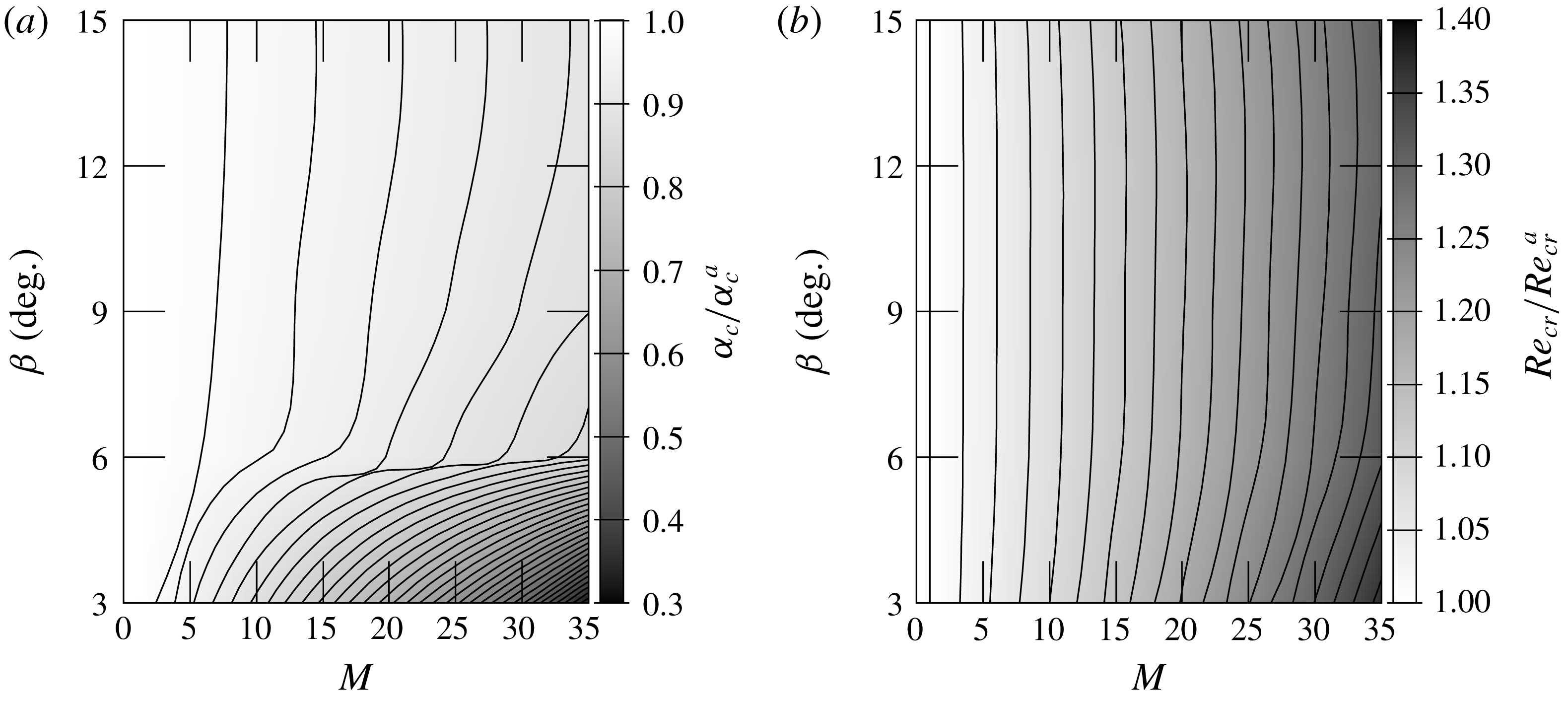
, as shown in figure 15(a,b), which represents contours of the cutoff wavenumber (for
 $Re_{l}=23.9$
) and critical Reynolds number related to their aerostatic limit as a function of
 $\unicode[STIX]{x1D6FD}$
and
 $M$
. At low inclination angles and relatively high adverse pressure gradients, the cutoff wavenumber is reduced by up to
 $70\,\%$
with respect to the aerostatic case and the critical Reynolds number is increased by up to
 $40\,\%$
.
The dispersion curves in figure 14 exhibit a number of features that seem to contradict the stability results of Alekseenko et al. (Reference Alekseenko, Aktershev, Cherdantsev, Kharlamov and Markovich2009), Vellingiri et al. (Reference Vellingiri, Tseluiko and Kalliadasis2015) and Trifonov (Reference Trifonov2017), which were obtained for a weakly confined turbulent gas flow (
 $\unicode[STIX]{x1D702}=24{-}260$
in Trifonov (Reference Trifonov2017)). Firstly, increasing the gas flow reduces monotonically our unstable range of wavenumbers, whereas Vellingiri et al. (Reference Vellingiri, Tseluiko and Kalliadasis2015) and Trifonov (Reference Trifonov2017) found that the cutoff wavenumber can first decrease and then increase with the gas velocity magnitude. Secondly, our growth rate is reduced at all wavenumbers, whereas Alekseenko et al. (Reference Alekseenko, Aktershev, Cherdantsev, Kharlamov and Markovich2009) found that increasing the gas velocity magnitude may reduce the cutoff wavenumber but increase the maximal growth rate at the same time. In that case, long waves are amplified and short waves are stabilized.
It turns out that these differences are due not to the laminar gas flow conditions, but to the strong confinement levels studied here. Indeed, for weaker confinement levels, we recover the same qualitative behaviour as Alekseenko et al. (Reference Alekseenko, Aktershev, Cherdantsev, Kharlamov and Markovich2009), Vellingiri et al. (Reference Vellingiri, Tseluiko and Kalliadasis2015) and Trifonov (Reference Trifonov2017), notwithstanding that the gas flow is laminar in our case. This is shown in figure 16, where we consider a significantly weaker confinement (
 $\unicode[STIX]{x1D702}\geqslant 7$
). Figure 16(a) shows that the cutoff wavenumber (filled circles) now varies non-monotonically with increasing gas flow. Interestingly, this curve displays an additional local maximum in addition to the local minimum reported by Vellingiri et al. (Reference Vellingiri, Tseluiko and Kalliadasis2015) and Trifonov (Reference Trifonov2017). In the same graph, we have also plotted the maximally amplified wavenumber (filled triangles), which varies in the same manner. Figure 16(b) shows the corresponding curve for the maximum growth rate, which displays only a local minimum.
In figure 16(c), we have plotted growth-rate dispersion curves for three representative points from figure 16(a). In contrast to the dispersion curves in figure 14(a) (where
 $\unicode[STIX]{x1D702}=3.6$
), we see that increasing the gas flow can now stabilize short waves while amplifying long waves (compare solid and dot-dashed lines), in accordance with Alekseenko et al. (Reference Alekseenko, Aktershev, Cherdantsev, Kharlamov and Markovich2009). For an even weaker confinement level (
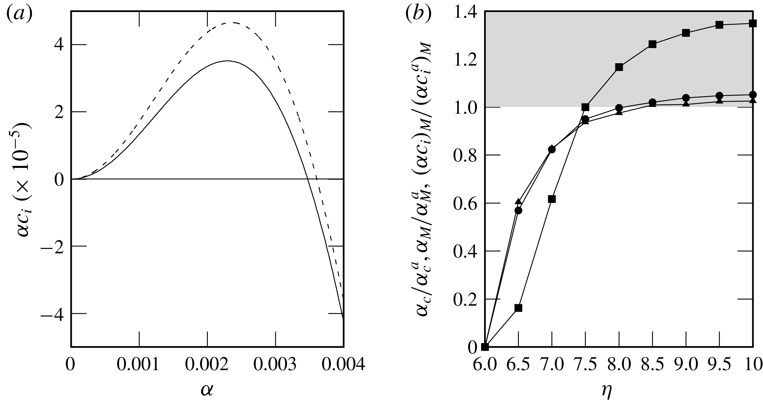
 $\unicode[STIX]{x1D702}=9$
), we find that an increased gas flow can destabilize the film at all wavenumbers, as shown in figure 17(a). Figure 17(b), which plots different characteristic points of the growth-rate dispersion curve as a function of
 $\unicode[STIX]{x1D702}$
, allows one to identify the critical confinement at which this transition occurs (
 $\unicode[STIX]{x1D702}=8$
for
 $Re_{l}=17$
and
 $\unicode[STIX]{x1D6FD}=3^{\circ }$
). Just before the transition (
 $\unicode[STIX]{x1D702}=7.5{-}8$
), the cutoff wavenumber is reduced with respect to the aerostatic limit while the maximum growth rate is increased, similarly to what was observed by Alekseenko et al. (Reference Alekseenko, Aktershev, Cherdantsev, Kharlamov and Markovich2009).
Effect of the relative confinement
 $\unicode[STIX]{x1D702}$
on the stability of a falling water film (
 $Ka=3592$
) at
 $\unicode[STIX]{x1D6FD}=3^{\circ }$
,
 $Re_{l}=17$
and
 $Re_{g}=-67.5$
. (a) The temporal growth rate. Solid line,
 $M=1$
and
 $\unicode[STIX]{x1D702}=9$
; dashed line,
 $Re_{g}=-67.5$
(
 $M=9.1$
) and
 $\unicode[STIX]{x1D702}=9$
. (b) The deviation of the cutoff wavenumber
 $\unicode[STIX]{x1D6FC}_{c}$
(filled circles), most unstable wavenumber
 $\unicode[STIX]{x1D6FC}_{M}$
(filled triangles) and maximum growth rate
 $(\unicode[STIX]{x1D6FC}c_{i})_{M}$
(filled squares) from their respective aerostatic limits. The grey area marks the unstable region compared to the aerostatic scenario.

5 Explanation of the stabilization mechanism
To identify the mechanism responsible for the confinement-induced stabilization of the Kapitza instability, we focus on three representative cases for which linear stability data were reported in § 4 (the two points marked by plus symbols in figure 11 and the single point also marked by a plus symbol in figure 14). In all three cases, we have
 $Re_{l}=23.9$
and
 $\unicode[STIX]{x1D6FD}=3^{\circ }$
, whereas the conditions for the gas differ as follows: (i) aerostatic gas with weak relative confinement
 $\unicode[STIX]{x1D702}=12.4$
; (ii) aerostatic gas with strong relative confinement
 $\unicode[STIX]{x1D702}=3.6$
; and (iii) counter-current gas with
 $Re_{g}=-17.1$
and strong relative confinement
 $\unicode[STIX]{x1D702}=3.6$
.
For each case, we evaluate the linear perturbation of different interfacial quantities based on a representative unstable mode fixed by the wavenumber
 $\unicode[STIX]{x1D6FC}=0.0025$
(situated on the ascending branch of the growth-rate curves in figures 11 and 14). These perturbations can all be expressed in terms of the streamfunction perturbation amplitudes
 $\hat{\unicode[STIX]{x1D719}}$
and
 $\hat{\unicode[STIX]{x1D713}}$
(2.14), which are the eigenfunctions of the Orr–Sommerfeld problem (2.15). For example, the film thickness perturbation
 $h^{\star }$
(2.20) can be written as
 $$\begin{eqnarray}\left.\begin{array}{@{}c@{}}h^{\star }={\hat{h}}\exp [\text{i}\unicode[STIX]{x1D6FC}(x-ct)+\text{i}\unicode[STIX]{x1D6E9}_{h}],\\ \displaystyle {\hat{h}}=\hat{\unicode[STIX]{x1D719}}\,\sqrt{\text{Re}\{1/\text{}\underline{c}\}^{2}+\text{Im}\{1/\text{}\underline{c}\}^{2}},\quad \unicode[STIX]{x1D6E9}_{h}=\arctan [\text{Im}\{1/\text{}\underline{c}\}/\text{Re}\{1/\text{}\underline{c}\}],\end{array}\right\}\end{eqnarray}$$
where
 $\unicode[STIX]{x1D6E9}_{h}$
designates the phase shift with respect to the streamfunction perturbation (2.14a
). Further, we are interested in the perturbed adverse tangential shear stress
 $\unicode[STIX]{x1D70F}_{t}$
exerted by the gas on the film surface,
 $$\begin{eqnarray}\unicode[STIX]{x1D70F}_{t}=T_{t}+\unicode[STIX]{x1D70F}_{t}^{\star },\end{eqnarray}$$
where
 $T_{t}<0$
is the tangential interfacial shear stress of the primary flow and the shear stress perturbation
 $\unicode[STIX]{x1D70F}_{t}^{\star }$
subsumes the two contributions associated with interfacial quantities defined by the last two terms in (2.18):
 $$\begin{eqnarray}\left.\begin{array}{@{}c@{}}\unicode[STIX]{x1D70F}_{t}^{\star }=\hat{\unicode[STIX]{x1D70F}}_{t}\exp [\text{i}\unicode[STIX]{x1D6FC}(x-ct)+\text{i}\unicode[STIX]{x1D6E9}_{\unicode[STIX]{x1D70F}}],\\ \displaystyle \hat{\unicode[STIX]{x1D70F}}_{t}=\sqrt{\text{Re}\{Z_{\unicode[STIX]{x1D70F}}\}^{2}+\text{Im}\{Z_{\unicode[STIX]{x1D70F}}\}^{2}},\quad \unicode[STIX]{x1D6E9}_{\unicode[STIX]{x1D70F}}=\arctan [\text{Im}\{Z_{\unicode[STIX]{x1D70F}}\}/\text{Re}\{Z_{\unicode[STIX]{x1D70F}}\}],\\ \displaystyle Z_{\unicode[STIX]{x1D70F}}={\unicode[STIX]{x1D6F1}_{\unicode[STIX]{x1D70C}}}^{-1}[\hat{\unicode[STIX]{x1D719}}^{\prime \prime }+U_{l}^{\prime \prime }\,\hat{\unicode[STIX]{x1D719}}\text{}\underline{c}^{-1}+\unicode[STIX]{x1D6FC}^{2}\hat{\unicode[STIX]{x1D719}}],\end{array}\right\}\end{eqnarray}$$
where the purely real amplitude
 $\hat{\unicode[STIX]{x1D70F}}_{t}$
of the perturbation and its phase shift
 $\unicode[STIX]{x1D6E9}_{\unicode[STIX]{x1D70F}}$
follow from the complex amplitude
 $Z_{\unicode[STIX]{x1D70F}}$
. Similarly, and with the help of (2.21b
), we obtain for the perturbed interfacial gas pressure
 $p_{g}^{\star }$
:
 $$\begin{eqnarray}\left.\begin{array}{@{}c@{}}p_{g}^{\star }=\hat{p}_{g}\exp [\text{i}\unicode[STIX]{x1D6FC}(x-ct)+\text{i}\unicode[STIX]{x1D6E9}_{p}],\\ \displaystyle \hat{p}_{g}=\sqrt{\text{Re}\{Z_{p}\}^{2}+\text{Im}\{Z_{p}\}^{2}},\quad \unicode[STIX]{x1D6E9}_{p}=\arctan [\text{Im}\{Z_{p}\}/\text{Re}\{Z_{p}\}],\\ \displaystyle Z_{p}=\underbrace{\text{}\underline{c}\,\hat{\unicode[STIX]{x1D713}}^{\prime }+U_{g}^{\prime }\hat{\unicode[STIX]{x1D713}}}_{Z_{p}^{\unicode[STIX]{x1D70C}}}+\underbrace{\unicode[STIX]{x1D6F1}_{\unicode[STIX]{x1D707}}(\text{i}\unicode[STIX]{x1D6FC}\unicode[STIX]{x1D6F1}_{\unicode[STIX]{x1D70C}})^{-1}(\hat{\unicode[STIX]{x1D713}}^{\prime \prime \prime }-\unicode[STIX]{x1D6FC}^{2}\,\hat{\unicode[STIX]{x1D713}}^{\prime })}_{Z_{p}^{\unicode[STIX]{x1D707}}}-\underbrace{\cos \unicode[STIX]{x1D6FD}\,\hat{\unicode[STIX]{x1D719}}\text{}\underline{c}^{-1}}_{Z_{p}^{\unicode[STIX]{x1D6FD}}},\end{array}\right\}\end{eqnarray}$$
where the components
 $Z_{p}^{\unicode[STIX]{x1D70C}}$
and
 $Z_{p}^{\unicode[STIX]{x1D707}}$
of the complex amplitude
 $Z_{p}$
, through (2.21b
), can be traced directly to the inertial and viscous contributions in the streamwise momentum equation, whereas
 $Z_{p}^{\unicode[STIX]{x1D6FD}}$
comes from the last term in (2.18).
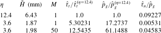
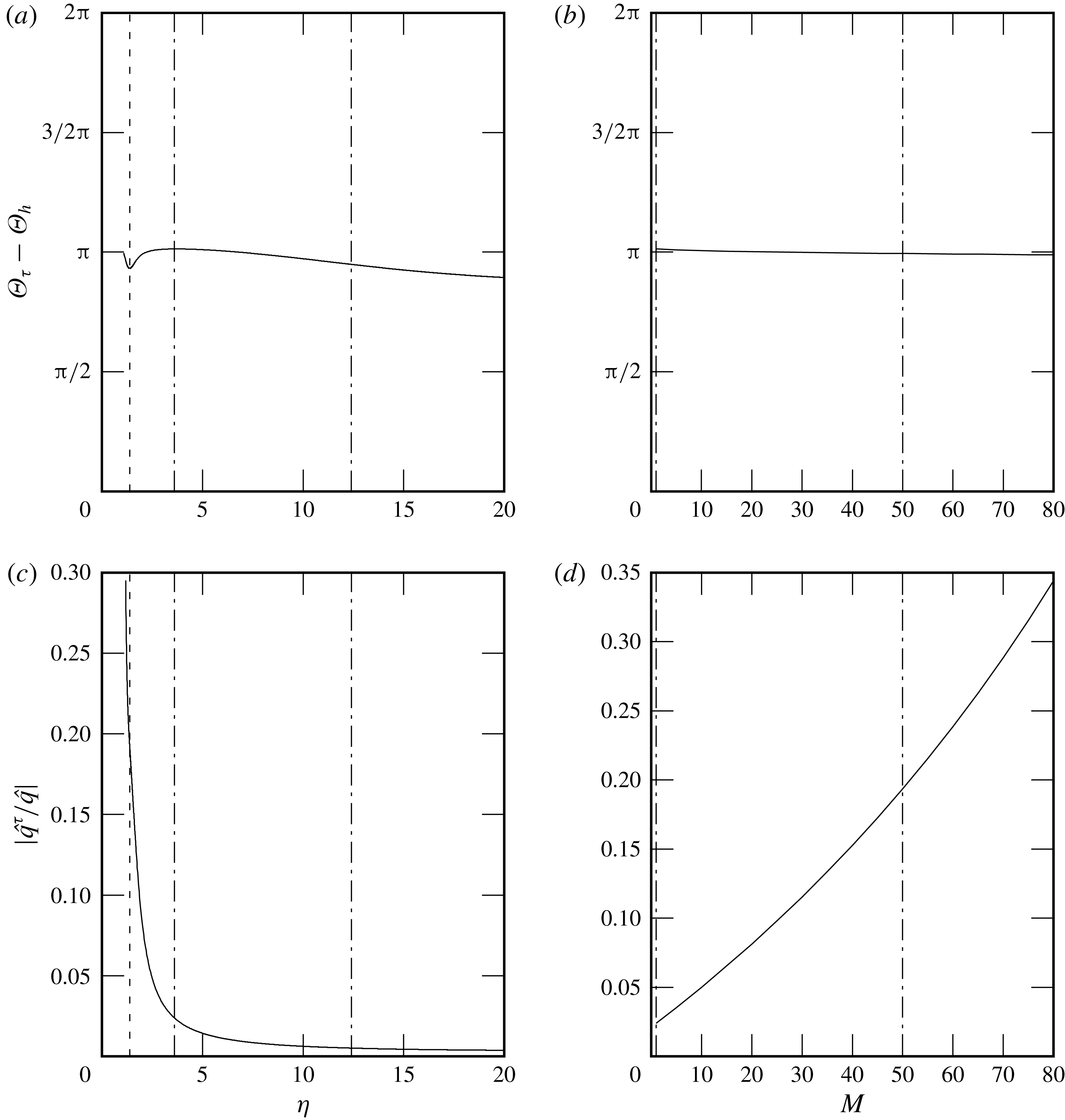
Ratio between the perturbation amplitudes (computed through (2.18)) of the stresses exerted by an air flow on a water film inclined at
 $\unicode[STIX]{x1D6FD}=3^{\circ }$
with
 $Re_{l}=23.9$
: tangential shear stress
 $\hat{\unicode[STIX]{x1D70F}}_{t}$
, static pressure
 $\hat{p}_{g}$
and normal viscous stress
 $\hat{\unicode[STIX]{x1D70F}}_{n}$
. Wavenumber
 $\unicode[STIX]{x1D6FC}=0.0025$
.

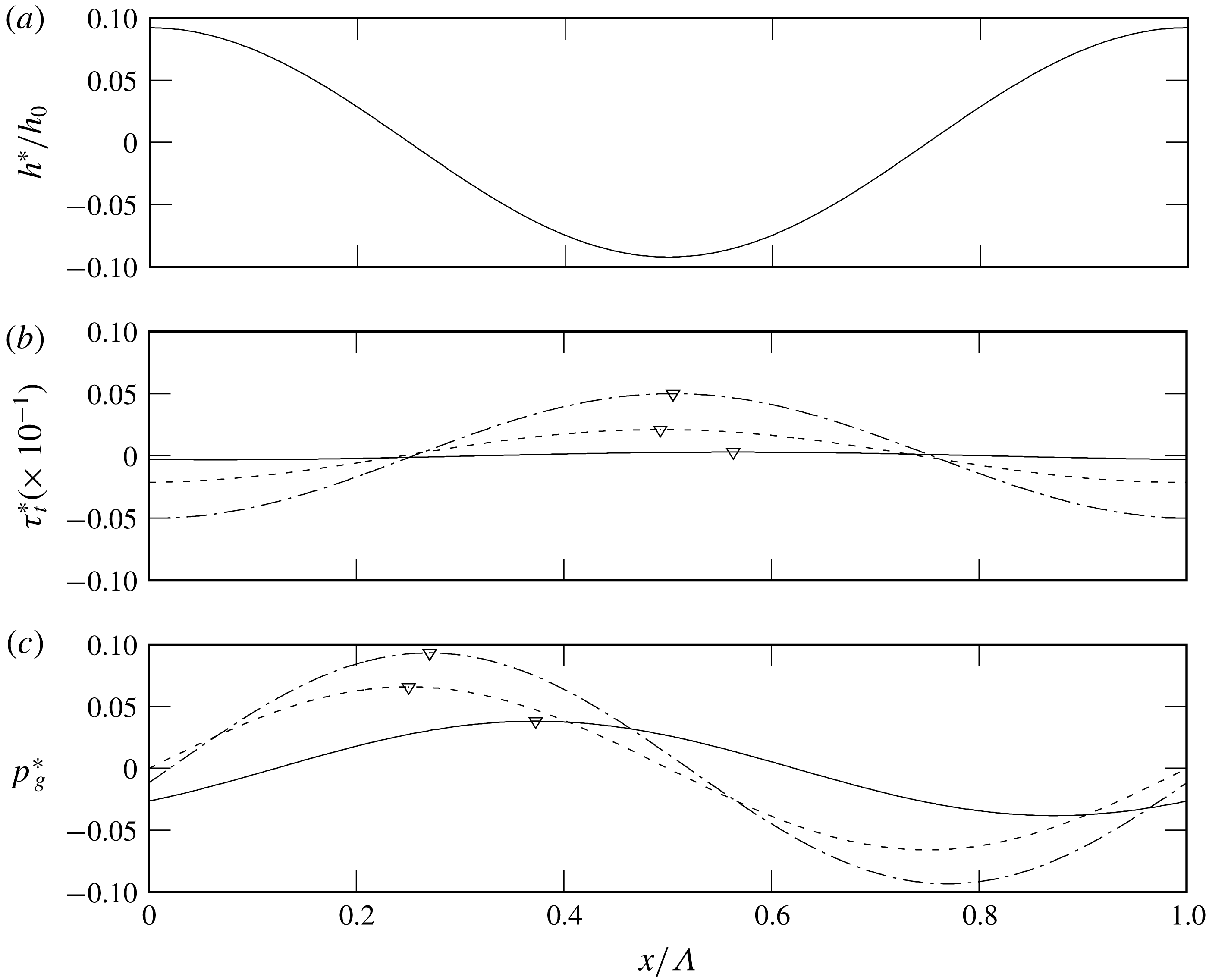
Figure 18(b,c) represent the perturbation profiles of the shear stress (5.3) and pressure (5.4) for the three studied cases, allowing one to discern their phase shifts
 $\unicode[STIX]{x1D6E9}_{\unicode[STIX]{x1D70F}}-\unicode[STIX]{x1D6E9}_{h}$
and
 $\unicode[STIX]{x1D6E9}_{p}-\unicode[STIX]{x1D6E9}_{h}$
with respect to the film thickness perturbation profile (figure 18
a). These profiles have been scaled differently for the three cases, in order to facilitate a comparison within the same graph. The respective perturbation amplitudes
 $\hat{\unicode[STIX]{x1D70F}}_{t}$
and
 $\hat{p}_{g}$
and that of the gas-side normal viscous stress
 $\hat{\unicode[STIX]{x1D70F}}_{n}$
are given in table 5. In addition, table 6 compares the weight of the inertial and viscous contributions to the pressure perturbation’s phase shift
 $\unicode[STIX]{x1D6E9}_{p}$
via the arguments
 $\text{Im}\{Z_{p}^{\unicode[STIX]{x1D70C}}\}/\text{Re}\{Z_{p}\}$
and
 $\text{Im}\{Z_{p}^{\unicode[STIX]{x1D707}}\}/\text{Re}\{Z_{p}\}$
.
From these data, we may conclude that: (i) the perturbation of the normal viscous stress is negligible compared to that of the pressure; (ii) both the perturbation amplitudes
 $\hat{\unicode[STIX]{x1D70F}}_{t}$
and
 $\hat{p}_{g}$
increase with confinement and gas velocity; (iii) for strong confinement, the phase shift with respect to the film thickness perturbation is fixed to
 $\unicode[STIX]{x1D6E9}_{\unicode[STIX]{x1D70F}}-\unicode[STIX]{x1D6E9}_{h}\approx \unicode[STIX]{x03C0}$
for the shear stress perturbation and
 $\unicode[STIX]{x1D6E9}_{p}-\unicode[STIX]{x1D6E9}_{h}\approx \unicode[STIX]{x03C0}/2$
for the pressure perturbation, and this does not change significantly when the gas velocity is increased; and (iv) for strong confinement, the phase shift
 $\unicode[STIX]{x1D6E9}_{p}$
is entirely governed by viscous effects and inertia plays no role.
Water film at
 $\unicode[STIX]{x1D6FD}=3^{\circ }$
: linear perturbations of (a) the film thickness (5.1), (b) the tangential stress (5.3) and (c) the interfacial gas pressure (5.4) associated with a particular eigenmode, i.e.
 $\unicode[STIX]{x1D6FC}=0.0025$
(wavelength
 $\unicode[STIX]{x1D6EC}=2\unicode[STIX]{x03C0}/\unicode[STIX]{x1D6FC}$
). Solid line,
 $\unicode[STIX]{x1D702}=12.4$
aerostatic (
 $M=1$
); dashed line,
 $\unicode[STIX]{x1D702}=3.6$
aerostatic (
 $M=1$
); dash-dotted line,
 $\unicode[STIX]{x1D702}=3.6$
counter-current gas (
 $M=50$
). Triangles in panels (b) and (c) mark the location of the maximum. Pressure perturbations are scaled with different coefficients to facilitate the representation:
 $60$
for
 $\unicode[STIX]{x1D702}=12.4$
;
 $600$
for
 $\unicode[STIX]{x1D702}=3.6$
aerostatic; and
 $1500$
for
 $\unicode[STIX]{x1D702}=3.6$
with
 $M=50$
.


The
 $\unicode[STIX]{x1D6E9}_{p}-\unicode[STIX]{x1D6E9}_{h}\approx \unicode[STIX]{x03C0}/2$
phase shift of the pressure perturbation means that its second derivative
 $\unicode[STIX]{x2202}_{xx}p_{g}^{\star }$
vanishes at the film thickness extrema. As a result, its effect on stability is neutral, i.e. it neither reinforces nor attenuates the film thickness perturbation. This phase shift follows directly from the dominance of viscous effects in the gas flow, i.e.
 $\text{Im}\{Z_{p}^{\unicode[STIX]{x1D707}}\}\gg \text{Im}\{Z_{p}^{\unicode[STIX]{x1D70C}}\}$
. Indeed, in this inertialess limit, the pressure gradient is proportional to one over the third power of the local gas layer thickness (locally developed Poiseuille–Couette flow). Conversely, in the case of inertia-dominated flow, the pressure would be proportional to the square of the local gas velocity (following the Bernoulli equation) and thus its minimum would arise at the maximum of the film thickness perturbation, giving an anti-cyclic (
 $\unicode[STIX]{x1D6E9}_{p}-\unicode[STIX]{x1D6E9}_{h}=\unicode[STIX]{x03C0}$
) phase shift. This would have a destabilizing effect. However, for our case of strongly confined gas flow,
 $\unicode[STIX]{x1D6E9}_{p}-\unicode[STIX]{x1D6E9}_{h}\approx \unicode[STIX]{x03C0}/2$
and the pressure perturbation plays no role in determining the state of stability. This is in agreement with Trifonov (Reference Trifonov2017), who, in his stability analysis, did not find any unstable mode related to the Kelvin–Helmholtz instability for flow conditions similar to those studied here.
Thus, it is the perturbation of the interfacial tangential shear stress that is responsible for the confinement-related stabilization of the falling liquid film, as suggested by Tilley et al. (Reference Tilley, Davis and Bankoff1994). In particular, this results from the
 $\unicode[STIX]{x1D6E9}_{\unicode[STIX]{x1D70F}}-\unicode[STIX]{x1D6E9}_{h}\approx \unicode[STIX]{x03C0}$
phase shift of the shear stress perturbation with respect to the film thickness perturbation
 $h^{\star }$
, which remains virtually unchanged over a wide range of confinement levels and gas velocities (see figure 19
a,b). Owing to this, the adverse tangential shear stress
 $\unicode[STIX]{x1D70F}_{t}$
(5.2) is more negative at the wave hump and less negative at the wave trough. This is principally caused by the change in cross-section for the gas flow, which is smaller above the wave hump and greater above the wave trough.
So, how does the profile of the tangential stress perturbation
 $\unicode[STIX]{x1D70F}_{t}^{\star }$
in figure 18(b) stabilize the film? First, we recall that the driving mechanism of the Kapitza instability is inertia, which causes the liquid flow rate
 $q_{l}(x,t)$
to lag behind its inertialess target value:
 $$\begin{eqnarray}\unicode[STIX]{x1D632}(x,t)=-K_{l}\frac{h^{3}}{3}+\unicode[STIX]{x1D70F}_{t}\frac{h^{2}}{2},\end{eqnarray}$$
where
 $K_{l}$
is defined in (2.9a
). Just upstream of the wave hump, where
 $\unicode[STIX]{x1D632}$
decreases in time as the wave passes by, the actual flow rate
 $q_{l}$
is slightly too high, while it is slightly too low just downstream of the hump, where
 $\unicode[STIX]{x1D632}$
increases in time. The resulting discrepancy in flow into and out of the hump causes it to grow. The effect is stronger the more the actual flow rate
 $q_{l}$
lags behind its target value
 $\unicode[STIX]{x1D632}$
, and that depends on how steeply
 $\unicode[STIX]{x1D632}$
changes within the wavy film.
According to (5.5), the effect of gravity (through the
 $h^{3}$
term in (5.5)) tends to increase variations in
 $\unicode[STIX]{x1D632}$
between the wave hump and wave trough as a result of the change in film thickness
 $h$
. The adverse tangential interfacial stress
 $\unicode[STIX]{x1D70F}_{t}$
, through its perturbation
 $\unicode[STIX]{x1D70F}_{t}^{\star }$
(figure 18
b), counteracts this effect. Indeed,
 $\unicode[STIX]{x1D70F}_{t}^{\star }$
acts to homogenize the flow rate within the film, slowing the flow in the wave hump to a greater extent than underneath the wave trough. This is a direct result of the phase lag observed between the film thickness and the shear stress perturbation (figure 18), and the effect increases with the relevance of the second term in (5.5).
We quantify this by considering the linear perturbation amplitude of the inertialess flow rate (5.5) and by evaluating the contributions due to gravity
 $\hat{\unicode[STIX]{x1D632}}^{g}$
(actually, this term also subsumes the effect of pressure) and shear stress
 $\hat{\unicode[STIX]{x1D632}}^{\unicode[STIX]{x1D70F}}$
:
 $$\begin{eqnarray}\hat{\unicode[STIX]{x1D632}}=\underbrace{-K_{l}h_{0}^{2}{\hat{h}}}_{\hat{\unicode[STIX]{x1D632}}^{g}}+\underbrace{{\textstyle \frac{1}{2}}h_{0}^{2}\hat{\unicode[STIX]{x1D70F}}_{t}+h_{0}T_{t}{\hat{h}}}_{\hat{\unicode[STIX]{x1D632}}^{\unicode[STIX]{x1D70F}}}.\end{eqnarray}$$
Figure 19(c,d) show that the ratio
 $|\hat{\unicode[STIX]{x1D632}}^{\unicode[STIX]{x1D70F}}/\hat{\unicode[STIX]{x1D632}}|$
increases with confinement and gas velocity, which is in accordance with the increase in stabilization observed in figures 11 and 14.
The tangential shear stress also produces an indirect stabilizing effect. It is known that an adverse interfacial shear stress diminishes the celerity
 $c$
of surface waves travelling on falling films (Alekseenko et al.
Reference Alekseenko, Aktershev, Cherdantsev, Kharlamov and Markovich2009; Samanta Reference Samanta2014). This can be explicitly shown in the limit of infinitely long waves (
 $\unicode[STIX]{x1D6FC}\rightarrow 0$
):
 $$\begin{eqnarray}c|_{\unicode[STIX]{x1D6FC}\rightarrow 0}=-K_{l}h_{0}^{2}+T_{t}h_{0}.\end{eqnarray}$$
The wave celerity
 $c$
determines how fast the flow rate within the film would change in the inertialess limit as a wave passes by and reducing it weakens the inertial instability mechanism. In our stability results (figures 11
b and 14
b), we have observed
 $c$
to diminish with increasing confinement and gas velocity, coinciding with an increased stabilization of the film.
Water film at
 $\unicode[STIX]{x1D6FD}=3^{\circ }$
. Phase lag
 $\unicode[STIX]{x1D6E9}_{\unicode[STIX]{x1D70F}}-\unicode[STIX]{x1D6E9}_{h}$
of the perturbations of the film thickness and interfacial tangential shear stress: (a) variation with
 $\unicode[STIX]{x1D702}$
with aerostatic gas (
 $M=1$
); (b) variation with
 $M$
at
 $\tilde{H}=1.87~\text{mm}$
(
 $\unicode[STIX]{x1D702}=3.3{-}3.6$
). Contribution of the interfacial tangential shear stress to the inertialess flow rate (5.6): (c) variation with
 $\unicode[STIX]{x1D702}$
under aerostatic gas (
 $M=1$
); (d) variation with
 $M$
at
 $\tilde{H}=1.87~\text{mm}$
(
 $\unicode[STIX]{x1D702}=3.3{-}3.6$
). The vertical dash-dotted lines mark the three cases represented in figure 18; the vertical dashed line in (a) and (c) marks
 $c_{r}=U|_{h_{0}}$
.

6 Conclusion
Using linear stability calculations and experiments, we have revisited the stability of a falling liquid film flowing down an incline in interaction with a strongly confined laminar gas flow and subject to the Kapitza instability. The gas is either subject to an aerostatic pressure gradient or flows counter-currently.
Tilley et al. (Reference Tilley, Davis and Bankoff1994) suggested that confining the gas phase should stabilize the Kapitza instability, but concluded that this effect is small for water films in contact with air in the studied parameter range. For the same fluid combination, we have found a parameter range where the confinement-related stabilization is very strong, up to the point of suppressing the Kapitza instability altogether. We have shown that the stabilizing effect of confinement is stronger when the inclination is small (
 $\unicode[STIX]{x1D6FD}=1^{\circ }{-}8^{\circ }$
) and/or the Reynolds number is small, and we have determined the critical confinement necessary to fully stabilize the film as a function of these two parameters (figure 12). For example, a water film of
 $0.5~\text{mm}$
thickness flowing down a wall inclined at
 $3^{\circ }$
can be fully stabilized by placing a confining plate at a distance of
 $1~\text{mm}$
from the incline. Water films, which have a high Kapitza number, are found to feel the confinement-induced stabilization earlier than other working fluids with lower Kapitza number, such as aqueous solutions of glycerin or DMSO. The suppression of the Kapitza instability is observed both when the gas is subject to an aerostatic pressure gradient and when it flows counter-currently.
In the latter case, at the strong confinement levels we have focused on, the stabilization is monotonically intensified with increasing gas flow velocity and occurs over the entire range of unstable wavenumbers. This is different from observations by Alekseenko et al. (Reference Alekseenko, Aktershev, Cherdantsev, Kharlamov and Markovich2009), Vellingiri et al. (Reference Vellingiri, Tseluiko and Kalliadasis2015) and Trifonov (Reference Trifonov2017), who found a non-monotonic effect of the gas velocity and an only partial destabilization of the wave spectrum for weakly confined turbulent gas flows. We have recovered these results also for the laminar gas flow conditions considered here, when reducing the confinement level. In this context, we have identified a confinement threshold above which the gas destabilizes the film at all wavenumbers (see figure 17).
We have identified the mechanism responsible for the instability suppression. As suggested by Tilley et al. (Reference Tilley, Davis and Bankoff1994), viscous stresses in the gas play a decisive role. In particular, it is the tangential viscous stress exerted by the gas on the film surface that is decisive. The key of the stabilization mechanism is that there is a phase shift of almost exactly half a wavelength between the film thickness perturbation and the associated shear stress perturbation. Consequently, the adverse shear stress is greater at a wave hump than at a wave trough. This tends to homogenize the local equilibrium flow rate within the liquid film, thus counteracting the effect of gravity, which acts to force larger flow rates where the film is thick (wave hump) and smaller ones where the film is thin (wave trough). As a result, the inertia-related lag between the actual local flow rate and its equilibrium value is reduced and this weakens the inertia-driven mechanism of the Kapitza instability.
Comparison of (a) temporal growth rate and (b) angular wave frequency between our work and Brevdo et al. (Reference Brevdo, Laure, Dias and Bridges1999, figure 2 there). Parameter values:
 $\unicode[STIX]{x1D6FD}=4.6^{\circ }$
,
 $\unicode[STIX]{x1D708}_{l}=5.02\times 10^{-6}$
m
 $^{2}$
s
 $^{-1}$
,
 $\unicode[STIX]{x1D6FE}=69\times 10^{-3}$
N m
 $^{-1}$
,
 $\unicode[STIX]{x1D70C}_{l}=1130$
kg m
 $^{-3}$
,
 $Ka=\unicode[STIX]{x1D6FE}(\unicode[STIX]{x1D70C}_{l}g^{1/3}\unicode[STIX]{x1D708}_{l}^{4/3})^{-1}=331.85$
. Values of the Reynolds number
 $Re^{B}=(3/2)Re_{l}$
:
 $10$
(dashed line),
 $Re_{cr}^{B}=(5/4)\cot \unicode[STIX]{x1D6FD}$
(bare solid line),
 $20$
(pluses),
 $40$
(crosses),
 $60$
(empty squares),
 $100$
(empty triangles),
 $200$
(filled triangles). Note that
 $\unicode[STIX]{x1D6FC}^{B}$
,
 $(\unicode[STIX]{x1D6FC}c_{r})^{B}$
and
 $(\unicode[STIX]{x1D6FC}c_{i})^{B}$
are scaled as in Brevdo et al. (Reference Brevdo, Laure, Dias and Bridges1999), i.e. using the Nusselt film thickness and the free-surface velocity as length and velocity scales.

The stabilization mechanism increases whenever the contribution of the interfacial shear stress in the equilibrium flow rate becomes stronger with respect to that of gravity (and pressure). This is the case when the inclination is weak, the film is thin (
 $Re_{l}$
is small) and the counter-current gas flow is strong. It is under those conditions that our stability calculations and experiments display the strongest stabilization.
We point out that confining the gas phase also contributes to the observed stabilization through an indirect effect, i.e. by reducing the wave celerity. Reducing the wave speed reduces inertia-induced flow-rate imbalances within the liquid film, which again weakens the Kapitza instability.
Acknowledgements
This work was supported by the ANR wavyFILM project, grant ANR-15-CE06-0016-01 of the French Agence Nationale de la Recherche.
Appendix A. Numerical validation of the stability code
To validate our two-phase linear stability code numerically, we have compared its predictions to data from the literature for three examples of interfacial instability.
Figure 20 compares our stability calculations with landmark calculations of Brevdo et al. (Reference Brevdo, Laure, Dias and Bridges1999) for the case of an inclined liquid film falling in a passive atmosphere. We point out that the conditions studied by Brevdo et al. (Reference Brevdo, Laure, Dias and Bridges1999) concern a liquid film flowing in a passive atmosphere (
 $\unicode[STIX]{x1D6F1}_{\unicode[STIX]{x1D707}}=\unicode[STIX]{x1D6F1}_{\unicode[STIX]{x1D70C}}=0$
), whereas in the present work we have considered an active phase.
Figure 21 presents the neutral stability diagram for the long-wave Yih instability (horizontal pressure-driven two-layer flow with
 $\unicode[STIX]{x1D6F1}_{\unicode[STIX]{x1D70C}}=1$
) as obtained by Yiantsios & Higgins (Reference Yiantsios and Higgins1989), in comparison with our calculations (circles).
Neutral stability diagram for a horizontal pressure-driven two-layer flow with
 $\unicode[STIX]{x1D6F1}_{\unicode[STIX]{x1D70C}}=1$
: comparison of our numerical results (circles) with figure 2b of Yiantsios & Higgins (Reference Yiantsios and Higgins1989) (lines). Stable regions are denoted by
 $S$
, unstable regions by
 $U$
.

Finally, table 7 compares our stability data to those of Yiantsios & Higgins (Reference Yiantsios and Higgins1988) and Tilley et al. (Reference Tilley, Davis and Bankoff1994) for a pressure-driven two-layer flow through a horizontal channel, in the absence of gravity. In addition to the numerical punctual values of table 7, we also present in figure 22 the real and imaginary parts of the wave celerity as a function of the wavenumber for the case at
 $Q^{T}=1.6$
and
 $We^{T}=0.2$
(fourth and seventh rows of table 7).
Real and imaginary parts of the wave celerity
 $c$
:
 $\unicode[STIX]{x1D6F1}_{\unicode[STIX]{x1D707}}=1/5$
,
 $\unicode[STIX]{x1D6F1}_{\unicode[STIX]{x1D70C}}=1$
and
 $\unicode[STIX]{x1D702}=2$
. Comparison between our work and results of Yiantsios & Higgins (Reference Yiantsios and Higgins1988, table I there) and Tilley et al. (Reference Tilley, Davis and Bankoff1994, table I there). Scales used in Tilley et al. (Reference Tilley, Davis and Bankoff1994) are related to ours as
 $\unicode[STIX]{x1D6FC}^{\text{T}}=\unicode[STIX]{x1D6FC}H{\mathcal{L}}^{-1}$
,
 $(c_{r},c_{i})^{\text{T}}=(c_{r},c_{i})H{\mathcal{L}}^{-1}$
,
 $Q^{\text{T}}=Re_{l}+Re_{g}$
,
 $We^{\text{T}}=WeH{\mathcal{L}}^{-1}$
.

(a) Real and (b) imaginary wave celerity
 $c$
as a function of the wavenumber:
 $\unicode[STIX]{x1D6F1}_{\unicode[STIX]{x1D707}}=1/5$
,
 $\unicode[STIX]{x1D6F1}_{\unicode[STIX]{x1D70C}}=1$
,
 $\unicode[STIX]{x1D702}=2$
,
 $Q^{\text{T}}=1.6$
and
 $We^{\text{T}}=0.2$
(same parameters as the fourth and seventh rows of table 7, whose numerical values corresponding to our calculations are marked with filled circles). Scales used in Tilley et al. (Reference Tilley, Davis and Bankoff1994) are related to ours as
 $\unicode[STIX]{x1D6FC}^{\text{T}}=\unicode[STIX]{x1D6FC}H{\mathcal{L}}^{-1}$
,
 $(c_{r},c_{i})^{\text{T}}=(c_{r},c_{i})H{\mathcal{L}}^{-1}$
,
 $Q^{\text{T}}=Re_{l}+Re_{g}$
,
 $We^{\text{T}}=WeH{\mathcal{L}}^{-1}$
.

Appendix B. Sensitivity of the comparison in figure 8 with respect to the inclination angle
 $\unicode[STIX]{x1D6FD}$

To remedy the insufficient resolution of the inclinometer, the inclination angle
 $\unicode[STIX]{x1D6FD}$
of the experimental set-up was obtained by fine-tuning (within the precision range
 $\pm 0.05^{\circ }$
of the inclinometer) the value of
 $\unicode[STIX]{x1D6FD}$
in the numerical calculation of the neutral stability curve for the unconfined case, until this matched with the corresponding experimental curve. Figure 8 shows the best match of these curves for one set of conditions, obtained for an inclination angle of
 $\unicode[STIX]{x1D6FD}=1.69^{\circ }$
.
To demonstrate the sensitivity of this comparison with respect to the inclination angle, figure 23 shows this comparison for two slightly different values of
 $\unicode[STIX]{x1D6FD}$
, i.e.
 $\unicode[STIX]{x1D6FD}=1.68^{\circ }$
(a) and
 $\unicode[STIX]{x1D6FD}=1.70^{\circ }$
(b).
Sensitivity of the comparison in figure 8 with respect to the assumed inclination angle
 $\unicode[STIX]{x1D6FD}$
: (a)
 $\unicode[STIX]{x1D6FD}=1.68^{\circ }$
; (b)
 $\unicode[STIX]{x1D6FD}=1.70^{\circ }$
.

Appendix C. Measured streamwise evolution of the wave amplitude
Figure 24 shows the measured streamwise evolution of the wave amplitude along the channel for the ‘unconfined’ (figure 4
b) and the confined (figure 4
a) configurations at
 $Re_{l}=38.7$
, for the same inlet forcing amplitude and frequency. The film is unstable in both cases. The decrease of the wave amplitude induced by strengthening the confinement (changing
 $\unicode[STIX]{x1D702}=22$
to
 $\unicode[STIX]{x1D702}=6.65$
) is approximately 7 %.
Experimental streamwise evolution of the wave amplitude for a water film at
 $Re_{l}=38.7$
and
 $\unicode[STIX]{x1D6FD}=1.69^{\circ }$
with aerostatic air. Open triangles, confined (
 $\unicode[STIX]{x1D702}=6.65$
); filled circles, ‘unconfined’ (
 $\unicode[STIX]{x1D702}=22$
). Forcing frequency
 $\tilde{f}=3.6~\text{Hz}$
.