

1. Introduction
How has the biodiversity agenda evolved during the lifetime of Environment and Development Economics (EDE)? Two decades ago, Perrings et al. (Reference Perrings, Folke and Maler1992) published their assessment of priorities in the biodiversity research agenda given the state of the art at that time. Using their conclusions as a baseline, this paper assesses how the agenda has evolved in response to developments in biodiversity science and policy since that time, paying special attention to changes that affect the developing countries. To anticipate, there have been several main trends in the economics of biodiversity since the early 1990s.
First, biodiversity change has come to be analyzed largely through its impact on ecosystem services – the benefits to humans of ecosystems. Emphasis has shifted from the conservation of endangered species for the sake of conservation to the role of biodiversity in the production of a range of ecosystem services. Increasingly, conservation priorities are motivated by the cost – in terms of the foregone benefits that people derive from the system – of biodiversity loss. This includes benefits deriving from a sense of moral stewardship toward other species but is not limited to that. It also includes: a) the production of foods, fuels, fibers, water, genetic resources, and chemical compounds; b) human, animal, and plant health benefits; c) recreation, renewal, aesthetic, and spiritual satisfaction; and d) the buffering of many ecological processes and functions against the effects of environmental variation.
Second, there has been a growing appreciation that the diversity of species is a source not just of benefits but also of costs. Many of the benefits that people derive from ecosystems depend upon reducing the abundance of pests, predators, pathogens, and competitors. HIV AIDS and SARS, smallpox and rinderpest have a different impact on human well being than the panda, the bald eagle, the ring-tailed lemur, or the giant redwood. Along with this has come a deeper understanding of the factors behind actions that reduce the diversity of species, and the tradeoffs involved in conservation decisions.
Third, while much research still focuses on habitat conversion driven by population and economic growth as the primary drivers of biodiversity change, there is growing awareness that other factors are important. Climate change and the closer integration of the global economic system are recognized as major drivers of biodiversity change. Both are altering not only the abundance but also the distribution of species across the planet. At the same time, we have a deeper understanding of the effects of economic growth on biodiversity. Although evidence on the link between poverty and environmental change generally remains mixed, it has become increasingly clear that the loss of many genera is a seemingly unavoidable cost of income growth in the least-developed economies.
Fourth, although work on traditional policy instruments to internalize the biodiversity externalities continues, there has been growing interest in the development of instruments to deal with the transboundary public good aspect that characterizes many biodiversity issues. This includes both the design of institutions for the governance of biodiversity as a transboundary public good and the development of mechanisms such as systems of payments for ecosystem services (PES) that change the payoff to local conservation, production or pest control decisions in developing countries that yield wider benefits.
Of these, only the importance of ecosystem services was fully anticipated two decades ago. Perrings et al. (Reference Perrings, Folke and Maler1992) began their review with the statement:
In our opinion the greater part of the biodiversity problem concerns the relation between biodiversity and the ecological services obtained from the biosphere by humanity. The problem here is to maintain that level of biodiversity, which will guarantee the resilience of ecosystems on which not only human consumption and production but also existence depends.
They argued that the value of biological resources, like that of other inputs, derives from the value of the goods and services they produce. Moreover, the value of biodiversity, the mix of species, derives both from the complementarity and substitutability between species as inputs in the production of ecosystem services, and from a portfolio effect on production risks. In particular, they argued the importance of maintaining sufficient biodiversity to protect the resilience of ecological systems – their capacity to function over a range of environmental conditions. Both arguments are reflected in the literature since that time.
The other trends that have characterized the literature on the economics of biodiversity over the last two decades have been stimulated by developments both in the science of biodiversity and in the governance of global environmental resources. The deepening understanding of climate change has fundamentally altered the landscape of both environmental science and environmental economics. At the same time the growing focus on microbial communities in biology – and especially on zoonoses and pathogens more generally – has altered the landscape of biodiversity science and biodiversity economics. These trends have had a profound effect on what is being studied.
In this paper, I consider how the field has evolved over the life of EDE. It is an appropriate moment to be doing this. The international community has recently agreed to establish an Intergovernmental Science-Policy Platform on Biodiversity and Ecosystem Services (IPBES) to monitor changes in the biosphere with potential implications for human well being. At the heart of the issues involved are the tensions between the multiple roles of biodiversity – the fact that there are tradeoffs between the conservation, production, and biosecurity agendas. Environmental, resource, and ecological economics have a fundamental role to play in elucidating the nature of those tradeoffs and the social opportunity cost of the options under consideration.
2. Biodiversity, production, and conservation
Perhaps the most profound change in the field has been the emergence of ecosystem services as the primary motivation for the conservation of biodiversity. The Convention on Biological Diversity (Reference Convention on Biological Diversity1993) was conceptualized as an agreement to secure both conservation and the sustainable use of biodiversity. In practice, however, it has interpreted sustainable use rather narrowly to mean the sustainable use of genetic resources. The publication of the Millennium Ecosystem Assessment (Reference Millennium Ecosystem Assessment2005) made it clear that the array of services supported by biodiversity extend well beyond production of the genetic material embodied in distinct species. The Millennium Ecosystem Assessment (MA) defined ecosystem services to include the full array of benefits people obtain from ecosystems, distinguishing four broad benefit streams: the provisioning, cultural, regulating, and supporting services.
The MA defined the provisioning services to include the products of renewable biotic resources including foods, fibers, fuels, water, biochemicals, medicines, pharmaceuticals, as well as the genetic resources of interest to the Convention on Biological Diversity (CBD). Some of these products are directly consumed and are subject to well-defined property rights, implying that they are priced in the market. Others are not. It defined cultural services to include a range of largely nonconsumptive uses of the environment including: (a) the spiritual, religious, aesthetic, and inspirational benefits that people derive from the ‘natural’ world; (b) the value to science of the opportunity to study and learn from that world; and (c) the market benefits of recreation and tourism. The supporting services comprise the main ecosystem processes that underpin all other services, such as soil formation, photosynthesis, primary production, nutrient, carbon, and water cycling. These services play out at very different spatial and temporal scales, extending from the local to the global, and over time periods that range from seconds to hundreds of years. Finally, the regulating services were defined to include air quality regulation, climate regulation, hydrological regulation, erosion regulation or soil stabilization, water purification and waste treatment, disease regulation, pest regulation, and natural hazard regulation.
Even though the end product of many provisioning services is a particular commodity – grain, meat, water, fuel, medicine – the MA underscored the fact that their production depends on a combination of biotic and abiotic inputs. In particular, variability in the supply of provisioning services depends on the role of biodiversity in moderating the effects of environmental variation. In fact, this role of biodiversity defines the regulating services. They limit the effect of stresses and shocks to the system. As with the supporting services they operate at widely differing spatial and temporal scales. So, for example, the morphological variety of plants in an alpine meadow offers strictly local benefits in terms of reduced soil erosion, while the genetic diversity of crops in global agriculture offers a global benefit in terms of a lower spatial correlation of the risks posed by climate or disease.
From an economic perspective, the fact that biodiversity is valued through its role in providing an array of ecosystem services has two main implications. The first is that the value of biodiversity derives from the value of the final goods and services it produces. Biodiversity is treated as an input into the production of these final goods and services. The second is that this requires specification of production functions that embed the ecosystem processes and ecological functions that connect biodiversity and ecosystem services.
This has posed significant challenges to both ecological and economic science. While the last two decades have seen real advances in understanding of biodiversity-ecological functioning-ecosystem services relationships, this is still very much work in progress. Vitousek and Hooper's (Reference Vitousek, Hooper, Schulze and Mooney1993) speculative projection of the impact on ecological functioning of biodiversity loss has stimulated a whole new field of ecology, many of the results of which are reported in Loreau et al. (Reference Loreau, Naeem and Inchausti2002) and Naeem et al. (Reference Naeem, Bunker, Hector, Loreau and Perrings2009). It has led to a deeper understanding of the role of species in ecological functioning, and the relation between ecological functioning and the production of ecosystem services. Species are related through functional traits that make them more or less ‘redundant’ in executing particular ecological functions. Individual species are highly redundant (near perfect functional substitutes for other species) if they share a full set of traits with those other species, Conversely, they are ‘singular’ if they possess a unique set of traits (Naeem, Reference Naeem1998). Species are also related through ecological interactions – trophic relationships, competition, parasitism, facilitation, and so on – that make them more or less complementary in executing ecological functions (Thebault and Loreau, Reference Thebault and Loreau2006).
Understanding the value of species that support particular ecological functions requires an understanding of both their substitutability and complementarity in the performance of these functions. It also requires an understanding of the way in which the simplification of ecosystems for agriculture, forestry, fisheries, etc. affects both the functions they perform and the interactions between functions. The simplification of agroecosystems to privilege particular crops or livestock strains necessarily affects the array of services that system delivers, partly because the number of functions performed increases with the number of species (Hector and Bagchi, Reference Hector and Bagchi2007), and partly because each species in a system typically performs multiple functions (Díaz et al., Reference Díaz, Lavorel, Bello, Quétier, Grigulis and Robson2007). Ecosystems are systems of ‘joint production’. Individual systems generate multiple services. It follows that part of the cost of simplification is the ecosystem services foregone as a result. Industrial agriculture has significantly increased yields per hectare, but it has also significantly reduced a range of other ecosystem services including water supply, water quality, habitat provision, pollination, and soil erosion control (Millennium Ecosystem Assessment, Reference Millennium Ecosystem Assessment2005).
Superimposing the commodity-specific production functions that relate output of marketed commodities to both marketed inputs and the underlying ecological processes adds another layer of complexity. Not surprisingly, the specification and estimation of ecological-economic production functions that capture both the jointness of the production of ecosystem services, the interactions between services, and the impact of changes in the relative abundance of species is still in its infancy. The canonical bioeconomic models developed by Clark et al. (Reference Clark, Clarke and Munro1979) to understand the exploitation of marine mammals and fisheries clarified the conditions required for the optimal extraction of particular populations, establishing the capital theoretic basis for exploiting biological stocks. But they did not address the problem of biodiversity change. The extension of this work to consider the exploitation of multiple species has addressed one – albeit important – dimension of the biodiversity problem. There is now a body of literature exploring the optimal management of systems in which multiple species of differing value are exploited directly or indirectly (Perrings and Walker, Reference Perrings and Walker1997, Reference Perrings and Walker2005; Brock and Xepapadeas, Reference Brock, Xepapadeas, Kristrom, Dasgupta and Lofgren2002; Eichner and Pethig, Reference Eichner and Pethig2005; Tilman et al., Reference Tilman, May, Polasky and Lehman2005).
The conservation problem has been dealt with in a number of different ways. A widespread approach is to identify the expected opportunity cost of activities that threaten biodiversity, and to estimate the point at which the benefits of conservation are equal to the costs (Norton-Griffiths and Southey, Reference Norton-Griffiths and Southey1995; Norton-Griffiths, Reference Norton-Griffiths2000; Johannesen and Skonhoft, Reference Johannesen and Skonhoft2005; Johannesen, Reference Johannesen2006). A variation on this theme is the treatment of species deletion as an optimal stopping problem (Batabyal, Reference Batabyal1998). These are, however, strictly partial equilibrium approaches. The most general treatment of the problem has been the work of Tschirhart and colleagues. They have used a modified computable general equilibrium model of predator-prey and competitive relationships applied to an Alaskan marine food web and the Alaskan economy (Finnoff and Tschirhart, Reference Finnoff and Tschirhart2003a, Reference Finnoff and Tschirhartb), an early 20th century rodent invasion in California (Kim et al., Reference Kim, Tschirhart and Buskirk2007), invasions of sea lamprey in the Great Lakes, invasions of leafy spurge in the Western US, and plant competition generally (Finnoff and Tschirhart, Reference Finnoff and Tschirhart2005). Within this work, the conservation problem has been modeled by identifying demand for the level of biodiversity in a system relative to some reference level. Eichner and Tschirhart (Reference Eichner and Tschirhart2007), for example, introduce a measure labeled the divergence from ‘natural biodiversity’ – the reference point:

in which s is a measure of deviation from the reference point – ‘natural’ biodiversity in this case, h is a vector of consumption (effort that reduces the abundance of each species), N is the total number of species, ni(h) is the population of species i as a function of consumptive use, and ni(0) is the ‘natural’ steady-state population of species i. If there is no consumptive use, then h = 0 and s = 0. They assume that the desired value of this measure is zero, and that this is independent native species richness. Society is assumed to have preferences over the reference state, along with manufactured goods and the consumption of species, implying a welfare function of the form:

where x is a vector of manufactured goods, and other variables are as previously described. The general equilibrium ecosystem model captures the interactive effects of changes in the abundance of particular species.
In a variation on the same theme, Brock and Xepapadeas (Reference Brock, Xepapadeas, Kristrom, Dasgupta and Lofgren2002) identify the difference between the outcomes associated with the privately and socially optimal management of a system in which private decision-makers focus on the management of individual patches, but social welfare depends on the composition of all patches. As in the Tschirhart problem, welfare derives both from harvesting and from the state of the ecosystem. Unlike the Tschirhart problem, they take only resource-based interactions among species into account.
Their approach is as follows. Let i = 1, . . ., n species exist in a given patch of land, and suppose that their growth is limited by resources j = 1, . . ., r. So rc(t) = (r 1c(t), . . ., rrc(t)) is a vector of available resources in patch c at time t; sc(t) = (s 1c(t), . . ., src(t)) is a vector of the biomass of species in the patch at the same time; and s−c(t) = (s 1−c(t), . . ., s r−c(t)) is a vector of the biomass of species in all other patches. Competition for resources among species in each patch is described by the system of differential equations:


in which (3) describes the net rate of growth of the biomass of species i in patch c, and reflects the dependence of the growth rate of each species on resource availability in all patches. In the steady state, ṡ = 0. The function gic(rc, dic) captures the effects of resource availability in the patch on a species’ rate of growth, with dic being a natural mortality. The effect of growth by one species on others is described by the function fic(sc, s−c). Equation (4) describes the resource dynamics. kjc(rc, r−c) is the amount of the resource supplied at time t in patch c and −djc(sc, s−c, rc, r−c) is consumption of the resource by all species. This is a generalization of a multispecies Kolmogorov model (Murray, Reference Murray2002). The inclusion of the resource dynamics equation makes it possible to analyze the effect of species competition on resource availability. In equilibrium ṡ = ṙ = 0, at which point the biomass vector sec describes the equilibrium biodiversity in patch c and s describes the equilibrium biodiversity of the whole system. Tilman's resource model (Tilman, Reference Tilman1982, Reference Tilman1988; Pacala and Tilman, Reference Pacala and Tilman1994) is a special case of this generalized model. Note that each species affects all other species only through its effects on the availability of the limiting resource. There are no interactions among neighboring patches. The driving force behind changes in the abundance of species is competitive exclusion. So if all species are ranked according to their reic such that re 1c<re 2c<⋅⋅⋅<renc species one will displace all other species in equilibrium. In an ecosystem with heterogeneous patches, the exclusion principle will provide a c-specific monoculture with a dominant c-competitor. Environmental heterogeneity within patches, on the other hand, will lead to the coexistence of species (higher levels of biodiversity) at equilibrium (Pacala and Tilman, Reference Pacala and Tilman1994).
In the private problem, agents are assumed to derive utility from harvest alone, implying a utility function of the form:

subject to the net growth rate of species and ‘resources’. Maximization of (5) subject to (3)–(4) implies that management focuses only on species that can provide commercially valuable biomass for harvesting. In the social problem, welfare depends not only harvest, but also on the state of biodiversity in the system, i.e.,

That is, it supposes that the flow of benefits depends on both consumptive (harvest) and nonconsumptive activities.
The results in both cases converge with a more recent attempt to model the joint effects of ‘harvest’ and landscape structure on species richness (Brock et al., Reference Brock, Kinzig and Perrings2010). This work assumes a density-dependent growth function for each of m species, modified in two important ways. One is to include density-independent additive terms to capture direct anthropogenic changes in the biomass of species – both ‘harvest’ and ‘imports’ from outside the system or direct losses due to ‘imports’ (sensu) (Norberg et al., Reference Norberg, Swaney, Dushoff, Lin, Casagrandi and Levin2001). The other is to include the effect of ecological heterogeneity in the density-dependent terms. Suppressing time arguments, the growth of the ith of m species in the system is described by

where si is biomass of the ith species at time t; ∑i = 1msi = S is aggregate biomass of the m species that defines the natural resource base of the economy; ri is the intrinsic rate of growth of the ith species; di is the density-independent mortality rate, and aiℓi is the rate of ‘harvest’ or depletion due to exploitation – a product of the share of available labor committed to that activity, ℓi, and a measure of the effectiveness of ‘harvest’ effort, ai. ∑i = 1m ℓi = L, 0 ≤ L ≤ 1 is the share of the labor force committed to exploitation of the natural resource base. K is the maximum carrying capacity of the ecosystem in terms of biomass, and 0 ≤ e(L) ≤ 1 is an index of environmental heterogeneity.
If the system is perfectly homogeneous, then e = 0 and the equation of motion collapses to a standard logistic model in which the competitive dominant excludes all other species. If it is perfectly heterogeneous, then e = 1 and the ith species accesses K /ϕi(m) of the system-level carrying capacity. In general, the expression ϕi(m)e(L) determines the share of carrying capacity accessed by the ith species as a function of both the degree of heterogeneity of the landscape and the number of competing species in the system. They show that the number of species that can coexist in the system is increasing in the degree of environmental heterogeneity. If the system is extremely homogeneous (e = 0), the steady-state stock of the sole surviving species will converge to the maximum potential biomass of that species net of harvest. All other species will be driven to extinction. The share of the labor force committed to harvest that species will be equal to L. If the system is extremely heterogeneous (e = 1), the steady-state stock of the ith species will converge to the maximum potential biomass of that species in the patch within, which it is the competitive dominant species. The share of the labor force committed to harvest the ith species will be increasing in the natural regeneration rate of the ith species and decreasing in the technical efficiency of harvest. For intermediate levels of heterogeneity, (0 < e < 1), the steady stock of species that are competitive dominants in existing patches converge to their maximum potential biomass net of ‘harvest’, and otherwise will fall to zero. The social problem in this case is to maximize the net benefits deriving from biodiversity by choice of

They show that the degree of environmental heterogeneity at the social optimum will be greater than the degree of environmental heterogeneity at the private optimum if the marginal impact of labor on heterogeneity is positive and will be less than the degree of environmental heterogeneity at the private optimum if the marginal impact of labor on heterogeneity is positive.
The main point is that declining environmental heterogeneity implies declining habitat for specialist species. Activities that make the environment more heterogeneous increase the level of species diversity; activities that make the environment less heterogeneous have the opposite effect. Land users make decisions that affect the heterogeneity of the land under their control. This in turn affects the heterogeneity of the whole system, and in so doing affects the survival and growth potential of all species in the system. Because the impact that individual land users have on system wide heterogeneity is an externality, it is typically ignored in private land use decisions.
The value of biodiversity in all of these cases derives from the value of the goods and services it produces. That is, it is an instrumental value. This may involve the production of commodities that are consumed (the provisioning services), nonconsumptive activities such as conservation or recreation (the cultural services), or control over the variability in the delivery of both consumptive and nonconsumptive benefits (the regulating services). Models that include the natural equilibrium as a reference state (such as Eichner and Tschirhart, Reference Eichner and Tschirhart2007, or Brock and Xepapadeas, Reference Brock, Xepapadeas, Kristrom, Dasgupta and Lofgren2002) represent an attempt to model the conservationists’ problem directly. But it is also possible to see the conservation value of biodiversity as a service analogous to the scientific, aesthetic, or recreational value of biodiversity.
The general point here is that wherever species or ecosystems (habitat) are identified in the functions that describe productive activity, we can also identify their marginal impact on output of valued goods and services. While there is still a long way to go before we have unified models of the biodiversity-ecological functioning relationships used by ecologists and the extended bioeconomic models used by economists, the steps that have been taken during the last decade seem to be in the right direction. There are two implications for the valuation of biodiversity change. First, the marginal value of an incremental change in the abundance of any species other than those that are directly exploited is a derived value. Second, derivation of that value requires specification of the production functions that connect indirectly exploited species to directly valued goods or services (Mäler, Reference Mäler1974; Barbier, Reference Barbier1994, Reference Barbier2000, Reference Barbier2007), or that connect ecosystems and the services they produce (Barbier, Reference Barbier2008).
Whether one uses market prices, revealed or stated preference methods to obtain an estimate of willingness to pay for the directly valued goods or services is more or less irrelevant. The important point is that some form of ‘production function’ approach is then needed to estimate the value of a marginal change in the biodiversity that supports the directly valued good or service. For example, Allen and Loomis (Reference Allen and Loomis2006) combine willingness-to-pay estimates obtained using stated preference methods for the conservation of directly valued higher trophic-level species with ecological data on trophic relationships to derive estimates of implicit willingness-to-pay for the conservation of species lower down the food chain.
Whether biodiversity is valued or not reflects social preferences over the different ecosystem services that biodiversity supports. This is an empirical question and reflects social willingness to tradeoff the benefits of production against the benefits of conservation. The empirical question is addressed later in this paper, but it is worth noting that we would not expect the elasticity of demand for different ecosystem services to be invariant with respect to income. From Engels Law, for example, we would expect demand for services other than food provisioning to increase with income.
3. Biodiversity and biosecurity
The biosecurity problem is largely about the management of environmental risks, and hence about the MA regulating services. Progress on understanding the role of biodiversity in securing the regulating services has been less certain than in the case of the provisioning and cultural services. One reason for this may be that the MA itself interpreted the regulating services in a rather restrictive way. Perrings et al. (Reference Perrings, Folke and Maler1992) had argued that biodiversity had a role to play in maintaining the stability and resilience of ecosystems, and so that one part of the value of biodiversity lay in its role in enabling the system to maintain functionality over a range of environmental conditions. In the MA, this dimension of the value of biodiversity was reflected in the identification of a particular set of buffering services –, e.g., storm buffering, erosion control, flood control, and so on. The generic link between biodiversity and variability in the supply of directly valued goods and services was lost. The generic regulating value of biodiversity, in this respect, is the value of a portfolio of biological assets in managing the supply risks attaching to the provisioning and cultural services. It stems from peoples’ aversion to risks –, i.e., is higher the more risk averse people are.
Within the ecological literature, the problem has been approached through the stability of ecological processes (Griffin et al., Reference Griffin, O'Gorman, Emmerson, Jenkins, Klein, Loreau, Symstad, Naeem, Hector, Loreau and Perrings2009). There is some consensus that species richness enhances the mean magnitude of many ecosystem services (Hooper et al., Reference Hooper, Chapin, Ewel, Hector, Inchausti, Lavorel, Lawton, Lodge, Loreau, Naeem, Schmid, Setälä, Symstad, Vandermeer and Wardle2005; Balvanera et al., Reference Balvanera, Pfisterer, Buchmann, He, Nakashizuka, Raffaelli and Schmid2006; Cardinale et al., Reference Cardinale, Srivastava, Duffy, Wright, Downing, Sankaran and Jouseau2006), but the effect of species richness on the stability of these services is contested (Hooper et al., Reference Hooper, Chapin, Ewel, Hector, Inchausti, Lavorel, Lawton, Lodge, Loreau, Naeem, Schmid, Setälä, Symstad, Vandermeer and Wardle2005). Two mechanisms have been proposed. One is statistical averaging (Doak et al., Reference Doak, Digger, Harding-Smith, Marvier, O'Malley and Thomson1998), which depends on the fact that the sum of many randomly and independently variable phenomena is less variable than the average. The strength of this effect depends on how the variances of populations scale with their means (Tilman et al., Reference Tilman, Lehman and Bristow1998). The second is the ‘insurance hypothesis’, by which interspecific niche differentiation causes species to respond differently to environmental fluctuations (McNaughton, Reference McNaughton1977; Naeem and Li, Reference Naeem and Li1997). The insurance hypothesis requires functional redundancy by which loss of individual species within a functional group can occur without affecting performance of the function (Lavorel and Garnier, Reference Lavorel and Garnier2002).
In agroecosystems unsupported by formal insurance markets, economic research on the same problem shows that farmers opt to insure against output (or price) failure by increasing the genetic diversity of crops. For example, Smale et al. (Reference Smale, Hartell, Heisey and Senauer1998) found crop genetic diversity in wheat production in Punjab to be positively correlated with mean yields and negatively correlated with the variance of yields. Di Falco and Perrings (Reference Di Falco and Perrings2003, Reference Di Falco and Perrings2005) found a similar relation in a study of cereals production in southern Italy – but also found that relation to be weakened by access to financial support from the European Union (Di Falco and Perrings, Reference Di Falco and Perrings2005). In an extension of this work, Di Falco and Chavas (Reference Di Falco, Chavas, Kontoleon, Pascual and Swanson2007) considered the effect of crop genetic diversity on the skewness of yields in Sicily as a way of capturing the downside risk. The general form of the problem addressed in this last paper is:

where q(x, s, v) describes agricultural output as a function of marketed inputs, x, crop genetic diversity, s, and a random set of environmental conditions, v. c(x, s) is a cost function, and r(s) is a risk premium equal to the farmers’ willingness to pay to eliminate risk –, i.e., to replace random profit by mean profit. In other words, the maximand is the certainty equivalent net benefit of agricultural production: the expected net return less the cost of private risk (Pratt, Reference Pratt1964). The risk premium depends on all moments of the profit distribution, but is approximated by the following:

where Mi = E(π−E(π))i is the ith moment of the profit distribution, and where r 2 is the standard Arrow-Pratt coefficient of absolute risk aversion. Using this model, they found a similarly negative relation between diversity and the skewness of yields. They also found that the strength of the effect was inversely related to the level of pesticide use. That is, pesticides use offered an alternative way to manage the risk of crop failure. But other things being equal, the greater the variability in environmental conditions recorded in the vector v, the greater the value of the crop genetic diversity in the vector s.
It can be argued that the financial benefits of higher levels of in situ crop genetic diversity are likely to be felt most strongly in developing countries, where there is little scope for insuring against crop failure, crop pests, and crop diseases, or where there is little scope to manage the variability in supply through the application of fertilizers and pesticides. In an increasingly integrated global system, the diversity of the biological resources used to support many production systems is frequently highly distributed, held in ex situ collections in different locations, while plant and animal breeding processes or the genetic manipulation of plant material is separated from process of production. Nevertheless, in both developed and developing countries, for many of the ecosystem services produced jointly with foods, fuels, and fibers alike – such as water supply, soil stabilization, habitat provision, or pest predation – maintenance of in situ diversity can stabilize the delivery of those services in similar ways to that modeled by Di Falco et al. While the work has not been done to estimate the value of biodiversity to the delivery of uninsured or uninsurable ecosystem services, it is transparent that it too will be sensitive to the risk aversion of the affected community.
A second dimension of the relation between biodiversity and risk is the problem of pests and pathogens. Not all species contribute positively to human well being. Just as the production of foods, fuels, and fibers depends on the simplification of ecosystems managed for that purpose, so the promotion of human, animal, and plant health depends on the exclusion of harmful pathogens. Moreover, just as the closer integration of world markets for foods, fuels, and fibers has increased the dispersion rate of agricultural pests and pathogens (McNeely, Reference McNeely and McNeely2001; Rweyemamu and Astudillo, Reference Rweyemamu and Astudillo2002; Karesh et al., Reference Karesh, Cook, Bennett and Newcomb2005; Perrings et al., Reference Perrings, Dehnen-Schmutz, Touza and Williamson2005; Fevre et al., Reference Fevre, Bronsvoort, Hamilton and Cleaveland2006), so the development of tourism and the closer integration of world markets for many services has increased the dispersion rate of human pathogens (Tatem et al., Reference Tatem, Hay and Rogers2006; Smith, Reference Smith2008). Recent examples include the emergence of diseases such as H5NI (Kilpatrick et al., Reference Kilpatrick, Chmura, Gibbons, Fleischer, Marra and Daszak2006), West Nile virus (Lanciotti et al., Reference Lanciotti, Roehrig, Deubel, Smith, Parker, Steele, Crise, Volpe, Crabtree, Scherret, Hall, Mackenzie, Cropp, Panigrahy, Ostlund, Schmitt, Malkinson, Banet, Weissman, Komar, Savage, Stone, Mcnamara and Gubler1999), SARS (Guan et al., Reference Guan, Zheng, He, Liu, Zhuang, Cheung, Luo, Li, Zhang, Guan, Butt, Wong, Chan, Lim, Shortridge, Yuen, Peiris and Poon2003). Work to date has shown a positive relationship between the opening of new markets or trade routes and the introduction of new species, and between the growth in trade volumes (the frequency of introduction) and the probability that introduced species will establish and spread (Dalmazzone, Reference Dalmazzone, Perrings, Williamson and Dalmazzone2000; Vila and Pujadas, Reference Vila and Pujadas2001; Cassey et al., Reference Cassey, Blackburn, Russel, Jones and Lockwood2004; Semmens et al., Reference Semmens, Buhle, Salomon and Pattengill-Semmens2004). Moreover, the volume and direction of trade turn out to be good empirical predictors of which introduced species are likely to become invasive (Levine and D'antonio, Reference Levine and D'antonio2003; Costello et al., Reference Costello, Springborn, McAusland and Solow2007), and which countries are the most likely sources of zoonoses (Pavlin et al., Reference Pavlin, Schloegel and Daszak2009; Smith et al., Reference Smith, Behrens, Schloegel, Marano, Burgiel and Daszak2009a).
Within the literature as it has developed over the last decade, this problem has been modeled in two ways: by extension of the compartmental susceptible, infected, recovered (SIR) models developed in epidemiology, and by adaptation of the bioeconomic models developed to explore the consequences of harvest. In the first approach, it is recognized that public responses to the emergence of some pathogen will affect the dynamics of that disease directly (Ginsberg et al., Reference Ginsberg, Mohebbi, Patel, Brammer, Smolinski and Brilliant2009), but by altering the cost of the activities involved, it will also change behavior in ways that alter the risks of other activities (Smith et al., Reference Smith, Keogh-Brown, Barnett and Tait2009b). People will switch travel destinations, exporters will switch commodities or markets. In fact, changes in EID risks are frequently an incidental or unforeseen ‘external’ consequence of private decisions or public policies on emerging diseases (Gersovitz and Hammer, Reference Gersovitz and Hammer2003; Horan and Wolf, Reference Horan and Wolf2005; Horan et al., Reference Horan, Shogren and Gramig2008).
In the simplest (single pathogen) case, individuals face a problem of the form

subject to the disease dynamics specified by an SIR model,

where υ and μ are per capita recovery and mortality rates. The transmission rate, β, is a time-varying function of the factors that drive the frequency of contact between susceptible and infected individuals and the likelihood that contact results in infection. More particularly β(·)≡c(·)b(·) is the product of two functions. The contact function, c(·), is the rate at which individuals make contacts. These contacts are a source of positive utility to the people concerned, but will involve infected individuals with probability I/N. The infection likelihood function b(·) is the probability that contact with an infectious agent will result in an infection.
As in many other cases where individual behavior affects the risks confronting society, people typically choose less vaccination or treatment for themselves than would be socially desirable. This is because they neglect the impact that their behavior has on the health risks to others (Gersovitz and Hammer, Reference Gersovitz and Hammer2004; Sandler, Reference Sandler2004). The public optimization problem in such cases involves the selection of measures to limit either contact or the infection likelihood. Examples include social distancing through, for example, quarantine, imposed contact reductions, or travel restrictions (Nuno et al., Reference Nuno, Chowell and Gurnel2007; Smith et al., Reference Smith, Keogh-Brown, Barnett and Tait2009b).
A more widely used approach in the economic literature involves an extension of the bioeconomic harvesting model in either an optimal control or dynamic programming framework (Sharov et al., Reference Sharov, Liebhold and Roberts1998; Sharov et al., Reference Sharov, Leonard, Liebhold and Clemens2002; Olson and Roy, Reference Olson and Roy2002; Olson, Reference Olson2006; Lovell et al., Reference Lovell, Stone and Fernandez2006). Interventions include actions to prevent introductions (Horan et al., Reference Horan, Perrings, Lupi and Bulte2002; Sumner et al., Reference Sumner, Bervejillo and Jarvis2005), to control established species (Eisworth and Johnson, Reference Eisworth and Johnson2002), or to undertake both prevention and control (Leung et al., Reference Leung, Lodge, Finnoff, Shogren, Lewis and Lamberti2002; Finnoff and Tschirhart, Reference Finnoff and Tschirhart2005, Reference Finnoff and Tschirhart2007; Olson and Roy, Reference Olson and Roy2005). Polasky (Reference Polasky, Perrings, Mooney and Williamson2010) adds detection of established species that have not yet become a nuisance.
There is no standard for models of this type, but the following example (Perrings et al., Reference Perrings, Fenichel, Kinzig, Perrings, Mooney and Williamson2010) illustrates the general form of the problem. It is assumed that susceptible hosts (flaura or fauna) are elements in the vector of species that describes a country's resource base, s. The equation of motion for hosts infected with the ith of n potentially invasive pathogens in an importing country takes the form:

where h(t) is harvest of the species, f i is the density-dependent growth of the infected population in the importing country; and (pi(t)−qi(t))M(t) is the density-independent growth of the infected population through imports. This is increasing in imports M, pij(t)M(t) being the probability that M units of imports will introduce pathogen i, and decreasing in sanitary and phytosanitary (SPS) effort. Since SPS is an ‘impure public good’ (it gives the provider a direct benefit, but also a nonexclusive indirect benefit to all others), it will typically be underprovided if left to the market. The social problem is to choose the level of SPS for all potentially invasive pathogens, so as to maximize the expected present value of net benefits, E(W), from harvest and imports:

subject to (13). δ, the discount rate, approximates the opportunity cost or growth potential of capital. They find that SPS effort is increasing in the potential marginal damage avoided (the marginal benefit of SPS measures) and is decreasing in the marginal cost of SPS effort. They also find SPS effort to be decreasing in the relative marginal growth rate of the pathogen. Indeed, there will be a positive optimal (steady state) level of inspection and interception only for pathogens that are ‘slow growing’ relative to the economy. If a pathogen is not controllable through the SPS measures applied to imports (because it is already established in the country), it will not be optimal to commit resources to SPS. SPS effort will be greatest for species that are not yet established, but that are potentially highly damaging.
4. The biodiversity-development-poverty nexus: the evidence
Since the Brundtland Report (World Commission on Environment and Development, 1987) argued that there existed a causal connection between environmental change and poverty, a large literature has examined the empirical relation between per capita income (GDP or GNI) and a range of indicators of environmental change (Stern, Reference Stern1998; Stern and Common, Reference Stern and Common2001; Stern, Reference Stern2004). A number of papers, including several in EDE, identified an inverted ‘U’ shaped relation between per capita income and various measures of environmental quality using both cross-sectional and panel data (Barbier, Reference Barbier1997; Cole et al., Reference Cole, Rayner and Bates1997; Ansuategi and Perrings, Reference Ansuategi and Perrings2000; Stern and Common, Reference Stern and Common2001). The implication of this is that economic growth in poor countries is associated with the worsening of the environmental conditions measured by those indicators. The relation does not, however, hold for all environmental indicators. For some indicators it is monotonically increasing in income (e.g., carbon dioxide or municipal waste). For others it is monotonically decreasing (e.g., fecal coliform in drinking water). For others still it has been found to have more than one turning point. Moreover, even where the best fit is given by a quadratic function – the inverted ‘U’ – there are wide differences in estimates of the value of per capita income at which further growth is associated with an improvement in the indicator. The evidence is sufficiently ambiguous that few general conclusions can be drawn, but Markandya (Reference Markandya, Folmer, Gabel, Gerking and Rose2000) concluded that even if poverty alleviation might not enhance environmental quality, and may in fact increase stress on the environment, environmental protection would frequently benefit the poor.
In fact, there is a persistent belief in the essential compatibility of poverty alleviation and biodiversity conservation. Despite the long-standing evidence on the ineffectiveness of integrated conservation and development projects (Wells, Reference Wells1992), Sachs et al. (Reference Sachs, Baillie, Sutherland, Armsworth, Ash, Beddington, Blackburn, Collen, Gardiner, Gaston, Godfray, Green, Harvey, House, Knapp, Kumpel, Macdonald, Mace, Mallet, Matthews, May, Petchey, Purvis, Roe, Safi, Turner, Walpole, Watson and Jones2009) promote the ‘further integration of the poverty alleviation and biodiversity conservation agendas’, arguing that policies addressing the one may yield substantial benefits for the other. The relation between threats to biodiversity and income growth in the Environmental Kuznets Curve literature has largely been approached through deforestation. If deforestation is positively correlated with biodiversity loss, we might expect the rate of biodiversity loss to rise or fall depending on whether deforestation is positively or negatively related to income. In fact, the evidence for an inverted ‘U’ shaped relation between income and deforestation in the existing literature is extremely weak (Dietz and Adger, Reference Dietz and Adger2003; Majumder et al., Reference Majumder, Berrens and Bohara2006; Mills and Waite, Reference Mills and Waite2009).
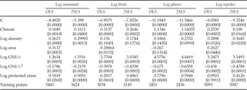
In order to test the relation between income and the threat to biodiversity without relying on forest area as a proxy, Perrings and Halkos (Reference Perrings and Halkos2010) model the relation between GDP per capita and threats to each of four taxonomic groups – mammals, birds, plants, and reptiles – while controlling for the effects of climate, population density, land area, and protected area status. Using the number of species in each taxonomic group under threat (according to the 2004 IUCN Red List) as the response variable, they model the relation between the level of threat and Gross National Income per capita in a sample of 73 countries. In the absence of a usable time-series for the response variable, this implies a cross-sectional analysis. Controls include climate, total and protected land area, and (human) population density. Climate is measured by a dummy variable indicating whether a country fell wholly or partly in the Koppen–Geiger equatorial climates and controls for the effect of species richness. Land area controls for the effect of country size, and the percentage of land area under protection controls for the availability of refugia. Population stress was proxied by population density.
They found that once climate, land area, population density (pressure), and the land area under protection are controlled for, the relation between income and species under threat turns out to be strongly quadratic for all terrestrial species. The turning points are different for different taxonomic groups but all models provide a good fit to the data, and satisfy a range of diagnostic tests (see table 1). Since there is a potential simultaneity problem involved in the control for protected areas – that the size of protected areas may be a reflection of the number of species under threat – they modeled protected areas both as an independent variable (using ordinary least squares), and as an endogenous variable, instrumented on land area and the number of species under threat in other taxonomic groups (using two stage least squares). The results of the two models are consistent. Nor did a quantile regression show the effect to be sensitive to the level of risk.
Factors associated with threats to biodiversity (OLS and 2SLS model results)

P values in parentheses.
Source: Perrings and Halkos (Reference Perrings and Halkos2010).
The implication is that in the poorest countries, income growth is strongly correlated with increasing levels of threat to biodiversity. The result reflects the fact that the poorest countries are also quite strongly agrarian. In such countries, income growth depends both on the extensive growth of agriculture – the expansion of agricultural lands into more ‘marginal’ areas that are otherwise habitat for wild species, and on agricultural intensification – the progressive simplification of the agroecosystem as pests, predators, and competitors are ‘weeded out’ of the system. While there is the potential to design agroecosystems in ways that reduce the biodiversity/agricultural output tradeoff (Jackson et al., Reference Jackson, Pascual, Brussaard, De Ruiter and Bawa2007), the empirical evidence is that in low-income countries increasing agricultural output has the highest priority.
In terms of the models of biodiversity discussed earlier (Brock and Xepapadeas, Reference Brock, Xepapadeas, Kristrom, Dasgupta and Lofgren2002; Brock et al., Reference Brock, Kinzig and Perrings2010), these two trends imply the homogenization of the system, a reduction in niche differentiation, and hence a reduction in species richness. The existence of a turning point indicates that at some level of per capita incomes and at some level of biodiversity threat the marginal value of land committed to biodiversity conservation dominates the marginal value of land committed to agriculture, inducing a change in the allocation of land resources to allow greater niche differentiation. One dimension of this is the establishment of reserve areas characterized by high levels of heterogeneity (whether in a few large heterogeneous areas or a number of smaller areas distributed across an ecological gradient). A second dimension is the establishment of separate niches within existing agroecosystems (through, for example, the promotion of riparian corridors).
The evidence on the biosecurity dimensions of the problem is similarly different in developed and developing countries. If we take trade-related pest and pathogen risks, the fact that developed countries have higher levels of imports means that they are more exposed to the risk of introductions. At the same time, the likelihood that introduced species will establish and spread depends on the public health, SPS efforts undertaken by a country. Since public health, SPS effort will increase up to the point at which the marginal benefit (damage avoided) is equal to the marginal cost of that effort, we would expect greater levels of effort in countries where the value at risk is higher. So while developed countries are more exposed, they also invest more in public health, SPS measures.
The result of this is that developing countries are generally more exposed to damaging pests and pathogens. For example, Pimentel's (Pimentel et al., Reference Pimentel, Mcnair, Janecka, Wightman, Simmonds, O'Connell, Wong, Russel, Zern, Aquino and Tsomondo2001) estimates of the damage costs associated with introduced plant pests in a selection of developed and less developed countries in the 1990s suggested that invasive species caused estimated damage costs equal to 53% of agricultural GDP in the USA, 31% in the UK and 48% in Australia. By contrast damage costs in South Africa, India, and Brazil were estimated to be, respectively, 96%, 78%, and 112% of agricultural GDP.
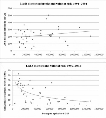
The different exposure is particularly easy to see in the case of animal diseases, as is the difference in response. Until recently, the World Organization for Animal Health (OIE) categorized the species reported to it according to both their rate of spread and potential damage. One category, List A species, comprised transmissible diseases with the potential for very serious and rapid spread, significant damage costs and potentially major negative effects on public health. A second category, List B species, comprised transmissible diseases with slightly less significant damage costs. Analysis of the relation between the number of outbreaks within each category of disease and the value at risk indicates that whereas outbreaks of most diseases (i.e., List B diseases) increased with the volume of imports, outbreaks of List A diseases decreased (see figure 1). The implication is that, for these classes of pests, countries in which the value at risk is high implement sufficiently stringent sanitary measures to offset the introduction risk associated with high levels of imports.
The relation between outbreaks of notifiable animal diseases and value at risk, 1996–2004
Source: Data sourced from the OIE and COMTRADE databases.

5. Discussion
The research and policy agendas on biodiversity have evolved together. As the problems posed by emergent zoonotic diseases and other invasive species have become more transparent, so has research on the problems expanded. But even though it is becoming increasingly clear that the three dimensions of the problem are present in most examples of biodiversity change, they are seldom treated as components of a common problem. Nor is science better at connecting the pieces of the puzzle than policy. Indeed, just as the institutional divisions between production, conservation, and biosecurity have made cooperation across the multilateral agreements set up to address these three dimensions of the problem problematic, so divisions between the disciplines associated with each dimension have complicated the development of an integrated biodiversity science. Institutionally, the conservation and production oriented multilateral environmental agreements reflect the deep seated mutual suspicion of the national agencies charged with promoting each, while the agreements concerned with human, animal, and plant health are isolated from both. But the academic disciplines involved in each are generally no less reluctant to bridge the gap. Collaboration across conservation biology, ecology, agronomy, forestry, aquaculture, public health, epidemiology, entomology, veterinary science, and the key social sciences remains weak. So while economists have sought to model both the cross-sectoral externalities and the tradeoffs involved in addressing the three dimensions of the biodiversity problem, the models still rest on weak foundations.
A second aspect of the scientific problem that remains a challenge is the question of scale. From a policy perspective, the central problem in the international governance of biodiversity is the fact that it affects the delivery of ecosystem services at many scales. A change in the number and abundance of species in any one location may have consequences for a bundle of ecosystem services/disservices, each of which is associated with benefits or costs realized at a different spatial and temporal scale. Some of these benefits are clearly global public goods – such as the climatic effects of carbon sequestration, the control of zoonotic diseases with potential to become pandemic, or the conservation of the genetic information in land races or wild relatives. Others are public goods at regional, national, or local scales. The role of biodiversity in protecting watersheds, for example, offers benefits at multiple scales – from the regional scale in the case of major river basins all the way down to local catchments. On the other hand, the functional diversity of pollinators almost always delivers benefits at a local scale. More importantly, the value of biodiversity in assuring the supply of particular services over a range of environmental conditions is highly sensitive to the time horizon chosen. The value of species that are functionally redundant in any given set of conditions depends on the likelihood that conditions will occur in which they are not redundant, and this increases with the time over which environmental conditions are allowed to vary. Perrings and Gadgil (Reference Perrings, Gadgil, Kaul, Conceicao, Le Goulven and Mendoza2003) described biodiversity conservation as a ‘layered’ public good since the same set of species may be implicated in the delivery not just of an array of services over a range of spatial and temporal scales, but also a number of different types of public good.
The development of spatially explicit models of ecosystem services associated with different types of land use and land cover is a significant recent development (Nelson et al., Reference Nelson, Polasky, Lewis, Plantinga, Lonsdorf, White, Bael and Lawler2008; Polasky et al., Reference Polasky, Nelson, Camm, Csuti, Fackler, Lonsdorf, Montgomery, White, Arthur, Garber-Yonts, Haight, Kagan, Starfield and Tobalske2008; Nelson et al., Reference Nelson, Mendoza, Regetz, Polasky, Tallis, Cameron, Chan, Daily, Goldstein, Kareiva, Lonsdorf, Naidoo, Ricketts and Shaw2009). However, while these models have made it possible to evaluate tradeoffs between some services – and especially tradeoffs between the biodiversity conservation and carbon sequestration – they have not begun to address tradeoffs in functional diversity at different temporal scales. Nor do they address the distribution of many of the most important offsite costs and benefits of on-site biodiversity change. These remain challenges for the future.
The development of instruments designed to provide landholders with the ‘right’ incentives depends on progress in both dimensions of the problem. It is not sufficient to have good physical measures of changes in ecosystem services. It is also necessary to have good estimates of the social opportunity cost – the value – of these changes. The ongoing assessment of the economics of ecosystem services and biodiversity (TEEB) has approached this by averaging across valuation studies of specific services. TEEB shows that, on this basis, the value of tropical forests is dominated by regulatory functions: specifically regulation of climate ($1965/ha/year), water flows ($1360/ha/year), and soil erosion ($694/ha/year). The mean value of other services combined – timber and nontimber forest products, food, water, genetic information, pharmaceuticals ($1313/ha/year) is less than the value of water flow regulation alone (TEEB, Reference TEEB2009). While this says nothing about the marginal value of specific services in particular locations, it does suggest that the efforts to use incentives to enhance the flow of ecosystem services might be best directed at the regulating services. In fact, the development of local markets in ecosystem services using systems of Payments for Ecosystem Services has focused on three things: carbon sequestration as a means of regulating the climate, watershed protection as a means of regulating water quality and quantity, and biodiversity conservation. The best known examples are the Reduced Emissions from Deforestation and Forest Degradation (REDD) scheme, which is intended to generate payments for carbon sequestration, and the REDD plus scheme which adds conservation as an incidental benefit (TEEB Reference TEEB2009; O'Connor, Reference O'Connor2008). PES schemes have also been developed that offer financial incentives for landholders to provide more localized external, nonmarket ecosystem services (Engel et al., Reference Engel, Pagiola and Wunder2008).
So while the economics of biodiversity has developed in ways that have strengthened both the analysis and policy relevance of research, there is still much to do. The many and varied linkages between biodiversity change and human well being in developing countries are not yet well understood. Nor are the tradeoffs between ecosystem services that provide public benefits at widely varying spatial and temporal scales. The addition of spatially explicit models of the physical tradeoffs between ecosystem services in particular locations is a major step forward, but unless accompanied by models of the social opportunity cost to those with an interest in that location has limited value for decision support. Given the agreement to establish an Intergovernmental Science-Policy Platform on Biodiversity and Ecosystem Services, we may expect to see a significant increase in the demand for economic analysis of biodiversity change. Developments in the field over the life of EDE have improved its capacity to meet that demand, but we need to build that capacity much further.