
Introduction
Kinetic Monte Carlo (KMC) is often the method of choice while studying the long-time dynamical evolution of molecular- and meso-scale materials and biomolecular systems.[Reference Chatterjee and Vlachos1–Reference Gilmer, Huang, de la Rubia, Dalla Torre and Baumann5] To generate dynamical trajectories of the system, a KMC model requires a catalog of metastable states, i.e., long-lived configurations of the system, and the kinetic pathways that specify how fast the system can interconvert between the states. In KMC, pathways are defined in terms of the starting and end states and their associated rate constants. The continuous time trajectories generated using a KMC model are available as “discrete” state-to-state transitions. Achieving dimensionality reduction from the large number of atomic degrees of freedom to a significantly smaller “network” of states constitutes a major advantage of the KMC method. However, the same property also introduces a challenge since the catalog of states and pathways is generally not known at the outset for most complex materials and biomolecules.[Reference Henkelman and Jonsson6] For instance, configurations visited during the unfolding of a protein from its folded state might be unknown but these states are required as an input in the KMC model to accurately describe the dynamical unfolding process.[Reference Chatterjee and Bhattacharya7, Reference Bhoutekar, Ghosh, Bhattacharya and Chatterjee8]
To address this issue, KMC models can be constructed using molecular dynamics (MD).[Reference Voter, Sickafus, Kotomin and Uberuaga2, Reference Gilmer, Huang, de la Rubia, Dalla Torre and Baumann5, Reference Chatterjee9] In MD, one solves the Newton's equations of motion to generate dynamical trajectories.[Reference Frenkel and Smit10] The input provided to an MD calculation includes the initial atomic positions and velocities, the MD time-step (typically in femtoseconds) and an interatomic potential or a force field for the system. MD is computationally more expensive than KMC. One can have best of both worlds by learning about the discrete states and kinetic pathways of the system by post-processing several independent MD trajectories to generate a concise KMC model.[Reference Pande, Beauchamp and Bowman11, Reference Prinz, Wu, Sarich, Keller, Senne, Held, Chodera, Schütte and Noé12] States and pathways sampled in the MD trajectory are incorporated into the KMC model. Alternatively, we can direct our efforts toward parts of the configurational space that we think are important for the construction of the KMC model. In such a case, transitions are sought only from chosen states using MD to prepare a KMC model “on-the-fly”. In either case, even when terabytes of MD data is available, the resulting KMC model will be only as good as the MD data used to construct it. A related issue is the underlying network complexity, namely, states that are relevant to the dynamics can be extremely large in number and hard to guess,[Reference Haldar and Chatterjee13–Reference Chill and Henkelman15] which precludes the construction of “complete” KMC catalogs.[Reference Bhoutekar, Ghosh, Bhattacharya and Chatterjee8, Reference Bhute and Chatterjee16, Reference Bhute and Chatterjee17]
It becomes important to ascertain the uncertainty in the KMC model before the model is used to generate long-time dynamical trajectories and gain new physical insights. The KMC model has an uncertainty associated with it because of the states and pathways missing in the MD data. Uncertainty quantification helps us assess how important the missing information could be to the true dynamical evolution of the system.[Reference Chatterjee and Bhattacharya7, Reference Chill and Henkelman15–Reference Bhute and Chatterjee17] We answer the following questions:
• How does one determine uncertainty in a KMC model from the MD data used to construct the model?
• If there were provision for additional MD, is there an optimal way to generate high-quality MD data which lower the uncertainty?
Since the true dynamics is not known to us, the model uncertainty is based on probability theory. The strategy used revolves around two key points. First, pathways that are likely to be selected in the dynamics should be present in the KMC model. As long as the missing pathways continue to be selected with an extremely low probability, they are deemed less relevant to the dynamics and can be missing from the model without affecting the KMC accuracy. “Excellent sampling” of a state in question can guarantee that (at least up to a certain timescale) most of the relevant pathways from the state would be present in the catalog. Issues related to missing pathways also arise in some accelerated MD techniques.[Reference Sorenson and Voter18] Second, optimal usage of the computational resources requires that states likely to be visited in the dynamics should be studied in detail using MD. As long as other states are visited with a lower probability, they can be ignored while sampling the configurational space. A KMC model that appears to be reasonably accurate at short timescales can become grossly inaccurate at longer timescales where the missing states and pathways matter to the dynamics. Thus, uncertainty in the KMC model is a timescale-dependent property, which is captured by a quantity we term as validity time of the KMC model. A KMC model remains accurate (with a confidence level) till its validity time. A detailed discussion on uncertainty in the KMC model constructed using MD can be found in Ref. Reference Bhoutekar, Ghosh, Bhattacharya and Chatterjee8. Biomolecular simulations often employ Markov State Models (MSMs) that are closely related to the KMC models. MSMs are constructed using post-processing of MD trajectories.[Reference Schwantes, McGibbon and Pande3] Therefore, the ideas presented here are useful to the practitioners of both KMC and MSM approaches.
Questions related to the completeness of the KMC model created using dynamical approaches[Reference Bhoutekar, Ghosh, Bhattacharya and Chatterjee8, Reference Bhute and Chatterjee16, Reference Bhute and Chatterjee17] require slightly different terminology from non-dynamical approaches.[Reference Boulougouris and Frenkel19–Reference Xu and Henkelman21] Since the KMC model uncertainty is a timescale-dependent property, dynamical approaches are better suited toward uncertainty quantification. In this article, we provide a review on a computational procedure that can (i) construct KMC models on-the-fly using MD, (ii) measure the uncertainty in the current KMC model, and (iii) optimally target uncertain regions of configuration space for further network construction. “Two extreme KMC model construction examples” section provides two examples to motivate the need for on-the-fly KMC model construction using MD. A step-by-step description of the construction procedure is provided. The basis for uncertainty quantification of the KMC model is discussed. It is important to recognize that accessing long timescales with MD can be prohibitively expensive. Typically, standard MD is restricted to the μs timescales, whereas KMC can easily access ms timescales and beyond with significantly smaller computational resources. Two novel enhanced sampling strategies are described next, which can be used to seek pathways rarely selected with standard MD. These methods offer significant advantages over regular MD and help lower the uncertainty in the KMC model in a very efficient manner.
Two extreme KMC model construction examples
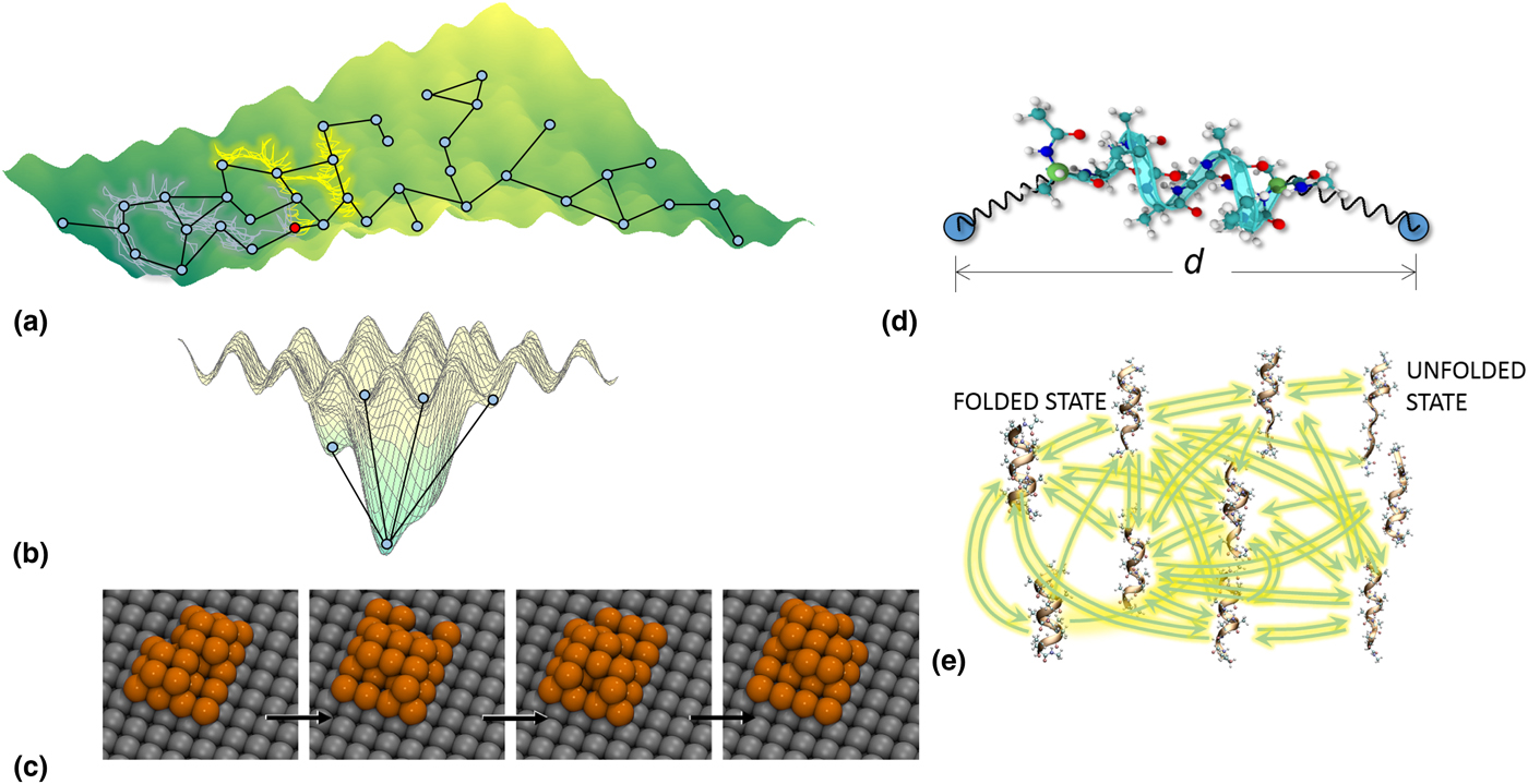
A KMC model can be described in terms of a directed network with the nodes representing the states and edges/connections representing the pathways [Figs. 1(a) and 1(b)]. The potential energy surface (PES) is a useful concept to visualize the dynamics.[Reference Wales22] The landscape contains several minima. A state of the system can contain one or more minima, such that it is a long-lived configuration. The number of connections between the states, i.e., the network complexity, depends on the underlying PES. It is essential to distinguish between the two extreme forms of landscapes. The first one involves a “diffuse” energy landscape characterized by a large number of states [Fig. 1(a)]. The probability of the system visiting these states is low as the system can select one of many possible pathways during the evolution. The other extreme involves a funnel-shaped landscape, which generally would contain a small number of states (<1000) and the system will remain trapped in these states [Fig. 1(b)]. Two examples of these landscapes are provided next to highlight similarities and differences in the KMC model development and uncertainty quantification. In general, landscapes can contain features corresponding to both Figs. 1(a) and 1(b).
Schematic representation showing two extreme examples of potential energy surfaces: (a) diffuse and (b) funnel-shaped landscape. Circles denote long-lived metastable states of the system. Straight lines denote kinetic pathways between states. Random gray and yellow lines in panel a denote MD trajectories initiated from the red-colored state. (c) Evolution of an Ag nanocluster on Ag(100) at 300 K. (d) A deca-alanine molecule with force applied at its two ends. The anchor separation is kept at d. (e) Network model constructed for stretched deca-alanine molecule. Adapted with permission from Ref. Reference Ghosh, Chatterjee and Bhattacharya27, American Chemical Society, 2017.

Figure 1(c) shows structural rearrangements observed in 26-atom Ag cluster on Ag(001) surface studied using KMC. The Ag cluster evolves on a diffuse landscape from an initially less-compact structure and becomes more compact as time progresses. The Ag cluster can evolve from its initial state in many different ways but the pathways are not known initially. A state is described in terms of its all atom coordinates. Kinetic pathways from states were sought using MD calculations. Two hundred fifty-five MD calculations were performed in the current state at 300 K. Each MD calculation was independent by virtue of the random seeds used to initialize the trajectories in the state. An MD calculation was stopped once a transition from the state was detected. Thus, the 255 MD calculations enabled construction of a catalog of kinetic pathways from the current state, and new states are now known to us. Additional MD calculations performed in the state could lead to further discovery of connected states. The completeness of the catalog is a function of the total MD simulation time t S elapsed in a state S.
An extensive search over the configurational space using 255 processors over 18 days yielded 9964 states and 16,475 kinetic pathways. The model is more accurate than standard lattice KMC models used in the literature. Standard models incorrectly assume that the cluster evolves only via hopping and exchange mechanisms. MD calculations clearly demonstrate that several important concerted atom moves, which are not accounted in the standard models, play an important role in the dynamics (see Supplementary Material). As a consequence, the timescales of evolution from the lattice-based KMC models would significantly differ from an MD-based KMC model. In addition, many off-lattice states need to be included in the KMC model (see Supplementary Material). Determining all possible states and mapping the connectivity between the states is an impossible task. Use of pattern-recognition schemes that reuse previously discovered kinetic pathways for similar looking local atomic environments can aid in the construction of the KMC model.[Reference Konwar, Bhute and Chatterjee23] In addition, rates for certain types of mechanisms found that using MD calculations can be extended to new atomic environments, which remain unexplored using cluster expansion[Reference Verma, Rehman and Chatterjee24–Reference Kulkarni and Chatterjee26] and neural-network techniques.
The second example involves stretching of a deca-alanine molecule by maintaining the distance d between two anchor points (blue circles) shown in Fig. 1(d). The ends of a molecule are attached to the anchor points mimicking a force spectroscopy setup. The initial state of system corresponding to a folded structure is specified [Fig. 1(e)]. Guessing the states and pathways is impractical. States of deca-alanine and their connectivity are discovered using 300 independent MD calculations at a time for a state in question. After 3 days of computational time, 810 states and more than 1000 kinetic pathways are known. The state recognition scheme involved comparing the backbone atoms after aligning the molecule using the Kabsch algorithm.[Reference Bhoutekar, Ghosh, Bhattacharya and Chatterjee8] The PES for the stretched deca-alanine is funnel-shaped. As a result, the system remains trapped mostly in the ten states in Fig. 1(e) for 95% of the time when d <24 Å. The KMC model in the form of a network is shown in Fig. 1(e). However, this behavior changes for higher extensions and knowledge of frequently visited states and their conformational properties becomes essential toward the calculation of the average forces experienced by the anchors. It is always possible that some states and pathways that are accessed at much longer MD timescales remain to be discovered. One would like to calculate the uncertainty in the two models despite differences in the network topology.
On-the-fly construction of a KMC model and its uncertainty
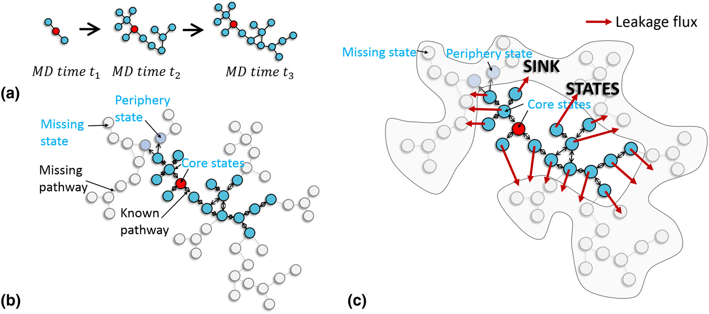
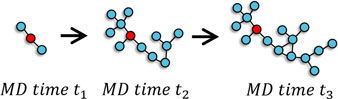
A step-by-step procedure to generate a KMC model using MD is described next. Consider the initial state S shown in red in Fig. 2(a). An MD calculation is performed in state S [red circle in Fig. 2(a)] in the canonical ensemble till a transition from the state is detected. The new state of the system and the waiting time are noted. As mentioned earlier, kinetic pathways are defined only in terms of their initial and final states. Additional waiting times are collected by seeding independent MD trajectories from S. The advantage of constraining the system to state S is that it prevents the system from performing a random walk on the energy landscape and a large number of transitions from S can be sought. We term this procedure as the state-constrained MD method. Next, the rate constant k p for a pathway p is estimated using a statistical technique. For instance, the estimate using the maximum-likelihood analysis is given by
 $$k_p = n_p/\tau _{S,p},$$
where n p is the number of transitions involving p and τ S,p is the time elapsed in state S for the n p transitions. Independent MD trajectories can be generated in parallel when multiple processors are available. The total MD time invested into the construction of the model [with two pathways from state S as shown in Fig. 2(a)] is t 1.
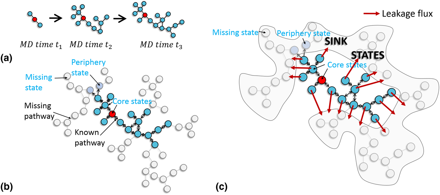
(a) Growing kinetic network model as a function of the duration of the molecular dynamics (MD) calculations. (b) Types of states in the network model: core (blue and red circles), periphery (gray-filled circles), and missing states (white circles). (c) Schematic representation illustrating the concept of leakage flux from the core states.
The kinetic information content, e.g., states visited, waiting times, in a single trajectory is limited and varies from one trajectory to another. It becomes important to compile the behavior of a large collection of trajectories and to assess the missing kinetic information in terms of the ensemble. The probability of residing in state S at time t is given by the state occupation π S. The dynamics of first-order processes is described by the master equation:
 $$\displaystyle{d \over {dt}}\pi _S(t) = \mathop \sum \limits_{S{\rm ^{\prime}} \ne S} k_{S{\rm ^{\prime}} \to S}\pi _{S^{\prime}} - \mathop \sum \limits_{S{\rm ^{\prime}} \ne S} k_{S \to S{\rm ^{\prime}}}\pi _S.$$
The rate of change in π S is given by the probability flux into S minus the probability flux out of state S. Writing Eq. (2) requires as an input the catalog of states and pathways discovered in our MD trajectories. Therefore, Eq. (2) captures our current understanding of the dynamics. Since in our present KMC model (MD time t 1) only pathways from state S have been sampled [Fig. 2(a)], the rates constants  $k_{{S}^{\prime} \to S} = 0,\; \,\forall \; {S}^{\prime} \ne S$. Equation (2) reduces to
 $d[\pi _S(t)]/dt = - \sum\nolimits_{{S}^{\prime} \ne S} {k_{S \to {S}^{\prime}}\pi _S} $. We term state S as a core state as the state has been sampled and one or more pathways from the state are known. States S ′ ≠ S are termed as the periphery states of the model since they have not been adequately sampled and none of the pathways from S ′ are known. States that have not been visited so far in the MD calculations are called missing states. For the periphery states,
 $d[\pi _{S^{\prime}}(t)]/dt = k_{S \to S{\rm ^{\prime}}}\pi _S$ highlights that the core states are source and periphery states are sink states. It is shown later that missing states are also sink states. The periphery states can be converted one-by-one into core states by performing MD in these states. For instance, MD calculations performed in a periphery state S ′ may reveal a pathway from S ′ to S ′′, which was not present in the KMC model earlier. In the process, the network model grows and many new periphery states can emerge. Figure 2(a) shows a schematic of the growing network model as a function of the MD time. In Fig. 2(a), the MD time invested t 1, t 2, and t 3 are well separated so that significant changes in the model topology is observed. Blue circles in Fig. 2(a) are states discovered using MD. We shall later discuss a systematic strategy to determine which periphery or core states need to be optimally explored.
Defining the KMC model as one consisting only of the core (C) states [see red and blue states in Fig. 2(b)] ensures that the system reaches a steady state. Thus, the KMC model is given by
 $$ \displaystyle{d \over {dt}}{\tilde \pi}_S(t) = \mathop \sum \limits_{\matrix{{{S}^{\prime} \in C} \cr {{S}^{\prime} \ne S} \cr}} (k_{{S}^{\prime} \to S}{\tilde \pi}_{{S}^{\prime}} - k_{S \to {S}^{\prime}}{\tilde \pi}_{\rm S}),\; \;S \in C.$$
The tilde in Eq. (3) emphasizes that the system of equations is different from the one in Eq. (2). White circles in Fig. 2(b) denote the states that are missing (M) from the model. A more complete model would have included some of the missing states. Since  $k_{{S}^{\prime} \to S},\;{S}^{\prime} \in M$ is not known, we assume these rates to be zero. Estimates for
 $k_{S \to {S}^{\prime}},\;\; {S}^{\prime} \in M$ are obtained later. The missing and periphery states are lumped together into the sink states, which allow us to write the full network model
 $$\eqalign{\displaystyle{d \over {dt}}{\hat \pi}_S(t) & = \mathop \sum \limits_{\matrix{{{S}^{\prime} \in C} \cr {{S}^{\prime} \ne S} \cr}} (k_{{S}^{\prime} \to S}{\hat \pi}_{{S}^{\prime}} - k_{S \to {S}^{\prime}}{\hat \pi}_S) \cr & - \mathop \sum \limits_{{S}^{\prime} \in P \cup M} k_{S \to {S}^{\prime}}{\hat \pi}_S,\;\; {S \in C}.}$$
In comparison with Eq. (3), Eq. (4) additionally contains the leakage flux to the missing and periphery states. The caret indicates that the solution to Eq. (4) can be different to the one from Eq. (3). A similar approach has been used in Ref. Reference Boulougouris and Theodorou20 without accounting for the missing states.
Figure 2(c) explains the full network model using a schematic representation. Probability from core states (blue or red circles) can leak (red arrows) into the periphery and missing states (shown in gray and gray-blue circles, respectively, within the gray-shaded region). The system cannot return to the core states as pathways from the sink to core states are unknown. The KMC model behaves identically to the full network model as long as the leakage to sink states remains small. An upper bound for the probability flux from a core state S to the sink states is obtained. This bound is termed as the leakage flux F S [see Fig. 2(c)]. The leakage flux is given by
 $$F_S = \hat \pi _S\left( {\mathop \sum \limits_{{S}^{\prime} \in P} k_{S \to {S}^{\prime}} + \mathop \sum \limits_{{S}^{\prime} \in M} k_{S \to {S}^{\prime}}} \right).$$
The leakage flux is small as long as  $\hat \pi _S$ or
 $\sum\nolimits_{{S}^{\prime} \in P} {k_{S \to {S}^{\prime}}} + \sum\nolimits_{{S}^{\prime} \in M} {k_{S \to {S}^{\prime}}} $ or both are small. The leakage rate to the periphery states
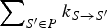 $\sum\nolimits_{{S}^{\prime} \in P} {k_{S \to {S}^{\prime}}} $ in Eq. (5) is already known from MD calculations. The leakage rate to missing states is obtained from the available MD data. Estimates for the missing rates of the form
 $$\mathop \sum \limits_{{S}^{\prime} \in M} k_{S \to {S}^{\prime}} = \displaystyle{{\ln (1/\delta )} \over {t_S}} + k_b(N_b - n_b).$$
were obtained in Ref. Reference Bhute and Chatterjee16. When the number of pathways from a state is small, the missing rate is bounded by ln (1/δ)/t S. Here t S is the MD time spent in the state S and 1 − δ is the confidence, such that 0 < δ <1. Non-dynamical sampling techniques[Reference Boulougouris and Frenkel19–Reference Xu and Henkelman21] cannot provide estimates for the missing rate from a state since t S is not available. Low values of δ (typically δ < 1) are used. Additional corrections given by the second term in Eq. (6) are needed when a large number of pathways, N b in number, from S possess similar values of rate constants. These pathways occur at the current timescales t S. Suppose only N b of the N b pathways from S have been sampled. Letting k b denote the average rate for the frequency band b, the goal is to determine N b. The number of transitions involving the pathways p 1, p 2, …,  $p_{N_b}$ is distributed according to the multinomial distribution
 $$p(n_{\,p1},n_{\,p2}, \ldots, n_{\,pN_b}) = \displaystyle{{n_S!} \over {\mathop \prod \nolimits_{\,p = 1,2, \ldots, N_b} (n_p!)}}\mathop \prod \limits_{\,p = 1,2, \ldots, N_b} \left( {\displaystyle{1 \over {N_b}}} \right)^{n_p}\;. $$
The correction, which involves estimating N b from the waiting times sampled for N b pathways, can be ignored when N b <10.
Three questions can be addressed as this point:
I. How to quantify the error in Eq. (3)––the KMC model.
II. Find how long Eq. (3) can faithfully predict the dynamics by estimating the uncertainty in the model.
III. How to perform the MD sampling to reduce the uncertainty.
The difference between the two models  $\hat \pi _S(t) - \tilde \pi _S(t)$ remains small as long as the total leakage flux from the core states is negligible. The timescales where the two models begin to diverge determines the validity time for the KMC model. The validity time allows systematic comparison of the two models of the same system constructed with different amounts of MD time in each state, while accounting for known kinetic rates, topology, and relaxation times of the network as well as pathways and states missing from the model. The missing and periphery states may become important to the dynamics beyond the validity time of the model. The KMC model can be regarded as complete with confidence (1 − δ) till the validity time. We illustrate some of these points next.
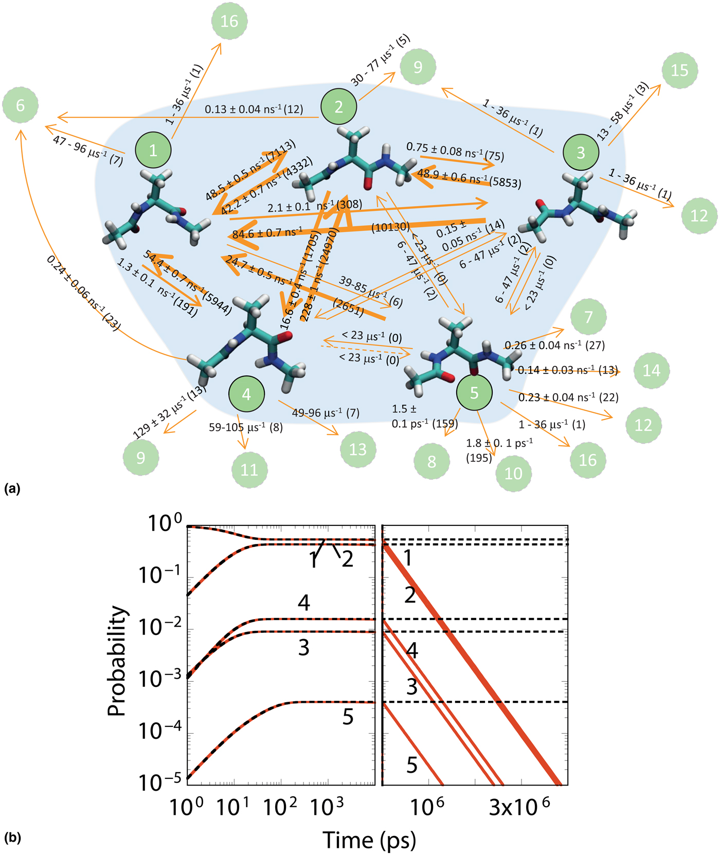
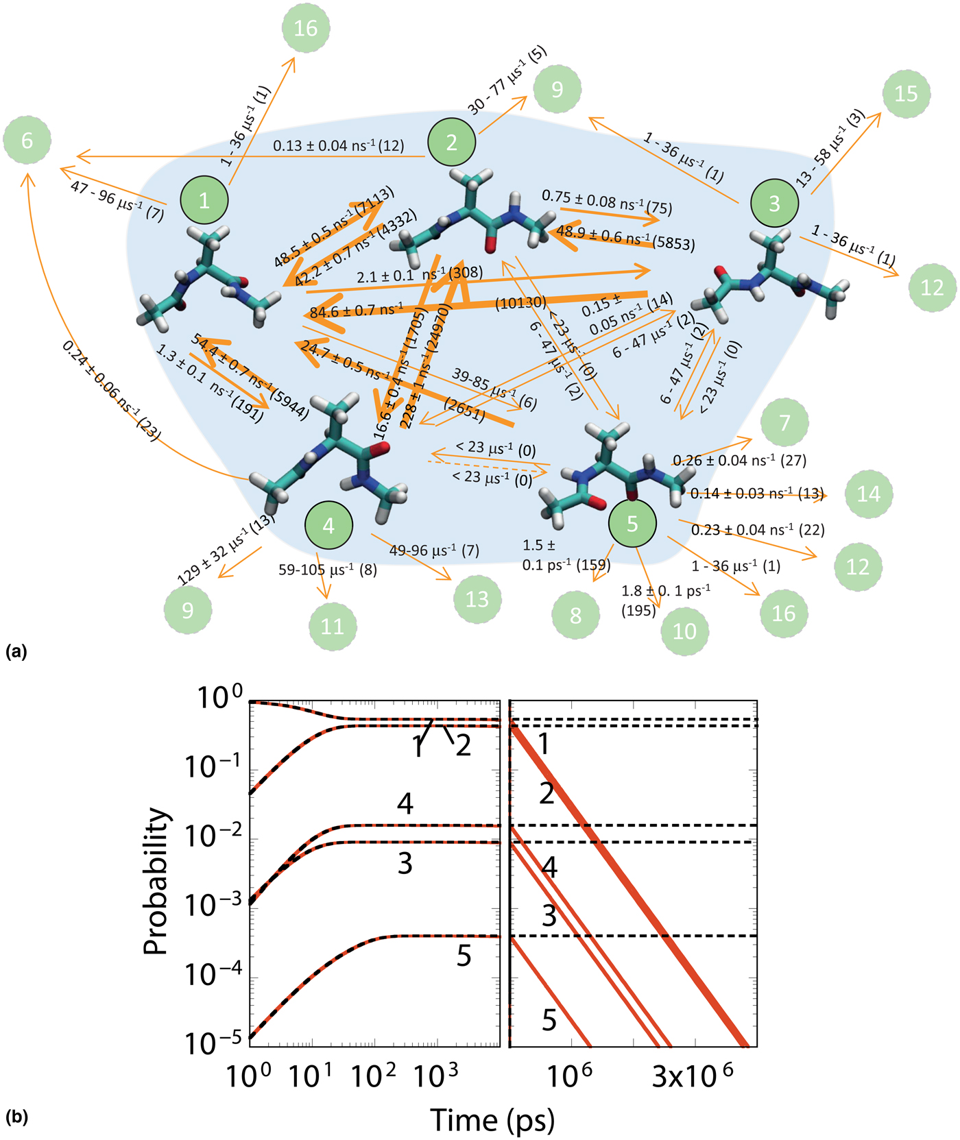
Figure 3(a) shows an example with a single alanine dipeptide molecule in solvent. Initially only state 1 is known to us. State-constrained simulations were performed in state 1, which resulted in the discovery of states 2–4 with relatively few MD calculations. The transition to state 5 is rare and therefore it took a longer time to discover the pathway from state 1 to 5. Rates from state 1 calculated using Eq. (1) for the different pathways are shown in the figure next to the arrows. The number in parentheses next to the rate constant gives the number of MD calculations used to estimate the rate. Similarly, we performed several thousand MD calculations in states 2–5 to learn about the pathways on-the-fly as the trajectories are generated in parallel. Note that pathway from state 3 to 5 was not sampled but missing rate from state 3 can be estimated using Eq. (6). The total MD time invested in building the five core state (states 1–5) KMC model exceeded 0.3μs. Eleven periphery states (states 6–16) are found. These states are shown in the dotted circles in Fig. 3(a). Solving the KMC model [i.e., Eq. (3) with only core states] shows that the system largely resides in states 1 and 2. The full model [Eq. (4)] contains the five core and sink states. Since the flux from states 1–5 to states 6–16 are small, MD calculations were not performed in states 6–16. This aspect can be easily checked by comparing the time-dependent occupations from the KMC model [black lines in Fig. 3(b)] and the full model [red lines in Fig. 3(b)]. The models agree till about 0.1μs beyond which the leakage to the periphery and missing states becomes significant for us to lose confidence in the KMC model. The validity time for the KMC model is 0.1μs. Missing states and pathways in the KMC model can become important to the dynamics after the time simulated with the KMC model exceeds its validity time.
(a) Kinetic network model for solvated alanine dipeptide containing 16 states. States 1–5 form the core states while 6–16 are periphery states. (b) Calculation of the validity time for the kinetic network model. Adapted with permission from Ref. Reference Bhoutekar, Ghosh, Bhattacharya and Chatterjee8, AIP Publishing, 2017.
Post-processing of MD trajectories can be used to create a fresh KMC model or update a pre-existing KMC model. The validity time for the resulting model is obtained as follows:
Step 1: Identify the states and pathways of the material/biomolecular system from the collection of MD trajectories. Obtain rate constants for pathways using a statistical approach, e.g., using Eq. (1), provided the number of transitions for the pathway n p is large enough for us to calculate the rate with a high confidence.
Step 2: Determine the core and periphery states in the updated KMC model.
Step 3: Use Eq. (6) to calculate the missing rate from each core state (in case the core state has been updated).
Step 4: Construct the KMC [Eq. (3)] and full network model [Eq. (4)].
Step 5: Solve the system of equations in Eqs. (3) and (4) to obtain the dynamical evolution  $\tilde \pi _S(t)$ and
 $\hat \pi _S(t)$, respectively.
Step 6: The validity time is determined as the time where  $\tilde \pi _S(t)$ and
 $\hat \pi _S(t)$ begin diverge.
An automated procedure called the programmed state-constrained MD to efficiently build the KMC model was reported in Ref. Reference Bhoutekar, Ghosh, Bhattacharya and Chatterjee8. The procedure involves systematically finding the largest leakage rates and performing additional MD to plug the probability leakage from the core states. When the leakage to a specific periphery state S ′ is the largest source of leakage in Eq. (4), MD calculations are performed in the periphery state S ′ so that pathways from S ′ can be discovered and S ′ converted to a core state. On the other hand, when the largest leakage results from a core state S to missing states performing MD in S is recommended in order to lower the missing flux. The programmed state-constrained MD enables automatic construction of the KMC model in the most efficient manner. The main steps involved are a continuation of steps 1–6 described earlier:
Step 7: Calculate the leakage flux from each core states using Eq. (5) at the point where  $\tilde \pi _S(t)$ and
 $\hat \pi _S(t)$ begin diverge, i.e., at the validity time.
Step 8: Identify sources of large leakage. When a significant leakage occurs from a core state S to a periphery state S ′ additional MD should be performed in the periphery state S ′. On the other hand when the missing flux from a core state S is large, additional MD is required in the core state S.
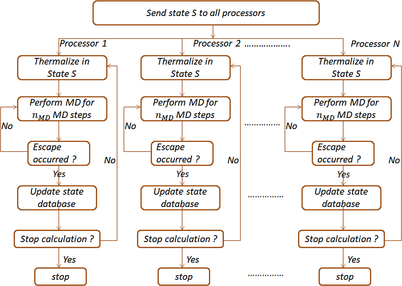
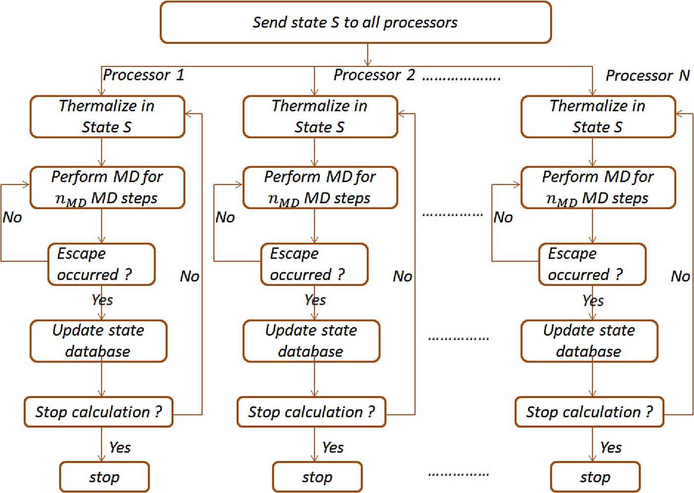
Step 9: Perform additional MD in states that associated with large leakage. For instance, significant improvement can be made to the network model by generating 100 or more short MD trajectories. These could be state-constrained MD trajectories ending with a transition. Figure 4 shows the flow chart for the state-constrained MD calculations.
Flowchart for the state-constrained MD calculation. Depending on the material/biomolecular system typically n MD is chosen such that the corresponding time is smaller than the average waiting time for a transition from state S.
Step 10: Go to step 1 and continue as long as a target validity time is achieved or until more computer time can be afforded.
Accelerated construction of KMC models
When the system is equilibrated in N trapping core states corresponding to deep basins in the funnel-shaped energy landscape, the total leakage rate for the network is 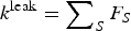 $k^{{\rm leak}} = \sum\nolimits_S {F_S} $. It can be shown that
 $k^{{\rm leak}} = N\tau _{{\rm MD}}^{ - 1} \ln \, (1/\delta )$, where τ MD is the total MD time. The validity time is approximately given by (k leak)−1, i.e., validity time scales as τ MD. Accelerated techniques can help increase the validity time and reduce the KMC model uncertainty by revealing missing pathways from core and periphery states. A number of (dynamical) enhanced sampling techniques[Reference Voter, Montalenti and Germann28–Reference Laio and Parrinello31] are available that can readily access orders-of-magnitude longer times t S or τ MD than possible with regular MD. Recent examples of exploiting dynamical-enhanced sampling techniques include Ref. Reference Chatterjee and Bhattacharya7, Reference Chill and Henkelman15, Reference Chatterjee and Bhattacharya32 and Reference Swinburne and Perez33. Two methods developed by the author's research group are described next.
The temperature-programmed molecular dynamics (TPMD) method[Reference Divi and Chatterjee34, Reference Imandi and Chatterjee35] is a versatile technique that can be used with a variety of materials with thermally activated events provided the system permits the use of high-temperature MD calculations. TPMD has been employed with metals, semiconductor, ionic materials, and solvated systems. In TPMD, one performs state-constrained MD calculations with a temperature program. The temperature program specifies the set-point temperature to be used with short MD calculations. Typically, the temperature is raised in stages. The activated events are triggered from the state in question when higher temperatures are accessed. The main feature of the TPMD method is that rate constants can be estimated over a range of temperatures from the temperature-dependent waiting times sampled for pathways from the state. Pathways selected at ms and longer timescales are readily accessed with short (ps–ns long) TPMD calculations.
Another powerful technique called the force spectroscopy method has been applied to study the rare events in single biomolecules.[Reference Ghosh, Chatterjee and Bhattacharya27] Typically, the native structure of biomolecules tends to be a folded state of the molecule. Unfolded conformations are rarely accessed. Application of high temperatures is generally not advisable in these systems. The main idea is to stretch the molecule similar to the ones shown in Fig. 1(d), which allows it to access unfolded conformations more readily. The rates measured at various stretched conditions can be used to estimate the rates for zero-force conditions.
Conclusions
KMC models constructed bottom-up from finite MD trajectories MSMs have the potential to become powerful computational tools for studies of biomolecular, materials, and reacting systems. Unfortunately, such models are rarely complete as many states and pathways that could be important to the dynamical evolution are missing from the model. This has a direct implication on our confidence in the model. The concept of validity time for the KMC model reviewed in this article provides a fundamental basis of measuring the model uncertainty. The validity time is generally smaller than the total amount of MD time invested toward construction of the model. The situation is far worse for diffuse energy landscapes where a large number of states can be visited in the dynamics and validity times can be extremely low. Future algorithmic developments will need to focus on improving the model confidence by constructing the networks in an accelerated manner. Such algorithms could allow for validity times that are greater than the total MD time invested.
Supplementary material
The supplementary material for this article can be found at https://doi.org/10.1557/mrc.2018.93
Acknowledgments
The author acknowledges the support from Science and Engineering Research Board, Department of Science and Technology Grant No. SB/S3/CE/022/2014 and Indian National Science Academy Grant No. SP/YSP/120/2015/307.