


1. Introduction
The hydrodynamic interaction between particles moving relative to each other is important in many applications involving sedimentation and suspensions of small particles, such as pneumatic transport and fluidized beds (Klinzing Reference Klinzing2001). In atmospheric clouds, droplets with diameters greater than  $30\ \mathrm {\mu }\textrm {m}$ grow predominantly by coalescence driven by gravitational settling and atmospheric turbulence (Shaw Reference Shaw2003). For diameters smaller than
 $100\ \mathrm {\mu }\textrm {m}$, surface deformation can be neglected (Devenish et al. Reference Devenish2012). Interfacial mobility is negligible due to the high ratio of viscosity of the drop and gas (Davis, Schonberg & Rallison Reference Davis, Schonberg and Rallison1989). Furthermore, the flow in the gap between the droplets is nearly incompressible with negligible gas inertia because of the low Mach and Reynolds numbers. Quantitative estimates of the aforementioned effects for drops interacting by differential sedimentation are given in figure 2 of Dhanasekaran, Roy & Koch (Reference Dhanasekaran, Roy and Koch2021). According to the Stokes equation, the resistance experienced by two approaching droplets diverges with decreasing separation, preventing contact (Happel & Brenner Reference Happel and Brenner1983). In the absence of some mitigating factor, cloud droplets could only grow by condensation. In the size range where coalescence becomes important, the hydrodynamic force generated by the lubrication flow diverges more slowly than that predicted by the Stokes equation at separations below the mean free path of the gas. This weaker divergence of the force, due to non-continuum effects of the gas, allows coalescence to occur in finite time.
We consider the classical problem of two distinct, hydrodynamically interacting spheres. Hydrodynamic interaction (HI) refers to the forces and torques that one sphere exerts upon the other through the fluid. There are two complementary frameworks for HI. When the forces and torques are expressed in terms of a given set of velocities, Brenner & O'Neill (Reference Brenner and O'Neill1972) defined the problem as a ‘resistivity’ problem, whereas the converse of expressing the velocities as functions of the forces and torques was termed the ‘mobility’ problem by Batchelor (Reference Batchelor1982). The velocities and rotation rates of particles with negligible inertia can be determined in terms of the forces and torques using a mobility formulation. However, for inertial particles, the case of interest here, the translational and rotational velocities are dynamic variables and the forces and torques must be determined from them using a resistivity formulation.
The resistivity (or mobility) matrix is made up of 16  $3\times 3$ tensors. Jeffrey & Onishi (Reference Jeffrey and Onishi1984) showed that an arbitrary motion of two spheres in a fluid can be expressed as a linear combination of four independent motions involving six resistivities:
(i) force
 $f_t^{\parallel }$ due to translation parallel to their line of centres;
(ii) torque
$t_r^{\parallel }$ due to rotation on the axis parallel to their line of centres;(iii) force
$f_t^{\perp }$ and torque $t_t^{\perp }$ due to translation perpendicular to their line of centres; and(iv) force
$f_r^{\perp }$ and torque $t_r^{\perp }$ due to rotation on an axis perpendicular to their line of centres;


where the subscripts ‘ $t$’ and ‘
 $r$’ refer to translation and rotation, respectively, and the superscripts
 $\parallel$ and
 $\perp$ represent the directions parallel and perpendicular to their line of centres, respectively. This study addresses the resistivity functions associated with all tangential motions described in (iii) and (iv).
As noted above, we are interested in the relative motion of spheres with mean radius,  $a$, of the order of tens to hundreds of microns. This is an important size range in atmospheric clouds, as the dominant mechanism for growth switches from condensation to coalescence. Defining the minimum gap separation,
 $h_0$, as the distance between two sphere surfaces along their line of centres and a as the harmonic mean radius, for
 $\varepsilon \equiv h_0/a\ge O(1)$, the Stokes flow solution can be expressed as a twin multipole expansion, as described by Jeffrey & Onishi (Reference Jeffrey and Onishi1984).
In the limit  $\varepsilon \ll 1$, the spheres can be thought of as ‘near contact’. The flow between the spheres is best described by lubrication theory, which gives the leading-order solution in the asymptotic expansion of the small parameter,
 $\varepsilon$. As
 $\varepsilon$ decreases, the continuum lubrication solution dominates the resistivities causing the normal resistivity,
 $f_t^{\parallel }$, to diverge like
 $\varepsilon ^{-1}$ and the tangential resistivities,
 $f_t^{\perp }$,
 $f_r^{\perp }$,
 $t_t^{\perp }$ and
 $t_r^{\perp }$ to diverge like
 $\ln (\varepsilon ^{-1})$. The important physical result of these divergences is that two spheres on a colliding trajectory could never touch (coalesce). Likewise, a sphere in contact with a vertical wall in gravity would remain stationary owing to the diverging tangential force. Both results are inconsistent with observations, suggesting the continuum approximation is no longer an adequate description.
The mean free path of air at atmospheric pressure is  $\lambda \approx 70\ \textrm {nm}$. At gap separations of the order of the mean free path of the gas the continuum approximation breaks down. Hocking & Jonas (Reference Hocking and Jonas1970) simply chose an arbitrary gap distance to allow for the coalescence of two particles, while Hocking (Reference Hocking1973) extended the analysis further by solving the lubrication flow between the spheres using the Maxwell slip boundary condition. This is a reasonable approximation when
 $h_0/\lambda$ is large but finite and non-continuum effects are confined to thin regions near the sphere surfaces. However, it breaks down in the ‘transition regime’ when
 $h_0/\lambda = O(1)$ and the frequency of molecular–wall collisions is comparable with that of intermolecular collisions.
The non-continuum flow is governed by the Boltzmann equation, which is a nonlinear integro-differential equation that is computationally expensive to solve, even with modern computers. At the small Mach numbers characteristic of typical  $\mathrm {\mu }\textrm {m}$-scale particle motions in a gas, the Boltzmann equation can be linearized. A further simplification is afforded if the intermolecular collisions are replaced by a collision operator that relaxes the molecular velocity toward a Maxwellian distribution relative to the local mean gas velocity, leading to the Bhatnagar–Gross–Krook (BGK) approximation to the linearized Boltzmann equation (Bhatnagar, Gross & Krook Reference Bhatnagar, Gross and Krook1954). Cercignani & Pagani (Reference Cercignani and Pagani1966) solved the BGK model for the flux and the stresses of Poiseuille and Couette flows between two flat plates. Sundararajakumar & Koch (Reference Sundararajakumar and Koch1996) used those results, incorporating surface curvature and employing the incompressible mass conservation equation, to obtain a modified resistivity for the normal motion of two spheres all the way up to contact. Additionally, they corrected the small error in the mean free path resulting from the assumption of a Maxwellian velocity distribution, and curve fit the results to obtain a resistivity over the full range of separations from free molecular to continuum lubrication flow. In particular, they showed that in the case of squeezing flow, the force
 $f_t^{\parallel }$ in the free molecular regime diverges more weakly as
 $\ln [\ln (\varepsilon ^{-1})]$, thus allowing particles to come into contact in finite time. Gopinath, Chen & Koch (Reference Gopinath, Chen and Koch1997) studied the effects of compressibility on non-continuum lubrication squeezing flows that arise when the characteristic lubrication pressure becomes as large as the atmospheric pressure when
 $h_0=O(\lambda )$. Compressibility effects are small for particles with radii less than
 $50\ \mathrm {\mu }\textrm {m}$ colliding at velocities comparable with their terminal velocities, and they will be neglected in the present study. Likewise, we apply the quasi-steady approximation under the assumption that the flow time scale (gap divided by the relative velocity) is much larger than the molecular collision time (mean free path divided by the speed of sound), which is valid for small Mach numbers.
This study extends the work of Sundararajakumar & Koch (Reference Sundararajakumar and Koch1996) to obtain expressions for the four tangential resistivity functions. The problem set-up, geometry and scaling are described in § 2. Section 3 presents the non-continuum flow analysis and the results for the uniformly valid resistivity functions for tangential translation and rotation. This includes a convenient curve fit that provides a single relationship that applies across all regimes. The relationship between the present non-continuum analysis and Hocking (Reference Hocking1973), who introduced the Maxwell slip boundary conditions to account for the first effect of the non-continuum gas, is given in § 3.4. Section 4 applies the uniformly valid resistivity functions to the classical problem of a sphere settling adjacent to a vertical wall, highlighting the important effects of the non-continuum gas flow between the particle and the wall when  $h_0/\lambda < 1$. Conclusions are presented in § 5.
2. Problem statement
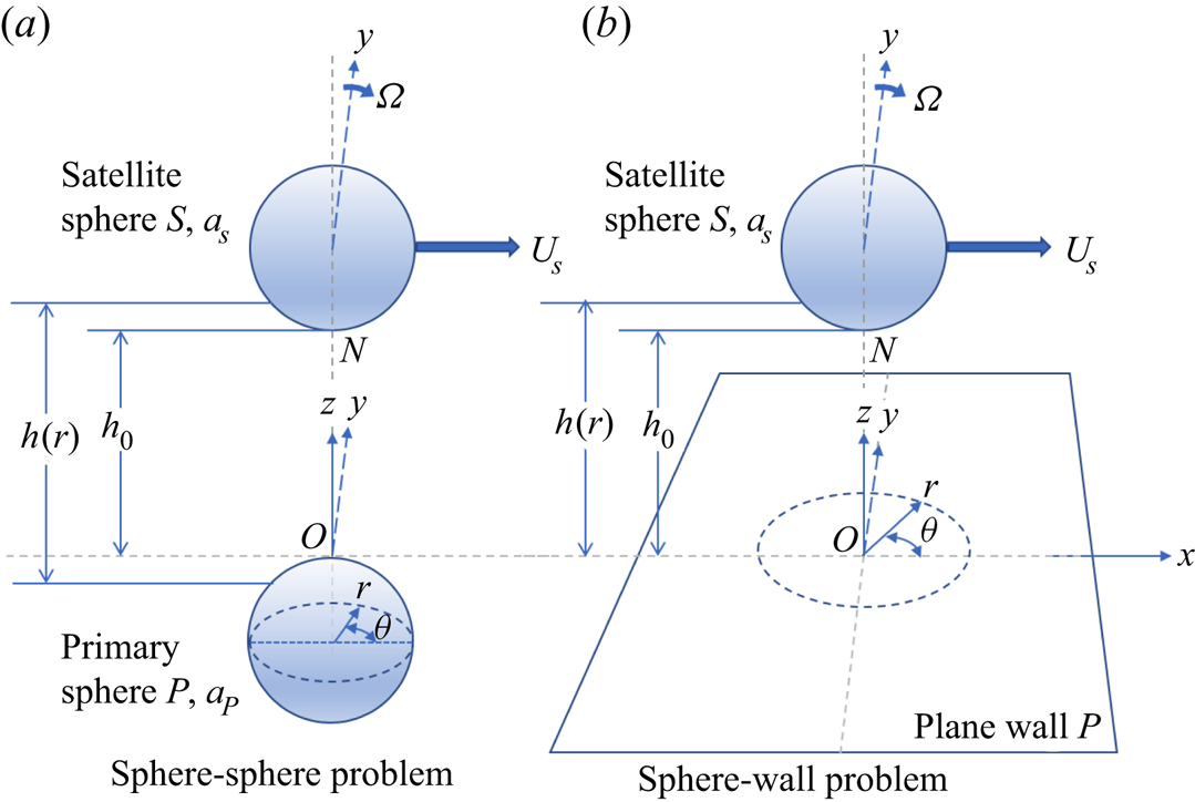
Figure 1 shows a sketch of the two spheres. We designate sphere ‘ $P$’ as the ‘primary’ sphere and sphere ‘
 $S$’ as the ‘satellite’ sphere. We consider the fluid motion generated by the translation and rotation of sphere S relative to sphere
 $P$ at rest at the origin. The fluid is an infinite gas with a density
 $\rho$ and viscosity
 $\mu$. Defining the radii of the primary and satellite spheres as
 $a_P$ and
 $a_S$, respectively, the harmonic mean radius is
 \begin{equation} a =\frac{a_Sa_P}{a_S+a_P} . \end{equation}
As we are concerned with tangential HI, we consider sphere  $S$ moving with translational velocity of (
 $U_S,0,0$) and angular velocity of (
 $0,a_S\varOmega ,0$) in Cartesian coordinates.
Sketch in isometric view of the sphere  $S$ in cylindrical coordinates with the minimum gap separation
 $h_0$ measured from the nearest point
 $N$ on
 $S$ to the origin
 $O$ on sphere
 $P$ (a) and on plane
 $P$ (b).

We assume the Reynolds and Mach numbers of the flow are vanishingly small allowing us to neglect fluid inertia and use results obtained from the linearized Boltzmann equation, treating incompressibility as discussed in Gopinath et al. (Reference Gopinath, Chen and Koch1997). As we are concerned with non-continuum effects at small separations, we introduce the Knudsen number defined as  $Kn\equiv \lambda /a$, where recall
 $\lambda$ is the mean free path of the gas. The analysis will be restricted to the large sphere limit,
 $Kn\ll 1$. The non-dimensional parameter characterizing the separation of the spheres is defined as
 $\varepsilon \equiv h_0/a$, where
 $h_0$ is the minimum separation distance of the sphere surfaces (see figure 1). In terms of the non-continuum analysis, the relevant non-dimensional separation is given by
 $\delta _0\equiv h_0/\lambda$. Note that, by definition,
 $\varepsilon = \delta _0 Kn$, which implies
 $\varepsilon \ll \delta _0$.
2.1. Spheres widely separated
For  $\delta _0\gg 1$, the governing equations for the fluid are the Stokes equation and continuity
 \begin{equation} \boldsymbol{\nabla} p = \mu \nabla^{2} \boldsymbol{u}, \quad \boldsymbol{\nabla}\boldsymbol{\cdot}\boldsymbol{u} = 0, \end{equation}
where  $\boldsymbol{u}$ is the fluid velocity and p is the pressure.
Figure 1 shows the cylindrical coordinate system that will be used to analyse the flow in the gap. In cylindrical coordinates ( $r,\theta ,z$), the dimensional gap separation
 $h(r)$ with minimum gap separation
 $h_0$ is given by
 \begin{equation} h(r) = h_0 + \left(a_S-\sqrt{a_S^{2}-r^{2}}\right) + \left(a_P-\sqrt{a_P^{2}-r^{2}}\right). \end{equation}
For  $\varepsilon \ge O(1)$, the disturbance velocity field of a sphere can be written as a multipole expansion about its centre (Kim & Karrila Reference Kim and Karrila1991). The leading-order terms for the far field can be calculated by the method of reflections, but this becomes computationally expensive, as the number of terms required for a given accuracy increases with decreasing separation. Jeffrey & Onishi (Reference Jeffrey and Onishi1984) developed the twin multipole expansion method that expresses Lamb's solution expanded with respect to two different origins. The result is a tractable means for computing the HIs of two spheres of arbitrary size ratio down to separations as small as
 $\varepsilon \gtrsim 0.1$.
2.2. Spheres in near contact
In the limit  $\varepsilon \ll 1$ and
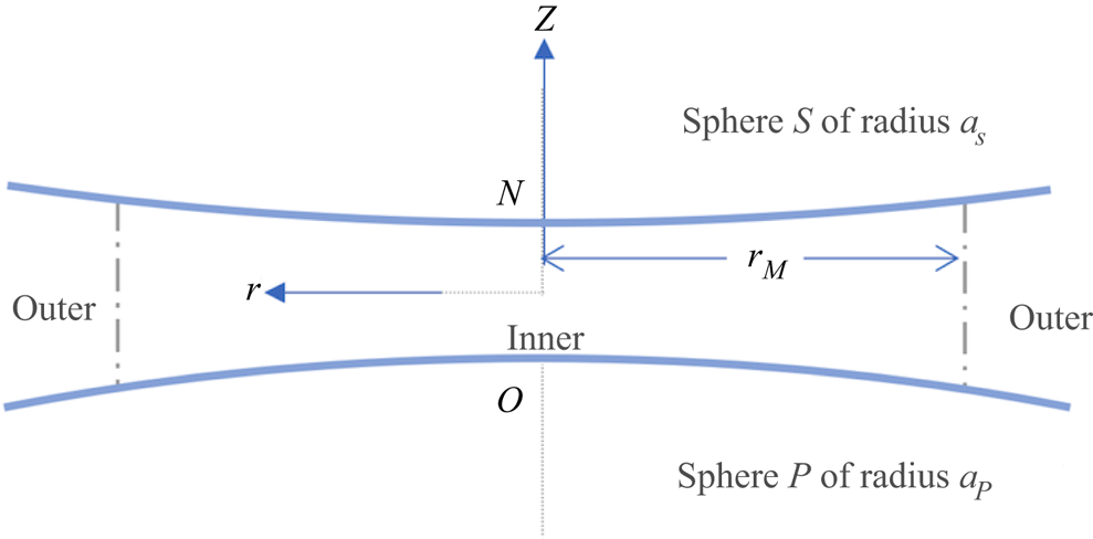
 $\delta _0\gg 1$, the continuum flow in the gap obeys the Stokes equation and can be analysed using a matched asymptotic analysis. O'Neill & Stewartson (Reference O'Neill and Stewartson1967) identified an ‘inner region’, where they applied the standard lubrication approximation, and an ‘outer region’, where the full Stokes equations were used. The solutions are equated at a radial distance
 $r_{M}$. Figure 2 depicts the ‘inner’ and ‘outer’ regions. In the inner region, we are interested in the limit
 $r\ll a_P$ and
 $r\ll a_S$, allowing us to introduce a Taylor series expansion for the two square roots in (2.3), yielding
 \begin{align} h(r) = h_0 + a_S\left[1- \left(1-\frac{1}{2a_S^{2}}r^{2}-\frac{1}{8a_S^{4}}r^{4}\ldots\right) \right] \!+ a_P\left[1\!- \left(1\!-\frac{1}{2a_P^{2}}r^{2}\!-\frac{1}{8a_P^{4}}r^{4}\ldots\right) \right]. \end{align}
Rearranging (2.4) and introducing (2.1) yields
 \begin{equation} \frac{h(r)}{h_0} =1+ \frac{1}{2} \left( \frac{1}{ah_0} \right)r^{2} + \frac{1}{8} \left( \frac{1}{ah_0} \right)^{2} r^{4}\ldots. \end{equation}
The independent variables are made dimensionless as
 \begin{equation} R\equiv\frac{r}{\sqrt{a h_0}} ,\quad Z\equiv\frac{{z}}{h_0} . \end{equation}
To leading order, the dimensionless gap of (2.5) is expressed as
 \begin{equation} H(R)\equiv\frac{h(r)}{h_0} = 1 + \frac{1}{2}R^{2}. \end{equation}
The equations defining the surfaces of the two spheres are then defined as
 \begin{equation} \left. \begin{gathered} Z_S = 1 + \tfrac{1}{2}\alpha R^{2}, \\ Z_P ={-}\tfrac{1}{2}(1-\alpha)R^{2}, \end{gathered} \right\} \end{equation}
where  $\alpha$ is the size ratio
 \begin{equation} \alpha\equiv\frac{a}{a_S} , \end{equation}
and consequently  $\alpha \rightarrow 1$ for
 $a_P/a_S\rightarrow \infty$ and
 $\alpha \rightarrow 0$ for
 $a_S/a_P\rightarrow \infty$.
Sketch of the inner region defined as  $0<r<r_{M}$ and outer region defined as
 $r>r_{M}$.

The velocity components and pressure can be written as (O'Neill & Stewartson Reference O'Neill and Stewartson1967)
 \begin{equation} \left. \begin{gathered} u_r(r,\theta,{z}) = U_S\; U(R,Z)\cos\theta, \\ u_\theta(r,\theta,{z}) = U_S\; V(R,Z)\sin\theta, \\ u_z(r,\theta,{z}) = U_S\; W(R,Z)\cos\theta, \\ p(r,\theta,{z}) = \frac{\mu U_S}{a} P(R,Z)\cos\theta, \end{gathered} \right\} \end{equation}
where U, V and W are the dimensionless velocity components and P is the dimensionless pressure. The resulting dimensionless governing equations become
 \begin{equation} \left. \begin{gathered} \varepsilon^{3/2} \frac{\partial P}{\partial R} ={-}\varepsilon \left[\frac{2(U+V)}{R^{2}} +\frac{\partial^{2} U}{\partial R^{2}} \right] + \frac{\partial^{2} U}{\partial Z^{2}},\\ -\varepsilon^{3/2}\frac{P}{R} ={-}\varepsilon\frac{ 2(U+V)}{R^{2}} + \frac{\partial^{2} V}{\partial Z^{2}},\\ \varepsilon^{3/2}\frac{\partial P}{\partial Z} = \varepsilon^{3/2} \left[ \frac{\partial^{2} W}{\partial R^{2}} +\frac{1}{R}\frac{\partial W}{\partial R} -\frac{W}{R^{2}} \right] + \varepsilon^{1/2} \frac{\partial^{2} W}{\partial Z^{2}} \end{gathered} \right\} \end{equation}
and the continuity equation is
 \begin{equation} \frac{\partial U}{\partial R} + \frac{U+V}{R} + \frac{1}{\varepsilon^{1/2}}\frac{\partial W}{\partial Z} = 0. \end{equation}
Equation (2.12) implies that both  $U$ and
 $V$ are
 $O(1)$ and
 $W$ is order
 $\varepsilon ^{1/2}$. It follows from (2.11) that the pressure,
 $P$, scales as
 $\varepsilon ^{-3/2}$. A regular expansion in
 $\varepsilon$ is then assumed to take the form
 \begin{equation} \left. \begin{gathered} U(R,{Z}) = U_0(R,{Z}) + \varepsilon U_1(R,{Z}) + \ldots,\\ V(R,{Z}) = V_0(R,{Z}) + \varepsilon V_1(R,{Z}) + \ldots,\\ W(R,{Z}) = \varepsilon^{1/2} W_0(R,{Z}) + \varepsilon^{3/2} W_1(R,{Z}) + \ldots,\\ P(R,{Z}) = \varepsilon^{{-}3/2} P_0(R,{Z}) + \varepsilon^{{-}1/2} P_1(R,{Z}) + \ldots.\end{gathered} \right\} \end{equation}
To leading order, the governing equations (2.11) and (2.12) become
 \begin{gather} \frac{\partial P_0}{\partial R} = \frac{\partial^{2} U_0}{\partial Z^{2}} ,\quad -\frac{P_0}{R} = \frac{\partial^{2} V_0}{\partial Z^{2}} , \quad \frac{\partial P_0}{\partial Z} = 0, \end{gather}
 \begin{gather} \frac{\partial U_0}{\partial R} + \frac{U_0+V_0}{R} + \frac{\partial W_0}{\partial Z} = 0. \end{gather}
3. Non-continuum flow analysis
For separation distances below the mean free path, i.e.  $\delta _0\le O(1)$, non-continuum effects become important and the Stokes equation (cf. 2.2a,b) is no longer a valid representation of the inner flow. The continuity equation continues to hold for a non-continuum gas whose pressure variation is small compared to the ambient pressure, as do the
 $\varepsilon$ scalings in (2.10), except the variables are functions of
 $\delta _0$ too. To analyse the non-continuum velocity and pressure, we replaced the Stokes equation for the inner region of the lubrication layer with the BGK approximation to the linearized Boltzmann equation (Bhatnagar et al. Reference Bhatnagar, Gross and Krook1954). As shown in § 3.1, we employ BGK solutions for Poiseuille and Couette flows from the literature to construct the inner solution for the lubrication layer. Note that, because we assume
 $Kn\ll 1$, the outer flow is in the continuum regime even when the inner flow is not (all the way up to contact), simplifying the matching process.
3.1. Decomposition of the lubrication flow
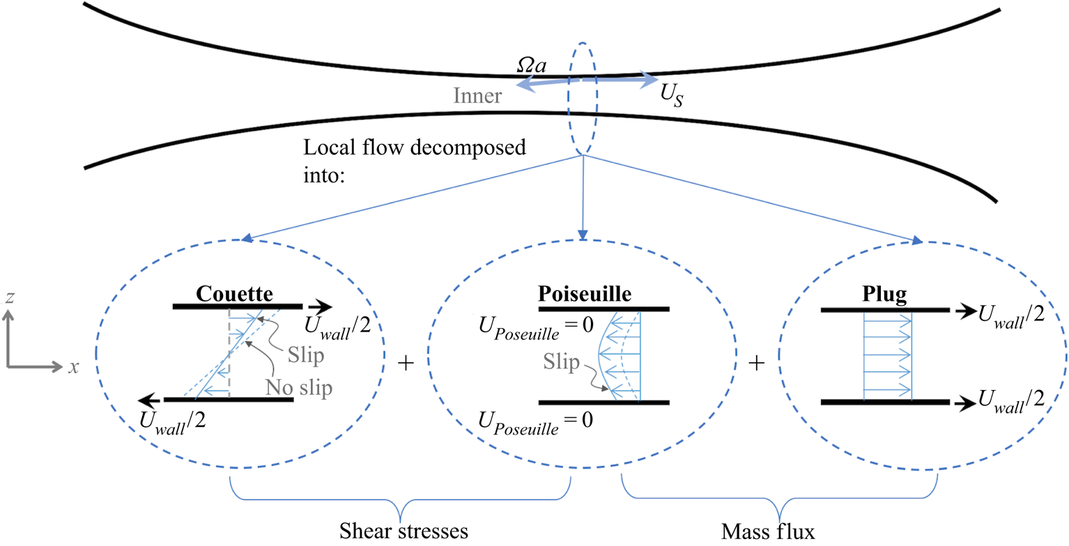
Under the standard lubrication approximation, the local flow between the two spheres can be represented as a superposition of Poiseuille, Couette and plug flows, as depicted in figure 3. Poiseuille flow is characterized by the pressure gradient driving the flow, whereas Couette flow is characterized by the shear rate between the two surfaces. Plug flow assumes a uniform velocity across the channel. Its role is to allow arbitrary boundary conditions to be satisfied. Poiseuille and plug flows contribute to the mass flux through the gap while Poiseuille and Couette flows contribute to the shear stress on the sphere surfaces. The weights associated with the Couette and plug flows are determined by the boundary conditions.
Sketch of the inner region in the xz plane decomposed into three planar flows: Couette, Poiseuille and plug flows. The Poiseuille flow depends upon the pressure gradient, the mass flux is determined by the plug and Poiseuille flows, and the shear stresses are obtained from the Poiseuille and Couette flows.

Recall this study is concerned with the forces and torques associated with tangential motions of the spheres. In the Cartesian coordinate system shown in figure 1, the tangential motion between the spheres arises from a combination of translation of sphere S in a direction perpendicular to the line of centres, given by ( $U_S,0,0$), and its rotation along an axis perpendicular to the line of centres, defined as (
 $0,\varOmega a_S,0$). The resulting
 ${x}$ velocity of the surface of sphere S,
 $U_{wall}$ (see figure 3), can be approximated in the inner region as
 \begin{equation} U_{{wall}} = U_{{S}} (1 - \omega), \end{equation}
where
 \begin{equation} \omega = \frac{ \varOmega a_S}{U_{{S}}}. \end{equation}
Below, we show how the boundary conditions are used to obtain the weighting of Couette and plug flows. However, first we must account for the non-continuum Poiseuille and Couette flows in the gap.
3.1.1. Poiseuille flow
Cercignani & Daneri (Reference Cercignani and Daneri1963) analysed the pressure-driven flow of a rarefied gas between two parallel plates using the BGK model (Bhatnagar et al. Reference Bhatnagar, Gross and Krook1954). For consistency with the analysis for spheres given below, we designate the separation distance between the plates  $h$ and the dimensionless separation,
 $\delta = h/\lambda$. The volumetric flux, defined as the average velocity integrated across the channel, is proportional to the average pressure gradient in all regimes, i.e. the pseudo-free molecular regime (
 $\delta \ll 1$), transition (
 $\delta = O(1$)) and continuum regime (
 $\delta \gg 1$). The general dimensionless expression is given by
 \begin{equation} \int_0^{1} U(Z)\,\textrm{d}Z ={-} \frac{g(\delta)}{2\delta} \frac{\textrm{d}P}{\textrm{d}X}, \end{equation}
where we apply the same scaling as described in § 2.2 and  $g(\delta )$ is a dimensionless function that accounts for the transitions through the different regimes. The limit
 $\delta \ll 1$ corresponds to the pseudo-free molecular regime, where
 $g(\delta )$ has an analytical form. Likewise in the limit
 $\delta \gg 1$, the solution approaches the Hagen Poiseuille law with a slip coefficient,
 $k_1= 1.016$ (see § 3.4 for a definition and more complete explanation of the slip coefficient). In the transition regime, the values were numerically evaluated and tabulated by Cercignani & Daneri (Reference Cercignani and Daneri1963). The resulting expression for
 $g(\delta )$ is
 \begin{equation} g(\delta)= \left\{ \begin{array}{@{}ll} -\dfrac{1}{\sqrt{\rm \pi}}(-\ln\delta +0.8), & (\delta<0.01),\\ V(\delta), & (0.01<\delta<10),\\ \dfrac{\delta}{6}+ k_1, & (\delta>10), \end{array} \right. \end{equation}
where  $\delta < 0.01$ corresponds to the pseudo-free molecular regime,
 $\delta > 10$ corresponds to the continuum flow regime and
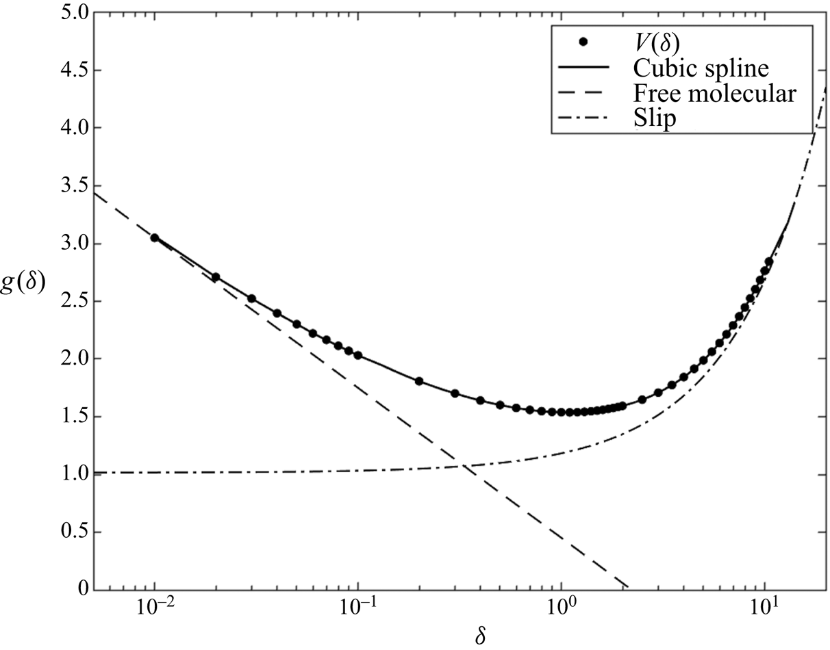
 $V(\delta )$ represents a curve fit of the tabulated results from Cercignani & Daneri (Reference Cercignani and Daneri1963). Figure 4 shows a plot of
 $g(\delta )$. The markers (
 $\bullet$) are the tabulated values, the solid line is the cubic spline fit, and the limiting solutions for the pseudo-free molecular and continuum regimes are the dashed and dash-dot lines, respectively.
The  $g(\delta )$ function (3.4) showing the tabulated results of Cercignani & Daneri (Reference Cercignani and Daneri1963) (
 $\bullet$), the cubic spline fit used to interpolate between the points (line) and the limiting solutions for the pseudo-free molecular (dashed line) and slip (dash-dot line) regimes.

3.1.2. Couette flow
In the case of planar Couette flow, the variable of interest is the shear stress in terms of the velocity difference between the top and bottom walls. Linearity and symmetry imply that the normal stress differences in low-Mach-number non-continuum planar Couette flow are zero, just as they are for low-Reynolds-number continuum Couette flow. We consider the motion of a rarefied gas between two parallel plates separated by a distance,  $h$, with the top plate moving with a velocity
 $U_{wall}/2$ and the bottom plate moving with a velocity
 $-U_{wall}/2$, creating a velocity difference across the channel of
 $U_{wall}$. In the free molecular limit (i.e.
 $\delta = h/\lambda \rightarrow 0$), the linearized Boltzmann equation can be solved analytically for small Mach number (Kogan Reference Kogan1969). The velocity of the rarefied gas in this limit is constant over the gap and equal to the arithmetic mean of the wall velocities such that the dimensional free molecular shear stress
 $\tau _{{xz}}^{{fm}}$ in the
 ${xz}$ plane is given by
 \begin{equation} \tau_{{{xz}}}^{{fm}} ={-}\frac{\mu U_{wall}}{\sqrt{\rm \pi} \lambda }, \end{equation}
where  $\mu = (1/2) \rho c \lambda$ is the molecular viscosity,
 $c = \sqrt {2p/\rho }$ is the mean molecular speed,
 $\rho$ is the density and
 $p$ is the thermodynamic pressure. Sharipov (Reference Sharipov2016) used the method of successive approximations based on the linearized Boltzmann equation to obtain the first order correction to the stress for small values of
 $\delta$. If we non-dimensionalize the stress with the free molecular stress in (3.5), the resulting expression is
 \begin{equation} \frac{\tau_{{{xz}}}}{\tau_{{{xz}}}^{{fm}}} = 1 - \frac{\sqrt{\rm \pi}}{2} \delta. \end{equation}
In the continuum limit (i.e.  $\delta \gg 1$), the solution approaches the Couette solution with slip boundary conditions
 \begin{equation} \frac{\tau_{{{xz}}}}{\tau_{{{xz}}}^{{fm}}} = \frac{\sqrt{\rm \pi}}{\delta + 2 k_1} , \end{equation}
where once again  $k_1$ is the slip coefficient.
In the transition region, Cercignani & Pagani (Reference Cercignani and Pagani1966) solved the linearized Boltzmann equation using a variational principle with cutoff points approaching the limits. We can define a comprehensive expression for the stress across all regimes by introducing the dimensionless function  $\eta (\delta )$, defined as
 \begin{equation} \eta(\delta) = \frac{ \tau_{{{xz}}}}{\tau_{{{xz}}}^{{fm}}}, \end{equation}
which takes the form
 \begin{equation} \eta(\delta)= \left\{
\begin{array}{@{}ll} 1 - \dfrac{\sqrt{\rm \pi}}{2}\delta, &
(\delta<0.1),\\ Y(\delta), & (0.1<\delta<10),\\
\dfrac{\sqrt{\rm \pi}}{\delta+2k_1}, & (\delta>10),
\end{array} \right. \end{equation}
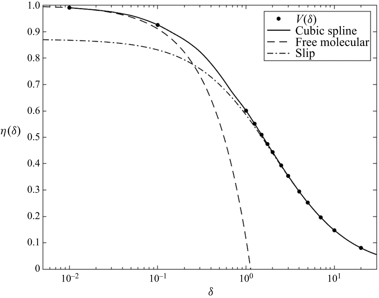
where  $Y(\delta )$ is a cubic spline fit of the tabulated values obtained by Cercignani & Pagani (Reference Cercignani and Pagani1966). The plot of
 $\eta (\delta )$ as a function of
 $\delta$ is shown in figure 5. The markers (
 $\bullet$) are the tabulated values, the solid line is the cubic spline fit, and the limiting solutions for the free molecular and continuum regimes are the dashed and dash-dot lines, respectively.
The  $\eta (\delta )$ function (3.9) showing the tabulated results of Cercignani & Pagani (Reference Cercignani and Pagani1966) (
 $\bullet$), the cubic spline fit used to interpolate between the points (line) and the limiting solutions for the free molecular (dashed line) and slip (dash-dot line) regimes.

Lastly, we note that there are no non-continuum effects to plug flow. So the above solutions for Poiseuille and Couette flows are all that we need to define the inner solution to the lubrication analysis. The next section discusses how the pressure field in the gap between the spheres is determined.
3.2. Inner pressure field
Sundararajakumar & Koch (Reference Sundararajakumar and Koch1996) extended the results of Cercignani & Daneri (Reference Cercignani and Daneri1963) to include the effects of curvature so that the analysis could be applied to the inner region of the lubrication flow between the spheres. The approach taken here is identical except now applied to the translation of sphere  $S$ in the
 ${x}$-direction and rotation along the
 ${y}$-axis, i.e. perpendicular to the line of centres. The flow in the gap is represented locally as a superposition of Couette, Poiseuille and plug flows. However, because of curvature, the resulting velocity is two-dimensional. Integrating the continuity equation (2.15) across the gap yields
 \begin{equation} \int_{Z_P}^{Z_S} \frac{\partial U_0}{\partial R} \,\textrm{d}Z + \frac{1}{R}\int_{Z_P}^{Z_S}(U_0 + V_0) \,\textrm{d}Z + \int_{Z_P}^{Z_S} \frac{\partial W_0}{\partial Z} \,\textrm{d}Z = 0. \end{equation}
The final term can be evaluated in terms of the kinematic boundary condition at the two sphere surfaces, which can be written as
 \begin{equation} W_0(R,Z_P) = 0, \quad W_0(R,Z_S) = [(U_0(R,Z_S)-1)]\alpha R . \end{equation}
We rewrite the first term in (3.10) using Leibniz's rule
 \begin{equation} \int_{Z_P}^{Z_S} \frac{\partial U_0}{\partial R} \,\textrm{d}Z = \frac{\textrm{d}}{\textrm{d}R}\left(\int_{Z_P}^{Z_S} U_0 \,\textrm{d}Z\right) - U_0(R,Z_S)\frac{\textrm{d} Z_S}{\textrm{d}R} + U_0(R,Z_P)\frac{\textrm{d} Z_P}{\textrm{d}R}. \end{equation}
Introducing the variable change
 \begin{equation} \tilde{x} = \tfrac{1}{2} R^{2} \quad\rightarrow\quad {\textrm{d}\tilde{x}} = R\,\textrm{d}R, \end{equation}
(3.10) is then written as
 \begin{equation} \frac{\textrm{d}}{\textrm{d}\tilde{x}}\left(\int_{Z_P}^{Z_S} U_0\, \textrm{d}Z\right) + \frac{1}{2\tilde{x}} \int_{Z_P}^{Z_S} (U_0 + V_0)\,\textrm{d}Z - \alpha = 0 . \end{equation}
Note that the integrated continuity result shown in (3.14), expressed in terms of the mass flux through the lubrication gap, is solely due to the kinematic boundary condition at the solid surfaces and is not altered by the slip of the gas at the surfaces.
Recall that we decompose the velocities  $U_0$ and
 $V_0$ into a sum of Poiseuille, Couette and plug flows, denoted by superscripts
 $p, c, g$ respectively, yielding
 \begin{equation} \left. \begin{gathered} U_0 = U^{p}_0 + U^{c}_0 + U^{g}_0, \\ V_0 = V^{p}_0 + V^{c}_0 + V^{g}_0. \end{gathered} \right\} \end{equation}
The pressure field is related to the flux through the gap. To leading order, the pressure is uniform across the gap (i.e.  $\partial P_0/\partial Z = 0$). Generalizing (3.3) to the two-dimensional flow within the gap, the relations for the integral of velocities
 $U^{p}_0$ and
 $V^{p}_0$ are (Cercignani & Daneri Reference Cercignani and Daneri1963)
 \begin{gather} \int_{Z_P}^{Z_S} U^{p}_0\, \textrm{d}Z ={-}\frac{1}{2} \frac{\delta^{2}}{\delta_0^{3}} g(\delta) \frac{\partial P_0}{\partial R}, \end{gather}
 \begin{gather} \int_{Z_P}^{Z_S} V^{p}_0\, \textrm{d}Z = \frac{1}{2} \frac{\delta^{2}}{\delta_0^{3}} g(\delta) \frac{P_0}{R}. \end{gather}
Couette flow does not contribute to the flux
 \begin{equation} \int_{Z_P}^{Z_S} U^{c}_0\, \textrm{d}Z = \int_{Z_P}^{Z_S} V^{c}_0\, \textrm{d}Z = 0, \end{equation}
and for plug flow the integrals of the velocities are
 \begin{equation} \int_{Z_P}^{Z_S} U^{g}_0\, \textrm{d}Z ={-} \int_{Z_P}^{Z_S} V^{g}_0\, \textrm{d}Z = \tfrac{1}{2}(1-\omega). \end{equation}
Substituting these expressions into (3.14) yields a differential equation for the non-continuum pressure. To simplify the result, we introduce the notation
 \begin{equation} \tilde q= \frac{P_0}{R} . \end{equation}
Notice that only the integrals of the velocities due to Poiseuille flow contain the pressure, while (3.19) can be combined with the ‘ $\alpha$’ in (3.14) to give
 $(2\alpha - 1 + \omega )$. Factoring that quantity out of (3.14) yields the following
 \begin{equation} 2\tilde{x}\delta^{2} g q'' + \left[2\tilde{x} \frac{\textrm{d}(\delta^{2} g)}{\textrm{d}\tilde{x}} + 4\delta^{2} g \right] q'+ \frac{\textrm{d}(\delta^{2} g)}{\textrm{d}\tilde{x}} q ={-}\delta_0^{3} , \end{equation}
where
 \begin{equation} \left. \begin{gathered} q' \equiv \dfrac{\textrm{d}q}{\textrm{d}\tilde{x}} = \frac{1}{R^{2}}\frac{\partial P_0}{\partial R} -\frac{P_0}{R^{3}} ,\\ q'' \equiv \dfrac{\textrm{d}^{2} q}{{\textrm{d}\tilde{x}}^{2}} =\frac{1}{R^{3}}\frac{\partial^{2} P_0}{\partial R^{2}} - \frac{3}{R^{4}}\frac{\partial P_0}{\partial R} + \frac{3P_0}{R^{5}} , \end{gathered} \right\} \end{equation}
and  $q$ is
 $\tilde {q}$ rescaled as follows to separate translational and rotational motions
 \begin{equation} \tilde{q} = q (2 \alpha - 1 + \omega). \end{equation}
In the limit of pure translation,  $\omega \rightarrow 0$ and therefore
 $\tilde {q} = q(2 \alpha -1)$. In the limit of pure rotation,
 $\omega \rightarrow \infty$ ,
 $\tilde {q} = q \omega$ and from (2.10) the pressure is rescaled as
 $p = \mu \varOmega P \cos \theta$. Note that the definition of
 $q$ precisely eliminates the singularity (at
 $r = 0$) in the differential equation. The numerical solution for
 $q$ of interest is finite at
 $\tilde{x} = 0$ and asymptotes to the continuum pressure
 $q_\infty$ as
 $\tilde{x} \rightarrow \infty$ (O'Neill & Majumdar Reference O'Neill and Majumdar1970)
 \begin{equation} q_\infty = \tfrac{1}{5 H^{2}} . \end{equation}
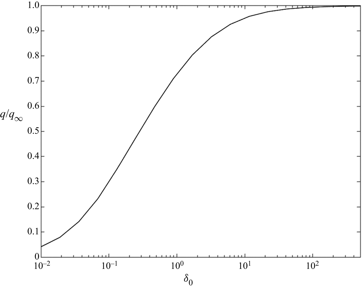
The ratio of the non-continuum pressure to the continuum pressure as a function of  $\delta _0$ is shown in figure 6.
Graph of non-continuum pressure normalized by the continuum pressure on the axis between the centres plotted against rarefied parameter  $\delta _0$.

3.3. Force and torque from inner region
The force exerted by the fluid in the inner region of the surface of the particles is comprised of the force due to pressure (Poiseuille flow) and the force arising from the shear stresses (Poiseuille and Couette flows).
The force due to pressure is calculated by integrating minus the pressure times the unit outward normal on the surface,  $\boldsymbol {n}_P$ and
 $\boldsymbol {n}_S$ for spheres
 $P$ and
 $S$, respectively, over the sphere surface. The unit normals can be approximated as
 \begin{equation} \left. \begin{gathered} \boldsymbol{n}_P = \boldsymbol{e}_{{z}} + \frac{r}{a_P}\sin\theta\; \boldsymbol{e}_{{y}} + \frac{r}{a_P}\cos\theta\ \boldsymbol{e}_{{x}} ,\\ \boldsymbol{n}_S ={-} \boldsymbol{e}_{{z}} + \frac{r}{a_S}\sin\theta\; \boldsymbol{e}_{{y}} + \frac{r}{a_S}\cos\theta\ \boldsymbol{e}_{{x}}, \end{gathered} \right\} \end{equation}
where  $\boldsymbol {e}_{{x}}$,
 $\boldsymbol {e}_{{y}}$ and
 $\boldsymbol {e}_{{z}}$ are unit normals pointing in the
 ${x}$,
 ${y}$ and
 ${z}$ directions, respectively. Recall the pressure to leading order in
 $\varepsilon$ can be expressed as
 \begin{equation} p(r,\theta,{{z}}) = \varepsilon^{{-}3/2} \frac{\mu U_S}{a} P_0(R) \cos\theta , \end{equation}
where  $P_0(R)$ is determined by integrating (3.21) and using the relationships
 $P_0 = \tilde {q} \sqrt {2\tilde{x}}$ and
 $\tilde{x} = R^{2}/2$. We are interested in the contribution to the force acting in the
 ${x}$-direction (i.e. tangential), which is obtained by integrating minus the pressure times the
 ${x}$ component of the unit normal over the surface of both spheres. Because the pressure acts normal to the sphere surfaces it produces no torque on the spheres. The result is
 \begin{equation} - \int_0^{r_M} \int_0^{2{\rm \pi}} p \boldsymbol{n}_P \boldsymbol{\cdot} \boldsymbol{e}_{x}\, \mathrm{d} \theta\ r\, \mathrm{d}r ={-}6{\rm \pi}\mu U_S a (2\alpha-2) \int_0^{\tilde{x}_M} \tilde{x} \tilde{q}\, \mathrm{d}\tilde{x}. \end{equation}
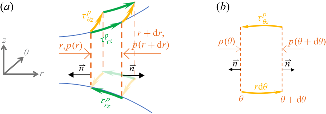
A momentum balance on the inner region is used to construct the components of the shear stress due to Poiseuille flow in the  $r{z}$ and
 $\theta {z}$ planes, as shown in figure 7. The resulting expressions are
 \begin{gather} \tau^{p}_{r{{z}}} = \frac{1}{2} h(r) \frac{\partial p}{\partial r} , \end{gather}
 \begin{gather}\tau^{p}_{\theta {{z}}} = \frac{1}{2}\frac{h(r)}{r}\frac{\partial p}{\partial\theta} , \end{gather}
where the superscript ‘ $p$’ indicates the shear stress due to Poiseuille flow and the subscripts are the coordinate directions. Resolving the stress acting in the
 $x$ direction yields
 \begin{equation} \tau^{p}_{{x{z}}} = \tau^{p}_{r{{z}}} \cos\theta - \tau^{p}_{\theta {{z}}} \sin\theta . \end{equation}
Substituting (3.26) and integrating the result over the sphere surfaces allows us to calculate the force and torque due to the shear stress from Poiseuille flow.
Momentum balance in the  $r{z}$ plane (a) and in the
 $\theta {z}$ plane (b) due to Poiseuille flow only in the local gap in cylindrical polar coordinates.

Finally, we consider the shear stress due to Couette flow in the gap, which can be written as (cf. (3.5), (3.8) and (3.9))
 \begin{equation} \tau^{c}_{{x{z}}} ={-}\frac{\mu U_{wall}}{\sqrt{\rm \pi} h_0}\delta_0\eta(\delta) , \end{equation}
where the superscript ‘ $c$’ indicates the shear stress due to Couette flow. Integrating this quantity over the surface of the two spheres enables the calculation of the force and torque due to the shear stress from Couette flow.
We obtain the total force acting on each sphere in the tangential ( $x$) direction by summing the contribution from the pressure (Poiseuille flow) and shear stresses (Poiseuille and Couette flows). Likewise, we can compute the total torque by summing the contributions due to the Poiseuille and Couette stresses. The tangential force and torque acting on a sphere due to its translation and rotation are non-dimensionalized as follows
 \begin{gather} \hat{f}^{{\perp}}_{t,i} = \frac{F^{{\perp}}_{t,i}}{-6{\rm \pi}\mu a U_S},\quad \hat{f}^{{\perp}}_{r,i} = \frac{F^{{\perp}}_{r,i}}{-6{\rm \pi}\mu a (a_S \varOmega)} , \end{gather}
 \begin{gather} \hat{t}^{{\perp}}_{t,i} = \frac{T^{{\perp}}_{t,i}}{-8{\rm \pi}\mu a a_i U_S},\quad \hat{t}^{{\perp}}_{r,i} = \frac{T^{{\perp}}_{r,i}}{-8{\rm \pi}\mu a a_i (a_S \varOmega)} , \end{gather}
where the subscript  $i$ refers to sphere
 $P$ or
 $S$ and the hat above the variable indicates the contribution from the inner region.
Integrating the radial direction up to the non-dimensional radial distance  $R_{M}$, which lies in the range
 $\delta _0^{-1/2}\ll R_M\ll \varepsilon ^{-1/2}$, yields the following expressions for the dimensionless non-continuum inner forces and torques
 \begin{gather} \left. \begin{gathered} \hat{f}^{{\perp} {NC}}_{t,S} = \frac{1}{3\sqrt{\rm \pi}}\int_{\delta_0}^{\delta_{M}} \eta(\delta)\,\mathrm{d} \delta + (2\alpha-1)(\tilde{x}Hq)_{M} + (2\alpha - 1)^{2}\int_0^{\tilde{x}_{M}} \tilde{x}q\, \mathrm{d}\tilde{x},\\ \hat{f}^{{\perp} {NC}}_{t,P} ={-}\frac{1}{3\sqrt{\rm \pi}}\int_{\delta_0}^{\delta_{M}} \eta(\delta)\,\mathrm{d} \delta + (2\alpha-1)(\tilde{x}Hq)_{M} - (2\alpha - 1)^{2}\int_0^{\tilde{x}_{M}} \tilde{x}q\, \mathrm{d}\tilde{x},\\ \hat{f}^{{\perp} {NC}}_{r,S} ={-}\frac{1}{3\sqrt{\rm \pi}}\int_{\delta_0}^{\delta_{M}} \eta(\delta)\,\mathrm{d} \delta + (\tilde{x}Hq)_{M} + (2\alpha - 1)\int_0^{\tilde{x}_{M}} \tilde{x}q \,\mathrm{d}\tilde{x},\\ \hat{f}^{{\perp} {NC}}_{r,P} = \frac{1}{3\sqrt{\rm \pi}}\int_{\delta_0}^{\delta_{M}} \eta(\delta)\,\mathrm{d} \delta + (\tilde{x}Hq)_{M} - (2\alpha - 1)\int_0^{\tilde{x}_{M}} \tilde{x}q\, \mathrm{d}\tilde{x}, \end{gathered} \right\} \end{gather}
 \begin{gather} \left. \begin{gathered} \hat{t}^{{\perp}{NC}}_{t,S} ={-} \frac{1}{4\sqrt{\rm \pi}}\int_{\delta_0}^{\delta_{M}} \eta(\delta)\,\mathrm{d} \delta - \frac{3}{4}(2\alpha-1)(\tilde{x}Hq)_{M} + \frac{3}{4}(2\alpha - 1)\int_0^{\tilde{x}_{M}} \tilde{x}q \,\mathrm{d}\tilde{x},\\ \hat{t}^{{\perp} {NC}}_{t,P} ={-} \frac{1}{4\sqrt{\rm \pi}}\int_{\delta_0}^{\delta_{M}} \eta(\delta)\,\mathrm{d} \delta + \frac{3}{4}(2\alpha-1) (\tilde{x}Hq)_{M} - \frac{3}{4}(2\alpha - 1)\int_0^{\tilde{x}_{M}} \tilde{x}q\, \mathrm{d}\tilde{x}, \\ \hat{t}^{{\perp} {NC}}_{r,S} = \frac{1}{4\sqrt{\rm \pi}}\int_{\delta_0}^{\delta_{M}} \eta(\delta)\,\mathrm{d} \delta - \frac{3}{4}(\tilde{x}Hq)_{M} + \frac{3}{4}\int_0^{\tilde{x}_{M}} \tilde{x}q\, \mathrm{d}\tilde{x},\\ \hat{t}^{{\perp} {NC}}_{r,P} = \frac{1}{4\sqrt{\rm \pi}}\int_{\delta_0}^{\delta_{M}} \eta(\delta)\,\mathrm{d} \delta + \frac{3}{4}(\tilde{x}Hq)_{M} - \frac{3}{4}\int_0^{\tilde{x}_{M}} \tilde{x}q\, \mathrm{d}\tilde{x} , \end{gathered} \right\} \end{gather}
where  $\tilde{x}_{M} = R_{M}^{2}/2$,
 $\delta _{M}\equiv \delta _0(1+\tilde{x}_{M})$ and
 $(\tilde{x} H q)_{M}\equiv \tilde{x}_{M} (1 + \tilde{x}_{M}) q(\tilde{x}_{M})$. The superscript ‘
 $NC$’ is added to indicate the non-continuum inner solution. To complete the analysis, we supplement the inner contribution for the forces and torques with the outer contributions computed for continuum flow using a multipole solution to obtain an expression that is valid for all
 $\varepsilon$ in § 3.5. However, we first demonstrate that the non-continuum inner expressions derived herein are consistent with the classical analysis for a continuum fluid with ‘slip’ boundary conditions in § 3.4.
3.4. Relationship to classical slip analysis
The earliest work to introduce the first effects of the discrete nature of the gas was carried out by Hocking (Reference Hocking1973). For  $\delta _0\gg 1$, he modelled the flow using the continuum momentum equation, but replaced the no-slip boundary condition with the Maxwell slip boundary condition, as shown below for translational and rotational motions
 \begin{equation} \left. \begin{gathered} U_0(R, Z_P) - \beta\left. \frac{\partial U_0}{\partial Z} \right|_{Z_P}= V_0(R, Z_P) - \beta \left.\frac{\partial V_0}{\partial Z} \right|_{Z_P} = 0 ,\\ U_0(R, Z_S) + \beta \left.\frac{\partial U_0}{\partial Z} \right|_{Z_S} = V_0(R, Z_S) + \beta\left. \frac{\partial V_0}{\partial Z} \right|_{Z_S} = 1 - \omega, \end{gathered} \right\} \end{equation}
where  $\beta$ is the slip coefficient defined as
 \begin{equation} \beta \equiv \frac{k_1}{\delta_0} , \end{equation}
and recall  $k_1 = 1.016$ as predicted by the BGK theory (Loyalka & Ferziger Reference Loyalka and Ferziger1967).
We now show that this earlier analysis is consistent with the present work. The differential equation for the non-continuum pressure is shown in (3.21). If we replace  $g(\delta )$ by the form it takes in the slip regime,
 $g(\delta )=\delta /6 + k_1$, we obtain the following differential equation for the pressure, originally derived by Hocking (Reference Hocking1973)
 \begin{gather} 2\tilde{x} H^{2}(H + 6\beta) q_S'' + H[2\tilde{x}(3H + 12\beta) + 4H(H + 6\beta)] q_S' + H(3H + 12\beta) q_S ={-}1 , \end{gather}
where  $q_S$ indicates the continuum pressure with slip boundary conditions, scaled similarly as
 $\tilde q$ in (3.23). Likewise, substituting
 $\eta _S(\delta ) = \sqrt {{\rm \pi} }/(\delta + 2k_1)$ into the expressions for the force and torque given in (3.34) and (3.35), the inner resistivities reduce to the form derived by Hocking (Reference Hocking1973) (note that Hocking presented combined effects due to translational and rotational motions and defined the resistivity for torque with the opposite sign convention to this paper)
 \begin{gather} \left. \begin{gathered} \hat{f}^{{\perp} {S}}_{t,S} = \frac{1}{3}\ln\left(\frac{1+{\tilde{x}_{M}}+2\beta}{1+2\beta} \right) + (2\alpha-1) (\tilde{x}Hq_S)_{M} + (2\alpha-1)^{2}\int_0^{\tilde{x}_{M}}\tilde{x}q_S \,\mathrm{d}\tilde{x} ,\\ \hat{f}^{{\perp} {S}}_{t,P} ={-}\frac{1}{3}\ln\left(\frac{1+{\tilde{x}_{M}}+2\beta}{1+2\beta} \right) + (2\alpha-1) (\tilde{x}Hq_S)_{M} - (2\alpha-1)^{2}\int_0^{\tilde{x}_{M}}\tilde{x}q_S \,\mathrm{d}\tilde{x} ,\\ \hat{f}^{{\perp} {S}}_{r,S} ={-}\frac{1}{3}\ln\left(\frac{1+{\tilde{x}_{M}}+2\beta}{1+2\beta} \right) + (\tilde{x}Hq_S)_{M} + (2\alpha-1)\int_0^{\tilde{x}_{M}}\tilde{x}q_S\, \mathrm{d}\tilde{x} ,\\ \hat{f}^{{\perp} {S}}_{r,P} = \frac{1}{3}\ln\left(\frac{1+{\tilde{x}_{M}}+2\beta}{1+2\beta} \right) + (\tilde{x}Hq_S)_{M} - (2\alpha-1)\int_0^{\tilde{x}_{M}}\tilde{x}q_S\, \mathrm{d}\tilde{x} , \end{gathered} \right\} \end{gather}
 \begin{gather} \left. \begin{gathered} \hat{t}^{{\perp}{S}}_{t,S} ={-} \frac{1}{4}\ln\left(\frac{1\!+\!{\tilde{x}_{M}}\!+\!2\beta}{1\!+\!2\beta} \right) \!-\! \frac{3}{4}(2\alpha\!-\!1)(\tilde{x}Hq_S)_{M} \!+\! \frac{3}{4}(2\alpha-1)\int_0^{\tilde{x}_{M}}\tilde{x}q_S \,\mathrm{d}\tilde{x} ,\\ \hat{t}^{{\perp}{S}}_{t,P} ={-} \frac{1}{4}\ln\left(\frac{1\!+\!{\tilde{x}_{M}}\!+\!2\beta}{1\!+\!2\beta} \right) \!+\! \frac{3}{4}(2\alpha-1)(\tilde{x}Hq_S)_{M} \!-\! \frac{3}{4}(2\alpha-1)\int_0^{\tilde{x}_{M}}\tilde{x}q_S\,\mathrm{d}\tilde{x},\\ \hat{t}^{{\perp}{S}}_{r,S} \!=\! \frac{1}{4}\ln\left(\frac{1\!+\!{\tilde{x}_{M}}\!+\!2\beta}{1\!+\!2\beta} \right) \!-\! \frac{3}{4}(\tilde{x}Hq_S)_{M} \!+\! \frac{3}{4}\int_0^{\tilde{x}_{M}}\tilde{x}q_S\,\mathrm{d}\tilde{x} ,\\ \hat{t}^{{\perp}{S}}_{r,P} \!=\! \frac{1}{4}\ln\left(\frac{1\!+\!{\tilde{x}_{M}}\!+\!2\beta}{1\!+\!2\beta} \right) \!+\! \frac{3}{4}(\tilde{x}Hq_S)_{M} \!-\! \frac{3}{4}\int_0^{\tilde{x}_{M}}\tilde{x}q_S\,\mathrm{d}\tilde{x} , \end{gathered} \right\} \end{gather}
where the superscript ‘ $S$’ designates the continuum equations with slip boundary conditions. The above expressions differ from Hocking (Reference Hocking1973) in that the term
 $(\tilde{x}Hq_S)_{M}$ was approximated by
 $\tilde{x}^{2}_{M} q_S(\tilde{x}_{M})$; however, assuming
 $\tilde{x}_{M}\gg 1$, the difference is inconsequential.
The inner solution for the continuum equations with ‘no-slip’ boundary conditions are recovered by setting  $k_1=0$ and therefore
 $\beta =0$. The equation for the pressure reduces to
 \begin{equation} 2\tilde{x}H^{3} q_C'' + 2H^{2} (2H + 3\tilde{x}) q_C' + 3H^{2} q ={-}1 , \end{equation}
where  $q_C$ designates the continuum pressure with no-slip boundary conditions, scaled similarly as
 $\tilde q$ in (3.23). The result is consistent with the equation derived by O'Neill & Majumdar (Reference O'Neill and Majumdar1970) when written in terms of
 $P_0$ and
 $R$, and using their definition for the size ratio. A particular solution for this differential equation is
 \begin{equation} q_C = \frac{1}{5 H^{2}}. \end{equation}
Setting  $k_1=\beta =0$ and introducing (3.42) into (3.39) and (3.40) yields the inner contribution to the resistivity functions for the continuum equations with no-slip boundary conditions
 \begin{gather} \left. \begin{gathered} \hat{f}^{{\perp}{C}}_{t,S} = \left[\tfrac{1}{3} + \tfrac{1}{5} (2\alpha-1)^{2}\right] \ln(1+\tilde{x}_{M}) + \tfrac{2}{5}(1-\alpha)(2\alpha-1) ,\\ \hat{f}^{{\perp}{C}}_{t,P} = \left[-\tfrac{1}{3} - \tfrac{1}{5} (2\alpha-1)^{2}\right] \ln(1+\tilde{x}_{M}) + \tfrac{2}{5}\alpha(2\alpha-1) ,\\ \hat{f}^{{\perp}{C}}_{r,S} = \left[-\tfrac{1}{3} + \tfrac{1}{5} (2\alpha-1)\right] \ln(1+\tilde{x}_{M}) + \tfrac{2}{5}(1-\alpha) ,\\ \hat{f}^{{\perp}{C}}_{r,P} = \left[\tfrac{1}{3} - \tfrac{1}{5} (2\alpha-1)\right] \ln(1+\tilde{x}_{M}) + \tfrac{2}{5}\alpha , \end{gathered} \right\} \end{gather}
 \begin{gather} \left. \begin{gathered} \hat{t}^{{\perp}{C}}_{t,S} = \left[-\tfrac{1}{4} + \tfrac{3}{20}(2\alpha-1)\right] \ln(1+\tilde{x}_{M}) - \tfrac{3}{10}(2\alpha-1) , \\ \hat{t}^{{\perp}{C}}_{t,P} = \left[-\tfrac{1}{4} - \tfrac{3}{20}(2\alpha-1)\right] \ln(1+\tilde{x}_{M}) - \tfrac{3}{10}(2\alpha-1) ,\\ \hat{t}^{{\perp}{C}}_{r,S} = \tfrac{2}{5} \ln(1+\tilde{x}_{M}) - \tfrac{3}{10} , \\ \hat{t}^{{\perp}{C}}_{r,P} = \tfrac{1}{10} \ln(1+\tilde{x}_{M}) + \tfrac{3}{10} . \end{gathered} \right\} \end{gather}
The superscript ‘ $C$’ indicates these are solutions to the continuum equations with no-slip boundary conditions. O'Neill & Stewartson (Reference O'Neill and Stewartson1967) derived results for the pure translation of a sphere parallel to a plane, which corresponds to setting
 $\alpha =1$ yielding
 $\hat {f}^{\perp {C}}_{t,S} = 8(\ln (1 + \tilde{x}_{M}))/15$. Consistent with Jeffrey & Onishi (Reference Jeffrey and Onishi1984) and O'Neill & Stewartson (Reference O'Neill and Stewartson1967), the
 $O(1)$ term vanishes for
 $\alpha = 1$.
3.5. Uniformly valid solution
As discussed by O'Neill & Stewartson (Reference O'Neill and Stewartson1967), for a lubrication flow, the inner region corresponds to the domain where the pressure and velocity gradients are large and the lubrication approximation is valid. The inner solution will transition from the free molecular regime ( $\delta _0\ll 1$) to the continuum regime (
 $\delta _0\gg 1$) depending upon the value of
 $\delta _0$. As we are restricting this investigation to the limit
 $Kn\ll 1$ (recall the particle Knudsen number is defined as
 $Kn\equiv \lambda /a$), the outer flow, which scales with the sphere radius, will always be in the continuum regime, regardless of the regime of the inner flow. Hence the outer region is governed by the Stokes equation (2.2a,b). Complete solutions for the forces and torques are obtained by summing the contributions from the inner and outer regions.
To simplify the nomenclature, we will temporarily drop references to a particular resistivity, and define  $\hat {f}$ as the ‘inner’ contribution to a given resistivity and
 $\check {f}$ as the continuum ‘outer’ contribution to the same resistivity. The inner and outer solutions for a continuum fluid take the form
 \begin{equation} \left. \begin{gathered} \hat{f}^{C} = \hat{A}^{C}(\alpha) + B(\alpha)\ln\left(\frac{r_{M}}{h_0}\right) ,\\ \check{f} = \check{A}(\alpha) + B(\alpha)\ln\left(\frac{a}{r_{M}}\right), \end{gathered} \right\} \end{equation}
where the superscript ‘ $C$’ denotes the continuum inner solution,
 $r_{M}$ is the boundary between the inner and outer regions and
 $\hat {A}^{C}(\alpha )$,
 $\check {A}(\alpha )$ and
 $B(\alpha )$ are coefficients that depend on the size ratio,
 $\alpha$. Note that the functional form for the inner solution in (3.45) is taken from Jeffrey & Onishi (Reference Jeffrey and Onishi1984) for no-slip boundary conditions in the limit
 $\tilde{x}_{M}\gg 1$. The matched asymptotic solution for the continuum model of lubrication flow then takes the form (Jeffrey & Onishi Reference Jeffrey and Onishi1984; O'Neill & Majumdar Reference O'Neill and Majumdar1970)
 \begin{equation} f^{C} = \hat{f}^{C} + \check{f} = \hat{A}^{C}(\alpha) + \check{A}(\alpha) + B(\alpha)\ln\left(\frac{1}{\varepsilon}\right). \end{equation}
Notice that the dependence on  $r_{M}$ cancels out of the expression, so long as it lies within
 $(a h_0)^{1/2} \ll r_{M} \ll a$, where the approximations in (3.45) are valid.
Equations (3.34) and (3.35) have the following asymptotic form
 \begin{equation} \hat{f}^{NC} = \hat{A}^{NC}(\alpha, \delta_0) + B(\alpha)\ln\left(\frac{r_{M}}{h_0}\right). \end{equation}
The matched asymptotic expression for the uniformly valid resistivity for lubrication flow is then given by
 \begin{equation} f^{UV} = \hat{f}^{NC} + \check{f} = \hat{A}^{NC}(\alpha, \delta_0) + \check{A}(\alpha) + B(\alpha)\ln\left(\frac{1}{\varepsilon}\right) , \end{equation}
where the superscript ‘ $UV$’ refers to the uniformly valid lubrication flow solution corresponding to
 $\varepsilon \ll 1$ and
 $\delta _0 = O(1)$. Alternatively, the uniformly valid resistivity could be constructed as follows
 \begin{equation} f^{UV} = f^{C} + \Delta f , \end{equation}
where
 \begin{equation} \Delta f \equiv \hat{f}^{NC} - \hat{f}^{C} . \end{equation}
Then,  $\Delta f$ is found by subtracting the inner lubrication solutions for a continuum, (3.43) and (3.44), from (3.34) and (3.35). For example, evaluating
 $\Delta f^{\perp }_{t,S}\equiv \hat {f}^{\perp \mathrm {NC}}_{t,S} - \hat {f}^{\perp {C}}_{t,S}$ yields
 \begin{align}
\Delta f^{{\perp}}_{t,S} &= \frac{1}{3\sqrt{\rm \pi}}\int_{\delta_0}^{\delta_{M}}
\Delta\eta(\delta)\,\mathrm{d} \delta + (2\alpha -
1)^{2}\int_0^{\tilde{x}_{M}} \tilde{x}\Delta q \,\mathrm{d}\tilde{x} \nonumber\\ &\quad +
\frac{1}{3\sqrt{\rm \pi}}\int_{\delta_0}^{\delta_{M}}
\eta_C(\delta)\,\mathrm{d} \delta +
(2\alpha-1)(\tilde{x}Hq)_{M} + (2\alpha - 1)^{2}\int_0^{\tilde{x}_{M}}
\tilde{x}q_C\, \mathrm{d}\tilde{x} - \hat{f}^{{\perp}{C}}_{t,S} ,
\end{align}
where  $\Delta \eta (\delta )\equiv \eta (\delta ) - \eta _C(\delta )$ and
 $\Delta q\equiv q - q_C$. In light of the analysis presented in § 3.4, the expression on the second line of (3.51) can be shown to vanish, yielding
 \begin{equation} \Delta f^{{\perp}}_{t,S} = \frac{1}{3\sqrt{\rm \pi}}\int_{\delta_0}^{\delta_{M}} \Delta\eta(\delta)\,\mathrm{d} \delta + (2\alpha - 1)^{2}\int_0^{\tilde{x}_{M}} \tilde{x}\Delta q \,\mathrm{d}\tilde{x} . \end{equation}
It is convenient to define the integrals as
 \begin{gather} \tilde{W}(\delta_0) \equiv \int_{\delta_0}^{\delta_{M}} \Delta\eta(\delta)\,\mathrm{d} \delta, \end{gather}
 \begin{gather}\tilde{Q}(\delta_0) \equiv \int_0^{\tilde{x}_{M}} \tilde{x} \Delta q\, \mathrm{d}\tilde{x} . \end{gather}
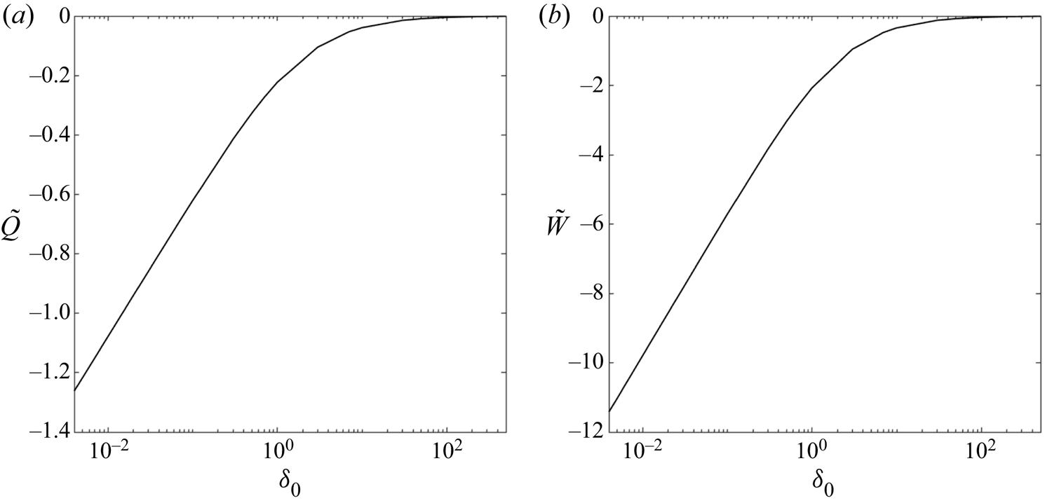
Figure 8 shows the behaviour of  $\tilde {W}(\delta _0)$ and
 $\tilde {Q}(\delta _0)$ as a function of
 $\delta _0$. This behaviour can be well approximated by the following fitted functions
 \begin{equation} \tilde Q = \frac{b_1+b_2 \ln\left(\dfrac{1}{\delta_0}+b_3\right)}{1+b_4\delta_0} , \end{equation}
where  $b_1 = -0.1580, b_2 = -1/5, b_3=0.65632, b_4 = 0.16330$ and
 \begin{equation} \tilde{W} = \frac{b_5+b_6 \ln\left(\dfrac{1}{\delta_0}+b_7\right)}{1+b_8\delta_0} , \end{equation}
where  $b_5 = -1.6448, b_6 = -\sqrt {\rm \pi}, b_7=0.59098, b_8 = 0.19167$. The relative error is less than
 $2\,\%$ over the entire range.
Graph of generalized pressure force function  $\tilde Q$ (a) and stress function
 $\tilde W$ (b) as functions of
 $\delta _0$ to describe the tangential resistivities for any size ratio and at any gap separation.

Applying this procedure to all the expressions in (3.34) and (3.35) yields
 \begin{gather} \left. \begin{gathered} \Delta f^{{\perp}}_{t,S} ={-} \Delta f^{{\perp}}_{t,P} = \tfrac{1}{3\sqrt{\rm \pi}}\tilde W + (2\alpha - 1)^{2} \tilde Q ,\\ \Delta f^{{\perp}}_{r,S} ={-}\Delta f^{{\perp}}_{r,P} ={-}\tfrac{1}{3\sqrt{\rm \pi}}\tilde W + (2\alpha - 1) \tilde Q , \end{gathered} \right\} \end{gather}
 \begin{gather} \left. \begin{gathered} \Delta t^{{\perp}}_{t,S} ={-} \tfrac{1}{4\sqrt{\rm \pi}}\tilde W + \tfrac{3}{4} (2\alpha - 1) \tilde Q ,\\ \Delta t^{{\perp}}_{t,P} ={-} \tfrac{1}{4\sqrt{\rm \pi}}\tilde W - \tfrac{3}{4} (2\alpha - 1) \tilde Q ,\\ \Delta t^{{\perp}}_{r,S} = \tfrac{1}{4\sqrt{\rm \pi}}\tilde W + \tfrac{3}{4} \tilde Q ,\\ \Delta t^{{\perp}}_{r,P} = \tfrac{1}{4\sqrt{\rm \pi}}\tilde W - \tfrac{3}{4} \tilde Q . \end{gathered} \right\} \end{gather}
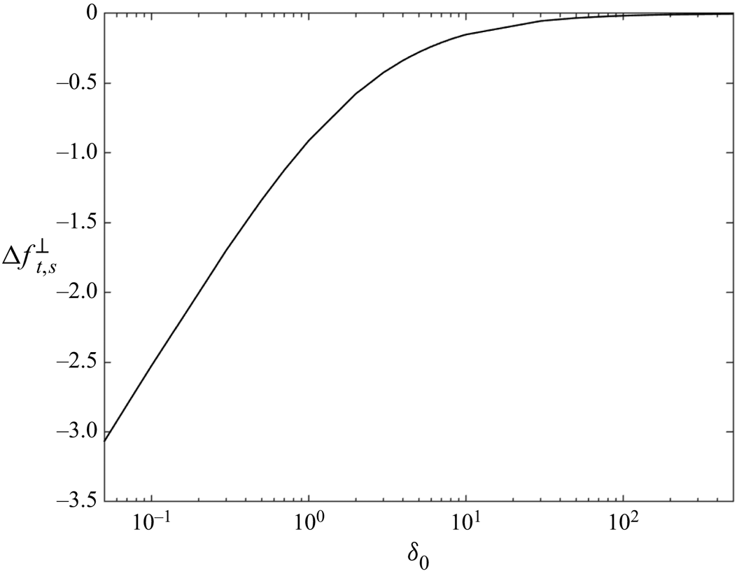
Figure 9 shows  $\Delta f_{t,S}^{\perp }$ as a function of
 $\delta _0$. Notice that the function approaches zero for large
 $\delta _0$ since the non-continuum inner solution approaches the continuum inner solution in that limit. Jeffrey & Onishi (Reference Jeffrey and Onishi1984) derived generalized expressions, and developed FORTRAN codes, for the continuum resistivities that smoothly transition from twin multipole expansions at large separations (O'Neill & Majumdar Reference O'Neill and Majumdar1970) to the matched asymptotic solutions in the lubrication regime shown in (3.46). These expressions can be extended to incorporate non-continuum lubrication flows, for
 $Kn\ll 1$, yielding uniformly valid resistivity functions, valid for arbitrary
 $\varepsilon$, as follows
 \begin{equation} \left. \begin{gathered} f^{{\perp}{UV}}_{t,S} = f^{{\perp}{JO}}_{t,S}(\varepsilon,\alpha) + \Delta f^{{\perp}}_{t,S}(\delta_0,\alpha) , \\ f^{{\perp}{UV}}_{t,P} = f^{{\perp}{JO}}_{t,P}(\varepsilon,\alpha) + \Delta f^{{\perp}}_{t,P}(\delta_0,\alpha) ,\\ f^{{\perp}{UV}}_{r,S} = f^{{\perp}{JO}}_{r,S}(\varepsilon,\alpha) + \Delta f^{{\perp}}_{r,S}(\delta_0,\alpha) , \\ f^{{\perp}{UV}}_{r,P} = f^{{\perp}{JO}}_{r,P}(\varepsilon,\alpha) + \Delta f^{{\perp}}_{r,P}(\delta_0,\alpha) , \\ t^{{\perp}{UV}}_{t,S} = t^{{\perp}{JO}}_{t,S}(\varepsilon,\alpha) + \Delta t^{{\perp}}_{t,S}(\delta_0,\alpha) , \\ t^{{\perp}{UV}}_{t,P} = t^{{\perp}{JO}}_{t,P}(\varepsilon,\alpha) + \Delta t^{{\perp}}_{t,P}(\delta_0,\alpha) ,\\ t^{{\perp}{UV}}_{r,S} = t^{{\perp}{JO}}_{r,S}(\varepsilon,\alpha) + \Delta t^{{\perp}}_{r,S}(\delta_0,\alpha) ,\\ t^{{\perp}{UV}}_{r,P} = t^{{\perp}{JO}}_{r,P}(\varepsilon,\alpha) + \Delta t^{{\perp}}_{r,P}(\delta_0,\alpha), \end{gathered} \right\} \end{equation}
where the superscript ‘ $JO$’ refers to the generalized resistivity functions taken from Jeffrey & Onishi (Reference Jeffrey and Onishi1984). Further details on the three-dimensional formulation of these equations are provided in Appendix A.
Example of  $\Delta f^{\perp }_t = \hat {f}^{NC}_t - \hat {f}^{C}_t$ obtained from (3.50) for
 $\alpha =1$. Non-continuum effects, corresponding to
 $\Delta f^{\perp }_t < 0$, are readily apparent for small
 $\delta _0$, whereas the function approaches zero in the continuum limit, corresponding to
 $\delta _0\gg 1$.

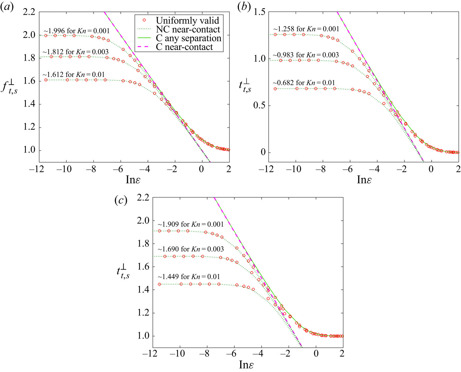
Figure 10 shows  $f^{\perp }_{t,S}$,
 $t^{\perp }_{t,S}$ and
 $t^{\perp }_{r,S}$ computed in various ways vs
 $\varepsilon$ at the indicated Knudsen numbers. In the large
 $\varepsilon$ limit, all three solutions approach the continuum solution,
 $f^{C}_{t}$ (solid line). The open circles were computed from (3.59) using (3.57), (3.58) and the curve fits for
 $\tilde Q$ and
 $\tilde W$ given in (3.55) and (3.56). The dotted green line shows the non-continuum lubrication approximation (3.49), which is valid in the limit of small
 $\varepsilon$ where the overall resistivity is dominated by the non-continuum inner resistivity. In this limit, each resistivity can be shown analytically to approach a constant. In the limit as
 $\delta _0 \rightarrow 0$, (3.55) and (3.56) reduce to
 \begin{equation} \left. \begin{gathered} \tilde Q \rightarrow b_1+b_2 \ln\left(\frac{1}{\delta_0}\right),\\ \tilde W \rightarrow b_5+b_6 \ln\left(\frac{1}{\delta_0}\right), \end{gathered} \right\} \end{equation}
which when substituted into (3.59) yields the asymptote as a function of  $Kn$
 \begin{align} \left. \begin{gathered} f^{{\perp}{UV}}_{t,S} \rightarrow \left[ -\frac{4}{15} \alpha(3 \alpha^{2}-3\alpha +2) \right] \ln\left(Kn\right) + \alpha \left[ b_1(2\alpha-1)^{2} +\frac{b_5}{3\sqrt{\rm \pi}} \right]+ A^{Y}_{22}(\alpha),\\ t^{{\perp}{UV}}_{t,S} \rightarrow \left[ \frac{1}{5} \alpha(3 \alpha -4) \right] \ln\left(Kn\right) - 2\alpha \left[ \frac{3}{4}b_1(2\alpha-1) - \frac{b_5}{4\sqrt{\rm \pi}} \right]+ B^{Y}_{22}(\alpha),\\ t^{{\perp}{UV}}_{r,S} \rightarrow \left[ -\frac{2}{5} \alpha \right] \ln\left(Kn\right) + \alpha \left[ \frac{3}{4}b_1 +\frac{b_5}{4\sqrt{\rm \pi}} \right]+ C^{Y}_{22}(\alpha), \end{gathered} \right\} \end{align}
where  $A^{Y}_{22}(0.5) = 0.9983$,
 $B^{Y}_{22}(0.5) = -0.2390$ and
 $C^{Y}_{22}(0.5) = 0.7028$ are the values for the
 $O(1)$ terms, respectively, for
 $\alpha = 0.5$ (Jeffrey & Onishi Reference Jeffrey and Onishi1984). There are only a few tabulated values provided in Jeffrey & Onishi (Reference Jeffrey and Onishi1984) so we modified their FORTRAN code to output the
 $O(1)$ terms for any size ratio. Figure 10 shows the asymptotic values of the resistivities in the limit as
 $\varepsilon \rightarrow 0$ for the different Knudsen numbers that were calculated.
The force on sphere  $S$ due to translation (a),
 $f^{\perp }_{t,S}$, torque due to translation (b),
 $t^{\perp }_{t,S}$, and torque due to rotation (c),
 $t^{\perp }_{r,S}$, is plotted as a function of
 $\varepsilon$ for Knudsen numbers 0.01, 0.003 and 0.001 and
 $\alpha = 0.5$. The open circles use (3.59), the dotted green line uses (3.49), the solid green line shows the generalized expression from Jeffrey & Onishi (Reference Jeffrey and Onishi1984) and the magenta dashed line is using (3.46).

It is well known that the tangential force due to particle rotation and the torque due to tangential relative translation satisfy the reciprocal relation
 \begin{equation} \frac{f^{{\perp}{JO}}_{r,S}}{t^{{\perp}{JO}}_{t,S}} = \frac{4}{3} . \end{equation}
This equation was derived by Lorentz (Reference Lorentz1896) using the reciprocal theorem for the continuum Stokes flow equations and a no-slip boundary condition. However, a derivation based on Onsager's reciprocal relations (Onsager Reference Onsager1931a,Reference Onsagerb) for near equilibrium fluids can be used to show that the same relation holds for particles in any fluid exhibiting a linear response due to a small deviation from equilibrium (Landau & Lifshitz Reference Landau and Lifshitz1980; Ying & Peters Reference Ying and Peters1989; Zhang, Xu & Qian Reference Zhang, Xu and Qian2015) including a non-continuum gas governed by the linearized Boltzmann equation and a gas described using the Stokes equations with a Maxwell slip boundary condition. Consistent with this expectation, we can see from (3.57) and (3.58) that
 \begin{equation} \frac{\Delta f^{{\perp}}_{r,S}}{\Delta t^{{\perp}}_{t,S}} = \frac{4}{3} , \end{equation}
implying
 \begin{equation} \frac{f^{{\perp}{UV}}_{r,S}}{t^{{\perp}{UV}}_{t,S}} = \frac{4}{3} \end{equation}
at all separations.
4. Sphere settling adjacent to a vertical wall
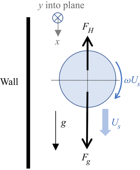
The canonical problem of a sphere settling adjacent to a vertical wall in an otherwise quiescent, semi-infinite fluid is considered by setting  $\alpha = 1$. At steady state, the sphere is assumed to have a translational velocity
 $U_S$ and a rotation rate
 $a_S \varOmega$, as illustrated in figure 11. The steady state results from a force and torque balance. Introducing the resistance functions derived earlier we have
 \begin{equation} F_H \equiv{-} 6{\rm \pi}\mu a (U_S f_{t, S}^{{\perp}{UV}} +a_S \varOmega f_{r, S}^{{\perp}{UV}}), \end{equation}
such that the resulting force balance in the  ${x}$-direction is
 \begin{equation} F_{x} = F_g + F_H = 0 , \end{equation}
where  $F_g = mg$ is the force due to gravity. In the absence of external torques, the resultant torque acting on the particle in the
 $y$-direction is
 \begin{equation} T_{y} ={-} 8{\rm \pi} \mu a a_S \left(U_S t_{t, S}^{{\perp}{UV}}+ a_S \varOmega t_{r,S}^{{\perp}{UV}}\right)=0 . \end{equation}
Notice that only the tangential resistivities are involved in this motion. From equations (4.1) and (4.3), the force balance becomes
 \begin{equation} 6{\rm \pi}\mu a U_S\left[f_{t, S}^{{\perp}{UV}} + \omega f_{r, S}^{{\perp}{UV}}\right] = mg, \end{equation}
where  $\omega$ is determined by
 \begin{equation} \omega ={-}\frac{t_{t, S}^{{\perp}{UV}}}{t_{r, S}^{{\perp}{UV}}}. \end{equation}
Sketch of a particle settling vertically with a wall at steady state where hydrodynamic  $F_H$ forces are balanced by gravitational force
 $F_g$.

We analyse the motion of spheres with Knudsen numbers 0.01, 0.001 and 0.0001. We solve (4.5) for  $\omega$ and substitute that into (4.4) to obtain
 $U_S$. Figure 12(a) shows the normalized settling velocity
 $U_S/U^{(0)}$, where
 $U^{(0)}$ is the terminal velocity in an unbounded fluid and
 $\varepsilon = h_0/a$, and (b) shows the rotation rate
 $\omega$ as a function of
 $\varepsilon$.
Graph of non-continuum settling velocity normalized by the settling velocity of the isolated particle (a) and ratio of angular to translational velocities  $\omega$ (b) at different
 $\varepsilon$ for spheres with Knudsen numbers of 0.01, 0.001 and 0.0001.

Goldman, Cox & Brenner (Reference Goldman, Cox and Brenner1967) analysed a sphere in a continuum fluid settling under gravity adjacent to a vertical plane and argued that a no-slip condition would require  $\omega = 1$, and since their continuum results indicated an asymptotic value of 0.25 in the limit as
 $\varepsilon \to 0$, the sphere has to roll and slip. Our non-continuum results show even lower asymptotic values of
 $\omega$, suggesting even greater slipping is occurring than for the continuum case. To our knowledge, no experimental measurements exist in this regime.
A second observation pertains to the discrepancy between the continuum and non-continuum settling velocities in the limit as the gap goes to zero. The continuum approximation predicts the velocity vanishes in this limit, or equivalently the sphere will ‘stick’ to the wall due to the diverging hydrodynamic force. Figure 12(a) shows that the non-continuum theory predicts a constant settling velocity as the gap goes to zero. The experiment by Carty (Reference Carty1957) yielded a terminal speed for a sphere near a wall that was constant for small gap separations, consistent with the prediction of the non-continuum theory; however, Goldman et al. (Reference Goldman, Cox and Brenner1967) noted their results were also consistent with solid-body friction caused by surface roughness, underscoring the need for experiments in which the effects due to roughness have been carefully eliminated.
5. Conclusions
In this paper, we have derived uniformly valid resistivity functions for the forces and torques between two unequal size spheres moving or rotating through a gas in a direction perpendicular to their line of centres at low Reynolds and Mach numbers. The expressions were derived using a matched asymptotic analysis taking into consideration the non-continuum flow that occurs between the spheres when their minimum separation distance is comparable to or smaller than the mean free path of the gas. The analysis assumes the Knudsen number is small such that the non-continuum flow is restricted to the inner lubrication region. The lubrication flow was expressed as a superposition of its three constituent flows: Poiseuille flow, Couette flow and plug flow. The relative weights of the three flows were determined by the boundary conditions and by the pressure field. To account for the non-continuum flow in the gap, we applied the solutions for Poiseuille flow and Couette flow found by Cercignani & Pagani (Reference Cercignani and Pagani1966), who solved the BGK approximation to the linearized Boltzmann equation. Substituting these expressions into the lubrication approximation for the flow in the gap yielded the differential equation describing the pressure and the stress that then could be integrated over the surface of the sphere to obtain the non-continuum ‘inner’ solution for the force and torque acting on the sphere. As we are interested in spheres with asymptotically small Knudsen numbers, the outer flow is always in the continuum regime regardless of the gap separation. A non-continuum correction to the inner solution was obtained by subtracting the inner solution for the continuum fluid from the inner solution for the non-continuum fluid and curve fitting the result. Adding to that the generalized resistivity functions for a continuum fluid derived by Jeffrey & Onishi (Reference Jeffrey and Onishi1984) yielded uniformly valid expressions for the four tangential resistivity functions that smoothly transition from the continuum expressions for  $\delta _0\gg 1$ to the free molecular expressions for
 $\delta _0\ll 1$.
For spheres nearly in contact, the continuum tangential resistivities diverge logarithmically with decreasing gap separation. However, in the pseudo-free molecular regime, the non-continuum lubrication flow yields resistivities that asymptote to a constant that scales like  $\ln (Kn^{-1})$. We apply the resulting expressions to the case of a sphere settling adjacent to a vertical wall. At separations large in comparison to the mean free path of the gas, the sphere settles and rotates at rates that correspond to the continuum solution. As the minimum gap separation approaches and goes below the mean free path of the gas, the settling speed and rotation rate are modified by the non-continuum flow; the settling speed is increased and the dimensionless rotation rate,
 $a_S\varOmega /U_S$, is decreased, but
 $a_S\varOmega$ is increased relative to the continuum fluid. For a sphere in contact with the wall, the continuum solution predicts the velocity and rotation of the sphere vanish causing the sphere to ‘stick’ to the wall due to hydrodynamic resistance only, whereas the non-continuum resistivities yield a finite settling and rotation speed at contact, consistent with experiments (Carty Reference Carty1957).
A primary motivation for this study is to resolve the near-contact motion of cloud droplets in the atmosphere. The continuum lubrication flow generates a normal force that diverges like  $\varepsilon ^{-1}$ and a tangential force that diverges like
 $\ln (\varepsilon ^{-1})$. As a consequence, two cloud droplets on a colliding trajectory would not be able to come into physical contact, as the resistive force would stop their relative motion. This would imply that cloud droplets could only grow by condensation. The results developed here, along with the earlier work of Sundararajakumar & Koch (Reference Sundararajakumar and Koch1996), provide a complete explanation for coalescence in the Stokes regime, namely the weaker lubrication forces that result from the non-continuum lubrication flow between the droplets at gap separations below the mean free path of the gas allow coalescence to occur in finite time. Thus, the resistance functions developed in this paper play a critical role in understanding the evolution of atmospheric clouds.
Acknowledgements
This study was supported by the National Science Foundation grant number CBET 1605195. The authors gratefully acknowledge the National Center for Atmospheric Research (NCAR) for providing high performance computing resources on Cheyenne.
Declaration of interests
The authors report no conflict of interest.
Appendix A. Vector formulation of the non-continuum resistivity tensor
This appendix presents the vector formulation for the resistivity tensor for two particles moving through a quiescent fluid. We begin with the continuum formulation of Jeffrey & Onishi (Reference Jeffrey and Onishi1984), and incorporate the uniformly valid tangential expressions developed herein and the uniformly valid expressions derived by Sundararajakumar & Koch (Reference Sundararajakumar and Koch1996) for the normal force. It should be noted that the scaling used by Jeffrey & Onishi (Reference Jeffrey and Onishi1984) to non-dimensionalize the equations differs from ours. They used the arithmetic mean radius for their length scale and introduced a size ratio,  $\kappa$, defined as
 \begin{equation} \kappa = \frac{a_2}{a_1} , \end{equation}
which is related to  $\alpha$ by
 \begin{equation} \alpha = \frac{1}{1+\kappa} . \end{equation}
Throughout the appendix, we have adapted the expressions derived in this paper to their basis to simplify the evaluation of the uniformly valid expressions. Furthermore, we replace the labels ‘ $P$’ and ‘
 $S$’ with ‘1’ and ‘2’ to facilitate writing the tensor relationships. The analysis in the appendix allows both spheres to move – the motion of each sphere induces a force and torque on each sphere, giving rise to four separate interactions. We introduce the subscripts ‘
 $\gamma \sigma$’ to represent the force (or torque) acting on sphere
 $\gamma$ due to the motion of sphere
 $\sigma$, where
 $\gamma$ and
 $\sigma$ can each be either 1 or 2. We extend the expressions derived in the paper to the general case.
The equation for the force and torque acting on particles 1 and 2 can be written as (Jeffrey & Onishi Reference Jeffrey and Onishi1984)
 \begin{equation} \begin{pmatrix}
\boldsymbol{F}_1\\ \boldsymbol{F}_2\\ \boldsymbol{T}_1\\
\boldsymbol{T}_2\end{pmatrix} = \begin{pmatrix}
\boldsymbol{\mathsf{A}}_{11} & \boldsymbol{\mathsf{A}}_{12} &
\tilde{\boldsymbol{\mathsf{B}}}_{11} & \tilde{\boldsymbol{\mathsf{B}}}_{12}\\
\boldsymbol{\mathsf{A}}_{21} & \boldsymbol{\mathsf{A}}_{22} &
\tilde{\boldsymbol{\mathsf{B}}}_{21} & \tilde{\boldsymbol{\mathsf{B}}}_{22}\\
\boldsymbol{\mathsf{B}}_{11} & \boldsymbol{\mathsf{B}}_{12} &
\boldsymbol{\mathsf{C}}_{11} & \boldsymbol{\mathsf{C}}_{12}\\
\boldsymbol{\mathsf{B}}_{21} & \boldsymbol{\mathsf{B}}_{22} &
\boldsymbol{\mathsf{C}}_{21} & \boldsymbol{\mathsf{C}}_{22}\\ \end{pmatrix}
\begin{pmatrix} \boldsymbol{U}_1\\ \boldsymbol{U}_2\\
\boldsymbol{\varOmega}_1\\ \boldsymbol{\varOmega}_2\\
\end{pmatrix} \end{equation}
where  $\boldsymbol {F}_1$,
 $\boldsymbol {F}_2$,
 $\boldsymbol {T}_1$ and
 $\boldsymbol {T}_2$ are the forces and torques acting on particles 1 and 2,
 $\boldsymbol{\mathsf{A}}$,
 $\boldsymbol{\mathsf{B}}$,
 $\tilde {\boldsymbol{\mathsf{B}}}$ and
 $\boldsymbol{\mathsf{C}}$ are second rank tensors (defined below) and
 $\boldsymbol {U}_1$,
 $\boldsymbol {U}_2$,
 $\boldsymbol {\varOmega }_1$ and
 $\boldsymbol {\varOmega }_2$ are the translational and rotational velocities for particles 1 and 2. We define the separation vector,
 $\boldsymbol {r}\equiv \boldsymbol {x}_2 - \boldsymbol {x}_1$, where
 $\boldsymbol {x}_1$ and
 $\boldsymbol {x}_2$ are the positions of the centres of particles 1 and 2, respectively. The unit vector along the line of centres is
 $\hat {\boldsymbol {r}}\equiv \boldsymbol {r}/|\boldsymbol {r}|$. The minimum gap separation between the particles is then
 $h_0 = |\boldsymbol {r}| - (a_1 + a_2)$, and we retain the definitions of
 $\varepsilon$ and
 $\delta _0$ from the main paper.
It is convenient to introduce index notation such that  $A_{ij}^{\gamma \sigma } = \boldsymbol{\mathsf{A}}_{\gamma \sigma }$, where indices
 $i$ and
 $j$ indicate directions and
 $\gamma$ and
 $\sigma$ are either 1 or 2. For example,
 $\boldsymbol{\mathsf{A}}_{12} = {\mathsf{A}}_{ij}^{12}$. The tensors in (A3) are then given in dimensional form consistent with the notations of Jeffrey & Onishi (Reference Jeffrey and Onishi1984) (note the difference with the (3.32a,b) and (3.33a,b) in the main paper)
 \begin{gather} {\mathsf{A}}_{ij}^{\gamma\sigma} ={-}6{\rm \pi}\mu\left(\frac{a_\gamma+ a_\sigma}{2}\right)[f^{{\parallel}{UV}}_{t,\gamma\sigma} \hat{r}_i\hat{r}_j + f^{{\perp}{UV}}_{t,\gamma\sigma}(\delta_{ij} - \hat{r}_i\hat{r}_j)] , \end{gather}
 \begin{gather} {\mathsf{B}}_{ij}^{\gamma\sigma} ={-}4{\rm \pi}\mu\left(\frac{a_\gamma+ a_\sigma}{2}\right)^{2} t_{t,\gamma\sigma}^{{\perp}{UV}}\epsilon_{ijk}\hat{r}_k , \end{gather}
 \begin{gather} \tilde{{\mathsf{B}}}_{ij}^{\gamma\sigma} ={-}4{\rm \pi}\mu\left(\frac{a_\gamma+ a_\sigma}{2}\right)^{2} t_{t,\sigma\gamma}^{{\perp}{UV}}\epsilon_{jik}\hat{r}_k , \end{gather}
 \begin{gather} {\mathsf{C}}_{ij}^{\gamma\sigma} ={-}8{\rm \pi}\mu\left(\frac{a_\gamma+ a_\sigma}{2}\right)^{3} [t^{{\parallel}{JO}}_{r,\gamma\sigma} \hat{r}_i\hat{r}_j + t^{{\perp}{UV}}_{r,\gamma\sigma}(\delta_{ij} - \hat{r}_i\hat{r}_j)] , \end{gather}
where  $\hat {r}_i$ is the unit normal vector pointing from particle 1 to particle 2,
 $\delta _{ij}$ is the Kronecker delta function and
 $\epsilon _{ijk}$ is the alternating unit tensor. The scalar resistivity functions are defined as
 \begin{gather} f^{{\perp}{UV}}_{t,\gamma \sigma} = Y^{{A}}_{\gamma\sigma}(\varepsilon,\kappa) + ({-}1)^{(\gamma+\sigma)} a_{\gamma\sigma} \left[\frac{1}{3 \sqrt{\rm \pi}}\tilde{W}(\delta_0) + \left(\frac{1-\kappa}{1+\kappa}\right)^{2} \tilde{Q}(\delta_0)\right] , \end{gather}
 \begin{gather}t^{{\perp}{UV}}_{t,\gamma\sigma} = Y^{{B}}_{\gamma\sigma}(\varepsilon,\kappa) + 2 a_{\gamma\sigma}\left(\frac{a_\gamma}{a_m}\right)^{|\gamma-\sigma|} \left[\frac{({-}1)^{\sigma}}{4\sqrt{\rm \pi}} \tilde{W}(\delta_0) - ({-}1)^{(\gamma+\sigma)} \frac{3}{4}\left(\frac{1-\kappa}{1+\kappa}\right) \tilde{Q}(\delta_0)\right] , \end{gather}
 \begin{gather}t^{{\perp}{UV}}_{r,\gamma\sigma} = Y^{{C}}_{\gamma\sigma}(\varepsilon,\kappa) + a_{\gamma\sigma}\left(\frac{2a}{a_m}\right)^{|\gamma-\sigma|} \left[\frac{1}{4 \sqrt {\rm \pi}}\tilde{W}(\delta_0) + ({-}1)^{(\gamma+\sigma)} \frac{3}{4}\tilde{Q}(\delta_0)\right], \end{gather}
where  $a_m\equiv (a_1+a_2)/2$ is the arithmetic mean radius,
 \begin{equation} a_{\gamma\sigma}\equiv a \left(\frac{a_\gamma + a_\sigma}{2}\right)^{{-}1} , \end{equation}
and  $Y^{{A}}_{\gamma \sigma }$,
 $Y^{{B}}_{\gamma \sigma }$ and
 $Y^{{C}}_{\gamma \sigma }$ are the tangential resistivities defined in Jeffrey & Onishi (Reference Jeffrey and Onishi1984).
The normal resistivity,  $f^{\parallel {UV}}_{t,\gamma \sigma }$ is given by
 \begin{equation} f^{{\parallel}{UV}}_{t,\gamma\sigma} = X^{{A}}_{\gamma\sigma}(\epsilon,\kappa) + ({-}1)^{(\gamma+\sigma)} a_{\gamma\sigma} \left(\frac{f^{{\parallel}}_{{fit}}(\delta_0,\kappa)}{Kn} - \frac{1}{\varepsilon}\right) , \end{equation}
where  $X^{{A}}_{\gamma \sigma }$ is the continuum resistivity (Jeffrey & Onishi Reference Jeffrey and Onishi1984) and
 $f^{\parallel }_{{fit}}$ can be expressed as (Sundararajakumar & Koch Reference Sundararajakumar and Koch1996)
 \begin{equation} f^{{\parallel}}_{{fit}}= \left\{ \begin{array}{@{}ll} \displaystyle \dfrac{\rm \pi}{6} \left( \ln t - \dfrac{1}{t} - \dfrac{1}{t^{2}} - \dfrac{2}{t^{3}} \right)\\ \displaystyle \quad\quad + 1.5475\delta_0^{2} +0.7896\delta_0+0.4094 & (\delta_0<0.35)\\ \displaystyle 0.00006 \left( \dfrac{1}{\delta_0} \right)^{3} - 0.00172 \left(\dfrac{1}{\delta_0} \right)^{2}+0.0169\left(\dfrac{1}{\delta_0} \right)\\ \displaystyle \quad\quad 0.1769 \ln \left(\dfrac{1}{\delta_0} \right) +0.3744 & (0.35<\delta_0<0.9)\\ \displaystyle 0.00050\delta_0^{4}-0.00835\delta_0^{3}+0.05605\delta_0^{2}-0.2196\delta_0 +0.5661\\ \displaystyle \quad-0.0055\left(\dfrac{1}{\delta_0} \right)-0.01965\left(\dfrac{1}{\delta_0} \right)^{2}+0.0231\left(\dfrac{1}{\delta_0} \right)^{3} & (0.9<\delta_0<4.4)\\ \displaystyle \dfrac{1}{18k_1^{2}} \left[ (6k_1+\delta_0)\ln \left( 1+\dfrac{6k_1}{\delta_0} \right) - 6k_1 \right] & (\delta_0>4.4) \end{array} \right. \end{equation}
and  $t = \ln (1/\delta _0) + 0.8$. We note that the coefficients in (A13) differ from those in Sundararajakumar & Koch (Reference Sundararajakumar and Koch1996) because we did not apply the correction factor
 $\sqrt {{\rm \pi} }/2$ to the mean free path from the BGK theory to make it consistent with that for a hard sphere gas, as they did. While that correction factor can be easily incorporated into the normal resistivity, for which the pressure equation can be integrated analytically, the same correction applied to the tangential resistivities introduces a discontinuity into the equation for the pressure field that precludes its numerical integration. Consequently, we use the BGK mean free path throughout for consistency. Finally, we note that there is no non-continuum flow generated by the torque acting in the normal direction,
 $t^{\parallel {JO}}_{r,\gamma \sigma } \equiv X^{{C}}_{\gamma \sigma }$, and hence we apply the Jeffrey & Onishi (Reference Jeffrey and Onishi1984) expression directly.
We make available an open source code that computes the above equations.