1. Introduction
Parametric resonance is a phenomenon that generates a large periodic response in a single-degree-of-freedom system as a result of periodic modulation of the system’s natural frequency. Unless the system is non-dissipative and the frequency of excitation is precisely equal to the natural frequency, resonance occurs only when the amplitude of excitation surpasses a critical threshold. Normally, the lowest threshold produces a response whose frequency is exactly half that of the parametric frequency. This excitation, known as subharmonic parametric resonance, is the foundation for a wide range of physical phenomena. Early examples include the string vibration experiments conducted by Melde (Reference Melde1860) and Raman (Reference Raman1912) and the model of the lunar perigee by Hill (Reference Hill1886). Most generally, this resonance is described by the Mathieu equation, which Ruby (Reference Ruby1996) has shown to model a variety of systems in which periodic gravitational, electric and magnetic fields are used to drive the resonant response. In modern practical applications, Turner et al. (Reference Turner, Miller, Hartwell, MacDonald, Strogatz and Adams1998) have investigated parametric resonance in microelectromechanical systems (MEMS) and Prakash et al. (Reference Prakash, Hu, Raman and Reifenberger2009) have considered applications to atomic force microscopy.
Faraday waves may be the most well-known example of parametric resonance in fluid systems. The waves, first reported by Faraday (Reference Faraday1831), arise from an instability where standing wave patterns grow at a fluid interface when a periodic vertical motion of
 $A\text{cos}{\it\omega}t$
is imposed onto the holding container. For a container with sufficiently large lateral dimensions, the wavelength increases monotonically with vibrational frequency, and the generated pattern is independent of the container geometry. This regime has garnered significant experimental and theoretical attention owing to the relative ease with which a rich variety of patterns can be generated. Two-frequency excitations are commonly used in this regime as a means to break temporal symmetries and realize patterns unavailable to single-frequency excitation (Müller Reference Müller1993; Edwards & Fauve Reference Edwards and Fauve1994; Kudrolli & Gollub Reference Kudrolli and Gollub1996; Arbell & Fineberg Reference Arbell and Fineberg2002). The single-frequency (Kumar & Tuckerman Reference Kumar and Tuckerman1994) and two-frequency (Besson, Edwards & Tuckerman Reference Besson, Edwards and Tuckerman1996) linear theories for horizontally infinite immiscible viscous bilayers give excellent prediction of the experimental threshold
 $A$
at which a wavenumber
 $k$
is excited, by both experiment (Bechhoefer et al.
Reference Bechhoefer, Ego, Manneville and Johnson1995; Besson et al.
Reference Besson, Edwards and Tuckerman1996) and direct numerical simulation (Perinet, Juric & Tuckerman Reference Perinet, Juric and Tuckerman2009). Furthermore, single- and two-frequency nonlinear theories have been developed to capture features of the pattern formation processes (Milner Reference Milner1991; Zhang & Viñals Reference Zhang and Viñals1997a
; Skeldon & Guidoboni Reference Skeldon and Guidoboni2007).
Relative to the pattern-forming qualities of the high-frequency excitation, less attention has been given to single-mode Faraday waves, which is the name given by Henderson & Miles (Reference Henderson and Miles1990) to the regime in which the lateral dimensions of the container are small. In contrast to the laterally infinite regime, the spatial form of the wave in a small container is strongly influenced by its lateral geometry and the sidewall behaviour of the fluid interface. These conditions effectively discretize the wavenumbers allowed by the system, in the same manner in which energy levels are discretized in a quantum system. As a result, the monotonic dependence of the wavenumber on the excitation frequency is lost, and, instead, a single wavenumber is excited for a band of frequencies. Compared to the laterally infinite regime, the nonlinear response is far greater for single-mode excitation, and therefore a promising application is mixing in microfluidic systems. Notably, Xu & Attinger (Reference Xu and Attinger2007) generated single-mode Faraday waves on a
 $100~{\rm\mu}\text{m}$
air–water interface using ultrasonic acoustic actuation. Agrawal, Gandhi & Neild (Reference Agrawal, Gandhi and Neild2014) have investigated particle collection at the antinodes of single-mode Faraday waves in small (
 $4~\text{mm}\times 5~\text{mm}\times 0.25~\text{mm}$
) containers. Also, Harris et al. (Reference Harris, Moukhtar, Fort, Couder and Bush2013) have shown that the path statistics of a walking droplet directly correlate to the spatial form of a single-mode Faraday wave in a small cylindrical system.
A major challenge of single-mode Faraday waves is the prediction of the frequency bands and critical amplitudes of instability in an experiment. It is notoriously difficult to model the dissipation of surface waves when sidewall effects such as Stokes boundary layers and dynamic contact angles are significant (Miles Reference Miles1967; Hocking Reference Hocking1987), which has led previous single-mode works to model these effects phenomenologically via linear damping. Although satisfactory agreement has been seen when this parameter is measured from the experimental wave decay (Henderson & Miles Reference Henderson and Miles1990; Tipton & Mullin Reference Tipton and Mullin2004; Das & Hopfinger Reference Das and Hopfinger2008), a major drawback is that this parameter must be measured for each cell mode to determine global stability. An alternative approach was taken by the recent work of the authors (Batson, Zoueshtiagh & Narayanan Reference Batson, Zoueshtiagh and Narayanan2013), who developed an experiment in a cylindrical container with the aim to minimize sidewall effects. By judicious choice of fluids and sidewall materials, the overall system dissipation was controlled by the bulk-phase viscous effects, and remarkable agreement with the linear theory of Kumar & Tuckerman (Reference Kumar and Tuckerman1994) was found for a wide range of cell modes when the stress-free boundary condition was applied to effect mode discretization.
The focus of this paper is to use the experiment of Batson et al. (Reference Batson, Zoueshtiagh and Narayanan2013) to conduct the first known study of single-mode Faraday waves excited with two parametric frequencies. Consideration of a second frequency is of fundamental relevance to space operations, where the well-known effect of
 $g$
-jitter leads to a wide range of vibrational frequencies (Monti & Savino Reference Monti and Savino1996). Our main effort therefore is to characterize the influence of a second frequency on the linear threshold. We approach this theoretically for single-mode excitation by application of the stress-free condition to the linear theory of Besson et al. (Reference Besson, Edwards and Tuckerman1996). The model predicts that the onset of instability is affected most significantly when the added frequency is exactly twice the primary frequency, which we report experimentally for harmonic excitation of the fundamental axisymmetric mode. Moreover, we show that for this case the phase lag between the two frequencies is critically important, in accordance with this model and a theoretical result established by Zhang & Viñals (Reference Zhang and Viñals1997b
) for laterally large systems. Experiments are also presented for cases where the influence of a second frequency on the threshold is minimal. Overall, agreement between the model and the experiment is identical to that observed by Batson et al. (Reference Batson, Zoueshtiagh and Narayanan2013) for single-frequency excitation.
The secondary focus is to characterize the experimental nonlinear response to two-frequency excitation, as was done for single-frequency excitation by Henderson & Miles (Reference Henderson and Miles1990), Tipton & Mullin (Reference Tipton and Mullin2004) and Das & Hopfinger (Reference Das and Hopfinger2008). We demonstrate that, even for cases where the influence of the second frequency on the linear threshold is not noticeable, the nonlinear response may be altered significantly. Additionally, we present an example of a novel wave in which two spatial modes are simultaneously locked to the separate excitation frequencies. Similar two-mode waves in the single-frequency experiment of Ciliberto & Gollub (Reference Ciliberto and Gollub1985) were shown to exhibit quasi-periodic and chaotic dynamics. The nonlinear interactions of two modes excited by a single frequency were further studied experimentally (Simonelli & Gollub Reference Simonelli and Gollub1989; Henderson & Miles Reference Henderson and Miles1991) and theoretically (Meron & Procaccia Reference Meron and Procaccia1986; Umeki & Kambe Reference Umeki and Kambe1989; Crawford, Knobloch & Riecke Reference Crawford, Knobloch and Riecke1990). Finally, in the single-frequency experiments of Batson et al. (Reference Batson, Zoueshtiagh and Narayanan2013), it was observed that meniscus waves emanating from the container sidewall could lower the apparent instability threshold for harmonic modes. In this work we again draw attention to this response, and we offer additional insight into the context of two-frequency excitation in our concluding remarks.
The course of the paper is as follows. First, considerations for the design of a two-frequency investigation are presented in the context of the general equation for parametric resonance, the Mathieu equation, and the analytical form of the two-frequency excitation function. Then, we analyse these considerations in detail for the single-mode Faraday system using the linear theory of Besson et al. (Reference Besson, Edwards and Tuckerman1996), modified to account for stress-free sidewalls. Two-frequency experiments are notably more challenging than those presented in Batson et al. (Reference Batson, Zoueshtiagh and Narayanan2013), as addition of a second component requires Fourier analysis to characterize the parametric input. Thus, before presenting the experimental results, we provide detailed discussion of our methods and the potential influence of stray signal harmonics.
2. Parametric resonance and two-frequency excitation
To introduce fundamental aspects of the linear theory for Faraday waves, first consider the single-degree-of-freedom system
 $$\begin{eqnarray}\partial _{tt}u+[p+2qG(t)]u=0,\end{eqnarray}$$
where the function
 $G(t)=\text{cos}\,2t$
. The parameter
 $p$
represents a natural frequency of the system and
 $q$
the amplitude of the excitation function. This is the classical form of the Mathieu equation, whose solutions are covered by McLachlan (Reference McLachlan1947). A connection between Faraday waves and the Mathieu equation was first drawn by Benjamin & Ursell (Reference Benjamin and Ursell1954), who analysed the linear stability of a horizontally infinite inviscid fluid. In their model, the parameter
 $p$
represented the natural frequency of a wavenumber
 $k$
, accounting for the density of the fluid and the surface tension, and
 $q$
, the amplitude of gravitational modulation. Solutions of the differential equation (2.1) reveal regions in the
 $p{-}q$
parameter space where the solution
 $u$
decays or grows without bound in time. Transition from a decaying solution to a resonant unstable solution may be observed by sufficient increase in the parameter
 $q$
for fixed
 $p$
, hence parametric. The threshold at which this occurs corresponds to a neutral growth rate, and may be determined either using multiple-scale or harmonic balance methods (Nayfeh & Mook Reference Nayfeh and Mook1979).
In this work two-frequency excitation of the form
 $$\begin{eqnarray}G(t)=A[\text{cos}{\it\chi}\text{cos}(l{\it\omega}t)+\sin {\it\chi}\text{cos}(m{\it\omega}t+{\it\phi})]\end{eqnarray}$$
will be considered, where the mixing angle
 ${\it\chi}$
is used to divide the overall excitation amplitude
 $A$
between the two commensurate frequencies
 $l{\it\omega}$
and
 $m{\it\omega}$
. This form
 $G(t)$
was first considered in the pattern formation study of Edwards & Fauve (Reference Edwards and Fauve1993). Here
 $l$
and
 $m$
are integers,
 ${\it\omega}$
is the basic frequency and
 ${\it\phi}$
is the phase lag. It is worth noting that, while the behaviour of the Mathieu equation is largely indifferent to whether
 $G(t)$
is a cosine or a sine, this choice is not trivial for two-frequency excitation, as the definition of the phase lag
 ${\it\phi}$
changes, which depends upon
 $m/l$
. Angles of
 ${\it\chi}=0$
and 90° thus represent single-frequency excitation at
 $l{\it\omega}$
and
 $m{\it\omega}$
, respectively. Intermediate values represent the case of two-frequency excitation with component amplitudes
 $A\text{cos}{\it\chi}$
and
 $A\sin {\it\chi}$
.
It will be seen that the two frequencies independently determine the wavenumber selection of the discretized Faraday system. That is, the same wavenumber excited with a single frequency
 $l{\it\omega}$
continues to be excited when small amplitudes of a second
 $m{\it\omega}$
component are added to the signal. Throughout, we refer to the
 $l{\it\omega}$
component in this situation as the ‘primary’ component. While the
 $m{\it\omega}$
component does not alter the wavenumber, it may result in increase or decrease of the
 $l{\it\omega}$
component amplitude
 $A\text{cos}{\it\chi}$
at criticality. Therefore, a major purpose of this study is to characterize adjustment of the linear threshold with respect to the amplitude, frequency and phase of the second component.
The experimental plan is to consider unique excitations of the fundamental axisymmetric mode, as suggested by predictions of the linear analysis. First, we examine two excitations, one with a second frequency
 $m{\it\omega}$
larger than the primary
 $l{\it\omega}$
, and the other with smaller
 $m{\it\omega}$
. For both, the
 $m{\it\omega}$
component primarily excites a different wavenumber when its relative amplitude is sufficiently large. The range of
 ${\it\chi}$
is therefore separated into one band from
 ${\it\chi}=0^{\circ }$
to
 ${\it\chi}_{c}$
, inside of which the fundamental axisymmetric mode is primarily excited by the
 $l{\it\omega}$
component. In the upper band extending from
 ${\it\chi}={\it\chi}_{c}$
to 90°, the
 $m{\it\omega}$
wavenumber is excited. The onset behaviour for all
 ${\it\chi}$
is compared to the linear theory, and nonlinear behaviour is characterized for the fundamental axisymmetric mode. The intersection of the lower and upper
 ${\it\chi}$
bands is also of interest, because this critical
 ${\it\chi}_{c}$
marks a codimension-two point at which both the
 $l{\it\omega}$
and
 $m{\it\omega}$
wavenumbers are simultaneously unstable. We therefore present the nonlinear experimental behaviour of a two-mode wave near this point. Finally, we conclude by observing strong dependence of the experimental onset on the phase difference
 ${\it\phi}$
for simultaneous harmonic (
 ${\it\omega}$
) and subharmonic (
 $2{\it\omega}$
) excitation of the fundamental axisymmetric mode.
3. Linear theory
The linear theory for the Faraday instability of two immiscible viscous fluids of horizontally infinite span, subjected to two-frequency vibrations of the form (2.2), was given by Besson et al. (Reference Besson, Edwards and Tuckerman1996). This theory is a slight extension to the single-frequency theory of Kumar & Tuckerman (Reference Kumar and Tuckerman1994), which is reviewed in Batson et al. (Reference Batson, Zoueshtiagh and Narayanan2013). We therefore refer the reader who is interested in the manipulations of the hydrodynamic equations to these works, and here we review only the key elements of the theory.
The model consists of two horizontally unbounded fluids separated by an interface of tension
 ${\it\gamma}$
. These layers are characterized by their densities
 ${\it\rho}_{j}$
, kinematic viscosities
 ${\it\nu}_{j}$
and heights
 $h_{j}$
, where the index
 $j=1,2$
represents the lower and upper phases, respectively. The Navier–Stokes equations and continuity describe bulk-phase dynamics and are written in a reference frame that moves with the excitation. Continuity of the phase velocities is set at the position of the deformable interface
 $z=Z(\boldsymbol{x},t)$
, and it is here that the dynamics of the bulk phases are coupled to each other. The kinematic condition at
 $z=Z(\boldsymbol{x},t)$
equates the normal components of the fluid velocities to the interface motion, and the interfacial stress balance equates phase pressures and viscous stresses to those arising from surface curvature.
This nonlinear system has a trivial solution of zero flow and a flat interface, and its stability is analysed at linear order by considering infinitesimal horizontally periodic perturbations of wavenumber
 $k$
. Solution and substitution of the phase velocities and pressures into the interfacial stress balance yields an equation homogeneous in
 ${\it\zeta}$
, the perturbed interface position. The excitation
 $G(t)$
prevents a solution in terms of simple exponential time dependence. Instead, time dependence is described by a Fourier–Floquet expansion, written for the perturbed interface deflection as
 $$\begin{eqnarray}{\it\zeta}=\mathop{\sum }_{n=-\infty }^{\infty }{\it\zeta}_{n}\,\text{e}^{[{\it\sigma}+\text{i}({\it\alpha}+n{\it\omega})]{\it\tau}},\end{eqnarray}$$
where
 ${\it\sigma}$
represents the traditional perturbation growth rate,
 ${\it\alpha}$
the periodic response of the system and
 ${\it\omega}$
the basic excitation frequency. Substitution of (3.1) into the linearized normal stress balance and collection of the terms with identical temporal dependence leads to the system
 $$\begin{eqnarray}[\![({\it\rho}_{j}({\it\sigma}+\text{i}({\it\alpha}+n{\it\omega}))+3{\it\mu}_{j}k^{2})\partial _{z}w_{jn}-{\it\mu}_{j}\partial _{zzz}w_{jn}]\!]+({\rm\Delta}{\it\rho}g-{\it\gamma}k^{2})k^{2}{\it\zeta}_{n}=A{\it\omega}^{2}\frac{{\rm\Delta}{\it\rho}k^{2}}{2}[G(t){\it\zeta}]_{n},\end{eqnarray}$$
which governs the coefficients
 ${\it\zeta}_{n}$
. Coupling between each
 ${\it\zeta}_{n}$
to the
 ${\it\zeta}_{n+l}$
,
 ${\it\zeta}_{n-l}$
,
 ${\it\zeta}_{n-m}$
and
 ${\it\zeta}_{n+m}$
coefficients results from the term
 $[G(t){\it\zeta}]_{n}$
. The functional form of the liquid velocities
 $w_{jn}$
, which are related to
 ${\it\zeta}_{n}$
by the kinematic condition, is obtained by substituting the Fourier–Floquet form into the linearized Navier–Stokes equations. Thus an abbreviated form of (3.2) can be written as
 $$\begin{eqnarray}\unicode[STIX]{x1D63F}{\bf\zeta}=A\unicode[STIX]{x1D63D}{\bf\zeta},\end{eqnarray}$$
where, for
 ${\it\sigma}=0$
, the eigenvalues
 $A$
are the excitation amplitudes of neutrally stable solutions and the corresponding coefficients
 ${\it\zeta}_{n}$
are contained in the eigenvector
 ${\bf\zeta}$
. The matrix
 $\unicode[STIX]{x1D63F}$
contains information from the hydrodynamic model such as the wave natural frequency and viscous dissipation, and the matrix
 $\unicode[STIX]{x1D63D}$
specifies the coupling between different
 $\hat{{\it\zeta}_{n}}$
dictated by
 $G(t)$
. Numerical solution is tractable after truncation of the problem from modes
 $n=0$
to
 $N$
. Larger values of
 $l$
or
 $m$
require a larger value of
 $N$
, whereas for typical combinations of
 $l/m$
used throughout this work,
 $N=24$
was deemed sufficient.
4. Linear thresholds for laterally infinite systems
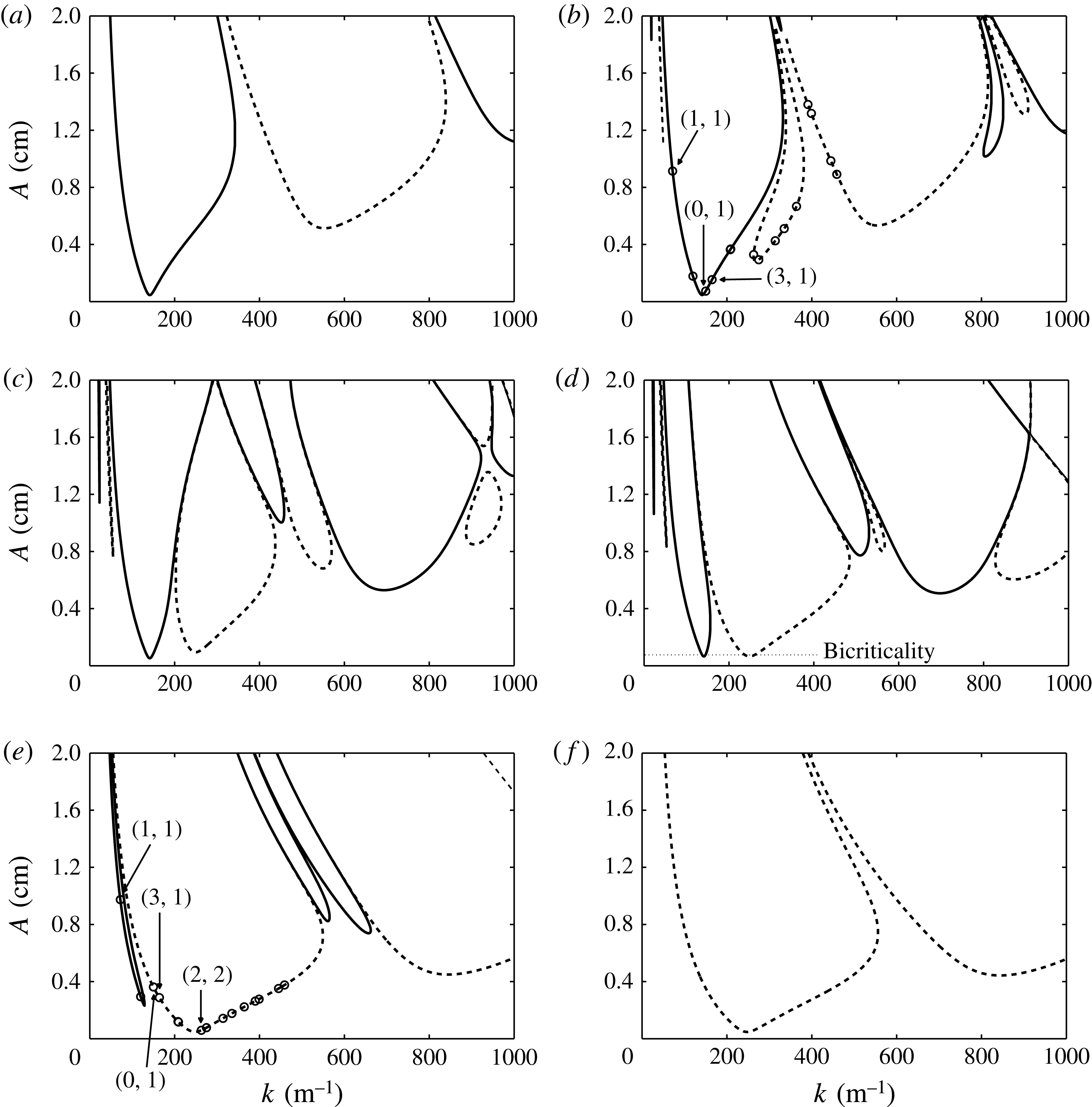
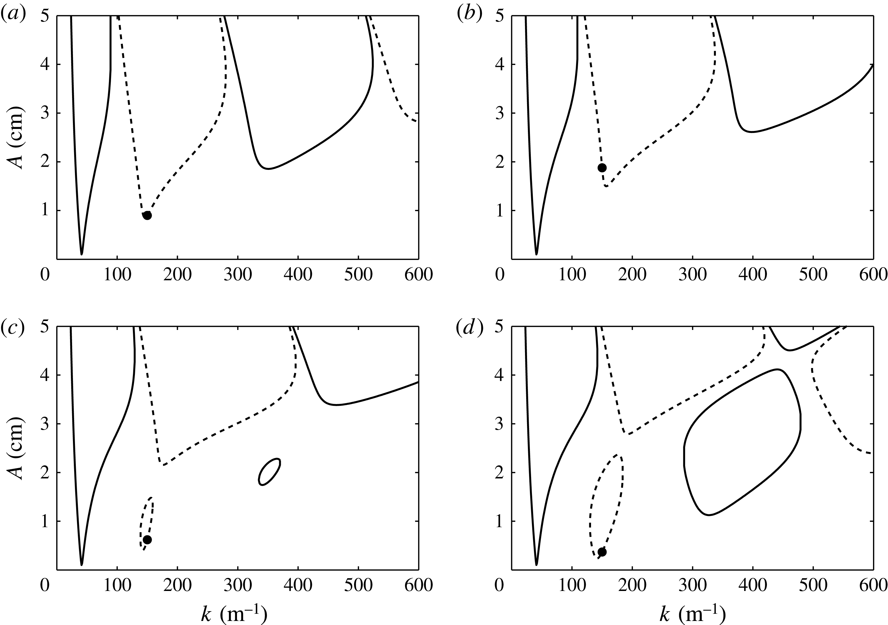
The eigenvalues of (3.3) are calculated using MATLAB’s eigenvalue routine, and repeated solution for a range of wavenumbers forms the familiar stability diagrams for a horizontally infinite bilayer. Figure 1(a–f) presents this calculation for several values of
 ${\it\chi}$
when
 $l/m=3/4$
, for the same fluid configuration as used in the experiments. Similar stability diagrams were first presented by Besson et al. (Reference Besson, Edwards and Tuckerman1996). In figure 1, panels (a) and ( f) represent the cases of single-frequency excitation for the pure
 $l{\it\omega}$
and
 $m{\it\omega}$
excitation of
 ${\it\chi}=0$
and 90°, and panels (b)–(e) display the results for four intermediate values to show the effect of two-frequency excitation. It can be observed that increase of the angle
 ${\it\chi}$
results in a dynamic process where the single-frequency tongues decrease in size while new tongues due to the second excitation frequency appear and then increase in size. The periodicity of these regions of instability alternates between harmonic (
 ${\it\alpha}=0$
) and subharmonic (
 ${\it\alpha}={\it\omega}/2$
), albeit in a manner more complex than the subharmonic–harmonic ordering in a single-frequency calculation. A nuance to the two-frequency calculation is that for
 ${\it\chi}=0$
or 90° for an even integer
 $l$
or
 $m$
there results a set of solely harmonic tongues. This is because a tongue that is subharmonic with respect to an even multiple of
 ${\it\omega}$
is viewed as harmonic with respect to
 ${\it\omega}$
. This is seen in figure 1( f), where excitation is at pure
 $4{\it\omega}$
, and the Floquet multiplier is
 ${\it\alpha}=0$
for each of the tongues. The lowest point on each diagram denotes both the threshold amplitude and wavenumber for the onset of instability in a laterally infinite system.
Linear stability of a horizontally infinite
 $(h_{1},h_{2})=(3.3,3.1~\text{cm})$
bilayer of FC-70 (
 ${\it\rho}_{1}=1888~\text{kg}~\text{m}^{-3}$
, 12 cSt) and silicone oil (
 ${\it\rho}_{2}=860~\text{kg}~\text{m}^{-3}$
, 1.5 cSt) at various angles
 ${\it\chi}$
: (a) 0°; (b) 10°; (c) 30°; (d) 46°; (e) 80°; ( f) 90°. These parameter values correspond to the experimental conditions and are used for the model calculation throughout the paper. Here,
 $l/m=3/4$
, the basic frequency
 $f={\it\omega}/2{\rm\pi}$
is 2.4 Hz, and the phase lag
 ${\it\phi}$
is 0°. Solid and dashed lines represent subharmonic and harmonic responses, respectively. The wavenumbers denoted by open circles in (b) and (e) are defined in (5.2) for the case of a cylinder of
 $R=2.55~\text{cm}$
. Acceleration due to gravity
 $g=9.81~\text{m}~\text{s}^{-2}$
.

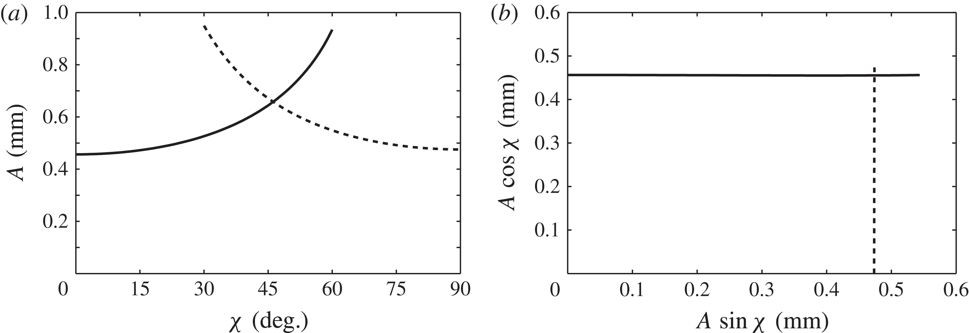
Figure 2(a) traces the minimum onset amplitude for the entire range of
 ${\it\chi}=0{-}90^{\circ }$
. The intersection of the subharmonic and harmonic thresholds at
 ${\it\chi}_{c}=46^{\circ }$
indicates a codimension-two point, and is of special interest. At these conditions, a wavenumber primarily excited by the
 $l{\it\omega}$
component is simultaneously neutrally stable with a wave excited primarily by the
 $m{\it\omega}$
component. The splitting of the two waves into different frequencies differs from the codimension-two points that arise in the single-frequency experiment where both spatial modes are locked to the same frequency (Kumar Reference Kumar1996; Ciliberto & Gollub Reference Ciliberto and Gollub1985). Experimentally, it was near this codimension-two point that Edwards & Fauve (Reference Edwards and Fauve1994) first uncovered the existence of quasi-patterns, and Kudrolli & Gollub (Reference Kudrolli and Gollub1996) later discovered so-called superlattice patterns.
Global minimum thresholds for the system of figure 1, presented as the (a) overall amplitude
 $A$
and (b) individual component amplitudes.

An important question inherent to two-frequency excitation is how the addition of a second frequency delays or advances the threshold obtained from a single-frequency calculation. In experiments, especially those of this paper, it is convenient to control the overall amplitude,
 $A$
, and thus figure 2(a) is useful. However, the adjustment of the primary-component threshold amplitude, either
 $A\text{cos}{\it\chi}$
or
 $A\sin {\it\chi}$
, due to the presence of the second component, is obscured by plotting the overall amplitude
 $A$
versus the angle
 ${\it\chi}$
. This interaction is revealed instead by plotting the component amplitudes
 $A\text{cos}{\it\chi}$
and
 $A\sin {\it\chi}$
against each other. The thresholds of figure 2(a) have been transformed in this manner in figure 2(b), and it can be observed that neither primary-component amplitude interacts significantly with the second component.
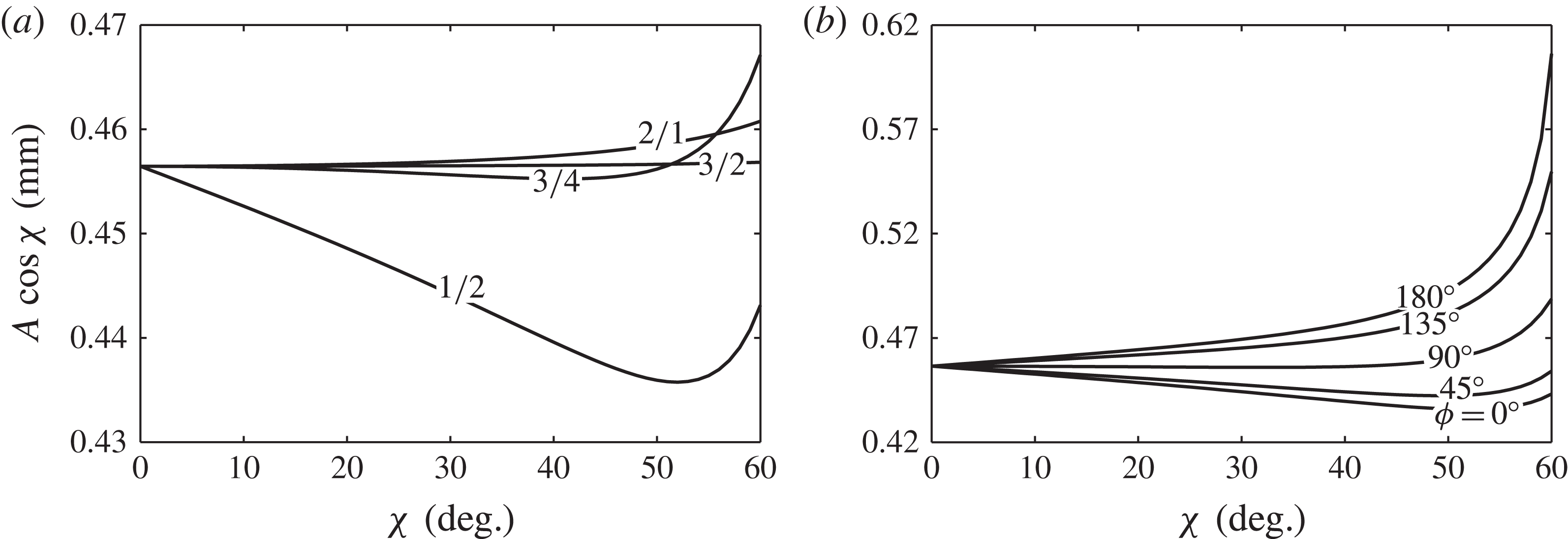
This is not always the case, as seen in figure 3(a), where the
 $l{\it\omega}$
component threshold has been plotted for several combinations of
 $l/m$
, with
 ${\it\phi}=0^{\circ }$
. Here the adjustment of the
 $l{\it\omega}$
primary-component threshold varies no more than a few per cent as the amplitude of the
 $m{\it\omega}$
component is increased. It seems difficult to predict a priori whether the addition of a second frequency will increase or decrease the primary-component threshold, yet figure 3 shows a general increase when
 $l<m$
and little change when
 $l>m$
. The degree to which a second frequency adjusts the critical threshold is a central question of this work, and we will later revisit this discussion in the context of the predictions for the single-mode regime.
Influence of two-frequency excitation on the
 $l{\it\omega}$
component amplitude for (a) various
 $l/m$
with
 ${\it\phi}=0$
and (b) various
 ${\it\phi}$
with
 $l/m=1/2$
.

While all two-frequency stability diagrams show some dependence on
 ${\it\phi}$
for the higher harmonic tongues, we have observed a significant effect of
 ${\it\phi}$
on the minimum threshold only for
 $1/2$
excitation, as shown in figure 3(b). Such an effect is absent for the
 $2/1$
,
 $3/4$
and
 $3/2$
cases of figure 3(a), whereas other integer-multiple excitations such as
 $1/3$
,
 $1/4$
or
 $1/5$
show a
 ${\it\phi}$
dependence. Previously, the experiments of Müller (Reference Müller1993) on pattern formation with
 $1/2$
excitation showed a significant effect of
 ${\it\phi}$
on the bicritical line separating harmonic and subharmonic patterns. Theoretically, Zhang & Viñals (Reference Zhang and Viñals1997b
) analysed subharmonic solutions of a linearly damped Mathieu equation subject to two-frequency excitation using the method of multiple scales. They showed that a single
 ${\it\phi}$
-dependent term arose in the solvability condition at second order only for the frequency ratio
 $1/2$
, affecting the linear stability condition. Although we do not produce it here, an analysis of harmonic solutions yields a similar
 ${\it\phi}$
-dependent term at first order. For this reason we cite the work of Zhang & Viñals (Reference Zhang and Viñals1997b
) as additional support of the uniqueness of the
 $1/2$
excitation for its sensitivity to
 ${\it\phi}$
.
5. Linear thresholds for a bounded cylinder
A discretized cell does not necessarily have access to the wavenumber corresponding to the tongue minimum as in the laterally infinite system. Therefore, the model must be adapted to a finite cylindrical container by enforcing a sidewall boundary condition to effect the discretization. One possibility is that the interface remains pinned to a fixed point on the sidewall, which can be experimentally realized by filling a container to its sharp brim. Unfortunately, the condition does not lead to separable horizontal eigenfunctions (see Benjamin & Scott Reference Benjamin and Scott1979). Recently, Kidambi (Reference Kidambi2013) has successfully incorporated this condition into a theory for inviscid Faraday waves and has detailed the means to solve the coupled linear system.
The stress-free condition, which leads to wavenumber discretization, was first applied by Benjamin & Ursell (Reference Benjamin and Ursell1954) to compare their single-mode experiment to an inviscid model. The condition implies that the interface moves freely while maintaining 90° contact with the sidewall, and, to date, all single-mode experiments have been designed to resemble this behaviour. Stress-free sidewalls were applied to the Kumar & Tuckerman (Reference Kumar and Tuckerman1994) model by Batson et al. (Reference Batson, Zoueshtiagh and Narayanan2013), and here the implications for the two-frequency excitation will be presented. For a cylinder with stress-free sidewalls, the perturbations must satisfy
 $$\begin{eqnarray}\left(\frac{\partial ^{2}}{\partial r^{2}}+\frac{1}{r}\frac{\partial }{\partial r}+\frac{1}{r^{2}}\frac{\partial }{\partial {\it\theta}}+k_{u,v}^{2}\right){\it\zeta}_{u,v}=0,\end{eqnarray}$$
which can then be decomposed as
 $$\begin{eqnarray}{\it\zeta}_{u,v}=J_{u}(k_{u,v}r)\sin u{\it\theta},\end{eqnarray}$$
where
 $k_{u,v}$
is the
 $v$
th zero of
 $J_{u}^{\prime }(k_{u,v}R)$
. The indices,
 $u$
and
 $v$
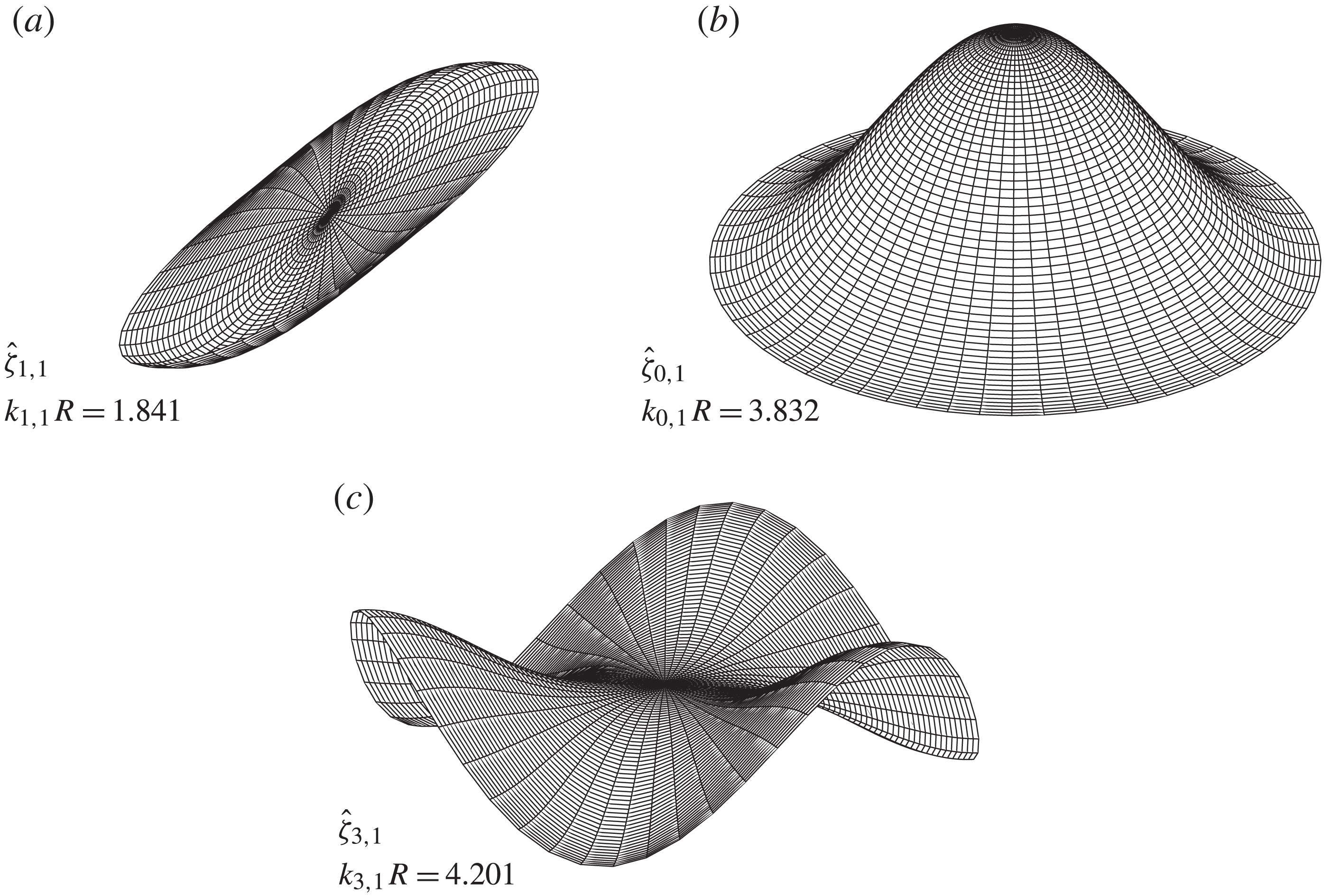
, indicate the number of azimuthal and radial nodes, respectively. Imposing this constraint discretizes the wavelengths available to the system and also specifies a waveform that depends on the shape of the container. Three examples of modes satisfying the stress-free condition, along with their dimensionless wavenumbers
 $k_{u,v}R$
, are depicted in figure 4.
Spatial forms of the
 $(1,1)$
,
 $(0,1)$
and
 $(3,1)$
cylindrical modes that satisfy the stress-free condition.

Discretized wavenumbers accessible to an
 $R=2.55~\text{cm}$
cylinder have been labelled on figure 1(b,e) to illustrate the difference in wavenumber selection between a finite container and an infinite system. The thresholds corresponding to the waves of figure 4 have been labelled, and it can be seen that at
 ${\it\chi}=10^{\circ }$
, the
 $(0,1)$
mode is excited first. In the discrete system, a mode is excited for a band of frequency or
 ${\it\chi}$
, as adjustment of either parameter causes the tongues of figure 1 to shift, until a neighbouring mode becomes the least stable. Codimension-two points are thus created at the boundaries of frequency or
 ${\it\chi}$
bands. The thresholds for several mode frequency bands for single-frequency excitation were studied by Batson et al. (Reference Batson, Zoueshtiagh and Narayanan2013), and in this work such bands will be studied for finite values of
 ${\it\chi}$
.
5.1. Discretized frequency bands
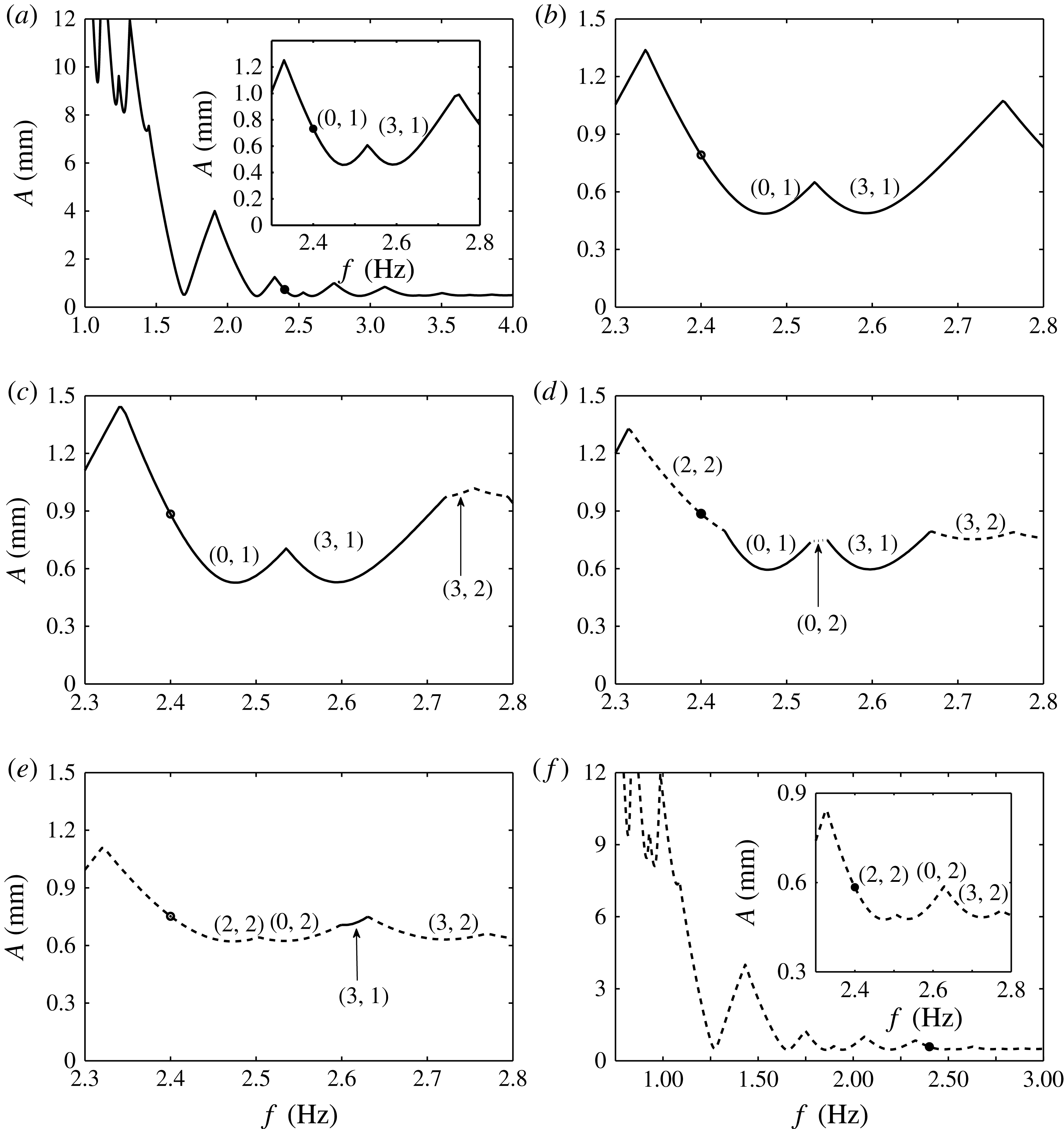
In order to detail the nature of the frequency bands in a discretized system excited by two frequencies, consider figure 5, where the frequency dependence of the thresholds is given for several values of
 ${\it\chi}$
when
 $l/m=3/4$
, as an example. Here, the single-frequency systems are depicted for
 ${\it\chi}=0^{\circ }$
in figure 5(a) and
 ${\it\chi}=90^{\circ }$
in figure 5( f), which are identical upon proper scaling of the basic frequency
 ${\it\omega}$
. A sequence of dips in the threshold in each panel is present, corresponding to different cell modes. The cusps in the threshold therefore represent codimension-two points, where two different cell modes are simultaneously unstable.
Stability of the
 $l/m=3/4$
system of figure 1 with stress-free cylindrical (
 $R=2.55~\text{cm}$
) discretization at various angles
 ${\it\chi}$
: (a) 0°; (b) 20°; (c) 30°; (d) 40°; (e) 50°; ( f) 90°. The filled circles track the threshold for fixed
 $f=2.4~\text{Hz}$
, and correspond to the marked thresholds in figure 6(a).

To investigate the effect of two-frequency excitation, we focus on the frequency range of 2.3–2.8 Hz, where the
 $(0,1)$
and
 $(3,1)$
modes are excited in the
 ${\it\chi}=0^{\circ }$
system, and the
 $(2,2)$
,
 $(0,2)$
and
 $(3,2)$
modes are excited in the
 ${\it\chi}=90^{\circ }$
system (see the insets of panels (a) and (f) in figure 5). Increase in
 ${\it\chi}$
from 20° to 50°, as shown in panels (b)–(e), depicts a dynamic process by which the
 ${\it\chi}=0^{\circ }$
frequency bands (solid line) give way to the
 ${\it\chi}=90^{\circ }$
bands (dashed line). At
 ${\it\chi}=20^{\circ }$
in figure 5(b), the same modes are excited as in the inset of panel (a), then frequency bands at which
 $(3,2)$
and
 $(1,3)$
modes due to the
 $4{\it\omega}$
excitation appear at
 ${\it\chi}=30^{\circ }$
in (c), followed by the addition of
 $(2,2)$
and
 $(0,2)$
modes at
 ${\it\chi}=40^{\circ }$
in (d). For
 ${\it\chi}=50^{\circ }$
in figure 5(e), only a small
 $(3,1)$
mode band due to the
 $3{\it\omega}$
excitation remains, and further increase results in a system where only modes excited primarily by the
 $4{\it\omega}$
component remain.
5.2. Discretized
 ${\it\chi}$
bands

The influence of a second frequency component on the primary
 $l{\it\omega}$
component threshold is studied by fixing the basic frequency
 ${\it\omega}$
and varying the mixing angle
 ${\it\chi}$
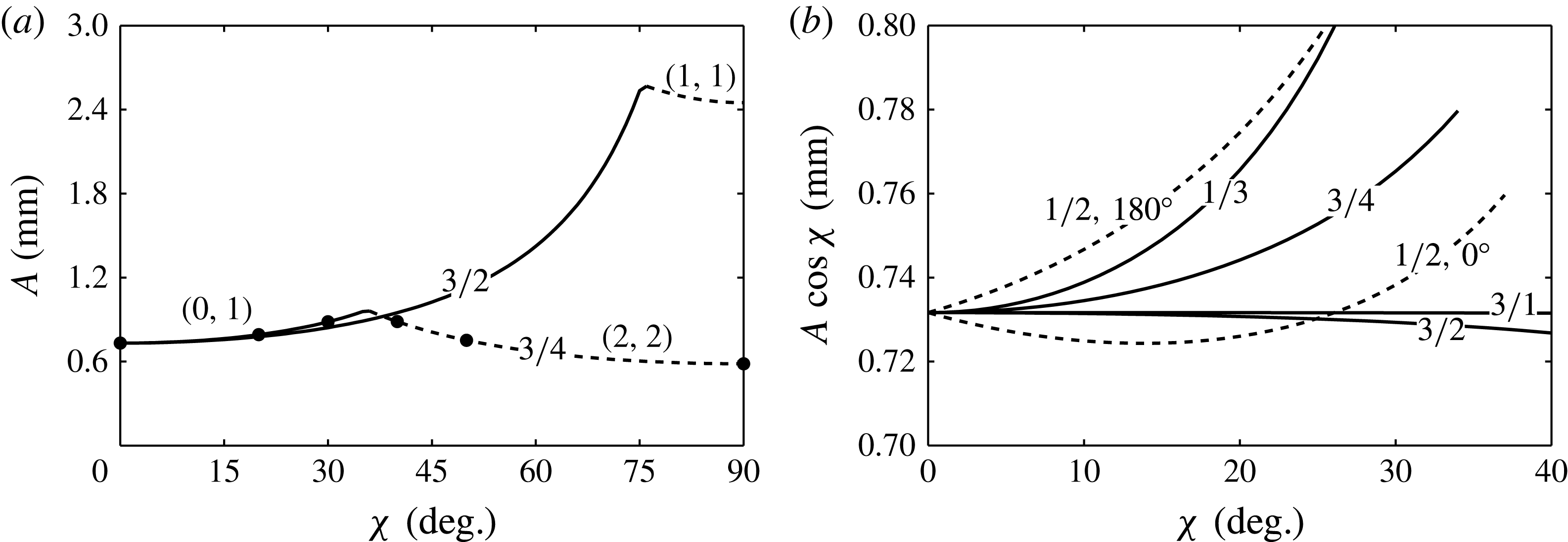
. Typical results are presented in figure 6(a) for both
 $l/m=3/4$
and
 $3/2$
excitation with
 $f=2.4~\text{Hz}$
. It is seen that the threshold for each case consists of two
 ${\it\chi}$
bands that excite different modes, joined by a codimension-two point at
 ${\it\chi}={\it\chi}_{c}$
. For values of
 ${\it\chi}<{\it\chi}_{c}$
, the
 $(0,1)$
mode is primarily excited by the
 $3{\it\omega}$
component for both excitations of figure 6(a). Above
 ${\it\chi}_{c}$
, the
 $(2,2)$
and
 $(1,1)$
modes are primarily excited by the
 $4{\it\omega}$
and
 $2{\it\omega}$
, respectively. Neither of the curves in figure 6(a) shows significant dependence upon the phase angle
 ${\it\phi}$
.
Fixed basic frequency (
 $f=2.4~\text{Hz}$
) stability for the cylindrical system of figure 5: (a) overall threshold amplitudes
 $A$
with
 $l/m=3/2$
and
 $3/4$
,
 ${\it\phi}=0^{\circ }$
; and (b) primary
 $l{\it\omega}$
component amplitudes with various
 $l/m$
(
 ${\it\phi}=0^{\circ }$
except for
 $l/m=1/2$
) for the system of figure 1 with cylindrical (
 $R=2.55~\text{cm}$
) stress-free discretization. The filled circles in (a) correspond to the thresholds as marked in figure 5(a–f).

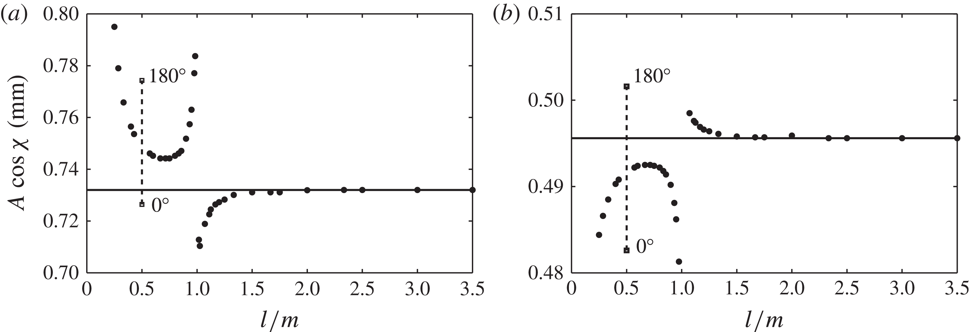
Primary
 $l{\it\omega}$
component thresholds for various frequency ratios
 $l/m$
at fixed
 ${\it\chi}=20^{\circ }$
and fixed primary-component frequencies of (a) 7.2 Hz and (b) 7.65 Hz. Only the
 $l/m=1/2$
thresholds depend upon
 ${\it\phi}$
, which vary monotonically between the labelled
 ${\it\phi}=0$
and 180° points.

As was first discussed for a laterally infinite system in figure 2, the behaviour of the overall amplitude
 $A$
at criticality does not reveal the effect of a second frequency on the primary-component threshold. To isolate this behaviour we replot the amplitudes
 $A\text{cos}{\it\chi}$
for the
 $(0,1)$
mode
 ${\it\chi}$
bands of figure 6(a) in figure 6(b). Here, the primary-component threshold increases with
 ${\it\chi}$
for
 $3/4$
excitation and decreases for
 $3/2$
excitation. Similar adjustment is seen for
 $1/3$
and
 $3/1$
excitation of the
 $(0,1)$
mode. In each of these excitations, addition of a higher/lower-frequency component increases/decreases the
 $l{\it\omega}$
component threshold. An exception to this classification is the
 $1/2$
excitation, which can either increase or decrease the
 $l{\it\omega}$
threshold, and shows dependence upon the phase lag
 ${\it\phi}$
.
To further differentiate between the addition of a higher (
 $l<m$
) or lower (
 $l>m$
) frequency, we present the
 $l{\it\omega}$
component threshold at which the
 $(0,1)$
mode is excited for several frequency ratios at fixed
 ${\it\chi}=20^{\circ }$
in figure 7. Many frequency ratios
 $l/m$
have been included here only to clarify trends in the threshold adjustment, and will not be considered elsewhere in the study. The frequencies are
 $l{\it\omega}/2{\rm\pi}=7.2~\text{Hz}$
in figure 7(a) and 7.5 Hz in figure 7(b), which correspond to conditions above (tuned) and below (detuned) the
 $(0,1)$
mode natural frequency. It is clearly seen that the sign of the adjustment to the
 $l{\it\omega}$
component threshold depends upon whether
 $l/m$
is greater than or less than 1, and also on whether the mode is tuned or detuned. This behaviour occurs because addition of a second frequency produces a slight shift in the natural frequency of a mode, to lower frequencies when
 $l<m$
and to higher frequencies when
 $l>m$
. The adjustment to the threshold amplitude at the new natural frequency is very slight. While this adjustment becomes more pronounced as the mode tuning or detuning is increased, it remains quite small relative to the single-frequency threshold, viz. figures 6(b) and 7(a,b). A key two-frequency experimental result that will be presented is that the nonlinear response of the system is significantly altered even when the linear threshold is not. Next we discuss a case where both the amplitude and phase of the second component have a significant effect on the primary-component threshold.
5.3. The case of
$l/m=1/2$
excitation showing strong
${\it\phi}$
dependence


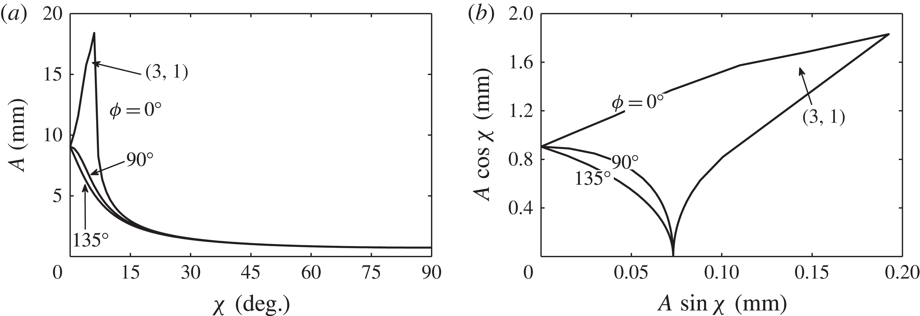
Strong dependence of the threshold upon the phase lag
 ${\it\phi}$
is seen for
 $1/2$
excitation of harmonic modes. That is,
 ${\it\omega}$
and
 $2{\it\omega}$
components are used to simultaneously excite the same mode harmonically and subharmonically, respectively. In figure 8(a,b) we present the overall and component threshold amplitudes for
 $1/2$
excitation for three values of
 ${\it\phi}$
. The basic frequency has been set to
 $f=3.6~\text{Hz}$
, such that the
 $(0,1)$
mode is harmonically excited by the
 ${\it\omega}$
component, and subharmonically excited by the
 $2{\it\omega}$
component. As a result, a codimension-two point between two different cell modes does not appear in this system. With
 ${\it\phi}=0^{\circ }$
, it can be seen that the
 $(0,1)$
mode threshold diverges for small
 ${\it\chi}$
, and there exists a
 ${\it\chi}$
band at significantly higher amplitudes where the system instead chooses a
 $(3,1)$
mode. The other sets of thresholds presented for
 ${\it\phi}=90$
and 135° do not exhibit this divergence in the threshold, although both still depend noticeably on
 ${\it\phi}$
.
Fixed-frequency (
 $f=3.6~\text{Hz}$
) stability of the cylindrical system for
 $l/m=1/2$
excitation: (a) overall threshold amplitudes
 $A$
with
 ${\it\phi}=0$
, 90 and 135°; and (b) corresponding
 $l{\it\omega}$
component thresholds. The
 $(0,1)$
mode is excited for each
 $l/m$
over the entire range of
 ${\it\chi}$
except for
 ${\it\chi}=[4,7^{\circ }]$
for
 ${\it\phi}=0^{\circ }$
where the
 $(3,1)$
mode is excited. The disparity in the axis scales of (b) emphasizes the significance of the small-
 ${\it\chi}$
behaviour.

The explanation for this divergence in the
 ${\it\phi}=0$
threshold in figure 6(b) is aided by figure 9(a–d), where the stability diagrams are presented for values of
 ${\it\chi}=0$
, 4, 8 and 12°. It is evident that addition of the
 $2{\it\omega}$
component produces a profound effect on the second, third and fourth tongues of figure 9(a). Circles are used to denote the wavenumber (
 $150.2~\text{m}^{-1}$
) and thresholds at which the
 $(0,1)$
mode is excited harmonically. Then, in figure 9(b), with
 ${\it\chi}=4^{\circ }$
, the harmonic tongue is damped considerably as slight amounts of the
 $2{\it\omega}$
component are added, accounting for the sharp jump observed in figure 6(b). The sharp decrease then occurs due to the creation of ‘islands’ of instability as seen for
 ${\it\chi}=8$
and 12° in figure 9(c,d). The damping of the second tongue and subsequent appearance of islands does not occur for the cases of
 ${\it\phi}=90$
or 135°. Islands can also be observed in figure 1 and in the stability diagrams of Besson et al. (Reference Besson, Edwards and Tuckerman1996). In each of these cases, the islands form by ‘pinching’ of the new tongues created by the
 $m{\it\omega}$
component, as seen in figure 1(c,d). However, the
 $1/2$
case presented here is different because the
 $2{\it\omega}$
component does not generate new tongues. Instead, the original single-frequency tongues of figure 9(a) are directly modified by the
 $2{\it\omega}$
component, which leads to island formation.
Stability of the horizontally infinite system with
 $f=3.6~\text{Hz}$
,
 $l/m=1/2$
,
 ${\it\phi}$
of 0° and varying
 ${\it\chi}$
: (a) 0°; (b) 4°; (c) 8°; (d) 12°.

The effect of
 ${\it\phi}$
in this example is significant and well within the level of detection of our experiment. We now set out to provide experimental evidence of this effect in addition to other aspects of the two-frequency theory, in a manner similar to that conducted by Batson et al. (Reference Batson, Zoueshtiagh and Narayanan2013) for the single-frequency theory. Specifically, experimental data sets will be presented and compared to the predictions of figures 5, 6 and 8. We will also present bifurcation data in which we have measured the nonlinear response of the system. To these ends, we re-introduce the experimental system that was developed in addition to the novel methods used for characterization of the vibrational input signal.
6. Experimental method
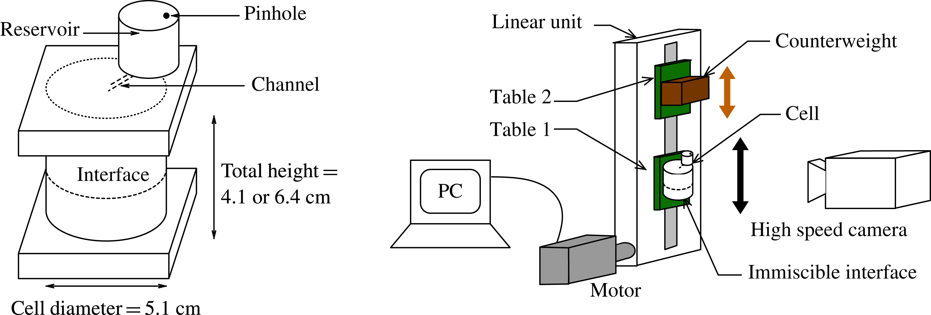
The experiments were conducted using an identical cylindrical cell and fluid combination as in Batson et al. (Reference Batson, Zoueshtiagh and Narayanan2013), cf. figure 10. The cell was constructed by capping a cylindrical glass tube of wall thickness
 ${<}3~\text{mm}$
with machined trenches in acrylic plates. Bolts were used with O-rings to form a seal, yielding a container of radius 2.55 cm and height of 6.4 cm. A small-diameter hole of less than 1 mm was bored through the upper plate connecting to an external reservoir. Overfilling the container into this reservoir produced a fully filled cell whereby bubbles and leaks due to fluctuations of the ambient conditions were prevented. Air was allowed to enter and leave the reservoir through a tiny pinhole. This construction also permitted the cell to remain filled, avoiding removal or addition of fluid over the duration of the run.
Test cell and the electromechanical shaker.

As in the earlier work, the test fluids were Fluorinert FC-70 and a 1.5 cSt silicone oil. These two fluids produce an interface whose contact line generates an apparently free motion over the glass sidewalls, closely approximating the stress-free sidewall condition required by the model. The fluid densities, measured with pycnometers, were
 $1888~\text{kg}~\text{m}^{-3}$
for FC-70 and
 $866~\text{kg}~\text{m}^{-3}$
for the silicone oil. We used the reported values of 12 cSt for FC-70 and 1.5 cSt for the silicone oil, with an interfacial tension of
 $7~\text{dyn}~\text{cm}^{-1}$
(Someya & Munakata Reference Someya and Munakata2005) in the calculations required by the model. Sensitivity analysis has been conducted to show that reasonable adjustment of these values by
 $\pm 10\,\%$
produces little change in the linear predictions.
6.1. Electromechanical shaker
Aside from the fluid choices and cell design, the critical aspect of the experimental design was control of the parametric excitation produced by the electromechanical shaker. The set-up is the same as that used by Batson et al. (Reference Batson, Zoueshtiagh and Narayanan2013), and its mechanical details are provided by Yoshikawa et al. (Reference Yoshikawa, Zoueshtiagh, Caps, Kurowski and Petitjeans2010). In summary, the set-up, pictured in figure 10, is designed to drive the test platform with sinusoidal speeds of up to
 $500~\text{cm}~\text{s}^{-1}$
and accelerations of
 $3500~\text{cm}~\text{s}^{-2}$
at frequencies between 0.1 and 10 Hz. The counterweight platform moves with phase opposite to the test platform in order to reduce transmission of vibrations to the set-up structure. The vibrational function
 $G(t)$
is directly programmed with the MotionPerfect 2 software interface, and the desired parameters
 $A$
,
 ${\it\chi}$
,
 $l/m$
and
 ${\it\phi}$
are independently chosen.
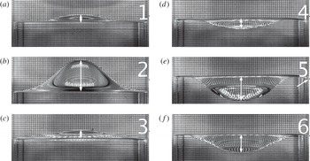
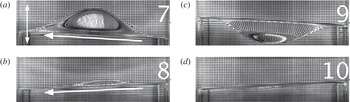
Sample images during one wave period of a
 $f=7.65~\text{Hz}$
subharmonic excitation of the
 $(0,1)$
mode. A grid is placed behind the cell to improve the wave contrast. All wave amplitudes reported in the work are taken to be half the length of the white arrows, which are used to denote the vertical distance from the central
 $(0,1)$
deflection to the sidewall interfacial contact line. The parametric signal is measured and analysed by recording a fixed point on the front of the cell, such as the small black marker pointed to in panel (e).

In the single-frequency experiments of Batson et al. (Reference Batson, Zoueshtiagh and Narayanan2013), we acknowledged that, while the measured frequency control was excellent (to within 0.1 % of the set point), the vibrational amplitude supplied to the experiment was normally less than the programmed input. Thus, to precisely determine the parametric input for each experiment, we directly measured the vibrational cell motion with high-speed imaging. While the amplitude of a single-frequency signal can be calculated simply by measuring the trough-to-crest displacement, Fourier analysis is necessary for a multiple-frequency signal. We will now detail these means by which we obtain the cell motion signal and precisely determine the parametric input. The excitation of a
 $(0,1)$
mode with a single frequency is used as an example, but the methods apply equally to two-frequency excitation. What we will show is that, in all cases, the parametric input to the system is determined to within 2 % of its actual value, which is then used to generate the model predictions to which the experiments are compared.
6.2. Wave deflection time series
Time series of both the cell motion and the interface deflection were obtained by recording the cell at 2000 frames per second (f.p.s.) using a stationary Photron SA3 camera. A level was used on both the camera and the experimental cell to ensure both that the cell motion was vertical and that the camera was directed normal to this motion. Sample images of single-frequency excitation of the
 $(0,1)_{sh}$
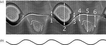
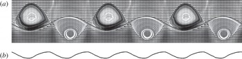
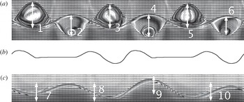
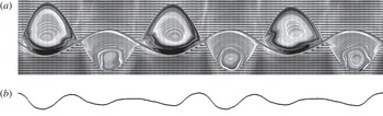
mode are presented in figure 11. A composite image of both the central wave deflection and the cell motion time series is presented in figure 12. Here, both the wave deflection and the cell motion time series are obtained by side-by-side stacking of a vertical slice of a single pixel width from each recorded image. To illustrate this, observe the correspondence between the white arrows in figure 11 and those in figure 12, and it becomes evident that the crests and troughs of figure 12 depict the time evolution of the central wave deflection of the
 $(0,1)$
mode. This time series is constructed from 1024 camera images, and, considering the frame rate and the excitation frequency of 7.65 Hz, the wavy lines of figure 12 correctly exhibit nearly four oscillations. In the results section, these series are transformed from the stationary laboratory frame to the vertically oscillating frame. Notably, this transformation renders the wavy lines from the back grid straight and more intuitively represents the wave amplitude in time (see figures 17, 20, 23 and 26).
(a) Time series data for the excitation depicted in figure 11. All images of time series data are created by horizontally stacking a single pixel-wide slice of data from images recorded at 2000 f.p.s. The numbered white arrows of this image directly correspond to data marked by the white arrows in the images of figure 11. The bottom half of this image is time series data obtained from the vertical motion of the black marker on the far right of the images of figure 11 for the duration of the excitation. (b) The harmonic content of the parametric input to each experiment is calculated via fast Fourier transform of this signal.

Quantitatively, we use these data to measure the maximum deflection of a saturated wave, which allows us to characterize bifurcation of the system with respect to the critical parameters
 $A$
,
 ${\it\chi}$
and
 ${\it\phi}$
. Qualitatively, while the time series data generally do not contain information about the spatial structure of the wave, observe that the reflection patterns in both the crests and the troughs of figure 12 are nearly identical. This is remarkable given the complexity of light refraction across the interface, and suggests that the wave is very nearly periodic from crest to crest and from trough to trough. On the other hand, in the results section, we will conclude that two-frequency waves are not periodic in this manner because we observe that the amplitudes and reflection patterns are not identical from crest to crest or from trough to trough.
6.3. Cell motion time series and digitization
The cell motion at the bottom of figure 12 was obtained by recording the motion and stacking the time series of a fixed point on the exterior of the cell. To facilitate quick and automated processing, the fixed point was created by attaching a strip of white paper with a very thin (
 ${\leqslant}1~\text{mm}$
) horizontal line to the cell. This is denoted by a black tick and is pointed out by the arrow in the fifth image of figure 11. The sharp contrast of the image allowed quick and repeatable conversion from greyscale to the depicted binary image. We used ImageJ’s ‘Skeletonize’ command to trim the signal to a single black pixel per time frame, representing the cell position at each step. Finally, the image is processed in MATLAB to obtain a vector of the cell displacement sampled at the frame rate of 2000 f.p.s. We estimate that the error associated with this digitization is no more than a pixel, which equates to less than 2 % for the smallest amplitude measurements (image resolution varied between 200 and
 $300~\text{pixels}~\text{cm}^{-1}$
). Otherwise the error associated with the method decreases linearly with the signal amplitude and is less than 1 % for the vast majority of the presented data. To calculate harmonic content and the parameters
 $A$
,
 ${\it\chi}$
and
 ${\it\phi}$
, we use MATLAB’s discrete Fourier transform routine for a single period of the cell displacement (for example, 784 frames of a 2.55 Hz excitation). By calculating the parametric input of a single period, we assume that the cell motion is constant for the duration of the experiment. This assumption was verified by analysing the motion at different times during an excitation and observing no change, for example, well before onset and after the saturation of a wave. In the next section we discuss the harmonic characterization for two example signals.
An alternative to consider for this type of problem is to use a MEMS-based accelerometer to measure the instantaneous acceleration felt by the cell, and incorporate this measurement into a feedback loop. Of course, this method also requires its own calibration. Instead, we have incorporated a posteriori analysis to characterize the oscillatory behaviour. Nevertheless, automated codes in both ImageJ and MATLAB place the limiting rate of analysis on the camera data transfer rate, which meant that about two minutes of time was necessary to fully determine the parametric input for a given experiment. Given that the growth and saturation of the instability has a delay time of its own, the cell motion analysis was seamlessly integrated into the experimental procedure and data sets such as the onset behaviour or bifurcation data were collected efficiently and analysed.
6.4. Cell motion Fourier analysis
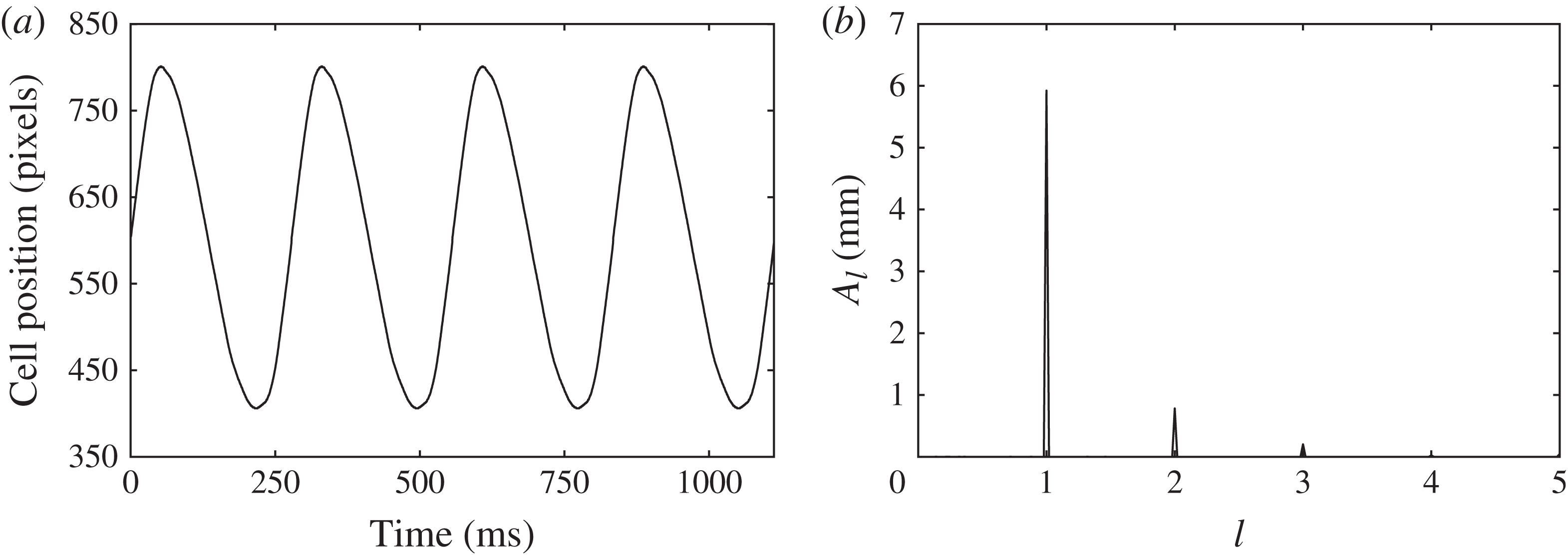
To detail the method by which the parametric input is characterized, we present the measured pixel displacement of the cell for four periods of a sample
 $1/2$
excitation (
 ${\it\omega}=3.6~\text{Hz}$
) and its Fourier spectrum in figure 13. The abscissa of the spectrum has been rescaled to present the frequencies as multiples of the basic frequency,
 ${\it\omega}$
. The peak amplitudes have been converted to real amplitudes, and are calculated as the square root of the product of the Fourier coefficient with its conjugate. Peaks appear precisely at the programmed frequencies of
 $l{\it\omega}$
and
 $m{\it\omega}$
, and this is consistent with all reported data. The angle
 ${\it\chi}$
evaluates to 7.53° and is calculated using the relation
 ${\it\chi}=\arctan (A_{m}/A_{l})$
, where
 $A_{l}$
and
 $A_{m}$
are the component amplitudes. Then the overall amplitude is 5.98 mm via
 $A=A_{l}/\!\text{cos}{\it\chi}=A_{m}/\!\sin {\it\chi}$
. The relative phase angle
 ${\it\phi}$
is 74.6° and is calculated using the angles of the complex Fourier coefficients.
Measured (a) parametric signal and (b) Fourier component amplitudes of a sample
 $l/m=1/2$
signal. The peak at
 $l=3$
in (b) indicates the presence of undesired harmonic content in the signal (a).

The final question about the electromechanical shaker output that must be addressed is the significance of undesired signal harmonics. We found that such harmonics consistently arose for low values of
 $A$
and high values of
 ${\it\chi}$
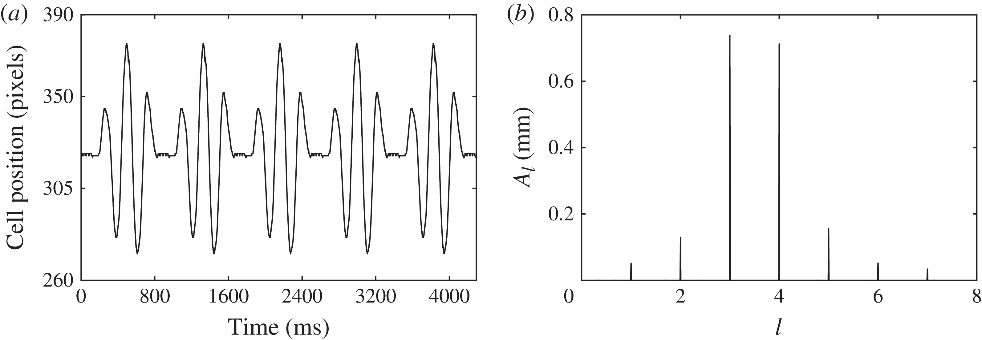
. To illustrate an extreme case, we present another signal and its Fourier spectrum in figure 14. Here, the parameters
 $[A,{\it\chi},{\it\phi}]$
for this
 $3/4$
signal (
 ${\it\omega}=2.33~\text{Hz}$
) are calculated to be
 $[1.03~\text{mm},44.0^{\circ },-6.3^{\circ }]$
. The amplitudes of the undesired peaks appearing at frequencies of
 ${\it\omega}$
,
 $2{\it\omega}$
,
 $5{\it\omega}$
and
 $6{\it\omega}$
are far too small to excite modes of their own. However, in principle, these undesired components interact with the
 $l{\it\omega}$
and
 $m{\it\omega}$
components to alter the onset and the nonlinear dynamics of the instability. The only set of experiments we observed that exhibit an influence from an undesired component was the single-frequency harmonic excitation of the
 $(0,1)$
mode. Here we correlate fluctuations in the saturated wave response to the amplitude of the (undesired)
 $2{\it\omega}$
component in the input signal. We have already shown in figures 6 and 9 that this interaction can be significant, and this result further motivated us to study the
 $1/2$
excitation. Otherwise, within the accuracy of our measurement techniques, we do not observe significant effects due to these undesired components.
Measured (a) parametric signal and (b) Fourier component amplitudes of a sample
 $l/m=3/4$
signal. The peaks at
 $l=1$
, 2, 5, 6 and 7 in (b) all indicate undesired harmonic content in the signal (a).

6.5. Measurement of the onset of instability
The experimental onset of instability is difficult to characterize owing to the non-ideality of the sidewall meniscus and the nature of the bifurcation, both of which were discussed in detail by Batson et al. (Reference Batson, Zoueshtiagh and Narayanan2013). To summarize, the contact line behaviour of the immiscible fluids creates a complex three-phase problem with the glass sidewall. When the system is at rest, this behaviour presents itself as the formation of a tiny convex-down meniscus, indicating that silicone oil preferentially wets the sidewall compared to the FC-70. This acts as a source of imperfect bifurcation, as initializing oscillation of the system causes the emission of travelling waves to the interior of the interface when excitation is either above or below the instability threshold. The amplitudes of these waves are normally quite small, and the difference between a Faraday-stable and -unstable system is obvious and can be observed by eye. However, as discussed in Batson et al. (Reference Batson, Zoueshtiagh and Narayanan2013), these waves are amplified when the
 $(0,1)$
mode is excited harmonically, and can lead to ‘early’ observation of the linear onset. Additionally, the response of the wave amplitude near the threshold is quite small when the excitation frequency is higher than the natural frequency, consistent with supercritical bifurcation.
Therefore, to provide a better representation of the experimental onset, we will present two types of data. The first type corresponds simply to sets of stable and unstable conditions, as determined by eye. The experimental onset that may be compared to the model predictions is then inferred as the interpolation between these conditions. Nearest the onset, it was common for three to five minutes to pass before the instability would appear and grow. Thus a point was labelled as ‘unstable’ if this appearance was observed, and ‘stable’ if only the meniscus waves persisted after a sufficient wait. A significant effort was made to narrowly pinpoint the onset by reducing the gap between stable and unstable points as much as possible. This method improves considerably upon the work of Batson et al. (Reference Batson, Zoueshtiagh and Narayanan2013), where only unstable points were presented.
The second type of data we report is bifurcation of the saturated wave deflection
 $A_{W}$
for the
 $(0,1)$
mode with respect to the parametric amplitude
 $A$
or angle
 ${\it\chi}$
. These data allow us to demonstrate the subcritical and supercritical nature of the bifurcation. We take
 $A_{W}$
to be half the maximum vertical difference between the sidewall contact and the crest elevation, as indicated by arrow no. 2 in figures 11 and 12. By comparing this maximum amplitude from crest to crest in a time series, we are also able to draw conclusions about the periodicity of the saturated waves. The presence of the sidewall meniscus causes this method to give a finite, but small, reading for
 $A_{W}$
when there is no instability.
7. A brief report of single-frequency experiments
Before presenting results for two-frequency excitation, we review the experimental behaviour for single-frequency excitation using the data collection methods of this study. The onset behaviour of subharmonically excited
 $(2,1)$
and
 $(0,1)$
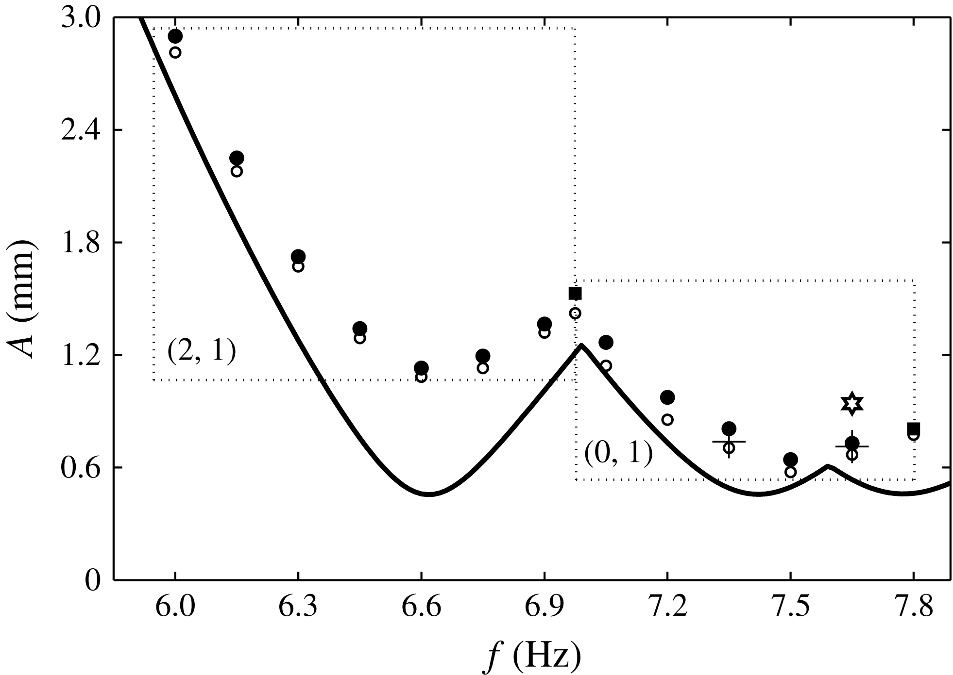
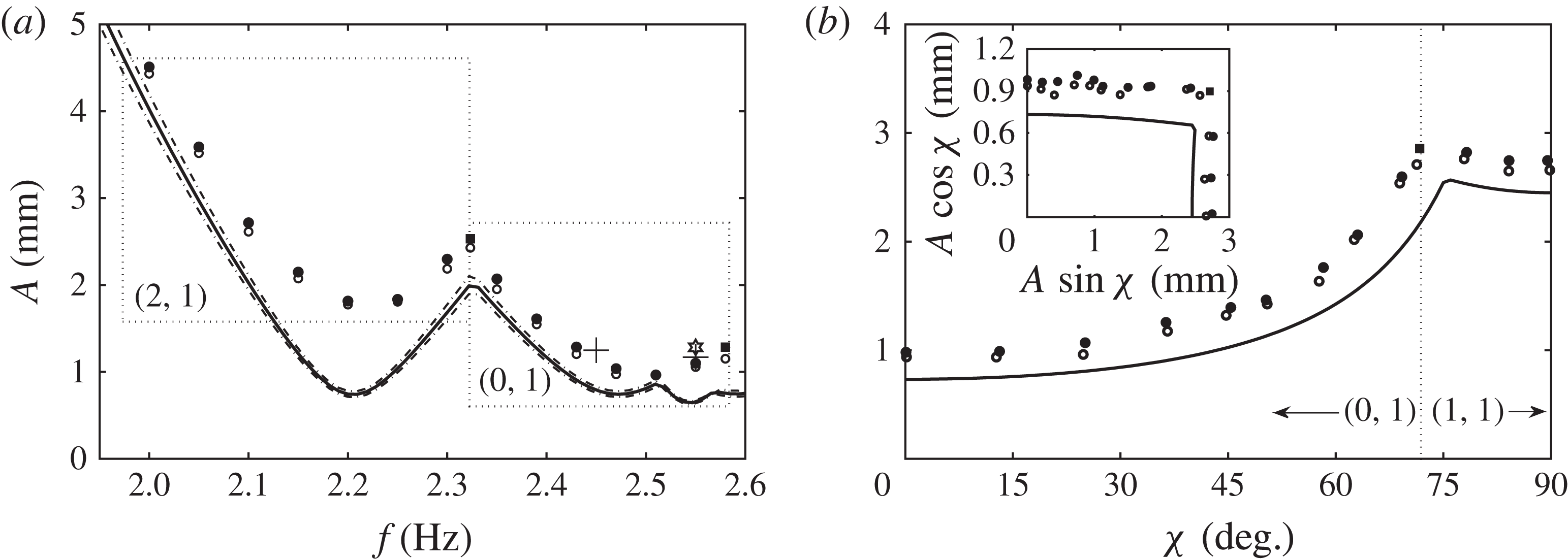
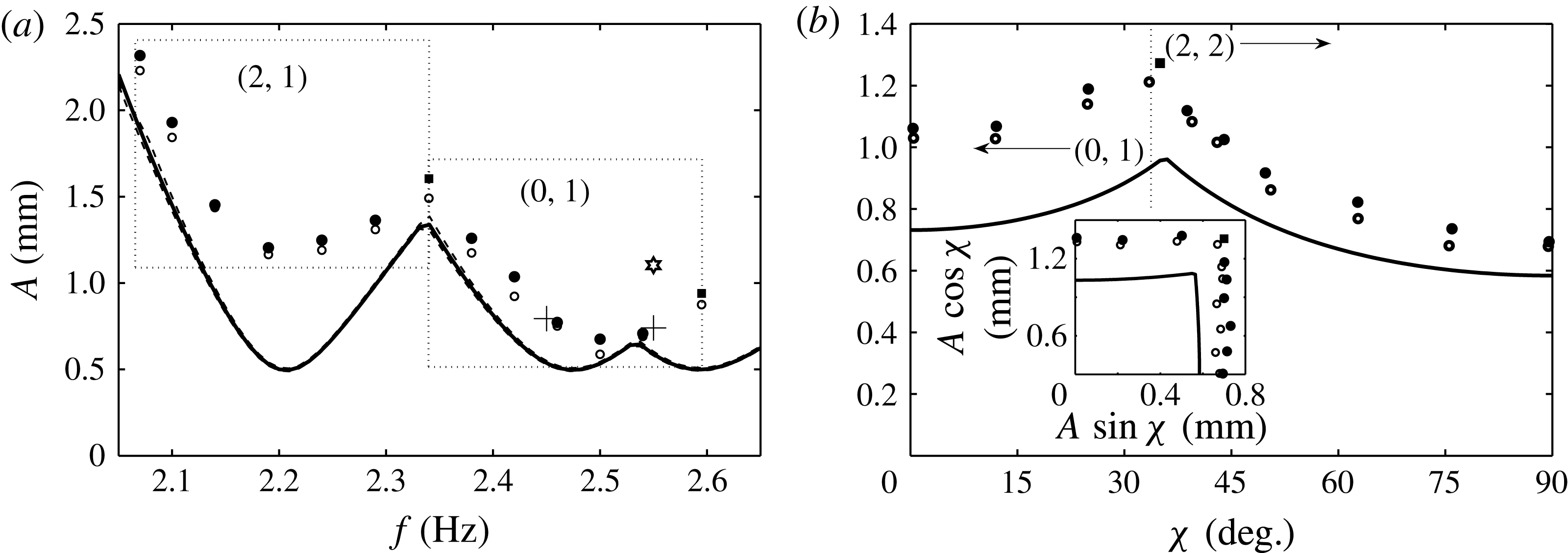
modes is presented in figure 15, where open/filled circles indicate stable/unstable conditions, and the solid line is the model prediction. Filled squares indicate conditions where simultaneous excitation of the two neighbouring modes was observed, and implies proximity to the codimension-two point. At 6.99 Hz, both
 $(2,1)$
and
 $(0,1)$
modes were observed, and both a
 $(0,1)$
and a
 $(3,1)$
mode were observed at the 7.8 Hz point. Interpolation between filled and unfilled points represents the threshold curve for the experimental system. Several experiments were performed at each frequency, and the data presented in figure 15 represent the stable and unstable conditions that most narrowly pinpoint the onset.
Comparison between the experiment and the linear stability model (solid line) for single-frequency excitation in the
 $R=2.55~\text{cm}$
cell. Open circles indicate conditions at which the instability was not observed. Filled circles indicate conditions in which a single mode was excited, filled squares indicate conditions where two modes were excited simultaneously. Dotted-line boxes are used to denote the excited mode for the grouped experimental data. The experimental parameters are the same as listed for the model in figure 1. The two crosses represent the threshold as indicated by the bifurcation data of figure 16, and the star marks the conditions at which the time series of figure 17 was obtained.

In order to properly interpret the agreement between the model and the two-frequency thresholds of this work, the findings of Batson et al. (Reference Batson, Zoueshtiagh and Narayanan2013) will first be reviewed and used to explain the results of figure 15. In this work it was demonstrated that the dissipation of the FC-70/1.5 cSt silicone oil system was dominated by bulk viscous effects, in stark contrast to the experiments of previous workers, who reported single-mode Faraday thresholds. As a result, the model quite remarkably predicted the system behaviour. However, residual sources of dissipation, unaccounted for by the model, make it unreasonable to expect an agreement as close to that seen by Bechhoefer et al. (Reference Bechhoefer, Ego, Manneville and Johnson1995), who verified the Kumar & Tuckerman (Reference Kumar and Tuckerman1994) theory for laterally large systems where such sidewall dissipative effects are of no consequence. Likewise, the results of this work ought not to be compared to those of Besson et al. (Reference Besson, Edwards and Tuckerman1996), who observed close agreement for the two-frequency case in a laterally large container. Bechhoefer et al. (Reference Bechhoefer, Ego, Manneville and Johnson1995) observed their agreement in shallow, round (
 $D=10~\text{cm},~h=1.0~\text{cm}$
) and square (
 $W=11.4~\text{cm},~h=0.24~\text{cm}$
) containers for wavenumbers greater than
 $2~\text{cm}^{-1}$
. They further reported loss of agreement at lower frequencies and higher wavelengths due to mode discretization. Lower frequencies were not investigated by Besson et al. (Reference Besson, Edwards and Tuckerman1996), who used a significantly larger circular container (
 $D=32~\text{cm},~h=0.3~\text{cm}$
) to excite wavelengths of
 $10~\text{cm}^{-1}$
using different two-frequency excitations.
Following Batson et al. (Reference Batson, Zoueshtiagh and Narayanan2013), the agreement between the model and the predictions in figure 15 is assessed by first considering that the model predicts a sequence of three modes: the
 $(2,1)$
mode at a natural frequency of 6.6 Hz, the
 $(0,1)$
mode at 7.4 Hz, and the
 $(3,1)$
mode at 7.8 Hz. It can then be seen that the experimental frequency bands for the
 $(2,1)$
and
 $(0,1)$
modes appear very close to the predictions; however, the
 $(0,1)$
band extends to higher frequencies, into the predicted
 $(3,1)$
mode band. It is also quickly observed that the experimental thresholds for both the
 $(2,1)$
and the
 $(0,1)$
modes lie above the model predictions. Closer inspection shows, arguably, greater deviation for the
 $(2,1)$
mode, which can be attributed to its sidewall wave nodes. The
 $(0,1)$
mode does not have such nodes. It is this deviation, which arises from the sidewall effects, that must be considered when analysing the two-frequency results.
Fourier analysis of the parametric signals in figure 15 revealed that the amplitude of the desired
 ${\it\omega}$
component constituted, on average, 88.4 % of the total Fourier content of the signal, and that a
 $3{\it\omega}$
component dominated the undesired content. The modification of the
 ${\it\omega}$
component threshold amplitude due to a
 $3{\it\omega}$
component was presented in figure 6(b) for 7.2 Hz excitation of the
 $(0,1)$
mode. If we assume that the average input to the experiment was a
 $l/m=1/3$
signal with a mixing angle
 ${\it\chi}=\arctan (12.6/88.4)=8.50^{\circ }$
, then the prediction of figure 6(b) is that the 7.2 Hz component threshold would rise by less than 1 %. Henceforth, we assume such undesired components make similarly insignificant modifications to the experimental onset, and we calculate the theoretical predictions based solely on the amplitudes of desired parametric components.
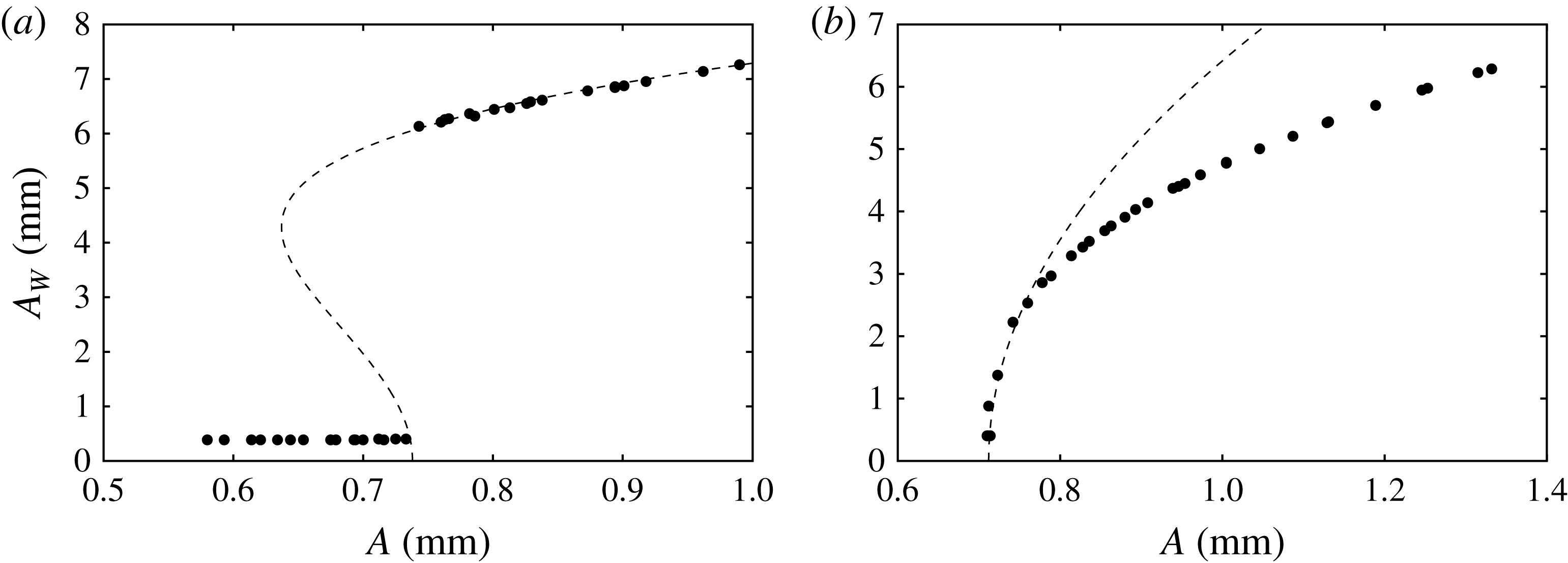
Saturated wave responses
 $A_{W}$
of the central
 $(0,1)$
mode deflection for the system presented in figure 15, excited at (a) 7.35 Hz and (b) 7.65 Hz. The parameters for the fit (7.1) are
 $[{\it\alpha},{\it\beta},A_{c}]=[-1.1\times 10^{-2},3.0\times 10^{-4},0.738]$
in (a) and
 $[7\times 10^{-3},0,0.712]$
in (b). Both fitting parameters
 $A_{c}$
are labelled on figure 15.

(a) Time series data for a
 $(0,~1)$
mode excited with
 $[\,f,~A]= [7.65~\text{Hz}$
,
 $0.94~\text{mm}]$
and (b) the input parametric signal. The image has been processed to present the series in the cell motion reference frame. The parametric input for this series is marked by the star in figure 15.

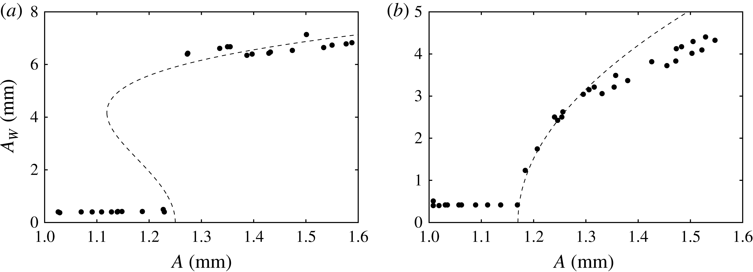
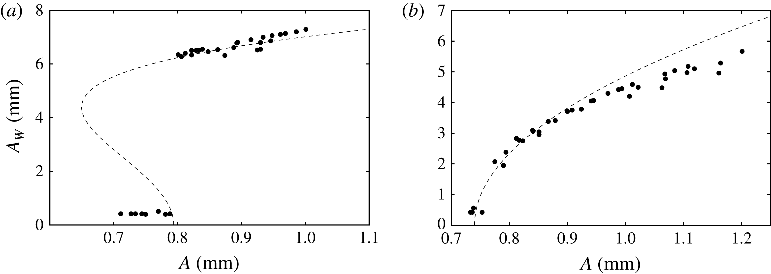
To characterize bifurcation of the instability, figure 16(a,b) presents the saturated wave responses for
 $(0,1)$
excitation at 7.35 and 7.65 Hz, that is, excitation below and above the natural frequency. Most remarkable is the difference in the response just after the instability, where, for the 7.35 Hz data, the system exhibits meniscus response up until the onset of
 $A=0.74~\text{mm}$
, and then at higher excitation the system responds with a discontinuous jump to a finite wave amplitude. In contrast, the 7.65 Hz response is continuous above the onset of
 $A=0.72~\text{mm}$
. This represents a transition from subcritical to supercritical bifurcation, which was elucidated theoretically by Douady (Reference Douady1990) via symmetry arguments for a generalized nonlinear oscillator. This transition, dependent on the sign of the frequency detuning, has been reported experimentally in several single-mode Faraday works (Henderson & Miles Reference Henderson and Miles1990; Tipton & Mullin Reference Tipton and Mullin2004; Das & Hopfinger Reference Das and Hopfinger2008). Similar behaviour will be reported in the two-frequency results. A fit of the data to a generalized form of the steady-state Landau equation (Grindrod Reference Grindrod1991; Strogatz Reference Strogatz2001),
 $$\begin{eqnarray}A-A_{c}={\it\alpha}A_{W}^{2}+{\it\beta}A_{W}^{4},\end{eqnarray}$$
is attempted by setting
 $A_{c}$
to the observed threshold and adjusting the parameters
 ${\it\alpha}$
and
 ${\it\beta}$
. The observed thresholds are marked by crosses in figure 15.
A time series for the saturated supercritical
 $(0,1)$
deflection and its measured cell displacement are pictured in figure 17. Here the
 $(0,1)$
mode has been excited at 7.65 Hz with an amplitude of
 $A=0.94$
mm (see the star in figure 15). The amplitude of the excitation is sufficiently close to the onset such that the wave remains periodic from crest to crest. This qualification is made strictly upon the observation that the maximum wave amplitude and the reflection patterns are constant from crest to crest in figure 17. Increase in the excitation amplitude naturally results in irregular dynamics, such as interface rupture.
Comparison between the experiment and the model for
 $l/m=3/2$
excitation for (a) average
 ${\it\chi}=51.9^{\circ }$
and (b) fixed
 $f=2.45~\text{Hz}$
. The dashed thresholds in (a) have been calculated for the minimum (49.8°) and maximum (51.9°) values of
 ${\it\chi}$
in this data set. The experimental data points are defined as was done for figure 15.

8. Two-frequency experimental results
The two-frequency results are organized as follows. We investigate two-frequency subharmonic excitation of the
 $(0,1)$
mode for both
 $l/m=3/2$
and
 $3/4$
, in a manner similar to that of the single-frequency case. The onset is initially characterized by varying
 ${\it\omega}$
with fixed
 ${\it\chi}$
, which yields data sets similar to the single-frequency data of figure 15. The effect of the
 $m{\it\omega}$
component on the onset is then further characterized with data obtained for fixed
 ${\it\omega}$
and variable
 ${\it\chi}$
. For both frequency ratios, the
 $(0,1)$
mode is primarily excited by the
 $3{\it\omega}$
component for
 ${\it\chi}<{\it\chi}_{c}$
. Thus both cases of the second frequency being higher (
 $m>l$
) and lower (
 $m<l$
) than the primary component are considered. In neither case do the two frequencies interact significantly with the onset of instability (see figures 6
b and 7), yet the nonlinear response is altered. The phase lag
 ${\it\phi}$
is not observed to have any effect on either the experimental or the model predictions for these conditions. The two-frequency results are therefore concluded with an investigation where the effect of
 ${\it\phi}$
is significant, which we demonstrate for harmonic excitation of the
 $(0,1)$
mode with
 $l/m=1/2$
.
8.1. The
$3/2$
subharmonic excitation of the
$(0,1)$
mode


Figures 18–20 present experimental data for
 $3/2$
parametric excitation. A data set similar to figure 15 is presented in figure 18, where the variable-frequency onset behaviour is probed for an average angle of
 ${\it\chi}=51.9^{\circ }$
. The dashed lines have been included along with the model prediction for the average (solid line) to reflect the minimum and maximum values of
 ${\it\chi}$
in this data set. The associated variance in the model prediction is small, and it can be concluded that the agreement with the data appears to be identical to that for the single-frequency data of figure 15. Here the
 $(2,1)_{sh}$
and
 $(0,1)_{sh}$
modes are primarily excited by the
 $3{\it\omega}$
component, in general agreement with the model predictions. However, the model does in fact predict the appearance of a
 $(1,1)_{sh}$
mode in resonance with the
 $2{\it\omega}$
component at
 $f=2.55~\text{Hz}$
, whereas it is the
 $(0,1)_{sh}$
mode that is first excited. This discrepancy results from larger sidewall dissipation of the
 $(1,1)$
mode relative to the
 $(0,1)$
mode. Two multi-mode excitations near the codimension-two points are observed, the first consisting of the
 $(2,1)$
and the
 $(0,1)$
mode at 2.33 Hz, and the second consisting of the
 $(0,1)$
mode and the
 $(3,1)$
mode at 2.58 Hz.
Saturated wave response of the central
 $(0,1)$
mode deflection for
 $l/m=3/2$
excitation at (a) 2.45 Hz and (b) 2.55 Hz, as marked in figure 18. Parameters for the fit (7.1) are
 $[{\it\alpha},{\it\beta},A_{c}]=[-1.5\times 10^{-2},4.3\times 10^{-4},1.25]$
in (a) and
 $[1.3\times 10^{-2},0,1.17]$
in (b). Both fitting parameters
 $A_{c}$
are labelled on figure 18.

(a) Time series data for a
 $(0,1)$
mode excited with
 $[l/m,f,A,{\it\chi}]=[3/2,2.55~\text{Hz},1.28~\text{mm},50.7^{\circ }]$
and (b) the input parametric signal. Two periods of the
 $f=2.55~\text{Hz}$
excitation are depicted. These parametric conditions are marked by the star in figure 18.

The data of figure 18(a) exhibit good agreement between the model and the experiment for a fixed value of
 ${\it\chi}$
. Figure 18(b) describes the threshold behaviour of the system for
 $3/2$
excitation for all values of
 ${\it\chi}$
, where the onset of instability is reported for a fixed frequency of 2.4 Hz. Looking first at
 ${\it\chi}=0^{\circ }$
, corresponding to the single-frequency 7.2 Hz data of figure 15, it is seen that the discrepancy between the model and the data remains constant for the entire range of
 ${\it\chi}$
for which the
 $(0,1)$
mode is excited. The discrepancy again results from sidewall dissipation that is unaccounted for, and thus we conclude that the model is equally satisfactory at predicting the two-frequency onset of instability as previously observed for the single-frequency case. In figure 18(b), the
 $(0,1)$
mode is excited in the experiment until a value of about
 ${\it\chi}_{c}=70^{\circ }$
, where both the
 $(0,1)$
and a
 $(1,1)$
mode are excited. The
 $(1,1)$
mode is then excited primarily by the
 $2{\it\omega}$
component for
 ${\it\chi}>{\it\chi}_{c}$
. These thresholds have been replotted in the inset of figure 18(b) as the individual component amplitudes
 $A\text{cos}{\it\chi}$
and
 $A\sin {\it\chi}$
. It is difficult to say whether or not the experimental thresholds show this interaction (which is predicted to be very small). The phase lag
 ${\it\phi}$
is calculated to have virtually no effect on the thresholds of figure 18(a) or (b), and no experimental evidence was found to claim otherwise.
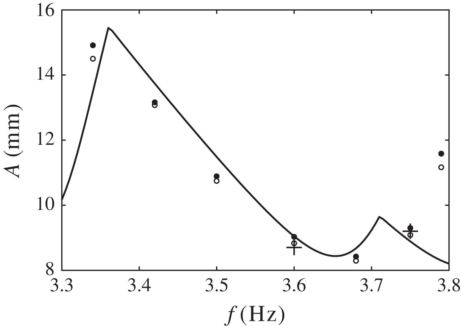
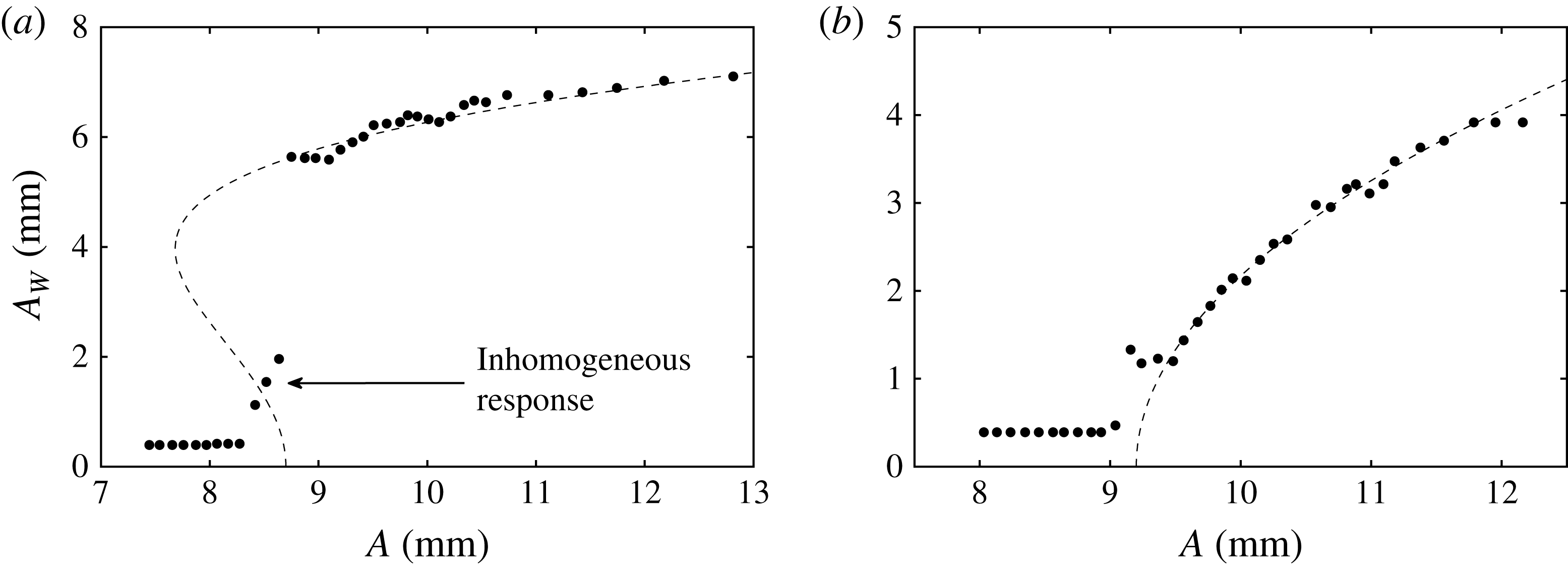
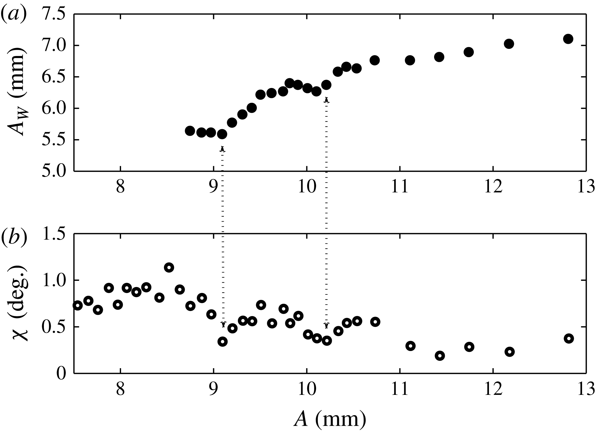
While the onset is not significantly altered by two-frequency excitation, this is not true of the nonlinear response. Figure 19(a,b) presents the fixed-frequency saturated wave response for
 ${\it\omega}=2.45$
and 2.55 Hz,
 $3/2$
excitation, with average
 ${\it\chi}=52.4$
and 51.9°, respectively. The responses exhibit the same transition from subcritical to supercritical bifurcation as seen in single-frequency excitation. However, as presented, there is a noticeable scatter in the data, contrasting the ordered single-frequency responses of figure 16(a,b). The scatter arises from the measurement, which was made by sampling a single crest of the saturated wave. This can be visualized by a time series of the central
 $(0,1)$
mode deflection, presented in figure 20 (parametric conditions marked in figure 18). The response is sampled for two periods of an
 $f=2.55~\text{Hz}$
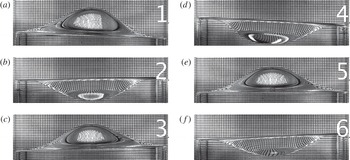
excitation at an amplitude near the onset such that the response remains regular. Inspection of the crests (labelled 1, 2 and 3) reveals that the wave is not periodic from crest to crest as was observed for a similar single-frequency excitation in figure 17. In contrast, here both the maximum wave amplitudes and reflection patterns vary from crest to crest. Addition of the
 $2{\it\omega}$
component breaks the subharmonic periodicity of the
 $(0,1)$
mode with the primary
 $3{\it\omega}$
component and the resulting wave is instead periodic with respect to the basic frequency,
 ${\it\omega}$
. We suspect that
 ${\it\phi}$
contributes to the observed crest-to-crest fluctuations, but this was not studied.
Images taken from two cell periods (
 $2T=4{\rm\pi}/{\it\omega}$
) of the simultaneous excitation of a
 $(0,1)$
and a
 $(1,1)$
mode with
 $[l/m,f,A,{\it\chi}]=[3/2,2.55~\text{Hz},1.40~\text{mm},48.0^{\circ }]$
. These images of the maximum
 $(0,1)$
wave deflections are taken at an interval
 $T/3$
and highlight its subharmonic periodicity with respect to the
 $3{\it\omega}$
excitation. The central deflections of these images are labelled on the time series data of figure 23. Also see supplementary movie 1.

Images taken from the same two-mode excitation as figure 21. These images of the maximum
 $(1,1)$
wave deflections are taken at an interval
 $T/2$
and highlight its subharmonic periodicity with respect to the
 $2{\it\omega}$
excitation. The
 $(1,1)$
component of the wave is parallel to the single-headed arrows drawn in panels (a) and (b). The sidewall deflection time series of figure 23 is built from data marked by the two-headed arrow of panel (a).

8.2. Multi-mode subharmonic
$3/2$
excitation

To illustrate a unique aspect of the two-frequency single-mode system, we present images and time series of a two-mode nonlinear response in figures 21–23. Also see supplementary movie 1 available at http://dx.doi.org/10.1017/jfm.2014.724. The images and data have been collected from the saturated response for two periods of a
 $3/2$
excitation with
 $f=2.55~\text{Hz}$
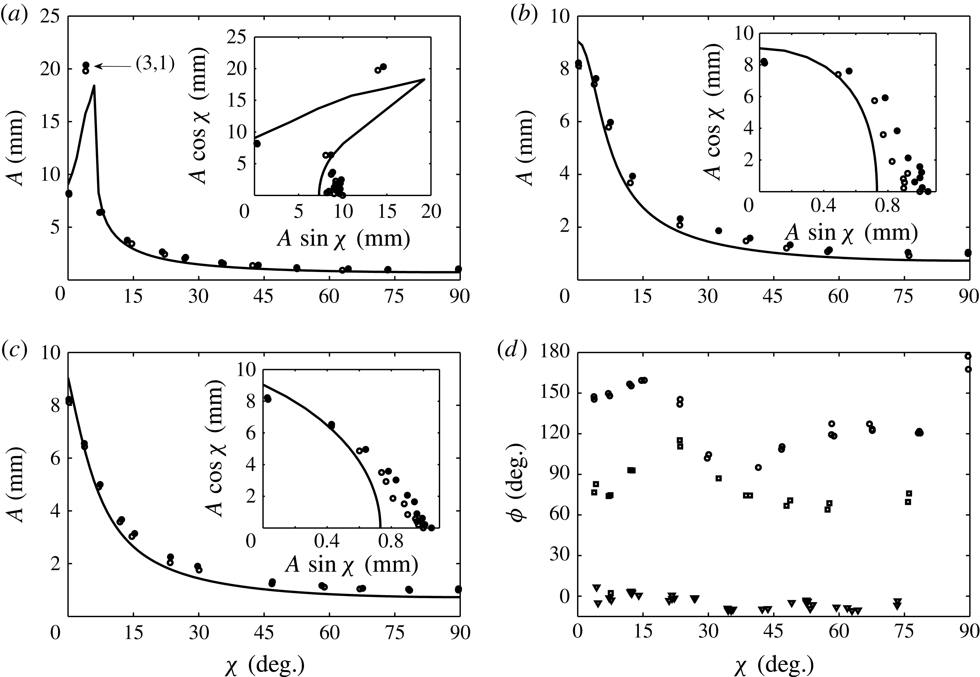
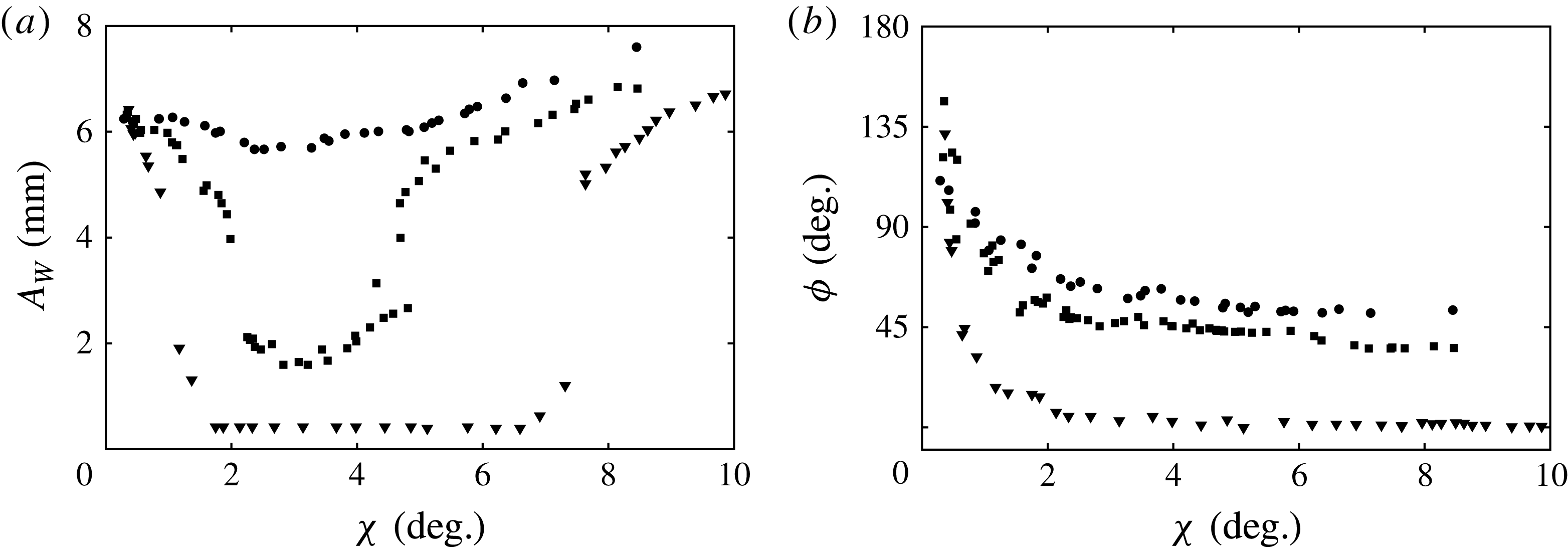
and
 ${\it\chi}=48.0^{\circ }$
, conditions near those of figure 20. This excitation was performed at a higher amplitude such that a
 $(1,1)$
mode (see figure 4) was excited by the
 $2{\it\omega}$
component, in addition to the
 $3{\it\omega}$
excitation of the
 $(0,1)$
mode.

The images of figures 21 and 22 have been selected to highlight the different periodicities of the
 $(0,1)$
and
 $(1,1)$
components of this wave. The times during the excitation at which both sets of images are taken are denoted by the numbered slices in the time series data. The images of figure 21, taken at an interval of
 $T/3$
, depict the maximum deflections of the
 $(0,1)$
mode component of the wave. The images of figure 22 were taken at an interval of
 $T/2$
in order to highlight the maximum deflections of the
 $(1,1)$
mode of the excitation. The arrow in images 7 and 8 is drawn parallel to this component. Time series data for the interface motion along the cell sidewall are also presented (bottom, figure 23) by taking data from the far left of the cell images, viz. the double arrow in image 7. It is evident that an
 ${\it\omega}$
modulation by the
 $(1,1)$
mode appears on top of the
 $3{\it\omega}/2$
response due to the
 $(0,1)$
mode. In contrast, the
 ${\it\omega}$
modulation is not noticeable in the time series of the central deflection (top, figure 23), which is suggested by the linear spatial form of the
 $(1,1)$
mode.
In summary, this excitation produces a wave whose
 $(0,1)$
and
 $(1,1)$
components execute three and two oscillations, respectively, over two periods of the basic frequency
 ${\it\omega}$
. It is similar to excitations used to create superlattice patterns in the high-frequency experiment; however, here only two linearly unstable modes participate instead of two continuous bands of wavenumbers (cf. Kudrolli, Pier & Gollub Reference Kudrolli, Pier and Gollub1998). Multi-mode waves are also possible in the discretized regime when only a single frequency is used, under the condition that the participating modes are close in wavenumber. This constraint is relaxed in two-frequency excitation, where any two modes can be simultaneously excited by correct tuning of the frequency ratio.
8.3. The
$3/4$
subharmonic excitation of the
$(0,1)$
mode


We have just considered a case where the
 $(0,1)$
mode is primarily excited by a
 $3{\it\omega}$
frequency, and is modified by a slower
 $2{\it\omega}$
frequency. To reveal potential behaviour when the modifying frequency is faster, we present results of the
 $(0,1)$
mode onset and bifurcation for
 $l/m=3/4$
with an average
 ${\it\chi}=23.1^{\circ }$
in figure 24. Little difference is found, as model agreement for the variable frequency and variable
 ${\it\chi}$
onsets in figure 24(a,b) is quite similar to what was seen for
 $3/2$
excitation in figure 18(a,b). Again,
 ${\it\phi}$
was not observed to have any effect on either the calculated curves or the experimental onsets. The
 $(0,1)$
mode bifurcation in figure 25(a,b) shows the same scatter as was observed for
 $3/2$
excitation. The crest-to-crest variance of the time series data of figure 26 supports the same explanation. Hence, within the scope of the experimental study, we do not find a difference between the addition of a greater or lesser second frequency.
Comparison between the experiment and the model for
 $l/m=3/4$
excitation for (a) average
 ${\it\chi}=23.1^{\circ }$
and (b) fixed
 $f=2.45~\text{Hz}$
. The experimental data points are defined as was done for figure 15.

Saturated wave response of the central
 $(0,1)$
mode deflection for
 $l/m=3/4$
excitation at (a) 2.45 Hz and (b) 2.55 Hz, as marked in figure 24. Parameters for the fit (7.1) are
 $[{\it\alpha},{\it\beta},A_{c}]=[-1.5\times 10^{-2},3.9\times 10^{-4},0.794]$
in (a) and
 $[1.1\times 10^{-2},0,0.74]$
in (b). Both fitting parameters
 $A_{c}$
are labelled on figure 24.

(a) Time series data for a
 $(0,1)$
mode excited with
 $[l/m,f,A,{\it\chi}]=[3/4,2.55~\text{Hz},1.10~\text{mm},26.9^{\circ }]$
and (b) the input parametric signal. Two periods of the
 $f=2.55~\text{Hz}$
excitation are depicted. These parametric conditions are marked by the star in figure 24.

8.4. The
$1/2$
harmonic excitation of the
$(0,1)$
mode


Finally, we turn to the study of harmonic excitation of the
 $(0,1)$
mode with
 $l/m=1/2$
. Here, as discussed in § 5.3, the mode for finite values of
 ${\it\chi}$
is simultaneously excited by both the
 ${\it\omega}$
and
 $2{\it\omega}$
components. The most dramatic aspect of this excitation is that the phase
 ${\it\phi}$
can significantly alter the
 $(0,1)$
mode threshold or suppress the mode entirely (see figure 8). Before confirming this prediction, we first review the experimental onset of single-frequency excitation of the
 $(0,1)_{h}$
mode in figure 27, and its bifurcation in figure 28. It was observed by Batson et al. (Reference Batson, Zoueshtiagh and Narayanan2013) that the instability appeared early for this mode, which was explained as the interaction between the harmonic meniscus waves and the harmonic excitation of the instability. The outcome of this interaction is that the
 $(0,1)_{h}$
mode is the only mode in the single-frequency experiment whose onset lies below the model prediction. Three data points in figure 28(a) exhibit a finite inhomogeneous deflection before the subcritical jump to Faraday resonance. This erroneous detection of resonance is indicative of the inhomogeneous excitation, which is not observed in any of the
 $(0,1)_{sh}$
bifurcation data.
Comparison between the experiment and the model for single-frequency harmonic excitation of the
 $(0,1)$
mode.





The fluctuations in the Faraday response of figure 28(a,b) are a separate phenomenon unique to harmonic excitation of the
 $(0,1)$
mode. Recalling that stray components can enter into the parametric signal produced by the shaker, figure 29 treats the intended single-frequency signal as a
 $l/m=1/2$
signal, and juxtaposes the resulting values of
 ${\it\chi}$
against a zoom of the wave response in figure 28(a). Here it appears that fluctuations in the wave response correspond to those in the angle
 ${\it\chi}$
, most apparent at excitation amplitudes of 9.2 and 10.2 mm. This kind of interaction was not observed in the single-frequency wave response for the subharmonic
 $(0,1)$
mode (see figure 16), where undesired signal harmonics were also present. These are the only results we report that exhibit a high sensitivity to stray frequencies in the parametric input, and, along with the phase dependence highlighted by the model predictions, motivate us to further study this
 $1/2$
excitation.
Juxtaposition of the wave response of figure 27 with the angle
 ${\it\chi}$
. The parametric signals producing the response data, intended to contain only a single frequency, inevitably contain undesired harmonics, and the values of
 ${\it\chi}$
have been calculated using the
 $2{\it\omega}$
content in each signal.

Figure 30(a–c) compares experimental onset data with the predictions that were initially given in figure 8. Up to this point, phase has not been observed to affect the onset behaviour for either
 $l/m=3/2$
or
 $3/4$
excitation. The phases for these input signals have been calculated by Fourier analysis and are presented in figure 30(d). Although the phases clearly fluctuate about the set points 0°, 90° and 135°, they show the desired trends when moving from one data set to another, especially at low values of
 ${\it\chi}$
, where the phase average is 0, 90 and 135°, respectively. As a guide, the model predictions have been calculated using these averages for each figure. The threshold data at
 ${\it\chi}=0$
for each figure are identical, as expected. Inspecting the first unstable point for a finite
 ${\it\chi}$
in each figure, the calculated
 ${\it\phi}$
for these signals increases from 6.6° in figure 30(a) to 82.8° in figure 30(b) and then to 147.4° in figure 30(c). The associated threshold amplitudes decrease, in accordance with the model predictions, where the upper point in figure 30(a) excites the
 $(3,1)$
mode as predicted. To map more precisely this region where the divergence in the onset occurs, the saturated response is presented in figure 31(a) for a fixed amplitude
 $A$
for values of
 ${\it\chi}$
where the gap occurs. The amplitude for these data was exceptional and held between 9.8 and 9.9 mm, and the phases are given in figure 31(b). Both figures clearly show that parametric resonance is restored as the phase of the
 $2{\it\omega}$
component is increased.
Comparison between the experiment and the model for
 $l/m=1/2$
excitation at a fixed frequency of 3.6 Hz for average
 ${\it\phi}$
of (a) 0°, (b) 90° and (c) 135°. (d) The actual phases for the signals in each data set. The
 $(0,1)$
mode was excited for all these data, except for the point at
 ${\it\chi}=4.1^{\circ }$
and
 $A=20.4~\text{mm}$
in (a), where the
 $(3,1)$
mode was excited.

Saturated wave response of the
 $(0,1)_{h}$
mode for
 $1/2$
excitation, where measurements were taken for a fixed frequency of 3.6 Hz, amplitude
 $A$
of 10 mm, for input
 ${\it\phi}$
of 0, 45 and 90°. The calculated values of
 ${\it\phi}$
for the signals producing the data in (a) are given in (b).

9. Conclusion and discussion
This work on two-frequency excitation of single-mode Faraday waves follows the initial design of a small-cylinder experiment by Batson et al. (Reference Batson, Zoueshtiagh and Narayanan2013), whose purpose was to verify the linear theory of Kumar & Tuckerman (Reference Kumar and Tuckerman1994). This theory, written for horizontally infinite viscous layers, was extended to the case of finite cells in Batson et al. (Reference Batson, Zoueshtiagh and Narayanan2013) by application of a sidewall stress-free boundary condition. By judicious choice of the system fluids, sidewall and interfacial dissipation were rendered negligible compared to that of the bulk domain, and good agreement between the thresholds of instability was found without inclusion of phenomenological parameters.
The current study extends the work of Batson et al. (Reference Batson, Zoueshtiagh and Narayanan2013) to the case of two-frequency excitation, which had yet to be studied for low-frequency excitation in small cells where modes are highly discretized. Here we extend the finite cell theory to two-frequency excitation and use it as a guide to explore this regime. Specifically, the investigation focuses on cases where the ratio of the two frequencies is of the order of one, and we find that experimental agreement with the two-frequency theory is qualitatively the same as seen for single-frequency excitation. A frequency ratio in which the phase difference,
 ${\it\phi}$
, has a significant influence on the instability onset is also predicted and verified with the experiment. Further experimental data of the saturated wave response have been used to compare the nonlinear response of the single- and two-frequency cases. The harmonic content of each imposed vibrational signal has been measured with Fourier analysis.
In the context of two-frequency excitation, an interesting avenue of future investigation is the interaction between the instability and the meniscus waves. This interaction, which is most noticeable when the
 $(0,1)$
mode is excited harmonically, can result in detection of the instability below the model prediction, as was shown in figure 27. Close inspection of the onsets in figure 30(b,c), where the
 $(0,1)$
mode is harmonically excited by the
 ${\it\omega}$
component and subharmonically by the
 $2{\it\omega}$
component, also suggests that there exist finite values of
 ${\it\chi}$
where this interaction is broken and early detection is no longer observed. An inhomogeneity can be shown to cause a jump to the parametric solution in a nonlinear oscillator. This ‘jump’ has been shown analytically by HaQuang, Mook & Plaut (Reference HaQuang, Mook and Plaut1987), who considered a single-degree-of-freedom oscillator driven by both parametric and forced excitations. They used a perturbation method of multiple scales to calculate the oscillator nonlinear response, and show that the inhomogeneous response joins with the parametric response at a threshold parametric amplitude. Alternatively, their calculation can also show that increase of the inhomogeneity amplitude for fixed parametric amplitude effects the same jump. This work was extended by Plaut, Gentry & Mook (Reference Plaut, Gentry and Mook1990) to the case of multiple parametric and inhomogeneous excitations, and they showed that there are many potential resonances between these excitations.
Two-frequency excitation presents an opportunity to study novel multi-mode interactions, particularly those near codimension-two points where the participating modes are primarily excited by the
 $l{\it\omega}$
and
 $m{\it\omega}$
components, as in figures 21–23. Such experiments would be reminiscent of Ciliberto & Gollub (Reference Ciliberto and Gollub1985), who studied nonlinear competition between
 $(4,3)$
and
 $(7,2)$
modes in a small-cylinder single-frequency Faraday experiment. They reported parameter spaces in which the two-mode response undergoes both periodic and chaotic amplitude modulations. These states, in addition to azimuthal rotation and quasi-periodic amplitude modulations, were predicted by the detailed theory of Crawford et al. (Reference Crawford, Knobloch and Riecke1990). Less detailed theories were proposed by Meron & Procaccia (Reference Meron and Procaccia1986) and Umeki & Kambe (Reference Umeki and Kambe1989) and could serve as a better starting point to describe interaction in the two-frequency experiment. Such a two-frequency experiment would be an ideal candidate to employ modern interface-tracking methods (see e.g. Cobelli et al.
Reference Cobelli, Maurel, Pagneux and Petitjeans2009; Moisy, Rabaud & Salsac Reference Moisy, Rabaud and Salsac2009).
Acknowledgements
W.B. and R.N. acknowledge support from NASA NNX11AC16G, and from NSF 0968313 and 1402151. F.Z. acknowledges support from CNRS-CNES, ESA and a Marie Curie International Research Staff Exchange Scheme Fellowship within the 7th European Community Framework Programme.
Supplementary movie
Supplementary movie is available at http://dx.doi.org/10.1017/jfm.2014.724.