Abbreviations

EEEnd-Effector

MMFMultimodal Fusion

FPNFeature Pyramid Network

RPNRegion Proposal Network

mAPMean Average Precision

FCNFully Connected Network

ROIRegions of Interest

DGADepth-Guided Attention

IoUIntersection over Union

CLSCurriculum Learning Strategy

FWFixed Weights

DDEDynamic Depth Estimation

SDStandard Deviation

MAEMean Absolute Error

FOVField of View

PDProportional-Derivative

TSRTask Success Rate

2. Multimodal learning Mask R-CNN

2.1. RGB-D multimodal fusion module

This network utilizes RGB-D multimodal fusion module (MMF) input to achieve heterogeneous feature extraction through parallel data streams. The RGB image stream receives 8-bit color data at a resolution of 1,280 × 720 × 3, processed through pixel-level normalization, as shown in Eq. (1):

(1) \begin{equation}\boldsymbol{{I}}_{\text{norm}}=\frac{\boldsymbol{{I}}_{\textrm{raw}}}{255}\end{equation}

where I _norm represents the normalized image, while I _raw is the original image, mapped to the range of [0,1]. The depth image stream processes 1,280 × 720 depth data in Z16 format, with the depth value intercepted in the range of [0, 2000] and then normalized, as shown in Eq. (2):

(2) \begin{equation}\boldsymbol{{D}}_{\text{norm}}=2\cdot \frac{\boldsymbol{{D}}_{\textrm{raw}}}{2000}-1\end{equation}

where D _norm represents the normalized depth image, and D _raw is the original depth image. This generates a normalized tensor aligned with the RGB modality, which is then normalized to the range of [−1, 1] using min–max scaling. This preprocessing strategy effectively eliminates noise from the depth sensor while preserving millimeter-level geometric accuracy.

The network has designed a hierarchical feature fusion mechanism, as depicted in Figure 1. Both streams utilize an improved ResNet50-FPN backbone network with shared parameters, which includes:

1. 1. Shallow feature sharing: Weight sharing between Conv1-Conv3 layers to extract common edge and texture features.

2. 2. Deep modality differentiation: Conv4-Conv5 layers differentiate into dedicated paths for RGB and depth, respectively, extracting color semantics and geometric structure features.

3. 3. Multi-scale fusion: At the P3-P5 levels of the feature pyramid network (FPN) output, feature fusion is achieved through adaptive channel alignment and element-wise summation, as follows in Eq. (3):

(3) \begin{equation}\boldsymbol{{F}}_{\text{fusion}}^{i}={\textrm{Conv}}_{1\times 1}\left(\boldsymbol{{F}}_{\text{color}}^{i}\right)+{\textrm{Conv}}_{1\times 1}\left(\boldsymbol{{F}}_{\text{depth}}^{i}\right) \left(i\in \left\{3,4,5\right\}\right)\end{equation}

where $\boldsymbol{{F}}_{\text{fusion}}^{i}$ represents the fused feature map of the layer i, $\boldsymbol{{F}}_{\text{color}}^{i}$ denotes the feature map extracted from the RGB modality at the layer i, and $\boldsymbol{{F}}_{\text{depth}}^{i}$ denotes the feature map extracted from the depth modality at the layer i.

The 1×1 convolutional layer is used to unify the channel dimension (256→256), and the fused feature tensor is input into the subsequent region proposal network (RPN). This design significantly enhances the representation capability for occluded and reflective objects while reducing the number of parameters, as detailed in Table I.

Table I.

Ablation study on MMF module (mAP@0.5).

Figure 1.

MMF input preprocessing, (a) hierarchical feature fusion, (b) structure of the MMF module.

This layered fusion strategy retains spatial details at lower levels while integrating semantic context at higher levels. The output size of the fusion module is 14×14×256, and classification and bounding box regression are performed subsequently through the fully connected network (FCN). Additionally, a Softmax layer is used for the final class prediction.

Figure 2.

Mask R-CNN network architecture based on RGB-D multimodal learning.

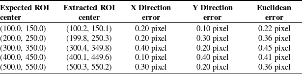
The network retains the architecture of Mask R-CNN and has made key improvements for robotic grasping scenarios, as shown in Figure 2: the RPN uses five anchor scales of {32, 64, 128, 256, 512} and three aspect ratios of 0.5, 1, and 2 to optimize the prior box distribution for robotic tasks; the regions of interest (ROI) align layer extracts 7 × 7 region features from the fused feature map, with a coordinate alignment error of less than 0.5 pixel, as detailed in Table II; the dual-task head consists of a classification-box regression head (Faster R-CNN) and a mask prediction head, which operate in parallel, with the latter incorporating a depth-guided attention mechanism, as discussed in Section 2.2.

Table II.

Coordinate alignment error experiment.

The total number of parameters in the network is 46.3 million, which is an increase of only 4.8% compared to the baseline model.

2.2. Depth-guided attention module

In the Delta robot grasping task, the material of the target objects (such as metal and glass) and complex scenes (such as occlusion and reflection) pose significant challenges to mask prediction accuracy. The mask head of the traditional Mask R-CNN only relies on RGB features, which makes it difficult to effectively distinguish objects with similar geometry but different materials. To address this, this paper designs the depth-guided attention mechanism (DGA), which dynamically integrates information from the depth modality to enhance the robustness of mask predictions. The core idea can be expressed as Eq. (4):

(4) \begin{equation}\boldsymbol{{A}}_{\textrm{att}}=\sigma \!\left(\boldsymbol{{W}}_{\!a}\cdot \left[\boldsymbol{{F}}_{\text{fusion}};\,\boldsymbol{{F}}_{\text{depth}}\right]\right)\odot \boldsymbol{{F}}_{\text{fusion}}\end{equation}

where A _att represents the attention weight matrix, σ denotes the Sigmoid activation function, W _a is the learnable weight parameter, [ $\cdot\,;\,\cdot$ ] indicates channel concatenation, and ⊙ signifies element-wise multiplication. This mechanism adaptively weights the fused features in both spatial and channel dimensions using deep features.

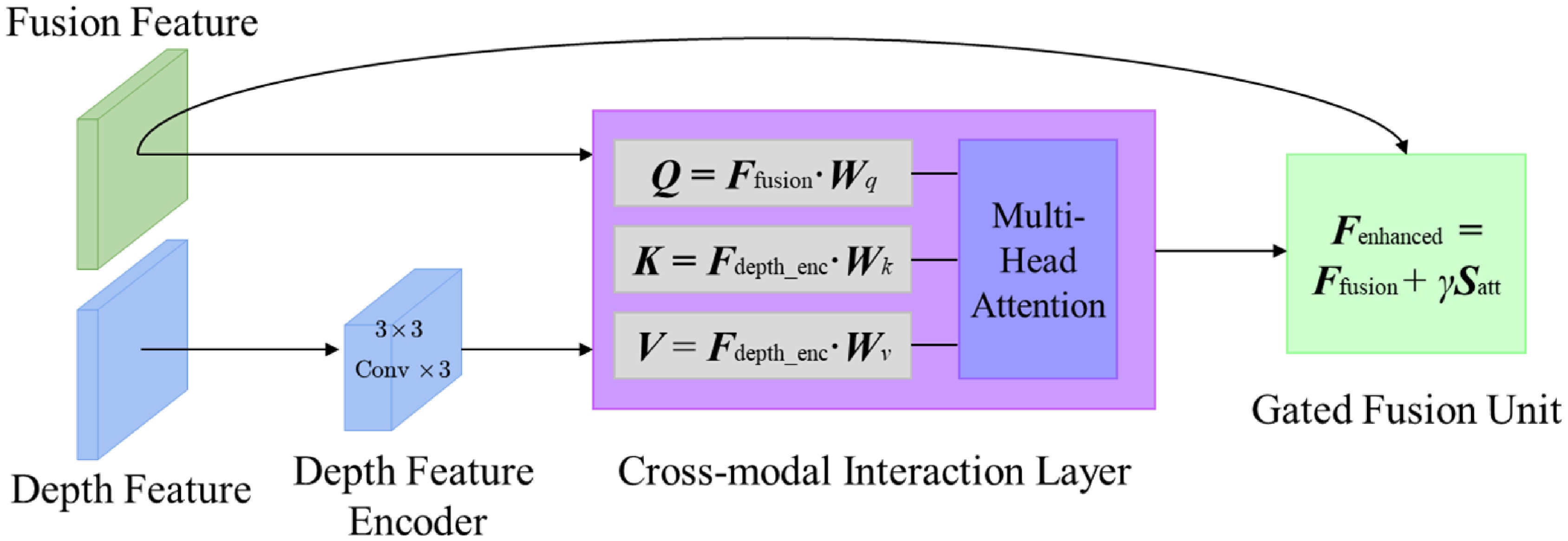
The DGA module consists of a deep feature encoder, a cross-modal interaction layer, and a gated fusion unit submodule, as shown in Figure 3. The deep feature encoder encodes the depth features F _depth output by the FPN into a tensor with the same resolution as the fused features through three layers of 3 × 3 convolution. The cross-modal interaction layer computes the correlation between the fused features and the depth features using cross-attention, as follows in Eqs. (5) and (6):

Figure 3.

DGA module.

(5) \begin{align} \boldsymbol{{Q}}=\boldsymbol{{F}}_{\text{fusion}}\boldsymbol{{W}}_{q}, &\quad\!\! \boldsymbol{{K}}=\boldsymbol{{F}}_{\text{depth}}\boldsymbol{{W}}_{k},\quad \boldsymbol{{V}}=\boldsymbol{{F}}_{\text{depth}}\boldsymbol{{W}}_{v} \end{align}

(6) \begin{align} \boldsymbol{{S}}_{\textrm{att}} &=\text{Softmax}\!\left(\frac{\boldsymbol{{Q}}\boldsymbol{{K}}^{T}}{\sqrt{d_{k}}}\right)\boldsymbol{{V}} \end{align}

where W _q , W _k , and W _v represent the learnable weight parameters for Q , K , and V , respectively, while S _att denotes the attention map. The gated fusion unit further integrates the attention map S _att with the original fused features, using Eq. (7):

(7) \begin{equation}\boldsymbol{{F}}_{\text{enhanced}}=\boldsymbol{{F}}_{\text{fusion}}+\gamma \cdot \boldsymbol{{S}}_{\textrm{att}}\end{equation}

where γ is a learnable scaling factor, with an initial value of 0.1.

Ablation experiments on the synthetic dataset indicate that the DGA module significantly enhances segmentation accuracy in complex scenarios, as detailed in Table III.

Table III.

Ablation study on DGA module (IoU).

To meet the real-time requirements of the Delta robot, the DGA module employs a lightweight design: channel compression reduces the number of attention channels from 256 to 64, with only a 0.8% loss in accuracy; sparse computation applies the DGA only at the P4 level of the FPN, resulting in a 22% increase in inference speed. On the Advantech EPC-P3086 industrial computer platform, the inference time for the mask prediction head that includes the DGA is 8.3 ms.

2.3. Fine tuning

To enhance the task adaptability of Mask R-CNN under multimodal inputs, this section employs a fine-tuning framework based on category reduction and domain adaptation. It reduces the 80 target categories from general scenes to 4 target categories specific to industrial scenarios, optimizing model parameters for dynamic grasping scenarios involving Delta robots. The tuning process combines the characteristics of the MMF module and the DGA module and realizes the migration of the model from general scenarios to industrial scenarios through a hierarchical parameter optimization strategy.

Using the Mask R-CNN pre-trained on the COCO dataset as the base model retains its general feature extraction capabilities. For four types of targets in industrial scenarios: PLA plastic workpieces, metal workpieces, glass workpieces, and EE, as shown in Figure 4. Remap the classification head by replacing the 80-class classification head of COCO with a 4-class classification head. The parameters of the MMF module and the DGA module are randomly initialized to avoid feature bias caused by modal differences.

Figure 4.

Workpieces, (a) plastic workpiece, (b) metal workpiece, (c) glass workpiece, (d) EE.

Utilizing a layered parameter unfreezing mechanism to freeze the backbone network, the weights of the Conv1-Conv3 layers in ResNet50-FPN are fixed, preserving the ability to extract low-level edge and texture features. Modality-specific layer tuning is conducted, unfreezing the RGB and depth branch parameters in the Conv4-Conv5 layers to enhance the adaptability of the model to multimodal features in industrial scenarios. During the dynamic training of the DGA module, the cross-modal interaction layer and the gated fusion unit are actively involved throughout the training process, achieving adaptive fusion of geometric and semantic features through end-to-end learning.

In addition, to address variations in lighting conditions and sensor noise in industrial environments, a joint enhancement of 12,000 pairs of labeled RGB-D images was performed, as shown in Figure 5. First, geometric perturbations were applied, introducing random rotations within a ± 15° range, scaling between 0.8 and 1.2 times, and affine transformations to both the RGB and depth images. Next, modality-specific noise was added, with Gaussian noise of σ _G = 0.05 introduced to the RGB channel, along with color disturbances of ΔH = ±0.1 and ΔS = ±0.3; the depth channel received simulated impulse noise at a density of 5% and bilateral filtering for denoising, enhancing the robustness of the model against anomalies in depth sensors. Finally, synthetic occlusions were added, randomly inserting occlusion samples covering 15–25% of the area in 20% of the training batches to improve the attention focusing capability of the DGA module.

Figure 5.

Data augmentation, (a) geometric perturbation, (top) 10° counterclockwise and 15° clockwise rotation, and (bottom) affine transformation, (b) synthetic occlusion, (top) occlusion 15%, and (bottom) occlusion 30%, (c) modality-specific noise, (top left) σ_G = 0.05 ΔH = −0.1, (top right) σ_G = 0.05 ΔS = 0.3, (bottom left) 5% pulse noise, and (bottom right) bilateral filtering.

2.4. Training

For this network model, optimize the loss function and define a multi-task joint loss function, as follows in Eq. (8):

(8) \begin{equation}\mathcal{L}_{\text{total}}=\lambda _{1}\mathcal{L}_{\textrm{cls}}+\lambda _{2}\mathcal{L}_{\textrm{box}}+\lambda _{3}\mathcal{L}_{\text{mask}}+\lambda _{4}\mathcal{L}_{\textrm{dga}}\end{equation}

where $\mathcal{L}_{\textrm{cls}}, \mathcal{L}_{\textrm{box}}, \mathcal{L}_{\textrm{mask}}$ are the classification loss, bounding box regression loss, and mask segmentation loss, respectively, and $\mathcal{L}_{\textrm{dga}}$ is the attention supervision loss, as follows in Eq. (9):

(9) \begin{equation}\mathcal{L}_{\textrm{dga}}=||\boldsymbol{{S}}_{\textrm{att}}-\boldsymbol{{Y}}_{\text{edge}}||_{2}\end{equation}

where $\boldsymbol{{Y}}_{\text{edge}}$ is the object edges extracted from the depth map using the Canny operator as prior knowledge. The weight coefficients λ ₁ to λ ₄ adopt a curriculum learning strategy (CLS), as follows in Eq. (10):

(10) \begin{equation}\lambda _{i}\left(t\right)=\lambda _{i}^{\text{start}}+\left(\lambda _{i}^{\textrm{end}}-\lambda _{i}^{\text{start}}\right)\!\cdot \frac{t}{T}\end{equation}

where the initial weights are denoted as $\lambda _{i}^{\text{start}}$ and the final weights as $\lambda _{i}^{\text{end}}$ , with initial values of [1.0, 1.0, 0.5, 0.2]. These values are linearly adjusted over the training epochs to [0.8, 0.8, 1.0, 0.5] to balance the convergence speed of each task. The classification loss λ ₁ and localization loss λ ₂ decrease from 1.0 to 0.8 to reduce reliance on the foundational tasks, while the segmentation loss λ ₃ increases from 0.5 to 1.0 to enhance attention to mask details. The attention supervision loss λ ₄ rises from 0.2 to 0.5 to guide the model in learning geometric features in the later stages. For further details, see Table IV.

Table IV.

Curriculum learning strategy.

The CLS reduces the number of training iterations by 17%, as adjustments to task weights prevent early oscillations. The intersection over union (IoU) for the target object improves by 4.8%, demonstrating the effectiveness of the enhanced attention mechanism in the later stages. This approach avoids conflicts driven by tasks, allowing early high-weight classification and localization tasks to converge quickly, thereby providing reliable candidate ROI for subsequent segmentation and preventing mask predictions from failing due to localization errors. It alleviates optimization imbalances; if weights are fixed throughout (e.g., λ ₃ = 1.0), complex tasks may interfere with foundational tasks due to excessively large gradient magnitudes. The phased adjustments enable a smoother transition, enhancing overall convergence. The effectiveness of the attention mechanism is strengthened, as increasing λ ₄ in the later stages compels the model to refine segmentation edges using deep geometric information once the foundational tasks stabilize, such as the reflective areas of metal workpieces and the translucent areas of glass workpieces.

A custom dataset containing 12,000 pairs of RGB-D images, including workpieces such as PLA plastic, metal, and glass materials, is used for training and validation. The multimodal learning-based model in this paper achieves 95.2% mAP@0.5 and 87% IoU, exceeding the baseline model 84.7% mAP@0.5 and 73% IoU, exceeding the late feature fusion model 87.1% mAP@0.5 and the spatial attention model 80% IoU, respectively. As shown in Figures 6(a) and 7(a), the training curve demonstrates rapid convergence. The designed method achieves 90% mAP@0.5 and 80% IoU within 40 epochs. The performance comparison of the MMF module and the DGA module designed in this paper with other methods under fixed weights (FW) and CLS approaches are shown in Figures 6(b) and 7(b).

Figure 6.

The MMF module, (a) training curve, (b) performance comparison.

Figure 7.

The DGA module, (a) training curve, (b) performance comparison.

The model achieves a real-time inference speed of approximately 50 FPS on the Advantech EPC-P3086 industrial computer platform, ensuring that visual information can be processed and fed back in about 20 milliseconds.

3. Dynamic depth estimation

In the depth images generated by the Intel RealSense D455, there are also some common and significant issues, which can be summarized in the following two aspects:

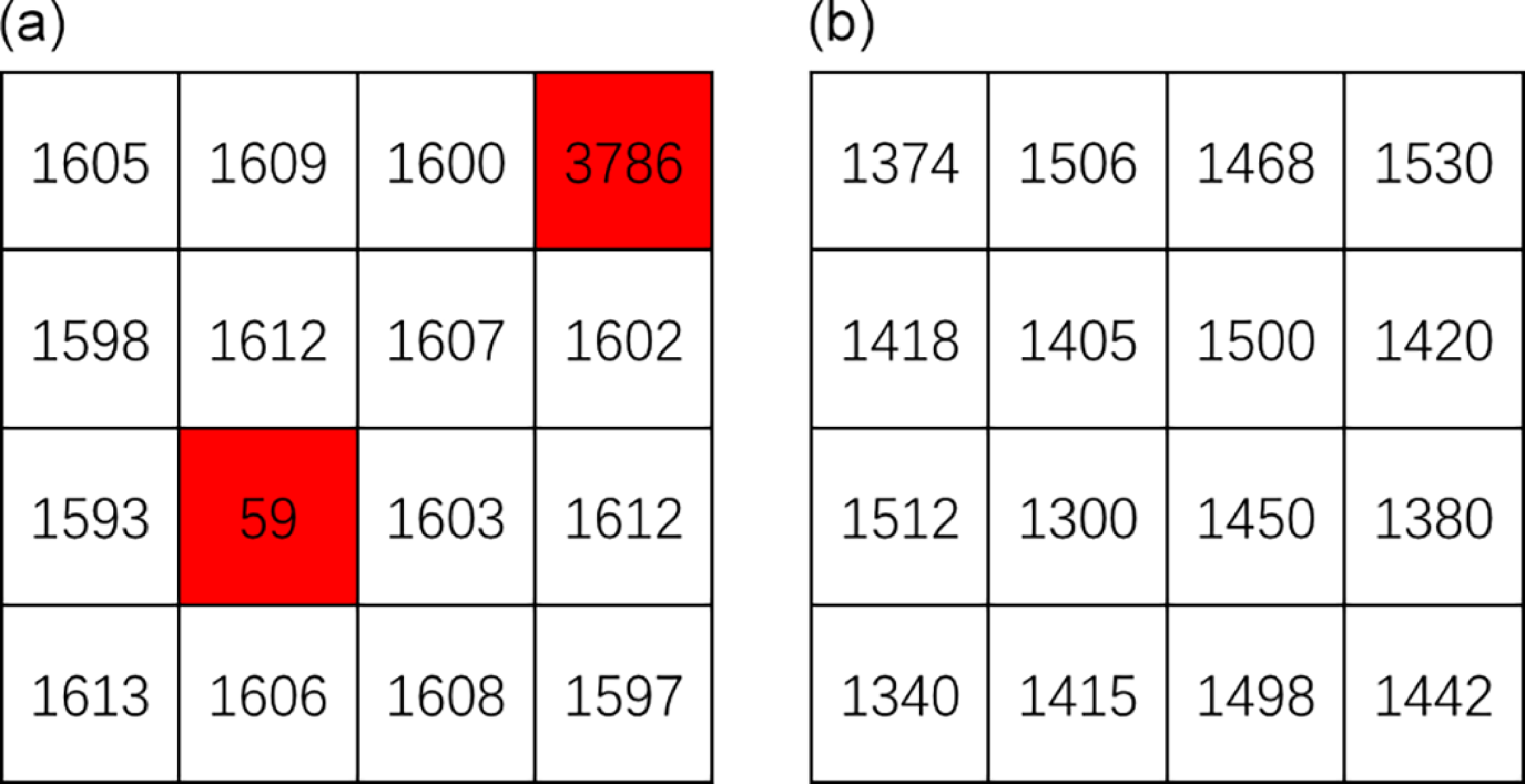
One is that the depth image contains erroneous pixel values that cannot accurately represent depth. For example, the pixel segment in the depth image shown in Figure 8(a) corresponds to an object at a depth of 1600 mm, and the values of the erroneous pixels (marked in red) differ significantly from the actual depth of the object.

Figure 8.

Common issues with depth images, (a) local outlier, (b) depth fluctuation.

The other is that the depth values of the same object in the depth image are different and fluctuate. For example, the pixel segment is shown in Figure 8(b). These pixels correspond to a plane object with a depth of 1,400 mm. The pixel segment shows that the pixels on the same plane fluctuate by about 150 mm.

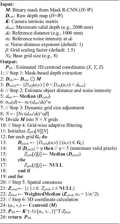
In order to solve the above problems, the following dynamic depth estimation (DDE) algorithm is designed, see Algorithm 1 for details. The main idea of the algorithm is: first take the instance segmentation mask in the depth image and divide it into n grid cells; then calculate the local depth Z _grid of each grid cell to eliminate local outliers; then weight these local depths by inverse variance to obtain Z _cand to suppress depth fluctuations; finally, concatenate the target mask centroid (u _c , v _c ) and the object depth Z _final, and output the target three-dimensional coordinates P _3D through the camera model, see Section 4 for details.

Algorithm 1.

Dynamic Depth Estimation.

Considering that the noise intensity σ _int and the object distance d directly determine the statistical characteristics and reliability of depth data and are highly coupled with the physical model of the sensor, the influence of other variables (such as lighting and material) has been effectively isolated by the preliminary part of the model (MMF module, DGA module). This ensures the focus and efficiency of the depth estimation part; thus, the relationship between the two and the number of grid cells N is established.

The noise model of the depth sensor is usually Gaussian noise, and the noise intensity generally varies exponentially with the distance of the object from the sensor, as shown in Eq. (11):

(11) \begin{equation}\sigma _{int}(d)=\sigma _{0}\cdot \left(\frac{d}{d_{0}}\right)^{\alpha }\end{equation}

where σ _int (d) is the noise intensity at the object distance d, σ ₀ is the reference noise intensity, d ₀ is the reference distance, which is generally the typical working distance of the sensor, and α is the relationship exponent, usually α ≈ 1. In general, the greater the noise, the more grid cells N are needed. By increasing the number of grid cells, multiple local depth values can be used to reduce the impact of noise and improve the accuracy of depth estimation, as shown in Eq. (12):

(12) \begin{equation}N(\sigma _{int})=\left[N_{0}\cdot \left(\frac{\sigma _{int}}{\sigma _{0}}\right)^{\beta }\right]\end{equation}

where N ₀ is the number of reference grid cells, $\beta$ is the adjustment factor used to control the relationship between noise intensity and the number of grid cells, usually within [Reference Zhu, Navarro-Alarcon, Passama and Cherubini1, Reference Lagneau, Krupa and Marchal2]. Substituting (11) into (12) can be expressed as Eq. (13):

(13) \begin{equation}N(d)=\left[N_{0}\cdot \left(\frac{d}{d_{0}}\right)^{\alpha \beta }\right]\end{equation}

This relationship implies that as the distance d of an object increases, the noise σ _int also increases, and the number of grid cells N correspondingly increases, thereby enhancing the stability and robustness of depth estimation.

When calculating the independent depth value of each grid cell, the minimum valid pixel threshold is set, and only when the number of valid pixels in the grid $\eta$ ≥ 5 is involved in the calculation, the interference of sparse data is avoided and adaptive filtering is realized. Through the spatial consensus mechanism, the local depth values of the valid grid cells are weighted by inverse variance.

Let the local depth values in the effective grid cell G _ij be Z _cand = {z ₁, z ₂, …, z _k }, with each value z _i corresponding to a variance of σ _i ², as follows in Eq. (14):

(14) \begin{equation}\sigma _{i}^{2}=\frac{1}{n_{i}-1}\sum _{\left(u,v\right)\in \boldsymbol{{G}}_{ij}}\left(D\!\left(u,v\right)-\mu _{i}\right)^{2}\end{equation}

where D(u,v) is the depth value in the grid cell G _ij , n _i is the number of valid pixels in it, and μ _i is the mean of the depth value in it, as follows in Eq. (15):

(15) \begin{equation}\mu _{i}=\frac{1}{n_{i}}\sum _{\left(u,v\right)\in \boldsymbol{{G}}_{ij}}D\!\left(u,v\right)\end{equation}

Sort Z _cand by the median z _i in ascending order to get the ordered sequence z ₍₁₎, z ₍₂₎, …, z _(k); calculate the cumulative weight for each median, as follows in Eq. (16):

(16) \begin{equation}W_{j}=\sum _{i=1}^{j}\omega _{\left(i\right)}\end{equation}

where ω _(i) is shown in Eq. (17):

(17) \begin{equation}\omega _{\left(i\right)}=\frac{1}{\sigma _{i}^{2}}\end{equation}

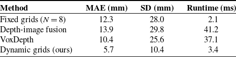
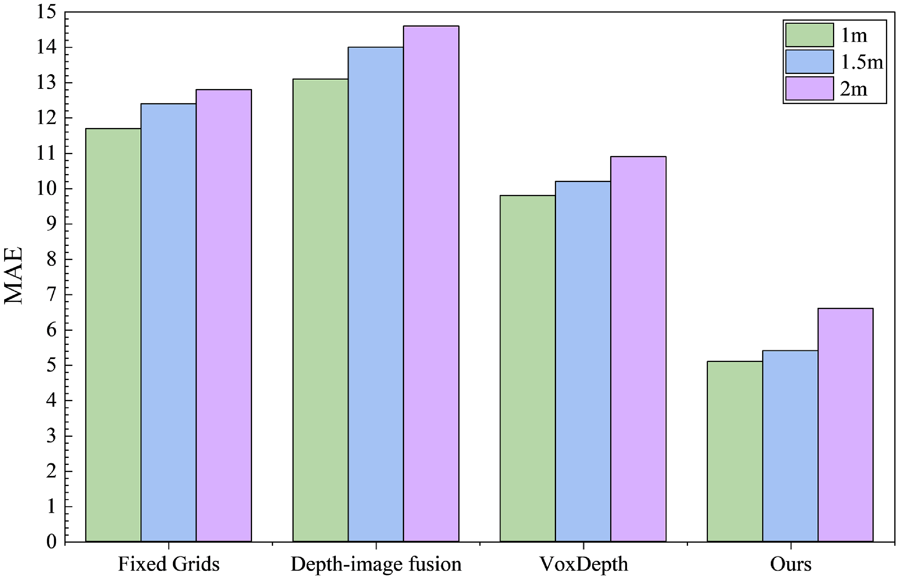
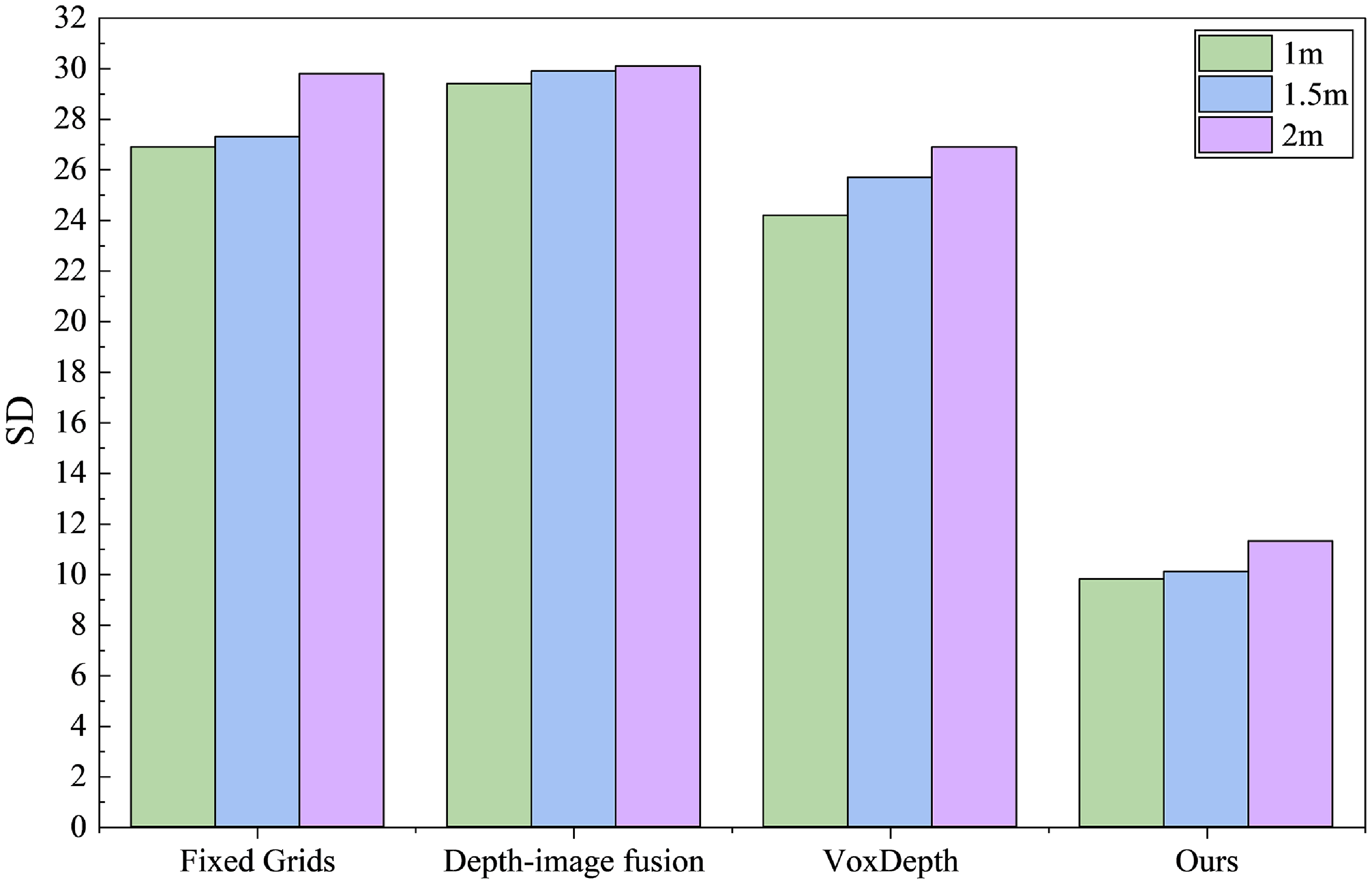
Find the minimum j that satisfies $W_j\geq 1/2W_k$ , to determine the median, then Z _final = z _{( j)}. The smaller the variance σ _i ², the more stable the depth value of the grid, the larger the weight ω _i , and the greater the contribution to the final result. By weighting the median, the influence of high-variance grids that are severely affected by noise on the final depth estimation is weakened, thereby suppressing depth fluctuations. The measurement area selected is shown in Figure 9. Compared with the fixed grid strategy, Perezyabov et al. [Reference Perezyabov, Gavrilenkov and Afanasyev22] Depth-image fusion method, and Chakrabarty et al. [Reference Chakrabarty, Dixit and Sarangi23] VoxDepth method, the designed method reduces the depth fluctuation error by 54, 59, and 45%, respectively. For a plastic workpiece at a distance of 1,500 mm, the standard deviation (SD) of the depth estimation decreases from ±28 mm with the fixed grid, ±29.8 mm with the Depth-image fusion method, and ±25.6 mm with the VoxDepth method to ±10.4 mm, as detailed in Table V. Furthermore, testing has shown that although the LiDAR-visual-inertial SLAM system integrating visual point-line features of Hui et al. [Reference Hui, Zhou and Liu24] and the optical flow-based stereo visual odometry of Liu et al. [Reference Liu and Zhou25] achieve high accuracy, their processing times are 168.3 ms and 90.9 ms, respectively, which do not meet the requirements for real-time performance. Depth estimation experiments were conducted at distances of 1, 1.5, and 2 m from the workpiece, respectively. The MAE and SD statistical indicators for the four methods are shown in Figures 10 and 11.

Table V.

Performance of regional depth estimation.

Figure 9.

Objects’ measured areas, (a) uneven surface, (b) object’s edge.

Figure 10.

MAE of depth estimation methods.

Figure 11.

SD of depth estimation methods.

Figure 12.

Mechanism schematic diagram of Delta robot.

4. Visual servo control

In order to facilitate the analysis of the motion rule of the robotic visual servo system, according to the research of Ni et al. [Reference Ni, Mei and Hu26], the kinematic model of the Delta robot is first established, and its mechanism is simplified to the structure shown in Figure 12. The dimensional parameters are detailed in Table VI.

Table VI.

Dimensional parameters of Delta robot.

As shown in Figure 12, the moving platform is simplified to a mass point $O^{\prime}$ , and the coordinate system O-xyz is established at the center of the static platform. In this coordinate system, the position vector r = (x y z)^T of the moving platform reference point $O^{\prime}$ can be expressed as Eq. (18):

(18) \begin{equation}\boldsymbol{{r}}=\boldsymbol{{e}}_{i}+l_{1}\boldsymbol{{u}}_{i}+l_{2}\boldsymbol{{w}}_{i}, \quad i=1,2,3\end{equation}

where the modulus of e _i = e(cos $\beta$ _i , sin $\beta$ _i , 0) (i = 1, 2, 3) represents the difference in radius of the circumcircle between the moving platform and the static platform, and in Figure 12, it indicates the vector from O to A _i ; $\beta$ _i represents the structural angle of the static platform, with $\beta$ _i = (i−1)2π/3 − π/6; l ₁, l ₂, u _i , and w _i represent the limb lengths and unit vectors of the active and passive limbs in branch i, respectively, and u _i is shown in Eq. (19):

(19) \begin{equation}\boldsymbol{{u}}_{i}=\left(\cos \beta _{i}\cos \theta _{i}\quad \sin \beta _{i}\cos \theta _{i}\quad {-}\!\sin \theta _{i}\right)^{\textrm{T}}\end{equation}

where θ _i represents the rotation angle of the active limb i (i = 1, 2, 3). By identity transformation, we get Eq. (20):

(20) \begin{equation}\boldsymbol{{w}}_{i}=\frac{1}{l_{2}}\left(\boldsymbol{{r}}-\boldsymbol{{e}}_{i}-l_{1}\boldsymbol{{u}}_{i}\right)\end{equation}

Taking the derivative of Eq. (18), we get Eq. (21):

(21) \begin{equation}\dot{\boldsymbol{{r}}}=l_{1}\dot{\theta }_{i}\left(\boldsymbol{{v}}_{i}\times \boldsymbol{{u}}_{i}\right)+l_{2}\boldsymbol{\omega }_{i}\times \boldsymbol{{w}}_{i}, \quad i=1,2,3\end{equation}

where $\dot{\boldsymbol{{r}}}$ represents the velocity vector of point $O^{\prime}$ ; $\dot{\theta}_i$ represents the angular velocity vector of the active limb i; ω _i represents the angular velocity of the passive limb i; v _i represents the unit vector perpendicular to the plane formed by e _i and u _i , and v _i is shown in Eq. (22):

(22) \begin{equation}\boldsymbol{{v}}_{i}=\left({-}\!\sin \beta _{i}\quad \cos \beta _{i}\quad 0\right)^{\textrm{T}}\end{equation}

The identity transformation yields Eq. (23):

(23) \begin{equation}\dot{\boldsymbol{\theta }}=\boldsymbol{{J}}_{q}^{-1}\boldsymbol{{J}}_{x}\dot{\boldsymbol{{r}}}=\boldsymbol{{J}}\dot{\boldsymbol{{r}}}\end{equation}

where J _q = diag[l ₁ w _i ^T( v _i × u _i )] represents the direct Jacobian matrix, J _x = [ w ₁ w ₂ w ₃]^T represents the indirect Jacobian matrix, and J represents the Jacobian matrix.

Figure 13.

Layout of robot visual servo system.

Then the camera model is established, and its relationship with the robotic system layout is shown in Figure 13 and marked the robot coordinate system O-X _R Y _R Z _R and the camera coordinate system O _C -X _C Y _C Z _C . The target can be described by the transformation relationship between the robot coordinate system and the pixel coordinate system, which involves the robot coordinate system, camera coordinate system, image coordinate system, and pixel coordinate system. Eq. (24) represents the transformation relationship between these coordinate systems.

(24) \begin{equation}Z_{C}\left[\begin{array}{c} u\\ v\\ 1 \end{array}\right]=\left[\begin{array}{ccc} \dfrac{1}{dx} &\quad\!\! 0 &\quad\!\! u_{0}\\[5pt] 0 &\quad\!\! \dfrac{1}{dy} &\quad\!\! v_{0}\\[5pt] 0 &\quad\!\! 0 &\quad\!\! 1 \end{array}\right]\left[\begin{array}{cccc} f &\quad\!\! 0 &\quad\!\! 0 &\quad\!\! 0\\[5pt] 0 &\quad\!\! f &\quad\!\! 0 &\quad\!\! 0\\[5pt] 0 &\quad\!\! 0 &\quad\!\! 1 &\quad\!\! 0 \end{array}\right]\left[\begin{array}{cc} \boldsymbol{{R}} &\quad\!\! \boldsymbol{{T}}\\[5pt] \boldsymbol{{O}} &\quad\!\! 1 \end{array}\right]\left[\begin{array}{c} X_{R}\\[5pt] Y_{R}\\[5pt] Z_{R}\\ 1 \end{array}\right]=\left[\begin{array}{cccc} f_{x} &\quad\!\! 0 &\quad\!\! u_{0} &\quad\!\! 0\\ 0 &\quad\!\! f_{y} &\quad\!\! v_{0} &\quad\!\! 0\\ 0 &\quad\!\! 0 &\quad\!\! 1 &\quad\!\! 0 \end{array}\right]\left[\begin{array}{cc} \boldsymbol{{R}} & \boldsymbol{{T}}\\ \boldsymbol{{O}} & 1 \end{array}\right]\left[\begin{array}{c} X_{R}\\[5pt] Y_{R}\\[5pt] Z_{R}\\[5pt] 1 \end{array}\right]\end{equation}

where Z _C represents the depth distance measured by D455, u and v represent the horizontal and vertical coordinates in the pixel coordinate system. The matrix $\left[\begin{array}{ccc} \frac{1}{dx} & 0 & u_{0}\\ 0 & \frac{1}{dy} & v_{0}\\ 0 & 0 & 1 \end{array}\right]$ represents the transformation relationship matrix between the pixel coordinate system and the image coordinate system, d _x and d _y represent the width and height of a single pixel, u ₀ and v ₀ represent the pixel coordinates of the center point of the image. The matrix $\left[\begin{array}{cccc} f & 0 & 0 & 0\\ 0 & f & 0 & 0\\ 0 & 0 & 1 & 0 \end{array}\right]$ represents the transformation relationship matrix between the image coordinate system and the camera coordinate system, and f represents the focal length. The matrix $\left[\begin{array}{cc} \boldsymbol{{R}} & \boldsymbol{{T}}\\ \boldsymbol{{O}} & 1 \end{array}\right]$ represents the transformation relationship matrix between the camera coordinate system and the robot coordinate system, which is also the extrinsic parameter matrix. R represents the rotation matrix, with values of 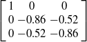$\left[\begin{array}{ccc} 1 & 0 & 0 \\ 0 & -0.86 & -0.52\\ 0 & -0.52 & -0.86 \end{array}\right]$ , T represents the translation matrix, with values of $[ 85.00 \,\, -582.68 \,\, -406.27 ]^{\text{T}}$ , and O represents the zero matrix. X _R , Y _R , and Z _R represent the three-dimensional coordinate values of the target in the robot coordinate system, respectively. 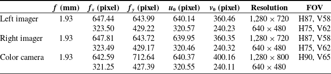In the second equation, $\left[\begin{array}{cccc} f_{x} & 0 & u_{0} & 0\\ 0 & f_{y} & v_{0} & 0\\ 0 & 0 & 1 & 0 \end{array}\right]$ represents the intrinsic parameter matrix, and f _x and f _y represent the equivalent focal length in the x-axis and y-axis directions, in pixels. After camera calibration, the intrinsic parameters of each imaging module of the Intel RealSense D455 were measured, and the key parameters obtained from the official technical documents [Reference Corporation27] are shown in Table VII. In addition, the baseline distance between the left and right imaging modules is 95 mm, and the field of view (FOV) of the infrared projector is H90° V63°.

Table VII.

Intel RealSense D455 intrinsic and key parameters.

Through the robot kinematic model and camera model, the three-dimensional coordinate information of the EE and the target workpiece can be obtained. Based on this, this paper designs a simple and efficient visual servo control strategy to achieve precise positioning and smooth movement of the Delta robot in a dynamic environment.

Let the current position of the EE be 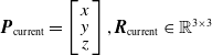$\boldsymbol{{P}}_{\text{current}}=\left[\begin{array}{c} x \\[-3pt] y\\[-3pt] z \end{array}\right], \boldsymbol{{R}}_{\text{current}}\in \mathbb{R}^{3\times 3}$ , and the target position be 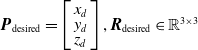$\boldsymbol{{P}}_{\text{desired}}=\left[\begin{array}{c} x_d \\[-3pt] y_d\\[-3pt] z_d \end{array}\right], \boldsymbol{{R}}_{\text{desired}}\in \mathbb{R}^{3\times 3}$ . Define the position error as $\boldsymbol{{e}}_{p}=\boldsymbol{{P}}_{\text{desired}}-\boldsymbol{{P}}_{\text{current}}$ . To ensure that the system has a quick response and good robustness in a dynamic environment, this paper employs a proportional-derivative (PD) control law. Let the control input be the desired velocity of the EE $\dot{\boldsymbol{{r}}}_{d}$ ; then the control law is designed as follows in Eq. (25):

(25) \begin{equation}\dot{\boldsymbol{{r}}}_{d}=\boldsymbol{{K}}_{p}\boldsymbol{{e}}_{p}+\boldsymbol{{K}}_{d}\dot{\boldsymbol{{e}}}_{p}\end{equation}

where K _p and K _d are positive definite gain matrices. This control law not only ensures the rapid attenuation of the error but also takes into account the dynamic response and anti-disturbance performance of the system. In order to obtain the joint control command, the relationship between the desired velocity $\dot{\boldsymbol{{r}}}_{d}$ of the EE in the operation space and the desired velocity $\dot{\boldsymbol{\theta}}_{d}$ of the joint space is also similar to Eq. (23), that is shown in Eq. (26):

(26) \begin{equation}\dot{\boldsymbol{\theta }}=\boldsymbol{{J}}\!\left(\boldsymbol{\theta }\right)\left(\boldsymbol{{K}}_{p}\boldsymbol{{e}}_{p}+\boldsymbol{{K}}_{d}\dot{\boldsymbol{{e}}}_{p}\right)\end{equation}

In order to verify the effectiveness of the control law, this paper uses the Lyapunov function method to perform stability analysis. Assume that the candidate Lyapunov function is shown in Eq. (27):

(27) \begin{equation}V=\frac{1}{2}\boldsymbol{{e}}_{p}^{\textrm{T}}\boldsymbol{{e}}_{p}\end{equation}

By selecting an appropriate PD gain, it can be satisfied that $\dot{{V}}\lt0$ , thus ensuring the global asymptotic stability of the closed-loop system.

5. Experiment

The system is deployed on a Delta robot platform equipped with an Intel RealSense D455 depth camera and Advantech EPC-P3086 industrial computer. The robot control frequency is set to 40 Hz to meet the requirements of high-speed operation. As shown in Figure 14, the model can achieve accurate segmentation on plastic workpieces, metal workpieces, glass workpieces, and EE.

Figure 14.

Instance segmentation.

As shown in Figure 15(a), the 3D trajectory of the EE while performing the grasping task. Figure 15(b) illustrates that the EE velocity smoothly converges to the desired value within 0.25 s, demonstrating the quick response and stability of the system, while also meeting practical production demands of 60−80 times per minute. The end-to-end latency, which includes perception at 17.2 ms, depth estimation at 3.4 ms, and control computation at 1.2 ms, totals 21.8 ms, satisfying the real-time requirement of 40 Hz.

Figure 15.

EE grasping, (a) trajectory, (b) velocity.

Record the endpoint pose of an experiment as $\hat{\boldsymbol{{T}}}=(\,\hat{\boldsymbol{{p}}}, \hat{\boldsymbol{{R}}})$ , with the ground truth target pose ${\boldsymbol{{T}}}^{*}=({\boldsymbol{{p}}}^{*}, {\boldsymbol{{R}}}^{*})$ . Where $\hat{\boldsymbol{{p}}}$ , p ^*, $\hat{\boldsymbol{{R}}}$ , and R ^* represent the actual and target position vectors and rotation matrices, respectively. The position error and the orientation error are defined as Eqs. (28) and (29):

(28) \begin{align} &\qquad\qquad\boldsymbol{{e}}_{p} =\left\| \hat{\boldsymbol{{p}}}-\boldsymbol{{p}}^{\textrm{*}}\right\|\\[-8pt]\nonumber \end{align}

(29) \begin{align} &\boldsymbol{{e}}_{\theta } =\arccos \left(\frac{\text{trace}\left(\boldsymbol{{R}}^{\textrm{*T}}\hat{\boldsymbol{{R}}}\right)-1}{2}\right) \end{align}

Let the task completion time be t _done . The time from the start until the first moment the condition is met and remains stable for more than t _hold seconds must be less than T _max. A single experiment is judged as Eq. (30):

(30) \begin{equation}\text{success}=\begin{cases} 1&\text{if }\boldsymbol{{e}}_{p}\leqslant d_{th}\wedge \boldsymbol{{e}}_{\theta }\leqslant \theta _{th}\wedge t_{done}\leqslant T_{\max }\\ 0&\text{otherwise} \end{cases}\end{equation}

Table VIII.

Comparison of visual servoing grasping methods.

Figure 16.

Convergence curves of grasping error, (a) X error, (b) Y error, (c) Z error, (d) θ error.

The task success rate (TSR) is calculated by Eq. (31):

(31) \begin{equation}{\textrm{TSR}}=\frac{1}{N}\sum _{i=1}^{N}\text{succes}{\textrm{s}}_{i}\times 100\mathrm{\% }\end{equation}

where the position threshold d _th = 0.01 m, the angle threshold θ _th = 5°, the time limit T _max = 5 s, and the stable holding time t _hold = 1 s.

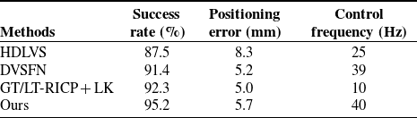
Furthermore, our method is directly compared with other existing visual servoing grasping approaches, as detailed in Table VIII. It can be seen that although the hybrid deep learning visual servoing (HDLVS) method proposed by Botezatu et al. [Reference Botezatu, Iancu and Burlacu28] can meet real-time requirements, its success rate and positioning accuracy need to be improved. The deep visual servoing feature network (DVSFN) method proposed by Luo et al. [Reference Luo, Zhang, Wang and Feng29] performs similarly to our method in terms of real-time capability and positioning accuracy, but still has a lower success rate. The GT/LT-RICP + LK method designed by Ruan et al. [Reference Luo, Ruan, Li and Chen30] combines the global template/local template-based RANSAC and iterative closest point unified algorithm (GT/LT-RICP) with Lucas-Kanade optical flow estimation. Although it has a high success rate and positioning accuracy, its control frequency makes it difficult to meet real-time requirements.

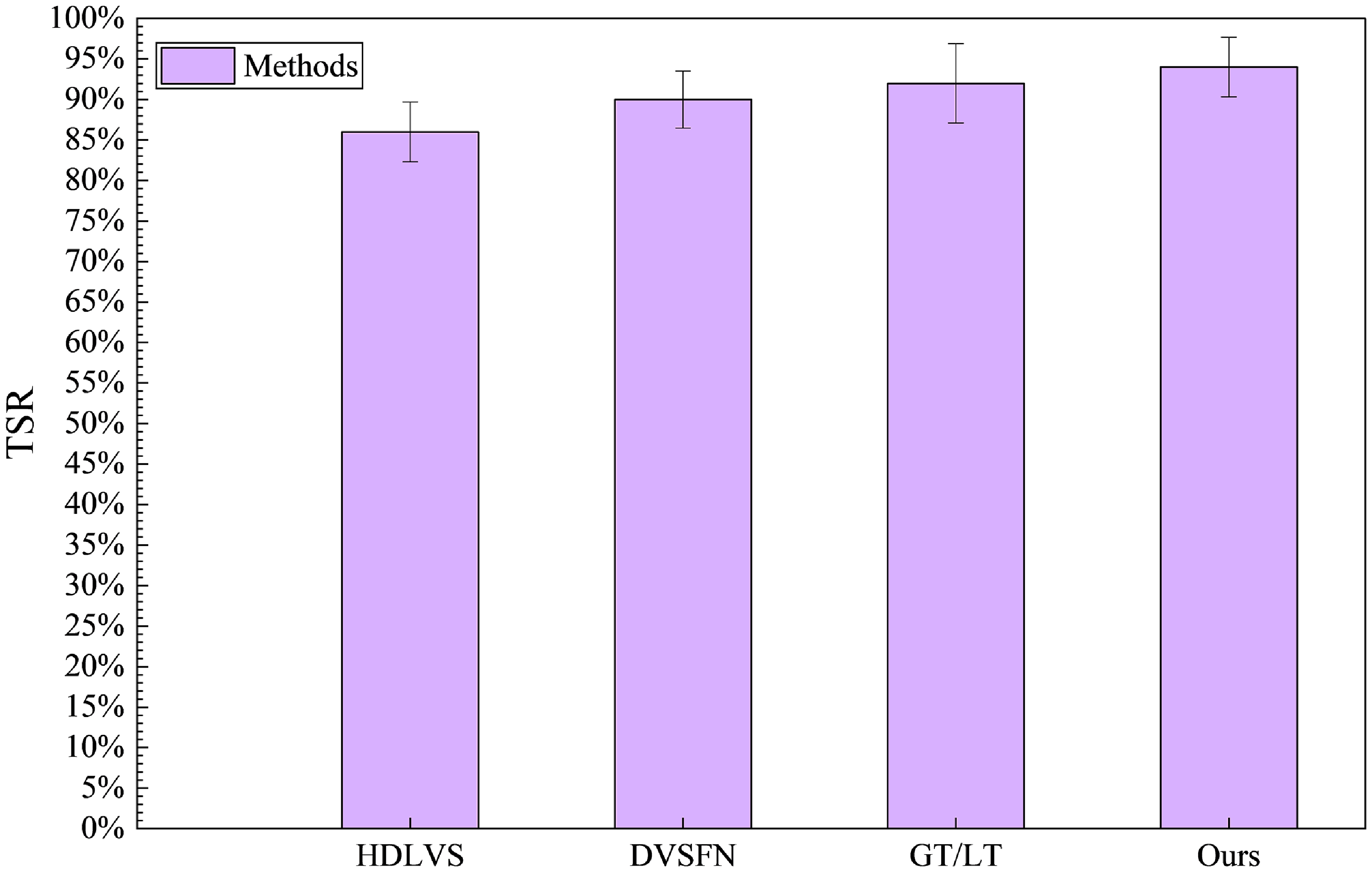
The displacement error curves, velocity error curves, and 3D trajectory comparison diagrams obtained from testing the above four methods are shown in Figures 16, 17, and 18, respectively. Conduct 50 parallel trials for each of the four methods, respectively, and obtain the TSR as shown in Figure 19. As shown in Figure 20, the image sequence of the robot grasping plastic, metal, and glass workpieces, respectively.

Figure 17.

Convergence curves of velocity error, (a) v_x error, (b) v_y error, (c) v_z error, (d) $\omega$ error.

Figure 18.

Trajectory comparison.

Figure 19.

Four types of vision servo TSR.

Figure 20.

Grasping image sequences.