INTRODUCTION
In recent decades efforts to reconstruct fire histories on decadal to millennial timescales have come to rely heavily on quantitative analysis of time series data developed from sub-fossil charcoal extracted from lake and wetland sediments. Algorithms that identify statistically significant positive anomalies (i.e., “peaks”) in the context of changing background values are commonly employed. Peaks are interpreted to represent fire events, which are then used to derive fire frequency, or the inverse, fire return intervals. The most widely used algorithm is the CharAnalysis software package (hereafter CharAnalysis; Higuera et al., Reference Higuera2009; Supplementary Section 1). Since its introduction in 2009, CharAnalysis has become the community standard for analysis and interpretation of charcoal timeseries as a proxy for fire event history (e.g., Mooney and Tinner, Reference Mooney and Tinner2011; Feurdean et al., Reference Feurdean, Spessa, Magyari, Willis, Veres and Hickler2012, Reference Feurdean, Liakka, Vanniere, Marinova, Hutchinson, Mosburgger and Hickler2013; Gill et al., Reference Gill, Williams, Jackson, Donnelly and Schellinger2012; Hawthorne and Mitchell, Reference Hawthorne and Mitchell2016; Iglesias et al., Reference Iglesias, Markgraf and Whitlock2016; Barhoumi et al., Reference Barhoumi, Peyron, Joannin, Subetto, Kryshen, Drobyshev and Girardin2019; Mariani et al., Reference Mariani, Tibby, Barr, Moss, Marshall and McGregor2019). This program has been critically evaluated with respect to statistical issues relevant to time series data (Higuera et al., Reference Higuera, Sprugel and Brubaker2005, Reference Higuera, Brubaker, Anderson, Hu and Brown2009, Reference Higuera, Gavin, Bartlein and Hallett2010a). Several excellent supporting studies on charcoal dispersal, transport, and depositional processes have informed and improved the methodological criteria (e.g., Clark, Reference Clark1988; Clark and Royall, Reference Clark and Royall1995; Lynch et al., Reference Lynch, Clark and Stocks2004; Tinner et al., Reference Tinner, Hofstetter, Zeugin and Conedera2006; Higuera et al., Reference Higuera, Peters, Brubaker and Gavin2007, Reference Higuera, Whitlock and Gage2010b).
However, studies aimed at assessing and improving CharAnalysis have focused primarily on landscape-scale processes and variables. A fundamental assumption remains untested: that charcoal deposition is a function of a homogeneous Poisson process. Specifically, this assumption states (Higuera et al., Reference Higuera, Gavin, Bartlein and Hallett2010a, p. 1003) “If charcoal count and volume data are available, then it is possible to assess the minimum increase in charcoal count required to be statistically greater than a previous sample, assuming measured counts are Poisson-distributed around the ‘true’ (unknown) count for a given sample volume.” This assumption pertains to the distribution of charcoal particles on a discrete horizon in the sediment column and accepts an individual sample from that horizon as representative of adjacent charcoal concentration at that level (i.e., “intra-level”). However, several critical aspects of charcoal deposition, including the pattern of particle distribution, the degree of homogeneity of the spatial distribution, the scales at which these distribution patterns hold, as well as the associated implications for sampling uncertainty (and hence reproducibility) have not yet been assessed.
In order for the probability thresholds in CharAnalysis to be appropriate, intra-level count variability, or sampling uncertainty, must be lower than the thresholds defining the probability of inter-level populations being statistically similar or different, and those used to distinguish between noise and signal in the time series. In other words, defining sampling uncertainty requires understanding how counts may vary across the plane of sampling, at the scale of the sample. For objective identification of significant count differences between levels in a sediment core, the thresholds must be scaled to the population variance and resultant sampling uncertainty from within an individual level. However, the probabilities calculated in CharAnalysis are based on the variability observed in the temporal domain, but not in the spatial domain. This absence of consideration of the spatial domain has important implications for how well CharAnalysis parses signal from noise, and how well the Minimum Count Test (MCT) works as a final assessment of peak significance. To our knowledge, this is the first study to assess intra-level charcoal count variability and its effect on quantitative peak detection.
The original impetus for the current study arose from observations made by Schlachter and Horn (Reference Schlachter and Horn2010, p. 701) in which they stated that “Horizontally adjacent samples from the same core may vary in charcoal concentration.” Schlachter and Horn (Reference Schlachter and Horn2010, p. 707) further noted that “Differences between charcoal concentrations measured in the same stratigraphic depths suggest that inferences about changing fire history based on small shifts in charcoal curves may not be justified.” The need for an explicit examination of intra-level charcoal count variability was further clarified in an exploratory study conducted in our laboratory in which initial results showed significant count differences between samples drawn from within the same level of a single core. This prompted development of the current study in order to systematically evaluate count variance of intra-level charcoal samples.
Previous studies have used replicate count data to assess the reproducibility of macroscopic charcoal analysis. For example, Whitlock and Millspaugh (Reference Whitlock and Millspaugh1996) conducted an elegant replicate study in which they examined variability of charcoal counts from core transects taken across multiple lake basins, as well as in multiple cores recovered from a single location. The upper 2 cm of sediment from replicated cores were analyzed for intra-site comparison. Results showed coefficients of variation that were quite large, ranging from 17.6% for a mean concentration of 29.2 particles/cc, to 49.4% for a mean concentration of 8.5 particles/cc. However, the methodology called for the 2 cm thick by 5 cm diameter core sections to be homogenized before subsampling by aliquot. Consequently, these findings do not address the question of intra-level variability referenced in the Schlachter and Horn (Reference Schlachter and Horn2010) study.
More recently, Walsh et al. (Reference Walsh, Anderson, Deardorff, Johnson, Kim, Mitre and Morrey2021) published a study in which multiple cores were recovered from two lakes and the charcoal influx records of each core were compared for qualitatively similar patterns. Their findings showed the general shape of charcoal curves in adjacent cores to be similar. Their study again differs from ours in that the counts are from adjacent cores, and the study does not analyze the charcoal records quantitatively.
Here we present an analysis of replicated samples from sediment cores taken in three different lakes, each with a distinct geographic setting and depositional environment. This is not an attempt to reconstruct fire history, nor is it an attempt to validate or calibrate peak detection methodology with known fire events or regimes. This is a numerical exercise intended to assess replication of peak detection results using replicated intra-level count data from within individual cores. Our null hypothesis (Ho) is: iterated CharAnalysis runs using replicate intra-level charcoal count data will replicate peaks at a rate of at least 95%.
This study addresses three questions that arise from assumptions relied upon by CharAnalysis. (1) Within a discrete level of a sediment core, are charcoal particles Poisson distributed in space? (2) What is the rate of peak reproducibility when replicate data are run iteratively through CharAnalysis? (3) Is the MCT, as applied by CharAnalysis, appropriate as a last test for significance in distinguishing the probability of whether charcoal particle counts come from similar or distinct populations?
In order to address these questions, we used replicated charcoal particle count data from three lake sediment cores to (1) test for Poisson distributions in the sampled populations, (2) test the rate of reproducibility for peaks detected using CharAnalyis, and (3) examine the appropriateness of the thresholds used to determine significance of detected peaks. We detail our methods below and have included the code and all data in order that other researchers may replicate this study with our, or their own, data.
METHODS
Core recovery and site descriptions
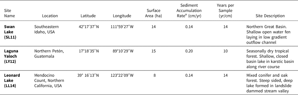
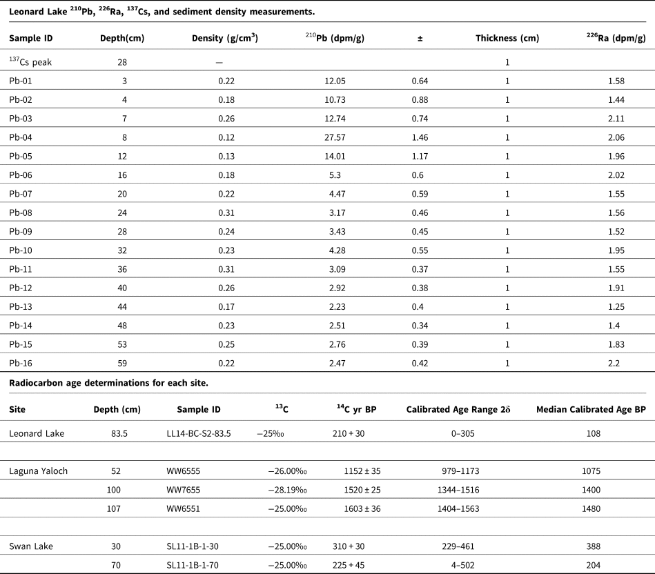
Replicate sample datasets were developed from three sites, each with different depositional conditions and sediment characteristics. A summary of site characteristics, including sedimentation rates and sampling resolution for this study, is shown in Table 1. Age control for sampled sections is shown in Table 2.
Site names, locations, and site descriptions for cores used for replicate charcoal particle counts.

a Accumulation rates and yr/cm are for sections of core sampled in this study.
Age control measurements by site.

Leonard Lake (39° 16′13″N, 123°22′09″W) is a small lake located in the Northern Coast Ranges of Mendocino County, California, U.S.A. It formed ca. 4000 years ago when a deeply incised stream was dammed by landslide activity, resulting in an ~81 ha catchment. The lake occupies a narrow, steep sided valley. The surface of the lake is ~8 ha, with a water depth of ~16 m at the coring site. At the southern end of the lake is low gradient marsh and meadow habitat formed by infilling via the primary stream. The majority of the shoreline and watershed is characterized by steep slopes supporting mixed douglas fir and redwood forest. The sediment from Leonard Lake used in this study is comprised of finely laminated gyttja. Sampled depths were from 18–78 cm. Age control is from 16 210Pb measurements, 237Cs peak depth, and one radiocarbon age determination.
Laguna Yaloch (17°18′35″N, 89°10′29″W) is a shallow, closed-basin lake formed in a karstic basin along the middle course of the Holmul River, eastern Petén, Guatemala. The surface of the lake is ~15 ha, and water depth at time of coring was 1.15 m. Surrounding vegetation ranges from dense closed-canopy forest in the upland areas to shrubs and grasses in the lowest areas (Lundell, Reference Lundell1937; Fedick and Ford, Reference Fedick and Ford1990). The section of the Laguna Yaloch core used in this study is from 50–110 cm. The sediment is comprised of fine-grained peat. Age control for this section is based on four radiocarbon age determinations.
Swan Lake (42°17′37″N, 111°59′27″W) is a shallow carbonate fen currently containing a shallow pond. The site is located in southeastern Idaho, U.S.A., at the northeastern extent of the Great Basin. It lies in the overflow channel of pluvial Lake Bonneville. At the time of coring, open water extent was ~14 ha, and water depth was ~35 cm. The section of sediment core from Swan Lake used in this study is comprised of laminated carbonate mud, and extended from 0–60 cm. Age control was based on two radiocarbon age determinations.
All cores were recovered using 7 cm diameter polycarbonate tubes fitted to a Bolivia piston corer and deployed from a floating platform. Cores were stored in the core repository refrigerator at the United States Geological Survey (USGS) facility in Menlo Park, California, USA. Sediment cores were maintained at 3°C, except when being actively split, imaged, or sampled. All laboratory procedures, counting, and data analyses were carried out in the Quaternary Paleoenvironmental Research Laboratory (Q-PRL) at the USGS, Menlo Park.
Sampling, processing, and counting protocols
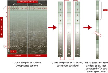
Cores were split and sampled at thirty (30) contiguous, 2 cm thick levels. Twenty (20) 1.25 cc samples were taken at each level. This sampling protocol was informed in part by a survey of the Global Charcoal Database (Marlon et al., Reference Marlon, Kelly, Daniau, Vannière, Power, Bartlein and Higuera2016a, Reference Marlon, Kelly, Daniau, Vannière, Power, Bartlein and Higuerab), wherein a 1cc sample size is the most commonly used sample volume for paleo fire studies based on particle counts (Supplementary Fig. 1). The split surfaces of the cores were cleaned to eliminate down-core contamination resulting from the splitting process. Ten consecutive 1.25cc samples (0.5 × 2 cm) were taken from each half to create a total of 20 samples (Fig. 1). Each sample was cut from the split core using a square tipped spatula and measured for volume in a measuring spoon. Care was taken to leave the layer of sediment closest to the liner to avoid contamination by dragging along the outside of the core, which can occur during the coring process. For each level, samples were taken in a crosswise progression in order to track the proximity of samples relative to each other.
Schematic of replicate sampling and artificial core “construction.”

Appropriate bleaching time was determined using preliminary experimental extractions (Anderson and Wahl, Reference Anderson and Wahl2016). Samples were processed in batches of 20 so that all samples from a single level were treated together. Each sample was placed in a 50 ml test tube in 10 ml of 3% sodium hexametaphosphate solution for 24 hours to initiate deflocculation. Clorox® bleach was used to remove non-charcoal organic matter and to complete deflocculation. Thirty (30) ml of bleach (6% sodium hypochlorite) was added, and test tubes were laid on test tube rollers for 1 hour. In order to achieve consistent bleaching times, samples were first decanted into 4” sieves sitting in a water bath deep enough to submerge the surface of the sieves. Samples then were sieved at 125 μm, and the >125 μm fraction was washed into disposable petri dishes. Petri dishes were dried in an oven at 50°C for 72 hours.
Counts were performed manually using a binocular scope at 5–15x magnification. A 0.5 × 0.5 mm gridded “coaster” was placed under the petri dishes to facilitate systematic movement of the dish to insure complete coverage. All charcoal particles were tallied, and counts were entered into spreadsheets. Counts were performed by a team of three technicians. In order to establish consistency, initial counts were replicated by all three technicians to verify that counts for the same petri dish by different technicians were within 10% of each other. Following this visual “calibration,” all intra-level counts were performed by a single technician. All sample counts that fell beyond two standard deviations from the mean for the level were re-counted by the lead author. If no replicates for a level exceeded the two standard deviation range, then the maximum and minimum counts for that level were re-counted. For the Laguna Yaloch samples, due to very high counts and wide-ranging values, 5–9 samples for each level were re-counted by the lead author. One sample from Laguna Yaloch (level 8, replicate 20) was rejected due to insufficient clearing of the sample in preparation. An abundance of dark debris effectively precluded reliable identification of charcoal. In this instance a value equal to the mean of the other 19 samples from level 8 was assigned for the count value of replicate sample 20.
Data Analysis
All analyses, including data treatments for CharAnalysis input, were performed using the opensource R statistical software (R Core Team, 2018). All code developed for execution of the methods described below is available for use at the USGS Gitlab link (https://code.usgs.gov/gmeg/replicatechar).
Artificial cores and synthetic data
Artificial cores were created in order to form time series of sufficient length to be evaluated in CharAnalysis (Figure 1). Terminology used in the discussion of the artificial core creation is defined here:
Level = A single, 2 cm thick horizontal plane from which 20 replicate, intra-level samples were taken. There are 30 contiguous levels per core.
Replicate = Charcoal counts from within a single level (intra-level counts). There are 20 replicates per level.
Original count = Charcoal particle counts from actual subsamples.
Synthetic count = Poisson distributed count values generated based on the means of each level's 20 replicate original counts.
Set = Consecutive count values (either original or synthetic) from 30 contiguous levels. When creating a set, levels remain true to the stratigraphic position from which they were taken from the core (i.e., while replicates from a level may be randomly chosen, levels 1–30 always remain in fixed order in every set).
Artificial core = Twenty (20) contiguous sets strung together end on end, resulting in an artificial “core” comprised of 600 values. This artificial core utilizes the data in a way that can be processed by CharAnalysis.
Artificial cores were constructed for each site to test the expected outcome (Ho) of a fire frequency curve that is either flat or has a consistent periodicity that repeats in synchroneity with the repeating sets throughout the core. Four types of data were analyzed:
Sum of All: All 20 replicate counts for each level are summed. The result is a set that has count values for each level equal to the sum of all intra-level counts. Because the same data are used in each set, this dataset establishes what results would look like if intra-level count variability was insignificant, and what we would expect to see if our null hypothesis is correct. (1) A synthetic core is constructed with the same set of summed levels repeated 20 times. (2) Three artificial cores based on Sum of All data were generated, one for each site.
Original Data, Random (with replacement): One count value was randomly selected from each level in a set. Sets were compiled into artificial cores and analyzed to test reproducibility given the actual within-level variability. (1) Sets are created by randomly selecting one replicate from each level (with replacement). (2) Twenty sets are stacked to produce an artificial core. (3) One thousand artificial cores were generated for each site.
Synthetic Homogeneous Aliquots: Synthetic data were created around the mean value for each level. This analysis tests the effect of a Poisson distributed sample distribution on reproducibility of results. (1) Based on the mean of the 20 replicate original counts for each level, a set of Poisson distributed counts were generated. Values were then randomly selected, from the generated data for each level to create 20 synthetic sets. (2) These 20 synthetic sets are stacked to create an artificial core. (3) One thousand artificial cores were generated for each site.
Synthetic Heterogeneous Aliquots: Similar to Homogeneous Aliquots, but using resampled count data to calculate a different mean for each Poisson distribution generated. This analysis introduces an additional degree of freedom in testing reproducibility. Poisson distributed counts were constructed based on multiple means derived from bootstrapping of original count data by level. (1) For each level, a mean of a bootstrapped sample population (n = 20) is calculated. (2) A set of 20 Poisson distributed values is generated around that mean. (3) A random value is selected from the generated Poisson distribution. (4) Repeat steps 1–3 30 times, once for each level, to create a set. (5) Repeat step 4 20 times to create 20 sets for one artificial core. (6) One thousand artificial cores were generated for each site.
Test for over dispersion
CharAnalysis assumes that counts are drawn from distributions with means fixed at each sampled horizon such that intra-level counts will be Poisson distributed in space around this mean (Higuera et al., Reference Higuera, Gavin, Bartlein and Hallett2010a). Using replicate intra-level samples (20 per level) we are able to test this assumption. Given that a condition of a Poisson distribution is the ratio of σ : μ = unity, the null hypothesis for this test is Ho: σ = μ. The alternative to this hypothesis is over-dispersion among the replicated counts. That is, there is higher variance relative to the mean than would be expected in a Poisson distribution.
To determine the probability of overdispersion in the original count data, we generated sets of means and standard deviations for each level using a bootstrap approach on the counts. Under the null hypothesis, a Poisson distribution for the population of counts will have a sample count sum equal to the true population mean, scaled by the number of samples. Conditional on (that is, fixing) this sum, the individual counts are multinomially distributed, all with equal probability. Using original count sums for the levels, we generated a large number (n = 1000) of multinomially distributed sets of random values and calculated the standard deviation for each set. This provided us with an estimate of the distribution of standard deviations. We then compared these standard deviations to the standard deviation of the intra-level original counts. The quantile into which the original replicate's standard deviation falls in the distribution of the generated standard deviations provides us with a probability for acceptance or rejection of the null hypothesis.
Minimum count test (MCT)
Maximum intra-level count differences for each level were compared to the threshold curves derived from the minimum count test (MCT) used in CharAnalysis. This test is used as a final check to screen potential peaks for values that, although they exceed the locally defined thresholds, may still be statistically insignificant (Detre and White, Reference Detre and White1970; Shiue and Bain, Reference Shiue and Bain1982; Higuera et al., Reference Higuera, Gavin, Bartlein and Hallett2010a; see section 2.3.5 below). Here we apply this test to determine the probability that two counts from within the same level come from different Poisson distributions (Higuera et al., Reference Higuera, Gavin, Bartlein and Hallett2010a). The MCT examines count values and compares the minimum count (X1) and sample volume (V1) and the maximum count (X2) and sample volume (V2) according to the following equation:

Critical values used for infinite degrees of freedom (two tailed t-test) are: alpha = 0.05; Z = 1.9600 and alpha = 0.01; Z = 2.5758. A Poisson distribution is assumed, and the d statistic is compared to the Student's t distribution. The probabilities of maximum and minimum counts coming from different Poisson populations were tested at 95% and 99% confidence levels. The differences for counts (x1 − x2) and percentages ([x1 − x2]/x1 ×100) were compared to the critical value threshold.
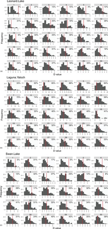
The maximum difference value represents a “worst-case-scenario” for each level. To examine a more nuanced view of the range of intra-level count variation, and the probability of intra-level differences being considered statistically significant by the MCT, the d-statistics for all 190 possible pairwise differences between the 20 replicated sample values for each level were calculated. The resulting probability distributions were plotted along with the MCT threshold at 95% probability.
CharAnalysis
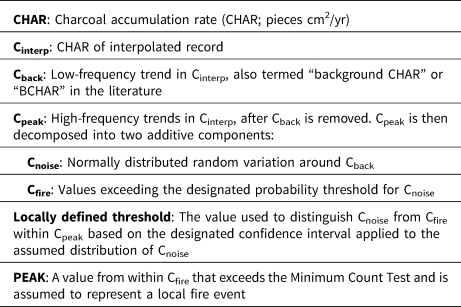
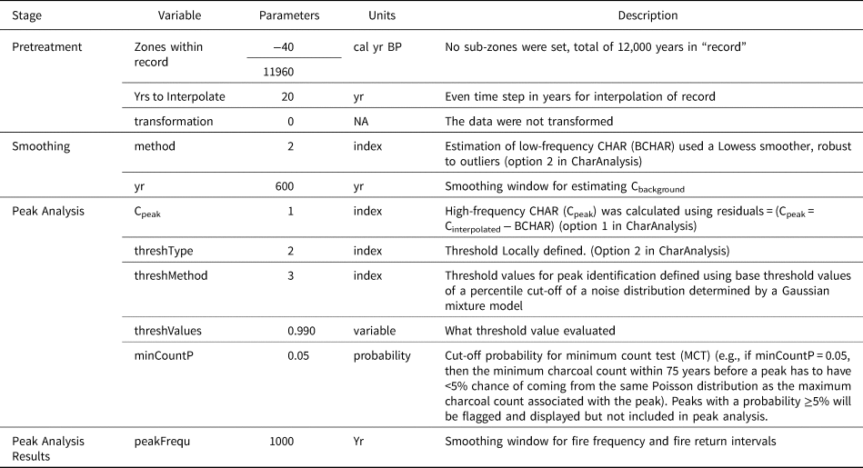
The artificial cores were analyzed with the CharAnalysis program (Higuera et al., Reference Higuera, Brubaker, Anderson, Hu and Brown2009, Reference Higuera, Gavin, Bartlein and Hallett2010a; Kelly et al., Reference Kelly, Higuera, Barrett and Hu2011; freeware available at http://phiguera.github.io/CharAnalysis/). Terms used in this discussion are defined in Table 3 (Higuera, Reference Higuera2009). In essence, the algorithm decomposes the interpolated charcoal influx variability into background (Cback) and non-background (Cpeak). Cback is assumed to represent low frequency changes in charcoal influx, not related to local fires; Cpeak is assumed to include the local fire signal but must undergo further analysis to identify local fire events. To accomplish this, Cpeak values are evaluated for consideration as potential fire events (Cfire) against a locally defined threshold to remove the random noise component (Cnoise, see below). To validate the statistical significance of the potential fire events, Cfire values are then subjected to a MCT. Cfire values that pass the MCT are designated as peaks, which indicate local fire events. Because the nomenclature around CharAnalysis output varies somewhat in the literature, in the remainder of this discussion we will refer to values that pass both the noise threshold test and the MCT as PEAKs, which is the peak component that CharAnalysis identifies as characterizing local fire events. As a final step, CharAnalysis calculates a signal to noise index (SNI) as a metric to evaluate the strength of the distinction between the signal and noise components of the time series (see below).
Definition of terms used in the description of CharAnalysis.

Following is a detailed description of how the CharAnalysis algorithm moves through each step. Input data are time series of charcoal counts, sample volumes, depths, and modeled ages at each depth. Charcoal accumulation rate (CHAR) is then calculated by dividing charcoal counts in each sample by the time interval represented in that sample.
Cinterp is then calculated by converting original counts to concentration (particles/cc) and interpolated into even time steps based on a user designated time parameter; in this study, counts were interpolated to timesteps of 20 years per 2 cm depth increment.
Cback, which is the background component of the CHAR data, is then calculated. Cback is assumed to be comprised of low frequency CHAR variations driven by environmental factors other than local fire, such as redeposition, bioturbation, and distant fires (Higuera et al., Reference Higuera, Peters, Brubaker and Gavin2007). It is defined using a smoothing algorithm within a moving window. Several methods are available (moving mean, moving median, moving mode, Lowess smoother, or Lowess smoother/robust to outliers). Our analyses used the Lowess smoother/robust to outliers method.
Cpeak is derived. This component is the series of detrended CHAR values is created by removal of Cback. It can be calculated as either a residual of Cback (CHAR − Cback) or as a ratio (CHAR:Cback). In this study, we use the residual method.
Cpeak is then further analyzed to parse out two components: Cpeak = Cnoise + Cfire, in which Cnoise = normally distributed variation around Cback, and Cfire = values exceeding Cnoise.
Distinguishing the fire signal (Cfire) is next. As mentioned above, Cpeak is composed of two additive components: Cnoise + Cfire = Cpeak. A Gaussian mixture model (Bouman et al., Reference Bouman, Shapiro, Cook, Atkins, Cheng, Dy and Borman2005; Gavin et al., Reference Gavin, Hu, Lertzman and Corbett2006; Higuera et al., Reference Higuera, Brubaker, Anderson, Brown, Kennedy and Hu2008, Reference Higuera, Gavin, Bartlein and Hallett2010a) is used to establish a local threshold in order to distinguish the Cnoise component of the positive Cpeak population. The Cpeak values that clear the threshold are then considered Cfire. The distribution of Cfire does not need to be known because Cnoise is assumed to have a normal distribution. As such, values of Cpeak that fall into the extreme positive tail of the probability distribution of Cnoise (i.e., Cpeak values above the locally defined threshold) are designated as Cfire. Taking the Cback value at the center of the window as zero, the Gaussian mixture model is applied to the Cpeak values within the smoothing window. For a 600 year window, the Cpeak values within 300 years before and 300 years following the center increment would be considered. The Gaussian mixture model distinguishes the two component populations within the Cpeak values: Cnoise and Cfire. Each of these two component populations has a different mean and variance, and distinct proportional contributions to the total Cpeak population. The Cnoise population is defined as the distribution having the lower mean (smaller values), corresponding to relatively small departures from Cback. The Cfire population encompasses the variability that diverges widely from the background (ideally these two populations are quite distinct from each other). By referencing the assumed Cnoise distribution, a threshold is derived such that Cpeak values exceeding a designated confidence interval (here the 95th percentile) comprise the Cfire component of Cpeak. The threshold value is calculated sequentially for each consecutive window in the time series. The Cfire component contains all possible PEAK values (note that Cfire is labeled ‘peak’ in the CharAnalysis output).
Minimum count test (MCT) and PEAK determination are next. The PEAK component (not to be confused with Cpeak) represents the “signal of interest” (Higuera et al., Reference Higuera, Gavin, Bartlein and Hallett2010a), indicating discrete local fire events. As a final test to distinguish local fire events, Cfire values are subjected to the minimum count test referenced above. This is done to exclude Cfire values that exceed the locally defined noise threshold value, yet may be statistically insignificant. The MCT (first introduced in “CHARSTER” by Gavin, Reference Gavin2008) applies equation 1 to the original raw count values (not interpolated) to compare the minimum count (X1) and sample volume (V1) falling within the preceding 75 years of the potential PEAK, and the maximum count (X2) and sample volume (V2) falling within the 75 years following the potential peak (Higuera, Reference Higuera2009). A Poisson distribution is assumed, and the d statistic is compared to the Student's t distribution. If there is a >5% chance that the maximum and minimum counts have come from the same Poisson distribution, the potential PEAK is rejected. Values that pass the MCT are designated as PEAKs and assumed to represent local fire events (‘peaks Final’ in the CharAnalysis output) (Shiue and Bain, Reference Shiue and Bain1982; Higuera, Reference Higuera2009; Higuera et al., Reference Higuera, Gavin, Bartlein and Hallett2010a). Again, for clarity, in this discussion we refer to the Cfire values that pass the MCT as PEAKs. PEAKs then are smoothed with a moving window to present changes in fire frequency through time. In this study a 1000-year smoothing window was used.
We designated an age model and CharAnalysis parameters similar to those used for example data provided with CharAnalysis, and to those used in previously published methodological evaluations of CharAnalysis (Higuera et al., Reference Higuera, Gavin, Bartlein and Hallett2010a; Kelly et al., Reference Kelly, Higuera, Barrett and Hu2011). A deposition time of 20 years per 2 cm interval was assigned, giving each artificial core an “age” of −40 to 11,960 years BP. It is worth noting that the time and depth intervals used here are not of particular significance. As long as the values are constant between runs, the comparison of the replicated counts remains valid. The depth interval could be changed to 1 cm, for example, and it will not affect the results. Alternatively, if the interpolation interval were changed to 40 years, and the window widths and age estimates were also doubled, the results would likewise remain unaffected. Cback was calculated using a Lowess smoothing, robust to outliers, within a 600 year window, which ensured the recommended minimum of 30 values in each window (Higuera et al., Reference Higuera, Brubaker, Anderson, Hu and Brown2009) and falls within the window width typical for most studies using CharAnalysis (Higuera et al., Reference Higuera, Gavin, Bartlein and Hallett2010a). Parameters were held constant for all runs and are presented in Table 4.
Parameters used in all CharAnalysis runs.

Signal to noise index (SNI)
CharAnalysis uses a signal to noise index (SNI) (Kelly et al., Reference Kelly, Higuera, Barrett and Hu2011) to determine which sections of the time series are reliably recording fire events. For each moving window, noise and signal are treated as distinct populations (N and S, respectively) separated by a threshold set near the upper limit of the noise distribution. The signal (S) contains the values in Cpeak (the residuals after Cback is removed) exceeding the threshold; the noise population (N) contains all Cpeak values equal to or less than the threshold for a specific time window:

Here ns is the number of values in S and nN is the number of values in N. The mean and standard deviation of the values in N are $\bar{N}$ and σ N, respectively, and S1, S2…Sn are the individual values in S. The equation scales the separation of signal and noise by the standard deviation of the noise population within the moving window. Thus, the SNI value provides an intuitive measure of how divergent the two populations are. For example, assuming a normal distribution in the noise population, SNI = 3 would indicate that the mean for the signal population falls at least 3 standard deviations above the mean of noise. Kelly et al. (Reference Kelly, Higuera, Barrett and Hu2011) recommended that sections of the record in which SNI < 3 be discussed in terms of changes in background values only. In order to evaluate the relationship between signal strength and PEAK reproducibility, PEAKs were binned by SNI values.
Similarity Index
To quantify the degree of similarity in PEAK identification between the runs, a Jaccard index (Chung et al., Reference Chung, Miasojedow, Startek and Gambin2019) was calculated for the runs based on the count data. Sets were compared pairwise from randomly selected runs such that:

Where J is the index of similarity between the sets X and Y, where is all of the peaks shared by each set and are all of the peaks that occur in either set. Two identical sets would have an index of 1, while completely dissimilar sets would have an index of 0.
RESULTS
Our findings reveal the following. (1) The test for overdispersion shows that only 9% of the replicate counts have a probability >5% of originating from a Poisson distribution. (2) The maximum rate of peak replication based on iterated intra-level counts is 60%. (3) The 95% probability threshold calculated for the noise distribution is spurious given the intra-level count variability. (4) Intra-level count differences were larger than the MCT threshold used to identify statistical significance in inter-level count differences in over 90% of the data.
Several unanticipated outcomes are also significant. (1) Even when a Poisson distribution is imposed using synthetic data, in only one instance did the peak detection rate exceed 95%. (2) Inconsistences in the results were not resolved by increasing the signal to noise index (SNI) threshold as a criterion for confidence in fire frequency reconstructions. (3) A pronounced “edge effect” is observed at the very top and bottom of the artificial cores, calling for caution when attempting to calibrate CharAnalysis output from the most recent sections of sediment cores with instrumental, historical, or tree ring (fire scar) data.
Original counts, analysis of over dispersion, and within-level count differences (MCT)
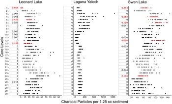
Our results provide strong evidence that charcoal distribution in all three cores does not conform to a Poisson distribution in space (Fig. 2). Only 9% of the 90 intra-level original count distributions have >5% probability of originating from a Poisson distributed population. In other words, data from >90% of the levels do not support the null hypothesis of sample counts being derived from a Poisson distribution. The descriptive statistics for original counts by level and by site are shown in Supplementary Table 1. Full data sets are included in Supplementary Table 2, as well as count data presented in the order and relative proximity of samples taken from the sediment (Supplementary Table 3a–c).
Dot plots of intra-level original counts from three sites and probabilities of the observed counts originating from a Poisson distribution. Levels in red indicate distributions with a >0.05 probability of being Poisson distributed. The y-axes represent levels sampled. Note the different ranges on the x-axes. All counts represent particles per 1.25 cc. See methods section for full discussion of sampling and counting protocol.

These data exemplify the range of particle concentrations typically found in lake cores, in that the three sites include low counts at Leonard Lake, moderate counts at Swan Lake, and both extremely high and moderate counts at Laguna Yaloch. Leonard Lake (LL14) minimum and maximum particle counts for the entire core range from 0–93, and the maximum intra-level difference for the core is 64 (min = 7, max = 71). The coefficient of variation (CV = standard deviation/mean), an intuitive measure of dispersion of values, ranges from 21.5–70.3%. Laguna Yaloch (LY12) has minimum and maximum counts of 15 and 1,679 particles, with a maximum intra-level difference for the core of 1,569 (min = 110, max = 1679), and the CV ranges from 12.2–91.0%. The Swan Lake (SL14) minimum and maximum are 17 and 146 particles, the maximum intra-level difference for the core is 108 (min = 24, max = 132), and the CV ranges from 9.6–45.2%.
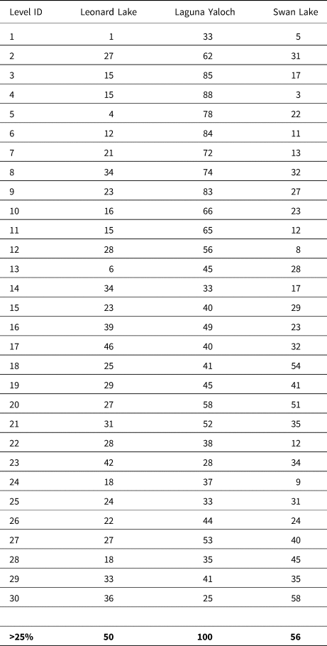
The count differences from within all levels counted include ranges large enough for counts from within the same level to be flagged as originating from different populations at both 95% and 99% probability (Supplementary Section 2; SI Fig. 2). The probability distributions of the d-statistic for all 190 possible count differences between the 20 intra-level values for each level compared against the MCT threshold are shown in Figure 3a–c and Table 5. For Laguna Yaloch, 25% of the differences fail the MCT in 100% of the levels. Data from Leonard Lake and Swan Lake show a failure rate of 25% or more for 50% and 56% of the levels, respectively.
(a–c) Histograms showing frequency (gray bars) for all 190 possible differences between the 20 replicated values at each level compared against the MCT threshold (vertical red line). Values in upper right of each plot indicate the proportion of difference values that are statistically significant for the level. (Figure continued on the following pages).

Percentages of all possible count differences with d-statistic larger than MCT threshold, per level, in each core. Bolded numbers indicate the percentage of levels for each site in which >25% of the possible differences exceed the MCT threshold. All values shown as percent.

PEAK detection and smoothed fire frequencies
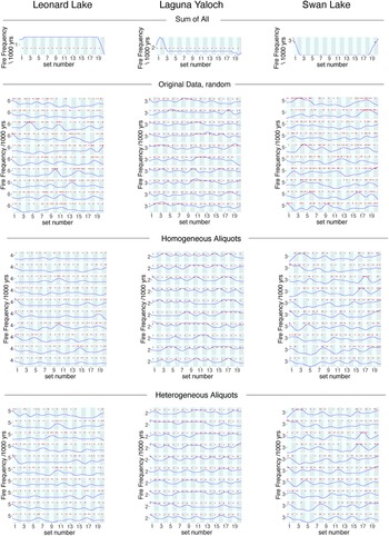
CharAnalysis results showing fire events (PEAKs) are presented in Figure 4. Fire frequency is plotted for qualitative comparison of the runs to illustrate the effect of different PEAK detection results on the frequency curves. A representative set of replicate CHAR values is shown in Supplementary Figure 3. The Sum of All analysis for each site shows PEAKs occurring at regular intervals along the cores, as expected, because these cores were constructed by repeating sets of the same 20 summed intra-level values for each level. As a result, PEAKs occur at the same levels in each set, creating a consistent periodicity in the fire frequency, except, importantly, where edge effects influence the results. For all three sites, edge effects appear to influence between 30–60 levels (one to two sets) at the beginning and end of the record. The Sum of All plots represent what would be expected in plots from the other three analyses conducted with these data if there was little or no variability in intra-level count values. A randomly selected group of 10 plots (of the 1000 cores generated) is shown for the three data treatment methods (Fig. 4). Variability in fire frequencies is highest for reconstructions based on the Original Count, Random data at all sites. Some improvement is shown in the range of smoothed frequencies corresponding to the Poisson distributed data analyzed in the Homogeneous Aliquots and Heterogeneous Aliquots for all sites, but notable inconsistencies persist.
Representative examples of replicated CharAnalysis runs, randomly selected, form 1000 iterations. Red + indicates peaks detected with 600 year moving window. Blue curve represents fire frequency smoothed with 1000 year moving window. Sum of All: single run using repeating values (note edge effects in Sum of All curves for all sites). Original Data, random: selection, with replacement, from original replicate count data. Homogeneous Aliquots: sampled from synthesized, Poisson distributed data based on means of original counts (this simulates mixing and then subsampling all the sediment sampled in each level). Heterogeneous Aliquots: sampled from synthesized, Poisson distributed data, based on means derived from resampling of original counts. Results are shown with the x-axis indicating sets to clearly indicate the bounds of repeating sets in the artificial cores.

PEAK detection replicability and SNI
For the purposes of this discussion, “opportunity” is defined as a chance for one of the intra-level original or synthetic count values from a given level to be identified as a PEAK. Because sets are appended to create the artificial cores, each level of each artificial core scenario has 20,000 opportunities (1000 simulations × 20 sets per artificial core) for a level to be associated with a PEAK. Here, we define significant-positives as PEAKs detected with SNI >3 in 95% or more of the opportunities within a level. Insignificant-positives are PEAKs detected with SNI >3 in >5%, but <95%, of the opportunities. The peak detection rate is the percentage of peaks identified as a proportion of the opportunities.
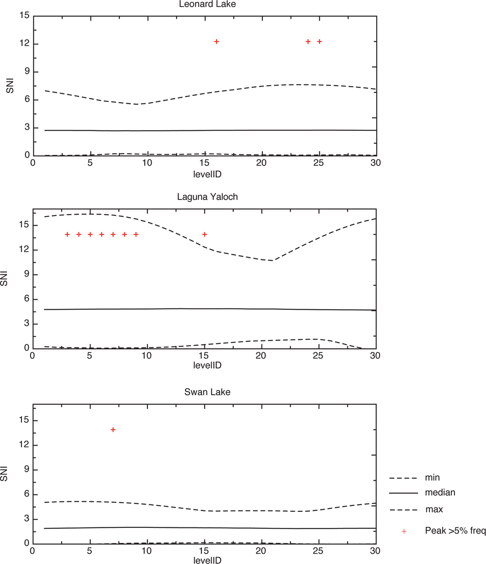
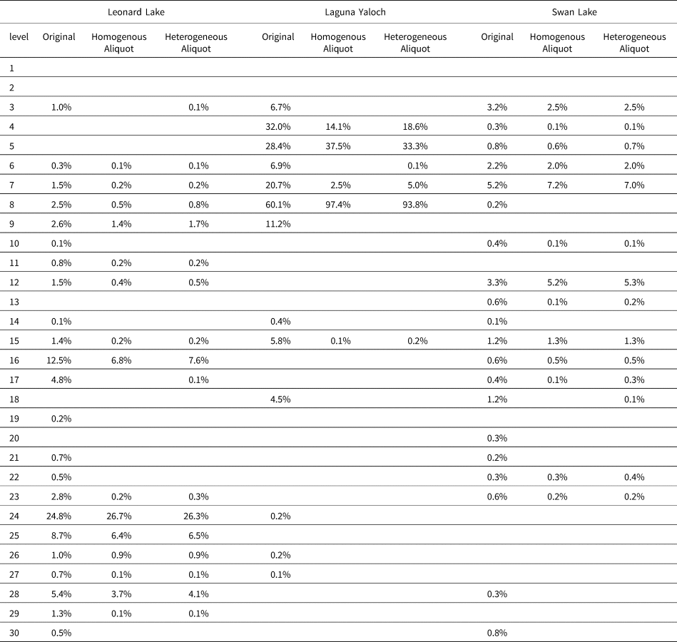
The range and median of the SNI are presented in Figure 5, by site and level. All three sites show a SNI ≥3 for the set. Table 6 presents the percentage of opportunities from each core that indicate PEAKs with a SNI >3 that were detected in the 1000 CharAnalysis runs (excluding sections affected by the edge effect; n = 16,000 opportunities, blank cells represent no PEAKs detected). For the intra-level count data, the highest rate of detection for a peak is 60.1% at level 8 in Laguna Yaloch. If levels 7 and 8 are combined, the detection rate increases to 80.8%, and if 7, 8, and 9 are combined, the detection rate sums to 92%. Only one significant-positive occurs (≥95% rate of a PEAK being detected at a level) corresponding to level 8 in the synthetic Homogeneous Aliquots data from Laguna Yaloch.
Signal to Noise Index (SNI) by level for 1000 random with replacement runs using the original replicate counts. The x-axis is the level number from which the replicate data were counted, the y-axis is the SNI value. Median, maximum, and minimum SNI values for each level sampled are shown for each site. Edge effect has been eliminated by omitting results from the first two and last two sets in each run. Red + marks represent occurrences of peaks identified at the corresponding level that exceeded the final MCT and are associated with a SNI ≥3.

Percentages of opportunities (based on 16,000 possible) in which PEAKs were detected associated with SNI >3.

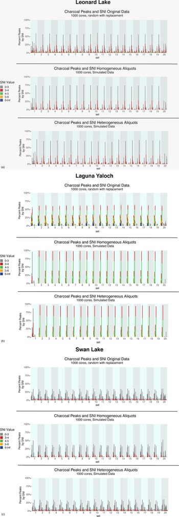
Visualizations of PEAKs detected by level, along with the associated SNI strength are shown in figures 6 a-c (A full set of tabular data are presented in Supplementary Table 4a, b). All 20 sets are shown in the figures, however discussion and interpretation of the results focuses on sets 3 to 18 in order to isolate the impact of the edge effect mentioned above. Gray bars indicate potential PEAKs that were detected but fall below the SNI threshold of 3. All other colors indicate PEAKs exceeding the threshold binned by strength.
(a–c) Bar plots showing the proportion of peaks detected (probability of detection), by level and set, for iterated CharAnalysis runs. Each level has 20,000 values, 1000 per set. Color coding indicates binned SNI strength. Calculations of percentages discussed it the text are based on 16,000 values after removal of sets 1, 2, 19, and 20 to minimize edge effects. (Figure continued on the following pages).

Original counts, random
No significant-positives occur, however insignificant-positives are common; that is, no PEAK was found in the same level in 95% of the opportunities (Table 6), although many levels show PEAKs detected >5% of the time. Leonard Lake shows 13.3% of the levels (4 of 30 levels) have insignificant-positives >5% of the time, including 24.8% of the time for level 24. Level 8 from Laguna Yaloch has the highest replicability overall, with a 60.1% PEAK detection rate. Given that these PEAKs are not detected 95% of the time, this reflects a 60.1% rate for insignificant-positives. High SNI values correspond to a large portion of the insignificant-positives at Laguna Yaloch, including for levels 4, 5, 7, and 8, for which 6–15% of the PEAKs detected had SNI of >6 (Supplementary Table 4a, b). The Swan Lake data produced the most consistent results overall with no significant-positives identified, and only level 7 produced an insignificant-positive in >5% of the opportunities.
Homogeneous Aliquots
The Leonard Lake homogeneous Poisson distributed data produced insignificant-positives in 10% of the levels, again recording 26% for level 24. Laguna Yaloch also produced insignificant-positives in 10% of the levels. Level 8 does reflect a significant-positive. Swan Lake produced insignificant-positives in 7% of the levels.
Heterogeneous Aliquots
The Leonard Lake heterogeneous Poisson distributed data produced insignificant-positives in 10% of the levels, including for 26% of opportunities in level 24. Laguna Yaloch produced insignificant-positives in 13.3% of the levels. Levels 5 and 8 have SNI values >4 for between17–60% of the PEAKs detected (Supplementary Table 4a). Swan Lake produced insignificant-positives >5% of the time in 7% of the levels.
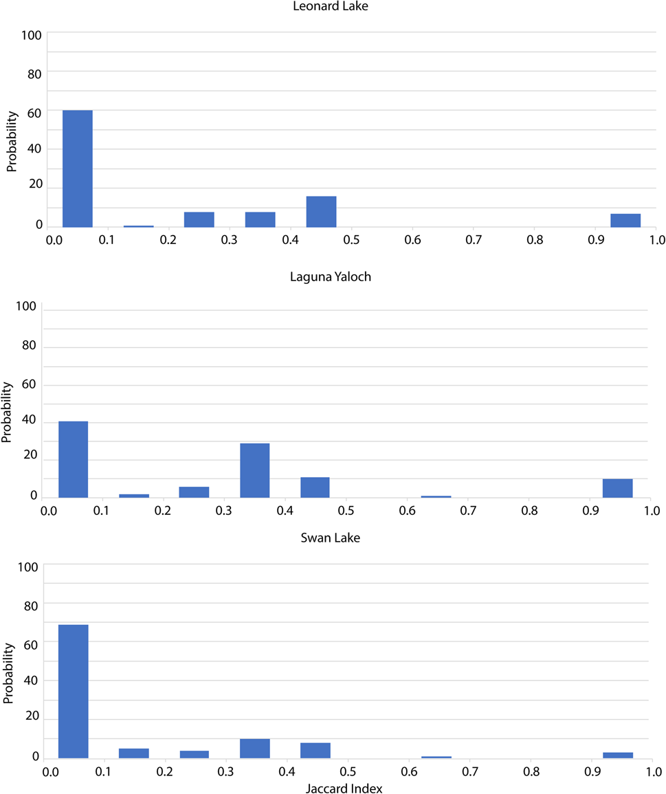
The Jaccard index for the original count data is shown in Figure 7. In all cases, there is a <10% probability of two replicate runs having a similarity index of >90%. There is an 8–15% probability of a similarity index between 40–50%. Even in the case of Laguna Yaloch, in which there is a pronounced contrast between the low and high count sections of the data and so an intuitive expectation that PEAKs would be detected consistently, there is only a 10% probability of replicate runs showing the same PEAKs.
Jaccard Index of similarity for peaks detected in 100 random with replacement runs using the original count data. The index is calculated as: $J( {X, \;Y} ) = \vert {X\mathop \cap \nolimits^ Y} \vert /\vert {X\mathop \cup \nolimits^ Y} \vert$ . An index of 1 indicates 100% similarity, while 0 indicates 0% similarity. The y-axis shows the probability of occurrence, the x-axis indicates the index values binned by 10% increments.

DISCUSSION
To our knowledge, this is the first replicate study documenting variability of intra-level charcoal count data. The range of count values found in the original data is significant. Given this, and the failure to meet the assumption of Poisson distribution, the low rate of reproducibility in CharAnalysis PEAK detection using replicated intra-level count data is not surprising. Repeated analyses of intra-level data using CharAnalysis resulted in a maximum detection rate for replicated PEAKs of 60.1%. Distribution of the Jaccard Index of Similarity showed a <10% probability of a >90% similarity. Synthetic data conforming to the assumptions of Poisson distributions produced a detection rate >95% for only one level at a single site. Increasing the threshold for the SNI does not resolve the issue. The “edge effect” observed at the beginnings and ends of the records raises significant concerns regarding “calibration” or “validation” of PEAKs detected in the most recent sections of the cores with independent records of fire. These results suggest that some assumptions explicit to the CharAnalysis algorithm are unsupported and, as a consequence, the data are being over interpreted. Moreover, this study reveals inherent limitations in charcoal particle data, which call into question the ability to detect statistically significant peaks in this type of data at all.
Of the three sites, Laguna Yaloch had the highest rate of PEAK replication. This is due to the influence of the inclusion of very high counts in the levels where peaks were identified. However, even in this instance, the large intra-level count variability restricted the overall rate of peak detection to a maximum of 61%. Leonard lake showed a probability of producing an “ephemeral” PEAK >25% of the time.
The results from the synthetic Poisson distributed data were unexpected. It is reasonable to anticipate that by meeting the statistical assumptions of the program, the detection rate of PEAKs associated with a SNI ≥3 would be >95%. Yet using Poisson distributed count values, derived from observed count means, in only one instance did the detection rate for PEAKs exceed 95% (Table 6). Insignificant-positives were identified at all three sites, in some cases at detection rates >30%, showing the high likelihood for these ephemeral peaks to be produced. Such high rates of ephemeral PEAK detection casts into question the reliability of the software, and PEAK detection methods using charcoal particle data in general.
One critique of this study could be that the data do not produce a sufficiently strong signal to be a fair test of the CharAnalysis program. However, the signal strength met or exceeded the recommended SNI threshold for all the sites. A second critique of this study might question the parameters chosen for CharAnalysis. Window width in particular could have been increased to allow for a wider range in the noise component of the interpolated data. While this could affect the presence, absence, and signal strength of the PEAKs detected, the goal of this study was to assess reproducibility based on replicated data. The evaluative component of this study is the consistency of the peak detection when replicated data are analyzed with consistent parameter settings.
Although this is not an exhaustive assessment of PEAK replicability using CharAnalysis, this study does represent a reasonable test of the algorithm's ability to reproduce results in a representative range of real-world conditions typical of those found in applications of CharAnalysis in the peer-reviewed literature. We acknowledge the imperfect fidelity of charcoal as a record of local fires, the importance of relying on multiple proxies (Whitlock et al., Reference Whitlock, Skinner, Bartlein, Minckley and Mohr2004; Higuera et al., Reference Higuera, Sprugel and Brubaker2005; Allen et al., Reference Allen, Anderson, Jass, Toney and Baisan2008; Crawford, Reference Crawford2012; Brossier et al., Reference Brossier, Oris, Finsinger, Asselin, Bergeron and Ali2014; Stivrins et al., Reference Stivrins, Aakala, Ilvonen, Pasanen, Kuuluvainen, Vasander and Gałka2019), and that more reliable results may come from systems in which charcoal influx peaks are more pronounced and obvious, such as infrequent and high-severity fires (Whitlock et al., Reference Whitlock, Skinner, Bartlein, Minckley and Mohr2004; Allen et al., Reference Allen, Anderson, Jass, Toney and Baisan2008). However, attempts to constrain paleo-fire reconstructions to studies in which past fire regimes of interest are, a priori, deemed as “appropriate” to the algorithm would require circularity in the logic of the research design.
The violation of the assumption of conformity to a Poisson distribution demonstrated here is not surprising—it has long been recognized as an issue with field data (David and Moore, Reference David and Moore1954). Overdispersion of count data most commonly arises from “clumping” (Efron, Reference Efron1986; Wilson, Reference Wilson1998). The depositional processes causing the aggregation of charcoal particles are at this point unknown. It also must be noted that variation of intra-level charcoal counts may arise from variation in experimental design and/or in sample preparation methods, although these last two factors have been controlled for in this study (see methods section). All samples from a single level were processed together, so any processing-related changes, such as breakage or disintegration, would affect all replicated samples consistently, and are therefore highly unlikely to increase the observed variance. The finding of overdispersion suggests that, at the scale of a typical sediment core, the spatial pattern of the charcoal particles may not be random. This in turn suggests conventional sampling scales are not appropriate to produce data representative of the particle population in the lake at a single level.
Another reason for divergence of the particle distribution from the Poisson assumption is likely due to the disjunct between the theoretical “depositional plane” of the lake bottom, and the actual sediment sampling resolution. If it were possible to record the pattern of particle dispersion at the time of deposition on an imaginary two-dimensional plane (i.e., the lake bottom), the particles may very well be Poisson distributed. In practical terms, however, it is all but impossible to avoid sampling across surfaces (integration of time) when subsampling sediment cores. Any thickness of sample, except in the most extreme high-sedimentation environments, integrates multiple years of deposition. As a result, all samples are likely mixed. Given the integration of time in charcoal samples, coupled with several other poorly understood processes, there is no reason to expect particle distributions to reflect a theoretical spatial pattern of deposition.
A potential resolution of this issue rests in determining the appropriate sampling scale. The clumped distribution of charcoal particles results in unpredictable heterogeneity. This problem has been examined extensively in geologic studies because it has significant implications for modeling sub-surface rock structures associated with ore deposits and oil reservoirs. Attempts to account for heterogeneity have found that the issue lies with the inability to scale distribution patterns, and hence models generally estimate uncertainty via a suite of stochastic simulations (Isaaks and Srivastava, Reference Isaaks and Srivastava1989; Anguy et al., Reference Anguy, Ehrlich, Prince, Riggert, Bernard, Yarus and Chambers1994; Armstrong, Reference Armstrong1998). Thus, the solution is determining a sample size that will accommodate the clumped pattern, such that the distribution is random at the scale of the sampling, thereby meeting the assumptions implicit in CharAnalysis. The ideal sampling scale would be (1) large enough to accommodate the clumping (returning count distributions that conform to the assumption of a Poisson distribution) and (2) still small enough to be practical given the typical size of coring devices employed.
Graduated quadrat analysis can be used to provide an empirically derived estimate of the appropriate scale needed to support the assumption of a random distribution (Wiegert, Reference Wiegert1962; Kershaw, Reference Kershaw1964; Upton and Fingleton, Reference Upton and Fingleton1989). In this method a quadrat sampling structure is used to sum progressively larger sets of successive adjacent cells. The scale at which the variance of the sets of summed samples diminishes is used to determine the appropriate sampling scale. We attempted this with the 2 × 10 grid of replicates from our cores (Supplementary Section 3; Supplementary Table 5) by combining data from two and four contiguous samples. Results from all sample volumes (1.25, 2.5, and 5.0 cc) show clumping persists. The graduated quadrat protocol recommends starting with the smallest quadrat size possible, an ideal scale resulting in ~20% zero values. Our smallest quadrat of 1.25 cc was not small enough to satisfy this criterion, and our largest quadrat was too small to capture a random distribution. Given the constraints presented by the size of sediment cores and the resolution of our sampling grid, a sampling scale appropriate to the spatial patterns of particle distribution for these lakes remains to be determined.
Although the sample volume sufficient to accommodate the observed clumping remains to be determined, it is clear that an understanding of the spatial distribution of charcoal at a range of scales across a given stratigraphic level is needed to develop appropriate sampling methodology. The use of a multi-corer, or very large diameter coring devices, may be needed to adequately capture the spatial variability of charcoal particles in sediments within a single lake. Point Pattern Analysis of gridded counts from such cores (Upton and Fingleton, Reference Upton and Fingleton1989) could help determine (1) the scale and degree of clustering, and (2) if there is a sampling area or volume that can reliably produce Poisson distributed particle counts.
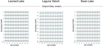
While this study shows the inherent challenges presented by charcoal particle count data to quantitative peak detection, it is also true that charcoal particle influx in sedimentary records is most certainly influenced by the proximity, intensity, and frequency of nearby fires. The theoretical assumption that background values in time series of charcoal influx represent non-local and non-fire related changes (i.e., Cback, defined as secondary transport, sediment mixing, and sediment sampling; Higuera et al., Reference Higuera, Peters, Brubaker and Gavin2007, Reference Higuera, Brubaker, Anderson, Brown, Kennedy and Hu2008) may be sound. The difficulty arises when attempting to reliably differentiate PEAK values from background and noise based on a probability. A conservative alternative is to use the straightforward method of smoothing the raw influx data. To illustrate this, we created a set of artificial cores using the random with replacement method and smoothed the data with a distance weighted mean and a 30 point (600 year) moving window (Fig. 8). Results of this analysis show CV, by level, ranging from 3.6–12.8% (Supplementary Table 6) relative to the original count data, which ranged between 9.6–91% (Supplementary Table 1). This is a simple treatment, requiring minimal manipulation of the original data. For comparison, similar analysis of the Cback values produced coefficients of variation remaining <3.9%, and not >13.3%, even in the most variable data (Supplementary Fig. 4, Supplementary Table 7), while Cpeak values were highly variable, with CV values ranging from 24% to well over 1000% (Supplementary Table 8).
Representative examples of replicated CharAnalysis runs, randomly selected, form 100 iterations of smoothed values for the Original Data: random selection, with replacement. The black line indicates the mean of all smoothed runs, the red line indicates the smoothed value of the individual run, and the gray shows the 95% probability envelope surrounding the smoothed mean for all runs. Results are shown with the x-axis indicating sets to clearly indicate the bounds of repeating sets in the artificial cores.

Given the challenges to reproducibility using the sieve and particle count method, additional charcoal quantification methods such as measuring particle area, or chemical assays such as organic biomarker analysis, should also be considered as potentially more robust methodologies.
CONCLUSIONS AND RECOMENDATIONS
Our findings show that when replicated intra-level samples are analyzed, even when the evaluative criteria for acceptance of peaks are met, the probability that CharAnalysis will identify an ephemeral peak is highly likely. We have shown that assumptions explicit in the software are unsupported in the observed data. Specifically, overdispersion analysis of intra-level charcoal count data demonstrates the assumption that charcoal is Poisson distributed spatially is violated. Greater than 90% of intra-level data failed to conform to a spatial Poisson distribution. The coefficient of variation, which provides a more intuitive sense of the degree of overdispersion in the data, is >25% in more than half of the levels analyzed. Further, the intra-level differences show a consistently high probability of being at least as large as the thresholds used to differentiate inter-level counts with low probability of coming from within the same population, although these intra-level counts originate from the same sampled level (Fig. 3a–c, Supplemental Fig. 2).
The failure of synthetic Poisson distributed data to produce consistent results suggests that, even when the assumption of Poisson distribution is met, the separation of PEAK values is an over interpretation of the data. This study shows that to have an understanding of the variability present in the charcoal particle count data from any single core, replicate counts are needed. For anything short of a full set of replicate counts of an entire core, we suggest that a qualitative interpretation is the more parsimonious use of the data.
If we accept that a signal of fire events is embedded in, though not distinguishable from, the noise component in macroscopic charcoal influx data, a more qualitative approach using smoothed influx values may provide the most robust interpretive methodology. With the luxury of replicated data, we can show the 95% probability envelope surrounding the mean of the smoothed influx values (Fig. 8). These results illustrate that “large” changes in smoothed data are necessary to have confidence that there is a significant change in charcoal input. That said, a typical macro-charcoal study lacks the replicate counts needed to make a quantitative assessment of what “large” means. It is also important to note that these data have a constant sedimentation rate associated with them, as the age model is imposed. Charcoal influx rates wholly depend on the calculations of sedimentation rates. Accurately characterizing sediment accumulation rates requires well-dated and precise age-depth modeling. As such, the estimations of sediment accumulation rates based on age-depth models introduce an additional element of uncertainty. This further emphasizes the need for conservative interpretation of changes in charcoal concentration and influx.
A final consideration for interpreting macro-charcoal influx data is the need to have sufficiently high particle counts. It is important that charcoal particle influx values be large enough to allow for meaningful differences between levels to be detected. We recommend particle concentration values be in the hundreds per cc, and careful attention be paid to how influx covaries with changing accumulation rates. Counts on the scale of tens are likely to suffer from “the small number problem” (i.e., small changes in small numbers, especially when viewed from the perspective of proportionate change, can appear to be “significant” when they may in fact fall within the random noise portion of the data variability).
The data presented here show that variability in charcoal particle count data at the scale of sediment core samples does not conform to the statistical assumptions required by CharAnalysis for quantitative reconstructions of local fire events (PEAKs) and associated fire frequencies. At all three sites, and for 98% of the levels counted, the assumption of Poisson distribution is violated. The highest rate for replicate PEAK detection was 60.1%. These findings warrant significant concern regarding the application of quantitative peak detection methodology generally. At a minimum, users need to test the requisite assumptions on a site by site basis if quantitative analysis is to be applied. Specifically, it must be shown that the intra-level count variability is less than the noise component of the time series as calculated by CharAnalysis. This requires replication of charcoal counts from within the same level. Alternatively, a parsimonious solution is to restrict interpretations to qualitative evaluation of changes in smoothed particle influx values, substantiated by independent proxy data indicative of pertinent environmental change. This treatment reduces manipulation of the data, is simple and easy to execute, and provides a means to detect qualitatively large changes in fire activity using macroscopic charcoal.
Acknowledgments
We would like to thank Marco Aquino-Lopez, Daniel Gavin, and one anonymous reviewer for their rigorous and thoughtful reviews; the manuscript is greatly improved by their input. We would also like to thank Ellie Broadman for her countless hours of microscope time, Kevin Nichols for many substantial and helpful conversations, and Jonathan Hagstrum for his constructive comments on skillful language for a broad audience. All contributed fundamentally to the quality, rigor, and accessibility of this work.
Funding
This work was supported by the USGS Climate Research and Development Program.
Supplementary Material
The supplementary material for this article can be found at https://doi.org/10.1017/qua.2022.43