Nomenclature
- FLx
-
axial component of the Lorentz force
- MHD
-
magnetohydrodynamic
- Open FOAM
-
Open Field Operation and Manipulation
- SWBLI
-
shock-wave/boundary-layer interaction
- TPS
-
thermal protection systems
Latin Symbols
- A f
-
pre-exponential factor
- B
-
magnetic induction strength
- B 0
-
magnetic field strength at the feature point
- C O
-
molar fraction of oxygen atoms
- C p
-
pressure coefficient
- C N
-
molar fraction of nitrogen atom
- C NO
-
molar fraction of nitric oxide
- C e-
-
molar fraction electron
- E
-
electric field strength
- E t
-
total energy per unit volume
- E v
-
vibro-electronic energies per unit volume
- h s
-
total enthalpy
- h ve,s
-
vibration-electron enthalpy
- J
-
electric current density
- J s,j
-
mass diffusion flux of component s in the j direction
- k b,r
-
backward reaction rate coefficient
- K eq
-
equilibrium constant
- k f,r
-
forward reaction rate coefficient
- L ref
-
radius of the cone of the vehicle
-
 $\overrightarrow m $
-
magnetic dipole angle vector
- M i
-
molecular weight of species i
- n x
-
number of grid nodes in the direction normal to the wall
- n y
-
number of grid nodes along the wall
- p
-
total pressure
- p e
-
partial pressure of the electron
- p ∞
-
freestream pressure
- q j
-
total heat conduction vector in the j direction
- q ve,j
-
the vibration-electron heat conduction vector in the j direction
- Q ve
-
vibration-electron energy source term
- r 0
-
distance from the magnetic dipole
- Rm
-
magnetic Reynolds number
-
$\overrightarrow r $
-
position vector from a point in the flow field to the centre of the magnetic dipole
- r
-
distance of the point from the centre of the magnetic dipole
- T
-
flow field temperature
- T 0
-
the reference temperature
- T a
-
temperature of activation derived from the activation energy
- T c,f
-
controlling temperature of the forward reaction
- u i
-
velocity vectors in the i directions
- u j
-
velocity vectors in the j directions
-
$\nu _{s,r}^\prime $
-
the stoichiometric coefficients of component s as reactants in reaction r
-
$\nu _{s,r}^{\prime \prime }$
-
the stoichiometric coefficients of component s as products in reaction r
- V ∞
-
freestream velocity
- y wall
-
thickness of the first layer of the grid closest to the wall


Greek Symbols
- α
-
angle between the wall and the polar axis
- αM
-
momentum adjustment coefficient
- αT
-
energy adjustment coefficient
- β
-
the temperature exponent
- γ ev
-
Joule thermal vibration energy ratio
-
${\mu _0}$
-
magnetic permeability in vacuum
- θ
-
magnetic pole angle
-
$\rho$
-
total density of the gas mixture
-
$\rho$
s
-
density of a species of s
-
${\rho _\infty }$
-
freestream density
- σ
-
electrical conductivity
- σ 0
-
reference electrical conductivity
-
${\tau _{ij}}$
-
viscous stress tensor
-
${\dot \omega _s}$
-
chemical reaction source term


1.0 Introduction
Hypersonic vehicles are generally defined as aerospace systems that are capable of sustained flight at speeds exceeding Mach 5 within the altitude range of 30 to 80 km [Reference Gülhan, Hargarten and Zurkaulen1, Reference Anderson2]. During the atmospheric flight, these vehicles are subjected to extreme conditions, including high temperatures, intense heat flux and thermochemical non-equilibrium effects [Reference Dai, Sun and Yue3–Reference Liu, Liu and Ding6]. Consequently, the development of effective thermal protection systems (TPS) has received significant attention. In recent years, advancements in superconducting materials have enabled the realisation of high-strength magnetic field devices, accelerating research into MHD TPS for advanced aerospace applications [Reference Shu, Zhong and Feng7, Reference Rashid, Zafar and Emmanual8].
Because of the potential of MHD to mitigate wall heat flux in hypersonic vehicles, extensive experimental research has been conducted. Fomichev et al. [Reference Fomichev and Yadrenkin9] experimentally observed that MHD interactions significantly alter shock wave structures. Su et al. [Reference Su, Cheng and Wang10] demonstrated through experiments that MHD flow control induces notable modifications in the aerodynamic characteristics around ramp structures. Furthermore, Borghi et al. [Reference Borghi, Carraro and Cristofolini11] found through experimental investigations that MHD interactions increase the shock standoff distance. To enhance the thermal protection effectiveness of MHD, increasing the magnetic field strength and improving the gas electrical conductivity have been shown to effectively reduce wall heat flux [Reference Gong, Li and Wang12, Reference Minkwan13].
Compared with experimental studies, numerical simulations are a safe and efficient alternative method that has garnered significant attention in recent years. In the realm of MHD research, extensive efforts have been dedicated to advancing numerical simulation techniques. For instance, Ryakhovskiy et al. [Reference Ryakhovskiy and Schmidt14, Reference Ryakhovskiy and Schmidt15] effectively utilised Open Field Operation and Manipulation (OpenFOAM) to investigate MHD interactions, developing numerical schemes that established the theoretical groundwork for future flow control applications on MHD. Korotaeva et al. [Reference Kadochnikov, Loukhovitski and Starik16] demonstrated that strong MHD interactions cause the bow shock wave to move away from the vehicle surface, thereby reducing wall heat flux. Furthermore, Bityurin et al. [Reference Bityurin and Bocharov17, Reference Bityurin, Bocharov and Popov18] provided a comprehensive analysis of the aerodynamic heating effects of MHD on the flow field, elucidated the underlying mechanisms through a series of systematic simulations.
To further investigate the relationship between aerodynamic heating effects and aerodynamic drag in MHD flow control, Li et al. [Reference Li, Liu and Liu19] revealed a negligible yet positive correlation between MHD shock control and thermal protection. However, when the boundary layer exhibits a strong Lorentz force effect and the shock standoff distance increases, the thermal protection performance can be further enhanced. Such a finding highlights the crucial role of the Lorentz force in improving thermal protection performance. As research progresses toward replicating the real gas environment of hypersonic vehicles, the issue of shock wave/turbulent boundary layer interactions induced by turbulence models has gained increasing attention [Reference Muir and Nikiforakis20, Reference Ding, Jiang and Dong21]. Additionally, Ding et al. [Reference Ding, Jiang and Gao22–Reference Ding, Liu and Jiang24] investigated the influence of MHD on vehicle control by integrating an electrical conductivity model and high-temperature gas effects, demonstrating that excessive electrical conductivity results in a thermal saturation phenomenon. The introduction of the real gas model significantly increased the thermal load of the vehicle.
Recently, the impact of the magnetic pole angle on the flow field has garnered significant attention. Nagata et al. [Reference Nagata, Otsu and Yamada25, Reference Nagata, Otsu and Yamada26] examined the force characteristics of the vehicle. The results indicated that variations in the magnetic inclination angle alter the Lorentz force distribution, disrupting the equilibrium and subsequently influencing the MHD flow characteristics. Subsequently, Nagata et al. [Reference Nagata, Yamada and Abe27] explored the effects of magnetic field inclination on complex flow structures using a double-cone configuration. The results indicated that variations in the magnetic field structure significantly affected the size of separation bubbles. Wang et al. [Reference Wang, Tian and Li28] analysed the effects of magnetic pole angle on vehicle aerodynamics from a mechanistic perspective.
The thermal protection effect of MHD has been extensively studied. However, the effects of magnetic pole angle (θ) on the flow field have been poorly understood. Specifically, the coupling of aerodynamic heating and chemical composition in the flow field under different θ is unknown. Based on the open-source software OpenFOAM and the low magnetic Reynolds number assumption, the thermochemical non-equilibrium MHD equation is introduced in the current study. A magnetic dipole model is developed, with a particular focus on quantifying the influence of θ on aerodynamic heating loads, considering non-equilibrium chemical effects. The effect of θ on shock standoff distance and particle distribution regions is analysed. The research lays a theoretical foundation for aerodynamic thermal protection in hypersonic vehicles.
2.0 Physical Model
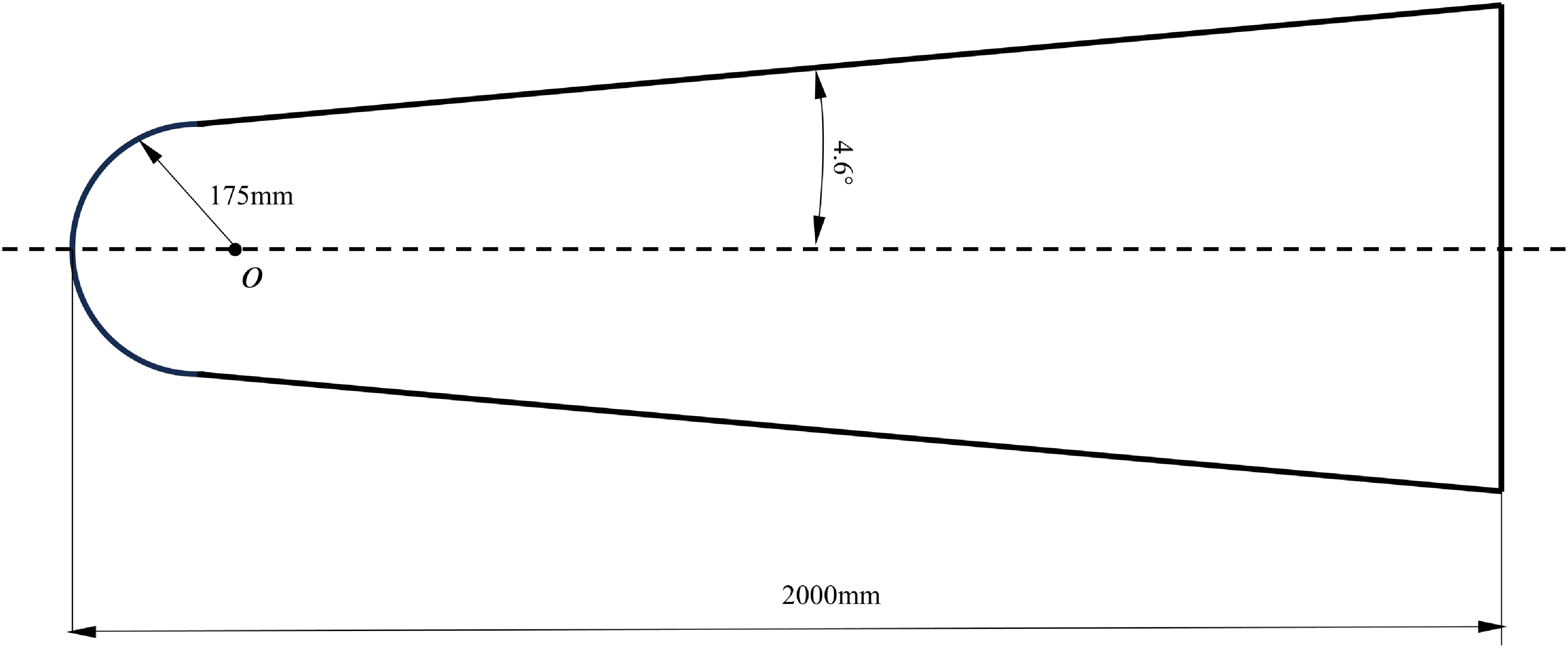
Figure 1 depicts the vehicle geometric model of ELECTRE [Reference Muylaert, Walpot and Haeuser29], which has an overall length of 2000 mm, a half-cone angle of 4.6° and a blunt head radius of 175 mm. The ELECTRE hypersonic vehicle features a blunted conical configuration. The two-dimensional axisymmetric approach is applied to determine fluid domains. Compared to a complete three-dimensional model, the two-dimensional axisymmetric structure significantly reduces the number of grid cells while preserving essential flow characteristics.
ELECTRE vehicle geometry model [Reference Fomichev and Yadrenkin9].

3.0 Numerical Method
3.1 Non-equilibrium magnetohydrodynamic equation
The governing equations in this paper are composed of thermochemical nonequilibrium coupling MHD equations. Consequently, the effect of magnetic interactions is described by incorporating a kinetic term into the momentum equation and a Joule heating term into the energy equation. The 2-dimensional axisymmetric thermochemical non-equilibrium MHD equation is derived based on the above premise. Due to the low magnetic Reynolds number (Rm << 1), the induced magnetic field can be ignored. The magnetic Reynolds number is defined by equation [Reference Nagata, Otsu and Yamada25]:
 \begin{equation}Rm = {\mu _0}\sigma {V_\infty }{L_{{\rm{ref}}}}\end{equation}
where μ 0 is magnetic permeability in vacuum, σ is electrical conductivity, V ∞ is freestream velocity, and L ref is the radius of the cone of the vehicle.
The mass, momentum, total energy, and vibrational electronic energy equations are given below as in Ref. (Reference Assonitis, Paciorri and Bonfiglioli30–Reference Luo, Wu and Chang33).
 \begin{equation}\frac{{\partial {\rho _s}}}{{\partial t}} + \frac{\partial }{{\partial {x_j}}}\left( {{\rho _s}{u_j} + {J_{s,j}}} \right) = {\dot \omega _s}\end{equation}
 \begin{equation}\frac{\partial }{{\partial t}}\left( {\rho {u_i}} \right) + \frac{\partial }{{\partial {x_j}}}\left( {\rho {u_i}{u_j} + p{\delta _{ij}} - {\tau _{ij}}} \right) = {(J \times B)_i}\end{equation}
 \begin{equation}\frac{{\partial {E_t}}}{{\partial t}} + \frac{\partial }{{\partial {x_j}}}\left( {({E_t} + p){u_j} - {\tau _{ij}}{u_i} + {q_j} + \sum\limits_{s = 1}^{ns} {{J_{s,j}}} {h_s}} \right) = J \cdot E\end{equation}
 \begin{equation}\frac{{\partial {E_{ve}}}}{{\partial t}} + \frac{\partial }{{\partial {x_j}}}\left( {{E_{ve}}{u_j} + {q_{ve,j}} + \sum\limits_{s = 1}^{ns} {{J_{s,j}}} {h_{ve,s}}} \right) + {p_e}\frac{{\partial {u_j}}}{{\partial {x_j}}} = {Q_{ve}} + {\gamma _{ev}}\frac{{J \cdot J}}{\sigma }\end{equation}
where
 $\rho$
s
represents the density of a species of s. u
i
and u
j
are velocity vectors in the i and j directions, respectively. p is the total pressure, and p
e
is the partial pressure of the electron. The total and vibro-electronic energies per unit volume are denoted as E
t
and E
ve
, respectively. J
s,j
is the mass diffusion flux of component s in the j direction.
 ${\dot \omega _s}$
is the source term of the chemical reactions.
 ${\tau _{ij}}$
is the viscous shear tensor. q
j
and q
ve,j
represent the total heat conduction vector and the vibration-electron heat conduction vector in the j direction, respectively. B is the magnetic field strength. Total enthalpy and vibration-electron enthalpy are expressed by h
s
and h
ve,s
, respectively. Q
ve
is the vibration-electron energy source term. (J × B)
i
represents the Lorentz force, J·E, and γ
ev
(J·J)/σ represents Joule heat, and J is the current density. The parameter γ
ev
represents the Joule thermal vibration energy ratio.
σ is the electrical conductivity of the plasma. The surface material is assumed to be entirely insulated, and the Hall effect is disregarded for simplicity. According to the Ohm’s law, the current can be calculated by the following Equation (6) [Reference Nagata, Otsu and Yamada25].
 \begin{equation}J = \sigma (E + u \times B)\end{equation}
The chemical reaction source term
 ${\dot \omega _s}$
is given by Equation (8) [Reference Yang and Liu34]:
 \begin{equation}{\dot \omega _{\rm{s}}} = {{\mathop{{\textit {M}}}\nolimits} _{\rm{s}}}\sum\limits_{r = 1}^{nr} {\left( {\nu _{s,r}^{\prime \prime } - \nu _{s,r}^\prime } \right)} \left[ {{{\mathop{\rm k}\nolimits} _{f,r}}\prod\limits_{{\rm{i}} = 1}^{n{\rm{i}}} {{{\left( {\frac{{{\rho _{\rm{s}}}}}{{{{\mathop{{\textit {M}}}\nolimits} _{\rm{s}}}}}} \right)}^{\nu _{s,r}^\prime }}} - {{\mathop{\rm k}\nolimits} _{b,r}}\prod\limits_{{\rm{i}} = 1}^{n{\rm{i}}} {{{\left( {\frac{{{\rho _s}}}{{{{\mathop{{\textit {M}}}\nolimits} _{\rm{s}}}}}} \right)}^{\nu _{s,r}^{\prime \prime }}}} } \right]\end{equation}
where
 $\nu _{s,r}^{\prime \prime }$
and
 $\nu _{s,r}^\prime $
are the stoichiometric coefficients of component s as products and reactants in reaction r, respectively. M
s
is the molecular weight of species s. The Park 93 species-7 [Reference Park35] component reaction model is used to simulate the chemical processes in the aforementioned framework. This model primarily consists of the dissociation reaction of N2 and O2, the exchange reaction that produces NO, and the ionisation reaction that generates NO+ and e−.
The forward reaction rate coefficient k f,r is determined by Arrhenius formulas as [Reference Casseau, Palharini and Scanlon36]:
 \begin{equation}{{{k}}_{{{f,r}}}}{{ = }}{{{A}}_{{f}}} \times {{T}}_{{{c,f}}}^{{b}}\exp \bigg ({{ - }}\frac{{{{{T}}_{{a}}}}}{{{{{T}}_{{{c,f}}}}}}\bigg)\end{equation}
where A f is a pre-exponential factor, β is the temperature exponent, and T a is the temperature of activation derived from the activation energy. T c,f is the controlling temperature of the forward reaction.
Park et al. [Reference Zhang, W37] chose a least-squares curve fit of the equilibrium constant K eq to calculate k b,r [Reference Yang and Liu34]. The backward reaction rate coefficient k b,r can be calculated by the following formula:
 \begin{equation}{{\mathop{ k}\nolimits} _{b,r}} = \frac{{{k_f}}}{{{K_{eq}}}}\end{equation}
where T a is the activation temperature, T c,f = T tr 0.7 T ve 0.3, and K eq is the equilibrium constant (dimensionless) calculated by a function of temperature based on the curve-fitted method.
 \begin{equation}K_{\mathrm{eq}} = \exp \left[ a_1 \left( \frac{T}{10000} \right) + a_2 + a_3 \ln \left( \frac{10000}{T} \right) + a_4 \left( \frac{10000}{T} \right) + a_5 \left( \frac{10000}{T} \right)^2 \right]\end{equation}
where a 1, a 2, a 3, a 4 and a 5 are the curve fit coefficients.
Bush [Reference Nagata, Otsu and Yamada25] provided a semi-empirical electrical conductivity formula in the form of a temperature fit based on the reference electrical conductivity and the reference temperature:
 \begin{equation}\sigma = {\sigma _0}{\bigg(\frac{{{T}}}{{{{{T}}_0}}}\bigg)^n}\end{equation}
where T 0 is the reference temperature, T is the flow field temperature, and σ 0 is the reference electrical conductivity.
The electrical conductivity reference values used in this paper are consistent with those in Ref. (Reference Nagata, Otsu and Yamada25). The reference parameters are: σ 0 = 250 S·m−1, T 0 = 25000 K, and n = 2.
The computational schematic for the thermochemistry nonequilibrium MHD is shown in Fig. 2. The transport mixing rule is set by Wilke [Reference Candler38], and the multispecies transport model is Fick [Reference Kim, Kang and Park39]. The simulation starts with flow field initialisation, using initial conditions and applied transport and thermophysical properties. Subsequently, the initial conditions (such as ρ, u, T, etc.) are assigned to each grid cell. In the main solver, real gas effects are accounted for by introducing chemical reaction source terms into the continuity equation. Meanwhile, the momentum, total energy and vibrational energy equations are augmented with the Lorentz force, Joule heating, and vibrational energy source terms, respectively.
Computational schematic for thermochemical nonequilibrium MHD.

3.2. Magnetic dipole field
The magnetic dipole field represents the magnetic field generated by a closed loop, which can be compared to the energised solenoid model. The magnetic dipole field distribution can be derived from the magnetic field strength at the feature points [Reference Ding, Jiang and Dong23, Reference Nagata, Otsu and Yamada26]:
 \begin{equation}\overrightarrow B = - \frac{{{B_0}}}{{2{{(r/{r_0})}^3}{r^2}}}\left( {3\overrightarrow r (\overrightarrow r \cdot \overrightarrow m ) - {r^2}\overrightarrow m } \right)\end{equation}
where B
0 represents the magnitude of magnetic induction strength at the characteristic point. r
0 denotes the distance of the feature point from the centre of the magnetic dipole and is assumed to be 175 mm here.
 $\overrightarrow r $
denotes the position vector from a point in the flow field to the centre of the magnetic dipole. r is the distance of the point from the centre of the magnetic dipole and
 $\overrightarrow m $
represents the vector denoting the angle of the magnetic dipole.
Assuming the magnetic dipole is centred at (x
0, y
0, z
0). The magnetic dipole angle (
 $\theta $
) is rotating counterclockwise around the Z-axis along the central position axis. The vectors
 $\overrightarrow m $
and
 $\overrightarrow r $
are expressed as:
 \begin{equation}\overrightarrow m = \left[ \begin{array}{l}\cos \theta \\{\rm{sin}}\,\theta \\0\end{array} \right]{\rm{ }}\overrightarrow r = \left[ \begin{array}{l}x - {x_0}\\y - {y_0}\\z - {z_0}\end{array} \right]\end{equation}
The magnetic field distribution of a magnetic dipole is centred at (x 0, y 0, z 0) rotating around the Z-axis in the Cartesian coordinate system:
 \begin{equation}\left[ \begin{array}{l}{B_x}\\{B_y}\\{B_z}\end{array} \right] = - \frac{{{B_0}}}{{2{{(r/{r_0})}^3}{r^2}}}\left[ \begin{array}{c}2{(x - {x_0})^2}\cos \theta - {(y - {y_0})^2}\cos \theta - {(z - {z_0})^2}\cos \theta + 3(x - {x_0})(y - {y_0})\sin \theta \\[5pt]2{(y - {y_0})^2}\sin \theta - {(x - {x_0})^2}\sin \theta - {(z - {z_0})^2}\sin \theta + 3(x - {x_0})(y - {y_0})\cos \theta \\3(x - {x_0})(z - {z_0})\cos \theta + 3(y - {y_0})(z - {z_0})\sin \theta \end{array} \right]\end{equation}
The spatial magnetic field distribution of the model is shown in Fig. 3 [Reference Nagata, Otsu and Yamada26]. The magnetic field strength at point P is B 0 and the distance from the magnetic dipole is r 0. Point P is a feature point for the magnitude of the magnetic field strength.
Schematic of dipole magnetic field distribution [Reference Nagata, Otsu and Yamada26].

Figure 4 illustrates the distribution of the magnetic field in the meridional plane for three angular configurations (θ = 0°, 45°, and 90°). Since other magnetic pole angles are similar to 45°, only three typical distributions of magnetic inductances are shown here. The electromagnetic coil is approximated as an idealised magnetic dipole aligned with the body axis for analytical clarity. The effects of MHD interactions are systematically analysed by varying θ (θ = 0°, 30°, 45°, 60° and 90°) between the vehicle axis and the applied dipole field orientation. The uniform magnetic field strength of B 0 = 4 T is used for all simulations.
Diagram of the magnetic field with different pole angles.

3.3 Boundary conditions
As practiced in Ref. (Reference Zhang, Wang and Zhang40), the boundary conditions for vehicles are established. At 293 seconds, the ELECTRE [Reference Muylaert, Walpot and Haeuser29] vehicle is flying at a velocity of 4230 m·s−1 at an altitude of 53.3 km. The atmosphere temperature is 265 K, pressure is 52.8 Pa, viscosity is 1.68 × 10⁻⁵ (kg·(m/s)−1) and density is 6.9 × 10⁻⁴ (kg/m3) [41]. The atmosphere composition consists of 22% O2 and 78% N2. The wall boundary conditions are applied without considering catalytic effects.
The computational domain is meshed based on the physical model presented in Section 2. A structured grid is employed to enhance convergence speed and improve computational accuracy. To precisely capture heat flux through the vehicle walls, the boundary layer grid is refined layer by layer. In accordance with the OpenFOAM solver framework, the axisymmetric computational domain is reformulated as a wedge-shaped structure. Figure 5 illustrates the grid structure of the fluid domain.
ELECTRE vehicle boundary and grid model.

3.4 Code verification
The Hy2Foam solver, a density-based, compressible, non-equilibrium flow solver built on the OpenFOAM platform, was developed at Strathclyde University [Reference Casseau, Palharini and Scanlon36, Reference Zhang, Zhang and Yang42]. The magnetic dipole field is further integrated into the hy2Foam framework, forming the foundation for the subsequent research conducted in this study. The current study configures the solver with a maximum Courant number of 0.7.
Based on the RAM-C blunt cone model [Reference Ding, Jiang and Dong23], this section verifies the accuracy of the numerical model of thermochemical non-equilibrium MHD and the accuracy of the electrical conductivity model in this paper. The total length of the RAM-C blunt cone model is 1.295 m, the radius of the head is 0.1524 m and the angle between the cone and the central axis is 9°.
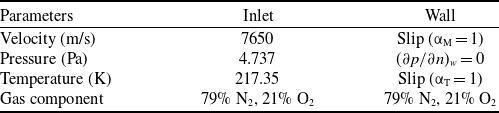
The flight altitude of the RAM-C blunt cone model is 71 km, and the speed is 7650 m/s. The specific boundary conditions are set in Table 1. The static pressure, static temperature and dynamic viscosity of the freestream are 4.737 Pa, 217.35 K and 1.4377 × 10⁻⁵ (kg·(m/s)−1), respectively. The Reynolds number of the freestream is 12316. The wall is set slip with complete diffuse reflection. The momentum adjustment coefficient (αM) is 1.0, the energy adjustment coefficient (αT) is 1.0, and the wall temperature is 1500 K. The wall catalytic reaction is not considered. The magnetic field distribution is consistent with Ref. (Reference Nagata, Otsu and Yamada26), where the magnetic field is a dipole field. The centre of the magnetic dipole overlaps with the center of the head of the RAM-C blunt cone. The magnetic field strength at the feature point is B 0 = 0.5 T, and the distance between the feature point and the magnetic dipole center is r 0 = 0.1524 m.
RAM-C blunt cone boundary conditions

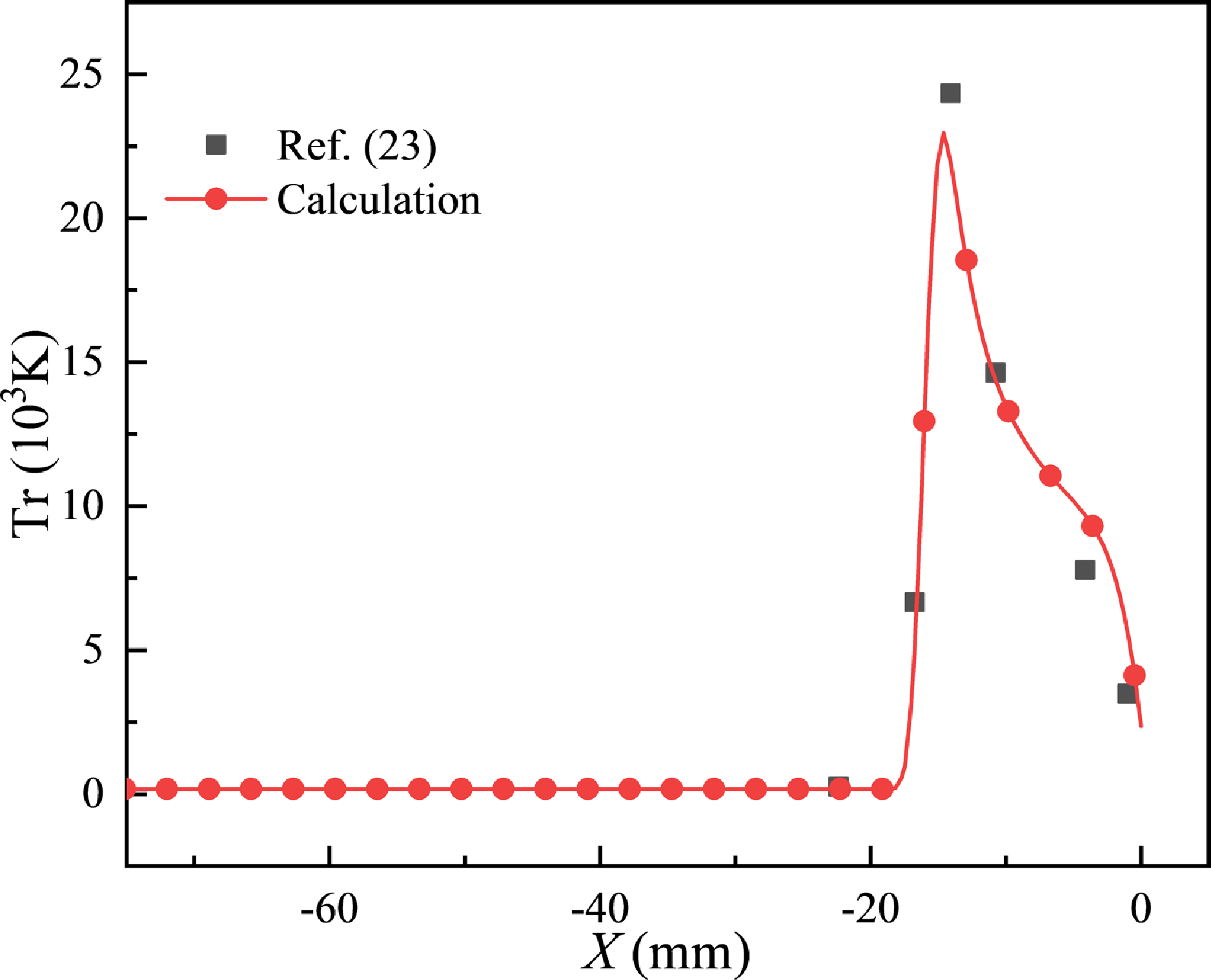
Figure 6 shows the validation of the trans-rotational temperature curve for the RAM-C vehicle along the stagnation point line. As shown in Fig. 6, the trans-rotational temperature and shock standoff distance calculated in this study agree well with the results reported in Ref. (Reference Ding, Jiang and Dong23).
Case validation of MHD.

3.5 Grid independence
Following the grid generation methodology established in Ref. (Reference Zhang, Zhang and Yang42), the grid convergence study is conducted using three different grid numbers, as shown in Table 2. The terms n x , n y and y wall refer to the number of grid nodes in the direction normal to the wall, the number of grid nodes along the wall, and the thickness of the first layer of the grid closest to the wall, respectively [Reference Zhang, Zhang and Yang42]. The thickness of the grid at the location near the wall decreases from Coarse to Fine, and the number of grids rises.
Parameters for different grid sizes

Wall heat flux predictions from three grid resolutions are compared in Fig. 7. The spatial distribution of the wall heat flux is characterised using polar coordinates, where the origin coincides with the geometric centre of the vehicle (point O in Fig. 2) and the polar axis aligns with the stagnation point line. The position of the wall with respect to the polar axis is defined by the angular coordinate α. Grid resolution demonstrates a significant influence on heat flux distribution characteristics. Sensitivity to grid parameters diminishes with grid refinement, both through increased cell count and reduced first-layer thickness. The Medium grid produces wall heat flux distributions that closely match those of the Fine. Despite a 70% reduction in grid cells, the spacing of the first layer increased by 50% (as shown in Table 2). Considering the balance between computational efficiency and numerical accuracy, the medium-resolution grid is adopted for all subsequent simulations.
Verification of grid independence. (a) Wall heat flux, and (b) wall heat flux at the blunt position.

The experimental study of ELECTRE [Reference Muylaert, Walpot and Haeuser29] has been selected to validate the solver. A comparison between the calculated wall heat flux and the reference data is shown in Fig. 7. Overall, the computed wall heat flux agrees well with the experimentally measured results. Notably, at the stagnation point position, the predicted values show good agreement with the experimental values, as shown in Fig. 7(b). However, a discrepancy exists where the experimental values of wall heat flux surpass those of the prediction at the shoulder location. Such deviation may be because the wall catalysed is ignored [Reference Zhang, Zhang and Yang42]. Therefore, the validated code forms a reliable foundation for subsequent hypersonic MHD numerical simulations.
A domain independence study is conducted to ensure that the computational domain is sufficiently large to accurately capture the shock wave. The optimal computational domain size is determined by evaluating different domain sizes and comparing the resulting shock wave positions. Figure 8 presents the shock wave positions for various domain configurations.
Mach number distribution under different fluid domains.

In Case 1, the grid configuration from Section 3.5 is used, with a magnetic field strength of 4 T and a magnetic pole angle of 0°. Case 2 expands the fluid domain by a factor of 1.6 in the axial direction and 1.35 in the radial direction compared to Case 1. Similarly, Case 3 expands the fluid domain by a factor of 2 in the axial direction and 1.5 in the radial direction. Apart from mesh resolution, Cases 2 and 3 maintain the same conditions as Case 1.
As shown in Fig. 8, variations in the fluid domain have an insignificant impact on the computed results. In particular, the predicted shock standoff distance remains nearly consistent. This confirms that the computational domain of Case 1 is sufficient for accurately capturing the shock wave.
4.0 Results and Discussion
Section 3 validates the accuracy of the magnetic field, electrical conductivity model and thermochemical non-equilibrium MHD equation. The present section investigates the influence of magnetic pole angle (θ) on aerodynamic heating and forces acting on the vehicle. Additionally, the influence of θ on the shock standoff distance is elucidated, and the effect of the change of the shock wave position on the ionisation region of the gas is investigated.
4.1 Wall heat flux
Figure 9(a) shows a comparative analysis of wall heat flux distributions under five angular configurations (θ = 0°, 30°, 45°, 60°, 90°). The wall heat flux distribution reveals that the peak heat flux in the stagnation point region is declined along the blunt cone surface at θ = 0°. The maximum heat flux at the stagnation point can be attributed to the conversion of kinetic energy into thermal energy by the bow shock wave in this region. With the increasing of α, the compression effect of the bow shock wave is gradually weakened, and the wall heat flux is gradually reduced. Such a trend corroborates with hypersonic blunt cone heating characteristics reported in Ref. (Reference Kadochnikov, Loukhovitski and Starik16). Under inclination magnetic field conditions (θ = 30°, 45°, and 60°), the wall heat flux exhibits non-monotonic variation with θ, with the heat peaking (max ≈ 400 kW/m2) at α = 20° ± 2°. The inclination dipole orientation induces 35%40% aerodynamic heating load redistribution from the blunt nose region (α < 10°) to the shoulder (α = 15°-25°), demonstrating significant wall heat flux restructuring. When the magnetic pole angle is 30°, 45°, 60° and 90°, the heat flux at the surface of the blunt cone (α = 30°-110°) is higher than that at θ = 0°. The heat flux is gradually transferred from the nose to the conical part due to the magnetic pole angle action.
Distribution of heat flux with different magnetic pole angles. (a) Wall heat flux distribution, and (b) stagnation point heat flux.

Stagnation point heat flux strongly depends on magnetic pole angle: 587 kW/m² (θ = 0°), 341 kW/m² (θ = 30°), 291 kW/m² (θ = 45°), 270 kW/m² (θ = 60°), and 611 kW/m² (θ = 90°), forming a U-shaped distribution with a minimum at θ = 60°, as shown in Fig. 9(b). Relative to the θ = 0°, stagnation point heat flux levels are decreased to 58.1% (θ = 30°), 59.5% (θ = 45°) and 45.9% (θ = 60°) before increasing to 109.7% at θ = 90°. The heat flux at the stagnation point shows a non-monotonic correlation with θ. By optimising the magnetic pole angle, the maximum thermal load at the stagnation point can be reduced by 45%. When the magnetic pole angle (θ) is set to 60°, the vehicle achieves an optimal aerodynamic thermal environment. The optimal magnetic pole angle of the current work is different from that reported in Ref. (Reference Nagata, Yamada and Abe27). Ref. (Reference Nagata, Yamada and Abe27) examines a double-cone model featuring complex shock wave/turbulent boundary layer interactions at the triple point that is different from the cone structure in this paper. The external flow field of the blunt cone configuration has insignificant shock-wave/boundary-layer interaction (SWBLI) effects, which also accounts for the discrepancy between the optimal magnetic pole angle in this study and that reported in Ref. (Reference Nagata, Yamada and Abe27).
4.2 Mach number and shock standoff distance
Figure 10 shows the Mach number distribution for five magnetic pole angle conditions (θ = 0°, 30°, 45°, 60° and 90°). In the flow field, the shock wave is nearest to the wall surface at the blunt region, where the gas experiences the maximum compression. As the gas flows towards the blunt cone of the vehicle, the boundary layer is thickened and the pressure gradient is decreased. The boundary layer changes account for the lower heat flux at the blunt cone position (compared with that at the blunt nose position) in Fig. 9.
Contour of Mach number with different magnetic pole angles.

Figure 11(a) shows the distribution of Mach number along the stagnation point line under different θ. A subsonic zone (Mach number < 0.8) is observed in the stagnation point region at the vehicle head. Such a flow field profile agrees with Ref. (Reference Yang and Liu34). When θ = 0°, the shock standoff distance is 35.5 mm. For θ = 30°, 45°, 60° and 90°, the shock standoff distances are 35.6 mm, 34.4 mm, 29.5 mm and 18.8 mm, respectively. These values correspond to 106%, 103%, 88% and 56% of the shock standoff distance observed at θ = 0°. The shock standoff distance reaches the peak value at θ = 30°, as illustrated in Fig. 11(b).
Mach number distribution and shock standoff distance with different magnetic pole angles. (a) Mach number distribution along the stagnation point line, and (b) the shock standoff distance.

4.3 Lorentz force
Since plasma is formed around hypersonic vehicles, the Lorentz force is generated under the action of the magnetic field [Reference Nagata, Otsu and Yamada26]. Figure 12 compares Lorentz force distribution under varying magnetic pole angle conditions (θ = 0°, 30°, 45°, 60° and 90°), revealing a pronounced shift in force localisation with θ. As θ increases, the migration of the Lorentz force peak and the evolution of the shock wave morphology are observed. The magnetic flux at the shoulder position gradually increases, and the location of the peak Lorentz force moves towards the shoulder. Simultaneously, the gas ionisation region within the shock layer is evolved in response to these shock wave alterations. Consistent with Ref. (Reference Ding, Jiang and Dong23), the Lorentz force is dominantly concentrated in the head and shoulders of the vehicle.
Contour of the Lorentz force with different magnetic pole angles.

Figure 13 illustrates the X-direction components of the Lorentz force (FLx) along the stagnation point line. The spatial correspondence between the peak Lorentz force location and the shockwave standoff distance demonstrates a direct relationship with the local gas thermodynamics. The gas temperature in the shock layer is high, leading to a significant degree of ionisation. As a result, the electrical conductivity of this region is high. Based on the expression F = σu × B × B, an increase in electrical conductivity leads to a stronger Lorentz force.
Lorentz force distribution profile along the stagnation point line with different magnetic pole angles.

4.4 Pressure coefficient
The wall pressure distribution is nondimensionalised using the pressure coefficient (Cp), defined as:
 \begin{align}Cp = \frac{{p - p{}_\infty }}{{0.5{\rho _\infty }{V_\infty }^2}}\end{align}
where p is pressure,
 $p{}_\infty $
,
 ${\rho _\infty }$
, and
 ${V_\infty }$
are freestream pressure, freestream density, and freestream velocity, respectively. According to Ref. (Reference Nagata, Otsu and Yamada25), the axial force is nondimensionalised, and the pressure coefficient is obtained using similarity theory. The nondimensionalised parameter enables direct comparison of aerodynamic loading characteristics across different flight regimes.
Figure 14 illustrates the pressure coefficient (Cp) distribution profile along the vehicle surface. A monotonic pressure decline is observed from the stagnation point to the blunt-nosed cone region. The pressure maximums are exhibited at the nose region (Cp ≈ 1.8), and the environmental pressure is at the blunt cone (Cp ≈ 0.05). At the blunt nose region (0° < α < 30°), the wall pressure distribution is negligibly affected by θ. The wall pressure exhibits a positive correlation with θ elevation in the shoulder region (40° < α < 80°). The Lorentz force at the shoulder position gradually increases with θ. Simultaneously, the normal reaction force exerted by the shock wave on the wall is enhanced as the Y-direction component of the Lorentz force is strengthened. Beyond α = 80°, pressure variations are diminished significantly as MHD effects gradually weaken.
Wall distribution profile of C p with different magnetic pole angles.

4.5 Gas component
4.5.1 Mole fraction of oxygen atoms
Figure 15 shows the molar fraction distribution of oxygen atoms (C O). Accumulation of oxygen atoms is observed within the boundary layer near the vehicle wall. Under thermodynamic conditions, oxygen promotes oxygen dissociation (O2 → 2O) through endothermic reactions and results in broader spatial coverage compared to other diatomic species [Reference Anderson2, Reference Hao, Wang and Lee5]. The obtained distribution pattern qualitatively agrees with numerical predictions in Ref. (Reference Yang, Li and Xiao4). The range of oxygen atoms obtained in this paper is more extensive than that reported in Ref. (Reference Yang, Li and Xiao4). Such discrepancy is attributed to the action of MHD effects, where the shock wave is pushed by Lorentz force (J × B) and the oxygen dissociation zone is expanded. The distribution of oxygen atoms is primarily concentrated near the wall, as shown in Fig. 15. At θ = 30°, the dissociation of oxygen molecules is enhanced in the shoulder region of the vehicle. Since the C O contours under other θ conditions are similar to those in Fig. 15(b), other contours are omitted here for brevity.
Contour of the molar fraction of oxygen atoms with different magnetic pole angles.

Figure 16 examines the C O profile along the stagnation point line with varying θ, elucidating the influence of θ on oxygen dissociation. A non-monotonic variation in oxygen atom spatial distribution is observed, which is characterised by an initial increase, reaching a peak θ = 30° and a decrease afterwards. The maximum distribution range (X ≈ 35.5 mm) occurs at θ = 30°, corresponding to the shock standoff distance. When θ exceeds 45°, the concentration range of oxygen atoms is gradually decreased, and the minimum is reached at θ = 90°. As shown in Fig. 10, the distribution of oxygen atoms is closely correlated with the shock standoff distance, as the shock wave position is dictated by the boundary layer thickness and influences the oxygen dissociation.
Molar fraction of oxygen atoms profiles along the stagnation point line with different magnetic pole angles.

The control of the Lorentz force distribution ( F = σu ×B×B) is facilitated by the variation of θ, as demonstrated in Ref. (Reference Wang, Tian and Li28). The oxygen dissociation range reaches a peak and then gradually decreases as θ increases. At θ = 30°, the dissociation enhancement is maximised, effectively reducing stagnation point heat flux by utilising endothermic reaction energy.
4.5.2 Mole fraction of nitrogen atoms
The dissociation of nitrogen molecules into individual nitrogen atoms requires substantial energy [Reference Anderson2]. The molar fraction of nitrogen atoms (C N) is a key critical parameter for stagnation point heat flux prediction. Figure 17 shows the C N contour under different θ. Since the C N contours under other θ conditions are similar to those shown in Fig. 18(b), the other contours are not shown again for brevity. A pronounced accumulation of nitrogen atoms is observed in the stagnation point region and the shoulder. Due to the significant bond dissociation energy disparity between N2 (941 kJ/mol) and O2 (498 kJ/mol), the C N is two orders of magnitude lower than C O. As θ increases, the number of nitrogen atoms in the head region gradually decreases as the nitrogen atoms at the shoulder are transported to the blunt cone. The ionisation region of the gas in the shock layer is changed in response to changes in the shock wave position.
Contour of the molar fraction of nitrogen atoms with different magnetic pole angles.

Molar fraction of nitrogen atoms profiles along the stagnation point line with different magnetic pole angles.

Figure 18 shows the C N profile along the stagnation point line. The distribution of nitrogen atoms is similar to the results reported in Ref. (Reference Yang, Li and Xiao4). Compared to Ref. (Reference Yang, Li and Xiao4), the distribution of nitrogen dissociation is enhanced through the Lorentz force by MHD. Double peak C N distribution emerges (primary peak at X ≈ 6 mm and secondary at X ≈ 30 mm) along the stagnation point line. An additional peak is caused by the MHD effects, as the Lorentz force drives the outward extension of the shock wave. A secondary ionisation region is formed outside the shock wave layer accordingly.
The peak and concentration range of nitrogen atoms are affected by the change of the θ. At θ = 30°, the shock standoff distance reaches its maximum while the gas pressure gradient in the boundary layer is minimised. The range of nitrogen atoms at the stagnation point is increased by 16.7% compared to that at θ = 0°. When θ ≥ 45°, the distribution range of nitrogen atoms is reduced due to the thinning of the boundary layer. In other words, boundary layer expansion can be induced by a sufficiently strong Lorentz force, thereby increasing the dissociation range of nitrogen.
4.5.3 Mole fraction of nitric oxide atoms
Figure 19 characterises the mole fraction of nitric oxide (C NO). The nitric oxide is mainly distributed in the stagnation point zone and the conical surface. When T = 2500 – 9000 K, the production threshold of NO is reached, following the Arrhenius kinetics [Reference Anderson2]. The results indicate that nitric oxide production depends on the molar concentration of nitrogen atoms, as shown in Figs 14 and 16. At a magnetic pole angle of θ = 30°, the concentration range of nitric oxide along the stagnation point line is widened by increasing the shock standoff distance. For θ > 45°, the axial projection of the Lorentz force is reduced, as indicated by MHD vector analysis in Ref. (Reference Su, Cheng and Wang10), leading to a contraction of the nitric oxide distribution in the blunt nose region. Under other θ conditions, the C NO contours are similar to those in Fig. 19(c) and are not presented again here.
Contour of the molar fraction of nitric oxide with different magnetic pole angles.

Figure 20 further compares the nitric oxide profile along the stagnation point line across different θ. When θ = 0°, the pattern of the nitric oxide profile is similar to those reported in Ref. (Reference Yang, Li and Xiao4). Compared to Ref. (Reference Yang, Li and Xiao4), the dissociation region in the present study is enlarged due to the effects of MHD. The nitric oxide is primarily localised within the thermochemical boundary layer between the shock wave and the vehicle surface. The shock wave is extrapolated by MHD. The residence time of the particles is prolonged by the increased shock standoff distance, which causes the concentration of nitric oxide to increase.
Molar fraction of nitric oxide profile along the stagnation point line with different magnetic pole angles.

The distribution range of nitric oxide along the stagnation point line changes with the shock position due to the change of the parameter θ. The distribution of C
NO under the Lorentz force reaches a maximum (30 mm) at θ = 30°, an 8 mm increase compared to θ = 0°. At θ = 30°, the peak normal force of the Lorentz force is observed, consistent with Ref. (Reference Nagata, Otsu and Yamada26). Optimising θ reduces the near wall C
NO gradient by 41% (
 $\nabla {C_{{\rm{NO}}}}\,:\, 0.0295 \rightarrow 0.0217 {{\rm{mm}}^{-1}}$
) and concurrently suppresses the surface recombination effect.
4.5.4 Mole fraction of electrons
Figure 21 shows the molar fraction of electrons (C e−) contour. A significant accumulation of electrons is observed in the stagnation point zone, consistent with Ref. (Reference Fomichev and Yadrenkin9). Despite minor discrepancies arising from geometric scaling and Mach number variations, the distribution profile is in agreement with Ref. (Reference Yang and Liu34). The majority of electrons remain in the stagnation point, while a smaller fraction appears near the vehicle shoulder. Figure 21 highlights the significant change in the concentration of electrons in the flow field as θ increases to 30°. Under other θ conditions, the C e− contours are similar to those shown in Fig. 21(b) and are therefore not presented here.
Contour of the molar fraction of electrons with different magnetic pole angles.

Figure 22 illustrates the distribution of C e− for as a function of θ. The electrons on the stagnation point line exhibit non-monotonic behaviour, reaching maximum ionisation intensity at θ = 30° and minimum at θ = 90°. The Lorentz force is affected by θ, causing variations in both magnitude and orientation. As the shock wave shifts, the ionisation region of the gas is affected in response to the dynamic interactions. For θ < 45°, the ionisation region is extended by 4 mm and 1 mm beyond the θ = 0° case, a consequence of the increased shock standoff distance. Conversely, for θ ≥ 45°, the ionisation region is contracted by 4.4 mm and 13.9 mm. A similar pattern is reported in Ref. (Reference Nagata, Otsu and Yamada26). The reduction in the shock layer thickness for θ > 45° suggests a concurrent decrease in the ionisation region. A comparison with Fig. 10 indicates that the shock standoff distance and ionisation region exhibit a similar pattern. Gas ionisation primarily occurs within the bow shock layer, where the high-temperature gas is compressed.
Molar fraction of electrons profile along the stagnation point line with different magnetic pole angles.

The C e− exhibits the lowest concentration among all plasma due to the thermochemical sequencing: O2/N2dissociation (T > 2500 K) → radical recombination (T > 4500 K) → thermal ionisation (T > 9000 K) [Reference Anderson2]. The ionisation threshold (T = 9015 ± 230 K) [Reference Anderson2] exceeds dissociation temperatures (T = 2540 K for O2, 7030 K for N2) by 255-1985 K. As a result, electron concentrations remain 1–2 orders of magnitude lower than C O and C N levels [Reference Anderson2]. The electron density peak (C e− max = 0.03 %) occurs at the same position of the shock wave peak (as shown in Fig. 9). Since the gas pressure and temperature in the shock layer are at the highest, the degree of ionisation and electrical conductivity are at the maximum.
5.0 Conclusion
This study employs the nonequilibrium Navier-Stokes equations to resolve thermochemical nonequilibrium reactions and gas-phase interactions occurring on the vehicle surface for the low magnetic Reynolds number conditions. The influence of gas composition, thermal protection effects and aerodynamic characteristics of the flow field is analysed by varying the magnetic field angle. The main conclusion includes:
-
(1) The shock standoff distance initially increases, then decreases with the rising θ. At θ = 30°, the maximum shock standoff distance is reached, increased by 6% compared to that from the θ = 0° case. In contrast, the wall heat flux at θ = 60° is reduced to 46% of that from the θ = 0° case, indicating significant thermal attenuation.
-
(2) The shock characteristics of the flow field are greatly affected by θ, and the shock standoff distance reaches a peak when θ = 30°. The peak position of the Lorentz force in the X direction is highly consistent with the shock standoff distance. Meanwhile, the Y-component of the Lorentz force plays a crucial role in the wall pressure on the vehicle shoulder. As θ increases, the wall pressure on the shoulder of the vehicle exhibits an increasing trend.
-
(3) The distribution characteristics of nitric oxide and oxygen atoms exhibit identical single peak profiles, whereas nitrogen atoms and electrons show significant bimodal characteristics. The θ parameter maintains the fundamental distribution morphology of ions and molecular species while primarily governing the particle distribution region. The distribution of gas dissociation positively correlates with the shock standoff distance. The distribution of oxygen atoms, nitrogen atoms, nitric oxides and electrons along the stagnation point line reaches a peak at θ = 30°.
Acknowledgements
This research was supported by the National Natural Science Foundation of China (Grant nos. U20A20292), Key laboratory of hypersonic aerodynamic force and heat technology, AVIC Aerodynamics Research Institute, Advanced Space Propulsion Laboratory of BICE and Beijing Engineering Research Center of Efficient and Green Aerospace Propulsion Technology, No: LabASP-2020-02, and Key Laboratory of Environmental Optics and Technology, Chinese Academy of Sciences (Grant No. 2005DP173065-2022-02).