1 Introduction
Vlasov simulation, from its inception, has been hampered by the emergence of two inherent problems.
The first of these problems, filamentation of the phase-space distribution (Grant & Feix Reference Grant and Feix1967a ,Reference Grant and Feix b ; Joyce, Knorr & Meier Reference Joyce, Knorr and Meier1971; Knorr Reference Knorr1973; Cheng & Knorr Reference Cheng and Knorr1976; Klimas Reference Klimas1987; Klimas & Farrell Reference Klimas and Farrell1994), is a direct consequence of the relaxation-free Vlasov equation. The presence of filamentation is a physically correct product of the collision-free Vlasov plasma model. Filamentation typically leads to ever-steepening velocity gradients that inevitably overwhelm any simulation technique that embodies finite velocity resolution. Phase-space filamentation is a difficult problem to overcome because (i) it is real and must be respected while (ii) it requires ever-increasing computational capacity as the duration of a Vlasov simulation increases.
The second problem is that of recurrence (Cheng & Knorr Reference Cheng and Knorr1976; Eliasson Reference Eliasson2001, Reference Eliasson2002, Reference Eliasson2003, Reference Eliasson2007; Abbasi, Jenab & Pajouh Reference Abbasi, Jenab and Pajouh2011; Black et al. Reference Black, Germaschewski, Bhattacharjee and Ng2013; Einkemmer & Ostermann Reference Einkemmer and Ostermann2014; Pezzi, Camporeale & Valentini Reference Pezzi, Camporeale and Valentini2016; Klimas & Viñas Reference Klimas and Viñas2018). This is a numerical artefact that is a consequence of the finite velocity resolution of Vlasov phase-space simulation schemes and, as such, does not have a simple physical description. It is thought to be closely related to the free-streaming (i.e. force-free) component of a Vlasov solution and is consequently most apparent in Landau-damping simulations. However, recently Pezzi et al. (Reference Pezzi, Camporeale and Valentini2016) have shown important recurrence effects in the linear growth phase and the nonlinear saturation phase of a bump-on-tail instability simulation. In this case, particularly in the saturation phase, the plasma evolution cannot be considered near to free streaming. For each wave mode in a simulation, recurrence typically leads to a false re-formation of the initial or early state of the mode later in the simulation. The recurrence time at which this occurs is proportional to the mode’s wavelength and inversely proportional to the velocity resolution of the simulation; short wavelength modes recur earlier. Invariably, there is a mode whose amplitude is high enough so that its recurrence invalidates the simulation at its recurrence time and later.
Thus, both problems, filamentation and recurrence, lead to difficulty in a Vlasov simulation after times that are inversely proportional to the velocity resolution of the simulation. The most straightforward, reliable, and error-free technique for solving these problems had been to reduce the velocity grid spacing in discretized simulations or to improve any other representation of the velocity dependence (e.g. increase the number of terms in a polynomial expansion of the velocity dependence). This approach, however, leads to computational requirements that are prohibitive for longer duration or higher-dimensional simulations. This was particularly true during early plasma simulation studies when computational capabilities were far more limited than they are today and more advanced techniques for handling these problems had not yet been developed. Consequently, at that time, many researchers moved away from Vlasov simulation in favour of the particle-in-cell (PIC) technique. Since then, the PIC technique has achieved the status of a multi-purpose, commonly applied simulation method while the Vlasov simulation technique has not. This, despite the qualitative improvement in results that can be achieved using the Vlasov technique when it is carried out properly.
We suggest in this paper that more recent developments in Vlasov simulation, including those that we present here, may now make the shift back from PIC to Vlasov methods feasible and attractive.
A solution of the phase-space distribution filamentation problem has been available. Klimas (Reference Klimas1987) introduced the filtered Vlasov–Maxwell system, which governs the evolution of the filtered Vlasov phase-space distribution, defined as a convolution in velocity of the original Vlasov phase-space distribution with a Gaussian filter whose width in velocity is an adjustable parameter. A critical property of the filtered Vlasov distribution is that as time progresses it is always a velocity-smoothed image of the unmodified, exact Vlasov distribution. No error is introduced into the evolution of the Vlasov distribution. When the filamentation of the Vlasov distribution evolves to below the width of the Gaussian filter, it then vanishes in the filtered Vlasov distribution. Only the larger velocity structures remain, and a simulation of the further evolution of the filtered distribution can proceed. An a priori upper bound on the maximum velocity gradient that can develop at any time in the evolution of the filtered Vlasov distribution has been given by Klimas. This can be used to ensure that the simulation is designed beforehand to capably manage the maximum velocity detail that might arise. The velocity detail that does arise is adjustable and under the control of the simulation designer. The filtered Vlasov–Maxwell system provides, in effect, an adjustable, error-free slope limiter (Filbet, Sonnendrucker & Bertrand Reference Filbet, Sonnendrucker and Bertrand2001) to plasma simulators.
Recently, a method has been introduced (Klimas & Viñas Reference Klimas and Viñas2018) that appears to easily and efficiently remove the recurrence phenomenon from spatially periodic simulations of the Vlasov–Poisson system while producing negligible error. The method was demonstrated using a series of Landau-damping simulations. Tests of the method in other types of plasma evolution remain to be done. However, it is the Landau-damping scenario in which the recurrence phenomenon is most apparent. The method requires the filtered Vlasov–Poisson system and, further, that the filtered system is Fourier transformed in both the spatial position and velocity variables; there is no analogy to the method in the position–velocity domain. Klimas and Viñas have shown that in the Fourier–Fourier transformed simulation domain there is only one boundary at which boundary data can and must be imposed and when zeros are imposed at this boundary, recurrence vanishes. To the degree that placing zeros on this boundary is computationally equivalent to imposing other data, the removal of recurrence generally leads to no change in computational effort.
Klimas & Farrell (Reference Klimas and Farrell1994) have compared run times and output quality of Vlasov–Poisson Landau-damping and two-stream-instability simulations using the Fourier–Fourier transformed filtered Vlasov algorithm and a PIC algorithm. The splitting scheme of Cheng & Knorr (Reference Cheng and Knorr1976) was included in the Vlasov algorithm as was the recurrence-free boundary condition discussed in the preceding paragraph. After adjusting the respective simulations so that the run times were approximately equal, the simulation outputs were compared. It was found that the results were similar but, as expected, excess statistical noise on the PIC results degraded its usefulness. Further, we have compared the run times of the Fourier–Fourier transformed algorithm and a filtered ‘flux-balance’ algorithm that is a generalization to include filamentation filtering of the flux-balance algorithm due to Filbet et al. (Reference Filbet, Sonnendrucker and Bertrand2001). This algorithm is described briefly below in § 3.2 and in some detail in Viñas & Klimas (Reference Viñas and Klimas2018). We have found that the Fourier–Fourier transformed algorithm runs from approximately 5 times faster to 30 times faster than the filtered flux-balance algorithm, depending on the number of spatial Fourier modes that are included; detailed comparisons of the results that were obtained are the primary subject of this paper in § 4. We believe that the speed of the filtered flux-balance algorithm is typical of Vlasov algorithms discretized in position/velocity. It is important, however, that all of these comparisons were carried out with one-dimensional versions of the respective algorithms. It is the case that extending the Vlasov algorithms to higher dimensions is far more difficult than doing the same for PIC algorithms and, generally, the Vlasov algorithms then lose their competitive edge. However, as discussed in the preceding paragraphs, the removal of the filamentation and recurrence problems of Vlasov simulation has lessened the velocity resolution requirements of the Vlasov algorithms considerably. It is not at all clear how much this will simplify the Vlasov extensions, but this issue will be the subject of further research.
With the filamentation and recurrence problems removed, with an efficient Vlasov simulation algorithm possible and with the possibility of superior simulation output, the shift back from PIC to Vlasov simulation may be tempting. However, there is another problem that must be overcome before this transition is carried out. Many physical simulation studies of interest require non-periodic spatial boundary conditions. Methods for imposing such boundary conditions on PIC simulations have been developed (e.g. see Ishizawa, Horiuchi & Ohtani (Reference Ishizawa, Horiuchi and Ohtani2004), Daughton, Scudder & Karimabadi (Reference Daughton, Scudder and Karimabadi2006), Karimabadi, Daughton & Scudder (Reference Karimabadi, Daughton and Scudder2007), Klimas, Hesse & Zenitani (Reference Klimas, Hesse and Zenitani2008) and Ohtani & Horiuchi (Reference Ohtani and Horiuchi2009)). In addition, methods for imposing non-periodic boundary conditions on Vlasov simulations have also been developed (e.g. see Califano & Lontano (Reference Califano and Lontano2005), Buchner & Elkina (Reference Buchner and Elkina2006), Briand, Mangeney & Califano (Reference Briand, Mangeney and Califano2007), Newman, Sen & Goldman (Reference Newman, Sen and Goldman2007), Umeda (Reference Umeda2007), Briand, Mangeney & Califano (Reference Briand, Mangeney and Califano2008), Ghizzo & Del Sarto (Reference Ghizzo and Del Sarto2014), Juno et al. (Reference Juno, Hakim, Tenbarge, Shi and Dorland2018) and Pusztai et al. (Reference Pusztai, Tenbarge, Csapo, Juno, Hakim, Yi and Fulop2018)). However, the use of non-periodic, open-boundary conditions with the filtered, Fourier–Fourier transformed Vlasov–Poisson simulation algorithm, the only algorithm with the filamentation and recurrence problems solved, has remained questionable. The construction that is available of this simulation algorithm requires spatially periodic solutions. Is it possible to add non-periodic boundary conditions to the available Fourier–Fourier transformed algorithm? In this paper we discuss the results of our examination of this question.
We present evidence that we can compute accurate solutions using the filtered, Fourier–Fourier transformed Vlasov–Maxwell system with non-periodic boundary conditions imposed. In effect, we compute periodic but discontinuous solutions, with the discontinuities at the spatial boundaries of the simulation domain where the non-periodic boundary conditions are imposed. Because the simulations are always limited to a finite number of spatial Fourier modes, when the simulation results are Fourier transformed back to the position–velocity space, oscillations due to the Gibbs phenomenon (Gottlieb et al. Reference Gottlieb, Shu, Solomonoff and Vandeven1992; Gottlieb & Shu Reference Gottlieb and Shu1997) appear near the spatial boundaries. However, a large body of research now exists in which techniques have been studied for removing the Gibbs phenomenon from truncated Fourier series expansions of discontinuous, periodic functions. We have chosen to apply the inverse polynomial reconstruction method (IPRM) (Shizgal & Jung Reference Shizgal and Jung2003; Jung & Shizgal Reference Jung and Shizgal2004, Reference Jung and Shizgal2005, Reference Jung and Shizgal2007) both because of its stability and accuracy and because it has been developed and demonstrated (Jung & Shizgal Reference Jung and Shizgal2005; Abdi & Hosseini Reference Abdi and Hosseini2008) for two-dimensional Fourier series expansions. Our goal is to apply this technique to the two-dimensional phase-space distribution results, where even the oscillations due to the Gibbs phenomenon at the velocity boundaries will be removed. In this paper, however, we limit ourselves to a one-dimensional treatment of a moment of the distribution; the two-dimensional IPRM results will be reported in the future.
We emphasize that the Gibbs phenomenon appears on the simulation results only after their Fourier inversion back to the position–velocity space; the phenomenon plays no role in the evolution of the simulation while the simulation proceeds in the transformed space. Removal of the Gibbs phenomenon from the simulation results is a post-simulation process that is applied to the simulation output only where desired. This process is not applied during the simulation and, therefore, does not encumber it in any way.
We discuss our addition of non-periodic boundary conditions to the Fourier–Fourier transformed, filtered Vlasov–Poisson system (the ‘spectral system’) (Klimas Reference Klimas1987; Klimas & Farrell Reference Klimas and Farrell1994) and to our recently developed (Viñas & Klimas Reference Viñas and Klimas2018) filtered flux-balance Vlasov–Poisson algorithm (the ‘flux-balance system’). Solutions of the two systems are compared for two simple non-periodic boundary conditions. For the first, a uniform density gradient at fixed temperature is imposed on the initial phase-space distribution and then the density difference at the boundaries that is thereby implied is maintained as time increases. The pressure gradient inherent to the initial state is balanced by a uniform electric field component that remains constant as time increases. For the second, a uniform density gradient is again imposed on the initial phase-space distribution, but a temperature gradient in the opposite sense is also imposed. In this case, both the temperature and density differences at the boundaries contained in the initial state are maintained as time increases. The density and temperature gradients are adjusted so that there is no net pressure gradient in the plasma; a uniform electric field is not imposed. In both cases, there is considerable activity as the plasmas evolve into new equilibrium states. In general, the flux-balance and spectral results are in excellent agreement except for the oscillations due to the Gibbs phenomenon that occur near the boundaries in the spectral results. The flux-balance system runs in the position–velocity space. Its output provides the perfect goal for the IPRM treatment of the spectral output.
The simple and largely error-free removal of the recurrence problem is a strong motivator for the use of the spectral system for Vlasov–Poisson simulations. If, however, recurrence is an artefact of spatially periodic simulations, if recurrence vanishes in open-boundary simulations, then this motivation is largely removed. Most physical applications can be expected to involve open-boundary conditions. In appendix B we briefly discuss the results of redoing one of the simple non-periodic simulations discussed in the main body of this paper using an expanded velocity grid spacing in the flux-balance system and integrating somewhat further in time to test for recurrence. Strong recurrence effects are found. This is just one example, but it shows that it cannot be assumed that recurrence is not a problem in open-boundary Vlasov simulations.
2 One-dimensional, electrostatic filtered Vlasov–Maxwell system
For all results discussed below, simulations have been carried out on a spatial interval
 $(-L\leqslant x\leqslant L)$
. Time is measured in units of
 $\unicode[STIX]{x1D714}_{\text{pe}}^{-1}$
with
 $\unicode[STIX]{x1D714}_{\text{pe}}$
the electron plasma frequency, length is measured in units of
 $L$
, speed is measured in units of
 $v_{\text{th}}(L/\unicode[STIX]{x1D706}_{D})$
in which
 $v_{\text{th}}$
is the thermal speed and
 $\unicode[STIX]{x1D706}_{D}=(v_{\text{th}}/\unicode[STIX]{x1D714}_{\text{pe}})$
is the Debye length. With these choices, the dimensionless distribution function
 $\overline{f}$
is measured in units of
 $n_{0}/L\unicode[STIX]{x1D714}_{\text{pe}}$
and the dimensionless electric field is measured in units of
 $4\unicode[STIX]{x03C0}n_{0}L$
, in which
 $n_{0}$
is the one-dimensional density of the stationary background ion distribution; the dimensionless density of the background ion distribution is 1.
We seek initial-boundary-value solutions on the spatial interval
 $x\in (-1,1)$
to the filtered ‘Vlasov–Maxwell’ system
 $$\begin{eqnarray}\displaystyle & \displaystyle \frac{\unicode[STIX]{x2202}\overline{f}}{\unicode[STIX]{x2202}t}+v\frac{\unicode[STIX]{x2202}\overline{f}}{\unicode[STIX]{x2202}x}-E(x,t)\frac{\unicode[STIX]{x2202}\overline{f}}{\unicode[STIX]{x2202}v}=-v_{f}^{2}\frac{\unicode[STIX]{x2202}^{2}\overline{f}}{\unicode[STIX]{x2202}x\unicode[STIX]{x2202}v} & \displaystyle\end{eqnarray}$$
 $$\begin{eqnarray}\displaystyle & \displaystyle \frac{\unicode[STIX]{x2202}E}{\unicode[STIX]{x2202}x}=1-\int _{-\infty }^{\infty }\text{d}v\,\overline{f}(x,v,t)\equiv 1-n(x,t) & \displaystyle\end{eqnarray}$$
 $$\begin{eqnarray}\displaystyle & \displaystyle \frac{\unicode[STIX]{x2202}E}{\unicode[STIX]{x2202}t}=\int _{-\infty }^{\infty }\text{d}v\,v\,\overline{f}(x,v,t)\equiv u(x,t) & \displaystyle\end{eqnarray}$$
for the electric field
 $E(x,t)$
and the filtered Vlasov phase-space probability distribution
 $$\begin{eqnarray}\displaystyle \overline{f}(x,v,t)=\unicode[STIX]{x1D6F7}\ast f\equiv \int _{-\infty }^{\infty }\,\text{d}v^{\prime }\unicode[STIX]{x1D6F7}(v-v^{\prime })f(x,v^{\prime },t) & & \displaystyle\end{eqnarray}$$
in which
 $$\begin{eqnarray}\displaystyle \unicode[STIX]{x1D6F7}(v)=\frac{1}{v_{f}\sqrt{2\unicode[STIX]{x03C0}}}\exp \left(-\frac{1}{2}\left(\frac{v}{v_{f}}\right)^{2}\right), & & \displaystyle\end{eqnarray}$$
with the filter width
 $v_{f}$
an adjustable parameter. The (unfiltered) Vlasov distribution
 $f(x,v,t)$
is the solution of (2.1)–(2.3) in the limit
 $v_{f}=0$
. A stationary, charge neutralizing background is assumed; i.e.
 $$\begin{eqnarray}\displaystyle \int _{-\infty }^{\infty }\text{d}v\,\overline{f}_{\text{ion}}(x,v,t)=1\int _{-\infty }^{\infty }\text{d}v\,v\,\overline{f}_{\text{ion}}(x,v,t)=0. & & \displaystyle\end{eqnarray}$$
The electron density and flux moments are invariant under filtering; i.e.
 $$\begin{eqnarray}\displaystyle \int _{-\infty }^{\infty }\text{d}v\,\overline{f}(x,v,t)=\int _{-\infty }^{\infty }\text{d}v\,f(x,v,t) & & \displaystyle\end{eqnarray}$$
and
 $$\begin{eqnarray}\displaystyle \int _{-\infty }^{\infty }\text{d}v\,v\,\overline{f}(x,v,t)=\int _{-\infty }^{\infty }\text{d}v\,v\,f(x,v,t). & & \displaystyle\end{eqnarray}$$
Thus, at any instant the charge and current distributions are unaltered by the filtering process and, consequently, the evolution of the electric field remains unchanged; i.e.
 $E(x,t)$
is
 $v_{f}$
independent.
Often, periodic solutions of (2.1)–(2.3) are sought in which the spatial average of the electric field
 $E_{0}(t)=0$
. In that case, (2.2) and (2.3) are redundant and the Vlasov–Poisson system (2.1)–(2.2) uniquely governs a solution. Klimas & Cooper (Reference Klimas and Cooper1983) have shown that a periodic solution of the Vlasov–Poisson system (2.1)–(2.2) that has been obtained under the assumption
 $E_{0}(t)=0$
can be easily transformed into a solution of the full Vlasov–Maxwell system (2.1)–(2.3) for which
 $E_{0}(t)\neq 0$
. For filtered, non-periodic solutions, the reduction to the filtered Vlasov–Poisson system is not possible except in the special case that a modified pressure difference imposed by the boundary conditions at the spatial boundaries is zero. Building on the work of Klimas (Reference Klimas1979) by adding filtering, we have found that non-periodic solutions of (2.1)–(2.3) yield
 $$\begin{eqnarray}\displaystyle \left.\begin{array}{@{}c@{}}\displaystyle E_{0}(t)=E_{0}(0)\cos t+u_{0}(0)\sin t-\frac{1}{2}\int _{0}^{t}\text{d}s[\unicode[STIX]{x1D6FF}\overline{P}(s)-v_{f}^{2}\unicode[STIX]{x1D6FF}n(s)]\sin (t-s)\\ \displaystyle u_{0}(t)=u_{0}(0)\cos t-E_{0}(0)\sin t-\frac{1}{2}\int _{0}^{t}\text{d}s[\unicode[STIX]{x1D6FF}\overline{P}(s)-v_{f}^{2}\unicode[STIX]{x1D6FF}n(s)]\cos (t-s)\end{array}\right\}, & & \displaystyle\end{eqnarray}$$
in which
 $$\begin{eqnarray}\displaystyle \overline{P}(x,t)=\int _{-\infty }^{\infty }\text{d}v\,v^{2}\overline{f}(x,v,t), & & \displaystyle\end{eqnarray}$$
where
 $u_{0}$
is the spatial average of the electron flux defined by (2.3),
 $\unicode[STIX]{x1D6FF}\overline{P}(t)=\overline{P}(1,t)-\overline{P}(-1,t)$
and
 $\unicode[STIX]{x1D6FF}n(t)=n(1,t)-n(-1,t)$
. Only if
 $\unicode[STIX]{x1D6FF}\overline{P}(t)-v_{f}^{2}\unicode[STIX]{x1D6FF}n(t)=0$
is it possible to find solutions for which
 $E_{0}(t)=0$
. If
 $\unicode[STIX]{x1D6FF}\overline{P}(t)-v_{f}^{2}\unicode[STIX]{x1D6FF}n(t)=\text{const.}$
, then the only possibility that
 $E_{0}(t)=\text{const.}$
results if
 $E_{0}(0)=-1/2(\unicode[STIX]{x1D6FF}\overline{P}-v_{f}^{2}\unicode[STIX]{x1D6FF}n)$
and
 $u_{0}(t=0)=0$
. This last special case,
 $E_{0}(t)=\text{const.}$
, will apply to the non-periodic solutions that will be discussed in this paper.
3 Non-periodic boundary conditions
In this section we outline the steps that are required to add non-periodic boundary conditions to both the spectral and the flux-balance systems.
3.1 Spectral system
Klimas & Viñas (Reference Klimas and Viñas2018) have shown that recurrence can be efficiently and accurately removed from periodic solutions of the filtered Vlasov–Poisson system (2.1)–(2.2) in a transformed space. With this approach, the entire system is Fourier transformed with respect to both position,
 $x$
, and velocity,
 $v$
. In this section, we extend this treatment to the filtered Vlasov–Maxwell system (2.1)–(2.3) for non-periodic solutions.
Using the Fourier transformation definitions
 $$\begin{eqnarray}\displaystyle \overline{K}_{m}(\unicode[STIX]{x1D707},t)=\frac{1}{2}\int _{-1}^{1}\text{d}x\,\text{e}^{-\text{i}m\unicode[STIX]{x03C0}x}\int _{-\infty }^{\infty }\text{d}v\,\text{e}^{\text{i}\unicode[STIX]{x03C0}\unicode[STIX]{x1D707}v}\overline{f}(x,v,t) & & \displaystyle\end{eqnarray}$$
and
 $$\begin{eqnarray}\displaystyle \overline{f}(x,v,t)=\mathop{\sum }_{m=-\infty }^{\infty }\text{e}^{\text{i}m\unicode[STIX]{x03C0}x}\frac{1}{2}\int _{-\infty }^{\infty }\text{d}\unicode[STIX]{x1D707}\,\text{e}^{-\text{i}\unicode[STIX]{x03C0}\unicode[STIX]{x1D707}v}\overline{K}_{m}(\unicode[STIX]{x1D707},t) & & \displaystyle\end{eqnarray}$$
with the electric field given by
 $$\begin{eqnarray}\displaystyle E(x,t)=\mathop{\sum }_{m=-\infty }^{\infty }\text{e}^{\text{i}m\unicode[STIX]{x03C0}x}E_{m}(t), & & \displaystyle\end{eqnarray}$$
the filtered system (2.1)–(2.3) can be doubly Fourier transformed to obtain
 $$\begin{eqnarray}\displaystyle \frac{\unicode[STIX]{x2202}\overline{K}_{m}}{\unicode[STIX]{x2202}t}+m\frac{\unicode[STIX]{x2202}\overline{K}_{m}}{\unicode[STIX]{x2202}\unicode[STIX]{x1D707}}+\text{i}\unicode[STIX]{x03C0}\unicode[STIX]{x1D707}\mathop{\sum }_{n=-\infty }^{\infty }E_{m-n}\overline{K}_{n}=-\unicode[STIX]{x1D700}m\unicode[STIX]{x1D707}\overline{K}_{m}-\overline{S}_{m}(\unicode[STIX]{x1D707},t), & & \displaystyle\end{eqnarray}$$
in which
 $$\begin{eqnarray}\displaystyle \unicode[STIX]{x1D700}=(\unicode[STIX]{x03C0}v_{f})^{2}\equiv \frac{1}{\unicode[STIX]{x1D707}_{f}^{2}} & & \displaystyle\end{eqnarray}$$
and the electric field Fourier components are given by
 $$\begin{eqnarray}\displaystyle \left.\begin{array}{@{}c@{}}\displaystyle \text{i}\unicode[STIX]{x03C0}E_{m-n}(t)=\frac{\overline{K}_{m-n}(\unicode[STIX]{x1D707}=0,t)}{m-n}\quad m\neq n\\ \displaystyle E_{0}=-\frac{1}{2}(\unicode[STIX]{x1D6FF}P-v_{f}^{2}\unicode[STIX]{x1D6FF}n)\quad \text{special case}.\end{array}\right\} & & \displaystyle\end{eqnarray}$$
More generally,
 $E_{0}(t)$
would be given by (2.9); we choose the special steady electric field case for the following.
In the doubly Fourier transformed space
 $$\begin{eqnarray}\displaystyle \overline{K}_{m}(\unicode[STIX]{x1D707},t)=\unicode[STIX]{x1D6F7}(\unicode[STIX]{x1D707})K_{m}(\unicode[STIX]{x1D707},t), & & \displaystyle\end{eqnarray}$$
in which
 $K_{m}(\unicode[STIX]{x1D707},t)$
is the Fourier transform defined by (3.1) of the unfiltered
 $f(x,v,t)$
and the Fourier transformed filtered function is given by
 $$\begin{eqnarray}\unicode[STIX]{x1D6F7}(\unicode[STIX]{x1D707})=\exp \left(-\frac{1}{2}\left(\frac{\unicode[STIX]{x1D707}}{\unicode[STIX]{x1D707}_{f}}\right)^{2}\right).\end{eqnarray}$$
Spectral code simulations are carried out on a computational
 $(m,\unicode[STIX]{x1D707})$
-grid with
 $-m_{\max }\leqslant m\leqslant m_{\max }$
and
 $0\leqslant \unicode[STIX]{x1D707}\leqslant \unicode[STIX]{x1D707}_{\max }$
. From (3.1), because of the reality of
 $\overline{f}(x,v,t)$
, it can be seen that
 $\overline{K}_{m}(-\unicode[STIX]{x1D707},t)=\overline{K}_{-m}^{\ast }(\unicode[STIX]{x1D707},t)$
; it is not necessary to carry a simulation into
 $\unicode[STIX]{x1D707}<0$
. Setting the maximum number of spatial Fourier modes is a matter of setting
 $m_{\max }$
sufficiently large to find that the simulation results are independent of
 $m_{\max }$
. As discussed in Klimas & Viñas (Reference Klimas and Viñas2018), the choice of
 $\unicode[STIX]{x1D707}_{\max }$
is presently under investigation. They have shown that a value for
 $\unicode[STIX]{x1D707}_{\max }$
that is too small can affect the recurrence removal accuracy. However, they do not yet provide a quantitative method for determining the minimum allowable
 $\unicode[STIX]{x1D707}_{\max }$
. For all of the simulations discussed in this paper, the
 $\unicode[STIX]{x1D707}_{\max }$
boundary has been set large enough so that the filter (3.8) has been reduced to machine precision at the boundary. We are sure that this value for
 $\unicode[STIX]{x1D707}_{\max }$
is much larger than is necessary but, in the absence of a quantitative statement of how large is large enough, we have taken this safe approach. In view of the extreme reduction in magnitude provided by (3.7) and (3.8) then, we choose for the boundary condition at
 $\unicode[STIX]{x1D707}_{\max }$
simply
 $\overline{K}_{m}(\unicode[STIX]{x1D707}_{\max },t)=0$
for
 $m<0$
. It is this particular choice that removes recurrence from the simulations. Klimas & Viñas (Reference Klimas and Viñas2018) have shown that there is no analogue to this choice in position–velocity space. For
 $m\geqslant 0$
, boundary conditions are not imposed on the
 $\overline{K}_{m}(\unicode[STIX]{x1D707}_{\max },t)$
. The boundary conditions at
 $\unicode[STIX]{x1D707}=0$
depend on the reality condition discussed at the beginning of this paragraph; they are discussed in detail in Klimas & Viñas (Reference Klimas and Viñas2018) and, in fact, they are generated by an ongoing simulation and cannot be imposed. Further details concerning integrating (3.4) forward in time on a discrete grid are given in appendix A.
The non-periodicity of the phase-space distribution enters (3.4) through the term
 $$\begin{eqnarray}\displaystyle \left.\begin{array}{@{}c@{}}\displaystyle \overline{S}_{m}(\unicode[STIX]{x1D707},t)=\unicode[STIX]{x1D6F7}(\unicode[STIX]{x1D707})S_{m}(\unicode[STIX]{x1D707},t)\\ \displaystyle S_{m}(\unicode[STIX]{x1D707},t)=(-1)^{m}S_{0}(\unicode[STIX]{x1D707},t)\\ \displaystyle S_{0}(\unicode[STIX]{x1D707},t)=\frac{1}{2}\int _{-\infty }^{\infty }\text{d}v\,\text{e}^{\text{i}\unicode[STIX]{x03C0}\unicode[STIX]{x1D707}v}v\,\unicode[STIX]{x1D6FF}f(v,t)=-\frac{\text{i}}{\unicode[STIX]{x03C0}}\frac{\unicode[STIX]{x2202}}{\unicode[STIX]{x2202}\unicode[STIX]{x1D707}}\frac{1}{2}\int _{-\infty }^{\infty }\text{d}v\,\text{e}^{\text{i}\unicode[STIX]{x03C0}\unicode[STIX]{x1D707}v}\,\unicode[STIX]{x1D6FF}f(v,t),\end{array}\right\} & & \displaystyle\end{eqnarray}$$
with
 $$\begin{eqnarray}\displaystyle \unicode[STIX]{x1D6FF}f(v,t)=f(1,v,t)-f(-1,v,t) & & \displaystyle\end{eqnarray}$$
in which
 $f(x,v,t)$
is the unfiltered Vlasov phase-space distribution. Expressing
 $\overline{S}_{0}(\unicode[STIX]{x1D707},t)$
in terms of
 $\unicode[STIX]{x1D6FF}\overline{f}(v,t)=\overline{f}(1,v,t)-\overline{f}(-1,v,t)$
leads to
 $$\begin{eqnarray}\displaystyle \overline{S}_{0}(\unicode[STIX]{x1D707},t)=\frac{1}{2}\int _{-\infty }^{\infty }\text{d}v\,\text{e}^{\text{i}\unicode[STIX]{x03C0}\unicode[STIX]{x1D707}v}(v-\text{i}\unicode[STIX]{x03C0}\unicode[STIX]{x1D707}v_{f}^{2})\unicode[STIX]{x1D6FF}\overline{f}(v,t). & & \displaystyle\end{eqnarray}$$
Notice that
 $$\begin{eqnarray}\displaystyle \overline{K}_{0}(\unicode[STIX]{x1D707}=0,t)=\frac{1}{2}\int _{-1}^{1}\text{d}x\,\int _{-\infty }^{\infty }\text{d}v\,\overline{f}(x,v,t)=\frac{1}{2}\int _{-1}^{1}\text{d}x\,\int _{-\infty }^{\infty }\text{d}v\,f(x,v,t) & & \displaystyle\end{eqnarray}$$
is the space-averaged electron density. For the special case under consideration here in which the ions play the role of a fixed charge neutralizing background, the space-averaged electron density must remain constant in time and so, from (3.4), we must have
 $$\begin{eqnarray}\displaystyle \frac{\unicode[STIX]{x2202}\overline{K}_{0}(\unicode[STIX]{x1D707}=0,t)}{\unicode[STIX]{x2202}t}=-\overline{S}_{0}(0,t)=\frac{1}{2}\int _{-\infty }^{\infty }\text{d}v\,v\,\unicode[STIX]{x1D6FF}\overline{f}(v,t)=\frac{1}{2}\int _{-\infty }^{\infty }\text{d}v\,v\,\unicode[STIX]{x1D6FF}f(v,t)=0 & & \displaystyle\end{eqnarray}$$
i.e. the non-periodic boundary conditions must introduce no net electron flux through the boundaries.
Assuming that an initial-boundary-value solution of the Vlasov–Maxwell system (2.1)–(2.3) exists in the unfiltered limit
 $(v_{f}=0)$
, then the phase-space distribution remains constant on the characteristic trajectories of the system. At a time
 $t$
, a point
 $(x,v,t)$
uniquely defines one of those characteristic trajectories in the position–velocity phase space. If the initial and boundary data are properly specified, then it must be possible to follow that characteristic back in time to find the value of
 $f$
where the characteristic intersects with either a boundary or the initial plane. One possibility would be to fix the value of
 $f$
on the initial and boundary planes for all inward directed characteristics (i.e. directed into the region
 $-1<x<1$
,
 $t>0$
) while leaving the value of
 $f$
unspecified on outward directed characteristics. In the spectral system (3.4)–(3.6), however, the boundary data enter as
 $\unicode[STIX]{x1D6FF}f(v,t)=f(1,v,t)-f(-1,v,t)$
. Nevertheless, it can be shown that the value of
 $f$
at that point
 $(x,v,t)$
remains uniquely defined.
Moving back in time on the characteristic from the point
 $(x,v,t)$
, there are two possibilities. Either the characteristic intersects the initial plane and the value of
 $f$
is defined, or the characteristic intersects one of the boundary planes, where it is an incoming characteristic. The value at that point of
 $f(x=\pm 1,v)$
is given by the value
 $f(x=\mp 1,v)\pm \unicode[STIX]{x1D6FF}f(v)$
. But
 $f(x=\mp 1,v)$
is on an outward directed characteristic. That characteristic can be followed back in time to find, again, two possibilities, an intersection with the initial plane or a boundary plane. This process can be repeated as many times as necessary until the initial plane is inevitably reached and the value of
 $f$
is finally defined. Thus, specifying the initial data plus
 $\unicode[STIX]{x1D6FF}f(v,t)$
does uniquely fix the value of
 $f$
at the arbitrary point
 $(x,v,t)$
. It is important that
 $\unicode[STIX]{x1D6FF}f(v,t=0)$
is compatible with
 $f(x,v,t=0)$
.
3.2 Flux-balance system
The filtered flux-balance method (Viñas & Klimas Reference Viñas and Klimas2018) is an extension, to include filamentation filtering, of the simplest version of the flux-balance method due to Fijalkow (Reference Fijalkow1999) and Filbet et al. (Reference Filbet, Sonnendrucker and Bertrand2001); i.e. the version in which a linear stencil is used and the Courant condition is assumed satisfied. The slope corrector of Filbet et al. is replaced by filamentation filtering, which is included in the form of a rapidly converging iteration scheme. A novel method for stabilizing the velocity boundaries is applied, leading to a filtered, Eulerian phase-space discretized Vlasov–Poisson simulation method that is stable for a limited, but useful, range of filter widths
 $v_{f}$
. This stability is in conflict with the prediction of unconditional instability due to Figua et al. (Reference Figua, Bouchut, Feix and Fijalkow2000). This method has been used to study the origin of recurrence in Vlasov–Poisson systems (Klimas & Viñas Reference Klimas and Viñas2018) and we use it in this study to validate the non-periodic, discontinuous, open-boundary spectral simulations under consideration.
The filtered flux-balance method treats the evolution of the filtered distribution
 $\overline{f}$
averaged over cells of width
 $\unicode[STIX]{x0394}x$
centred at position
 $x_{i}$
for integer
 $i$
and width
 $\unicode[STIX]{x0394}v$
centred at velocity
 $v_{j}$
for integer
 $j$
. The averaged content of each cell is updated based on the flux of
 $\overline{f}$
through the boundaries of the cell. It is necessary to know the value of the cell-averaged
 $\overline{f}$
in the neighbouring cells to compute the fluxes through the cell boundaries. Generally, the global velocity boundaries are set at
 $\pm V_{\max }$
, with
 $V_{\max }$
set large enough so that the cell-averaged
 $\overline{f}$
and its associated cell boundary flux can be assumed negligibly small. At
 $x=\pm 1$
, however, it is necessary to introduce ‘ghost’ cells at
 $x=-1-\unicode[STIX]{x0394}x$
and
 $x=1+\unicode[STIX]{x0394}x$
and then to assume the values of the cell-averaged
 $\overline{f}$
for those ghost cells; these assumed values play the role of boundary conditions in this method. If the symbol
 $\hat{f}$
is used to represent the cell-averaged
 $\overline{f}$
, then for periodic simulations, to maintain the periodicity of the solution it is necessary that
 $\hat{f}(x=1+\unicode[STIX]{x0394}x)=\hat{f}(x=-1+\unicode[STIX]{x0394}x)$
and
 $\hat{f}(x=-1-\unicode[STIX]{x0394}x)=\hat{f}(x=1-\unicode[STIX]{x0394}x)$
. In this way, the contents of the ghost cells are specified in terms of data on the simulation grid and periodicity is maintained.
The introduction of non-periodic boundary conditions in the flux-balance method is simple. Wherever the periodic boundary conditions discussed in the preceding paragraph appear, they are replaced by
 $$\begin{eqnarray}\displaystyle \hat{f}(x=1+\unicode[STIX]{x0394}x,v,t)=\hat{f}(x=-1+\unicode[STIX]{x0394}x,v,t)+\unicode[STIX]{x1D6FF}f(v,t) & & \displaystyle\end{eqnarray}$$
and
 $$\begin{eqnarray}\displaystyle \hat{f}(x=-1-\unicode[STIX]{x0394}x,v,t)=\hat{f}(x=1-\unicode[STIX]{x0394}x,v,t)-\unicode[STIX]{x1D6FF}f(v,t). & & \displaystyle\end{eqnarray}$$
At
 $t=0$
, it is important that
 $\unicode[STIX]{x1D6FF}f(v,t=0)$
is chosen so that (3.14) and (3.15) lead to a smooth extrapolation of
 $\hat{f}$
on the simulation grid to its values in the ghost cells. In the limit
 $\unicode[STIX]{x1D6FF}f(v,t)=0$
, periodic boundary conditions are regained.
We discuss two examples below in which, by using the same time-independent
 $\unicode[STIX]{x1D6FF}f(v,t)=\unicode[STIX]{x1D6FF}f(v,t=0)$
in the spectral system and in the flux-balance system, except for the presence of the Gibbs phenomenon in the spectral results, we obtain effectively identical results.
3.3 Conservation laws for a filtered, open-boundary Vlasov–Maxwell system
To construct the conservation laws for spatial averages of electron density, electron flux and total energy we consider the spatially averaged moments of (2.1)
 $$\begin{eqnarray}\displaystyle \frac{1}{2}\int _{-1}^{1}\text{d}x\int _{-\infty }^{\infty }\text{d}v\,v^{p}\left[\frac{\unicode[STIX]{x2202}\overline{f}}{\unicode[STIX]{x2202}t}+v\frac{\unicode[STIX]{x2202}\overline{f}}{\unicode[STIX]{x2202}x}-E(x,t)\frac{\unicode[STIX]{x2202}\overline{f}}{\unicode[STIX]{x2202}v}=-v_{0}^{2}\frac{\unicode[STIX]{x2202}^{2}\overline{f}}{\unicode[STIX]{x2202}x\unicode[STIX]{x2202}v}\right] & & \displaystyle\end{eqnarray}$$
for
 $p=0,1,2$
.
3.3.1 Density
With
 $p=0$
, equation (3.16) reduces to
 $$\begin{eqnarray}\displaystyle \frac{\unicode[STIX]{x2202}n_{0}}{\unicode[STIX]{x2202}t}+\frac{1}{2}(u(1,t)-u(-1,t))=0, & & \displaystyle\end{eqnarray}$$
in which
 $n_{0}$
is the spatial average of the electron density. Since in this application we are assuming a stationary, fixed ion density background, we must maintain
 $(u(1,t)-u(-1,t))=0$
so that
 $\unicode[STIX]{x2202}n_{0}/\unicode[STIX]{x2202}t=0$
and
 $n_{0}(t)=n_{0}(0)=1$
.
3.3.2 Flux
For
 $p=1$
, equation (3.16) plus Maxwell’s equations (2.2) and (2.3) yields (2.9) for the space-averaged electric field
 $E_{0}(t)$
and the space-averaged electron flux
 $u_{0}(t)$
. From the discussion following (2.9), we have seen that only in the special case in which
 $u_{0}(t=0)=0$
,
 $\unicode[STIX]{x1D6FF}\overline{P}-v_{f}^{2}\unicode[STIX]{x1D6FF}n$
is constant in time and
 $E_{0}(t=0)=-1/2(\unicode[STIX]{x1D6FF}\overline{P}-v_{f}^{2}\unicode[STIX]{x1D6FF}n)$
do we find that the space-averaged flux is conserved. In that case
 $u_{0}(t)=u_{0}(0)=0$
. This special case will apply for both simulated examples discussed below.
3.3.3 Total energy
With
 $p=2$
, equation (3.16) reduces to
 $$\begin{eqnarray}\displaystyle \frac{\text{d}\overline{P}_{0}}{\text{d}t}+(\overline{\unicode[STIX]{x1D6E4}}(1,t)-\overline{\unicode[STIX]{x1D6E4}}(-1,t))+\int _{-1}^{1}\text{d}x\,E(x,t)u(x,t)=v_{f}^{2}(u(1,t)-u(-1,t)), & & \displaystyle\end{eqnarray}$$
in which
 $$\begin{eqnarray}\displaystyle \overline{\unicode[STIX]{x1D6E4}}(t)=\frac{1}{2}\int _{-1}^{1}\text{d}x\,\int _{-\infty }^{\infty }\text{d}v\,v^{3}\overline{f}. & & \displaystyle\end{eqnarray}$$
From (2.3),
 $u(x,t)=\unicode[STIX]{x2202}E/\unicode[STIX]{x2202}t$
. Therefore
 $$\begin{eqnarray}\displaystyle \frac{\text{d}}{\text{d}t}\left(\overline{P}_{0}(t)+\frac{1}{2}\int _{-1}^{1}\text{d}x\,E^{2}(x,t)\right)=-[(\overline{\unicode[STIX]{x1D6E4}}(1,t)-\overline{\unicode[STIX]{x1D6E4}}(-1,t))-v_{f}^{2}(u(1,t)-u(-1,t))]. & & \displaystyle \nonumber\\ \displaystyle & & \displaystyle\end{eqnarray}$$
As mentioned above, we must have
 $u(1,t)-u(-1,t)=0$
to maintain charge neutrality. For the simulated solutions that we discuss below, we choose
 $\unicode[STIX]{x1D6FF}\overline{f}(v,t)$
even functions of
 $v$
. Therefore
 $\overline{\unicode[STIX]{x1D6E4}}(1,t)-\overline{\unicode[STIX]{x1D6E4}}(-1,t)=0$
and we have a conserved total energy that we call the filtered total energy. Notice that the filtered total energy is not the conserved total energy that we would have in the limit
 $v_{f}=0$
in which
 $\overline{P}_{0}(t)\rightarrow P_{0}(t)$
. Generally, for most applications, including those discussed below,
 $v_{f}\ll v_{\text{th}}$
and consequently
 $\overline{P}_{0}(t)\simeq P_{0}(t)$
.
Whether open boundary or periodic, the filtered Vlasov–Maxwell system does not conserve entropy or the L2 norm. The filtering should not be interpreted, however, as introducing a collisionality or dissipation to the system. The filtered Vlasov distribution always yields a velocity-smoothed image of the exact dissipation-free Vlasov distribution as both evolve in time. The degree of smoothing is fixed in time; it does not change at any time. If filtering were to introduce collisionality or dissipation into the evolution of the filtered distribution, it is clear that the two distributions would drift away from this fixed relationship as time grows arbitrarily large. Filtering, in the manner in which we carry it out, does not introduce dissipation in the evolution of the filtered Vlasov–Maxwell system.
4 Simulation results
In this section we compare the simulation results obtained from both the flux-balance and the spectral systems for two simple non-periodic boundary conditions. For the first of these a uniform density gradient at fixed temperature is imposed on the initial phase-space distribution and then the density difference at the boundaries that is thereby implied is maintained as time increases. The pressure gradient inherent to the initial state is balanced by a uniform electric field component that remains constant as time increases. For the second, a uniform density gradient is again imposed on the initial phase-space distribution but a temperature gradient in the opposite sense is also imposed. In this case, both the temperature and density differences at the boundaries contained in the initial state are maintained as time increases. The gradients are adjusted so that there is no net pressure gradient in the plasma; a uniform electric field is not imposed. The considerable activity that occurs in both examples as the plasmas evolve into new equilibrium states is described in detail.
4.1 Steady density gradient
For the first non-periodic solution example, we consider an electron plasma whose initial space-averaged component is given by the thermal distribution
 $$\begin{eqnarray}\displaystyle f_{0}(v,t=0)=\frac{1}{v_{\text{th}}\sqrt{2\unicode[STIX]{x03C0}}}\exp \left(-\frac{1}{2}\left(\frac{v}{v_{\text{th}}}\right)^{2}\right) & & \displaystyle\end{eqnarray}$$
with, following Cheng & Knorr (Reference Cheng and Knorr1976),
 $v_{\text{th}}=0.5/\unicode[STIX]{x03C0}$
. We assume that the initial phase-space distribution is given by
 $$\begin{eqnarray}\displaystyle f(x,v,t=0)=f_{0}(v,t=0)\left(1+\frac{\unicode[STIX]{x1D6FC}}{2}x\right) & & \displaystyle\end{eqnarray}$$
and therefore
 $$\begin{eqnarray}\displaystyle \unicode[STIX]{x1D6FF}f(v,t=0)=\unicode[STIX]{x1D6FC}f_{0}(v,t=0). & & \displaystyle\end{eqnarray}$$
For this example, the distribution difference at the spatial boundaries is held constant,
 $\unicode[STIX]{x1D6FF}f(v,t)=\unicode[STIX]{x1D6FF}f(v,t=0)$
, and the strength of that difference is fixed by the parameter
 $\unicode[STIX]{x1D6FC}$
. For the ‘steady density-gradient solution’ discussed in this section,
 $\unicode[STIX]{x1D6FC}=0.06$
.
The Fourier series expansion of a function
 $f(x)=x$
is available. Thus, in this case, the spectral components of the initial state (4.2) are available analytically for direct introduction into the spectral system. We find
 $$\begin{eqnarray}\displaystyle \left.\begin{array}{@{}c@{}}\displaystyle K_{m}(\unicode[STIX]{x1D707},t=0)=\frac{1}{2}\int _{-1}^{1}\text{d}x\,\text{e}^{-\text{i}m\unicode[STIX]{x03C0}x}\int _{-\infty }^{\infty }\text{d}v\,\text{e}^{\text{i}\unicode[STIX]{x03C0}\unicode[STIX]{x1D707}v}f(x,v,t=0)\\ \displaystyle =\left(\unicode[STIX]{x1D6FF}_{m,0}+\frac{\unicode[STIX]{x1D6FC}}{2}\frac{\text{i}}{\unicode[STIX]{x03C0}}\left[\frac{(-1)^{m}}{m}\right]_{m\neq 0}\right)\text{e}^{-1/2(\unicode[STIX]{x03C0}\unicode[STIX]{x1D707}v_{\text{th}})^{2}}\\ \displaystyle \overline{K}_{m}(\unicode[STIX]{x1D707},t=0)=\unicode[STIX]{x1D6F7}(\unicode[STIX]{x1D707})K_{m}(\unicode[STIX]{x1D707},t=0).\end{array}\right\} & & \displaystyle\end{eqnarray}$$
The field modes are given by (3.6). From (3.9) it can be seen that the term
 $\overline{S}_{m}(\unicode[STIX]{x1D707},t)$
that introduces the non-periodic boundary conditions into the spectral system (3.4) can be conveniently computed numerically through a Fourier transformation of
 $\unicode[STIX]{x1D6FF}f(v,t)$
but for this simple case, the explicit expression
 $$\begin{eqnarray}\displaystyle \left.\begin{array}{@{}c@{}}\displaystyle \overline{S}_{m}(\unicode[STIX]{x1D707},t)=\unicode[STIX]{x1D6F7}(\unicode[STIX]{x1D707})S_{m}(\unicode[STIX]{x1D707},t)\\ \displaystyle S_{m}(\unicode[STIX]{x1D707},t)=\unicode[STIX]{x1D6FC}\frac{(-1)^{m}}{\text{i}2\unicode[STIX]{x03C0}}\frac{\unicode[STIX]{x2202}}{\unicode[STIX]{x2202}\unicode[STIX]{x1D707}}\text{e}^{-1/2(\unicode[STIX]{x03C0}\unicode[STIX]{x1D707}v_{\text{th}})^{2}}=\text{i}\unicode[STIX]{x1D6FC}(-1)^{m}\left(\frac{v_{\text{th}}}{2}\right)(\unicode[STIX]{x03C0}\unicode[STIX]{x1D707}v_{\text{th}})\text{e}^{-1/2(\unicode[STIX]{x03C0}\unicode[STIX]{x1D707}v_{\text{th}})^{2}}\end{array}\right\} & & \displaystyle\end{eqnarray}$$
is also available. Both methods were used to obtain the following results.
The initial state of the filtered phase-space distribution is necessary to initialize the flux-balance system. Carrying out the convolution (2.4) leads to (4.1) with
 $v_{\text{th}}$
replaced by
 $\sqrt{v_{\text{th}}^{2}+v_{f}^{2}}$
. For the flux-balance simulation the filter width was set at
 $v_{f}=2\unicode[STIX]{x0394}v=0.00195\simeq 0.012v_{\text{th}}$
and therefore, from (3.5)
 $\unicode[STIX]{x1D707}_{f}=163.0$
for the spectral simulation. The flux-balance phase space was discretized with 1024 spatial cells (plus two ghost cells) and 2869 velocity cells spanning the range in velocity
 $(-V_{\text{max}}\leqslant v\leqslant V_{\text{max}})$
with
 $V_{\text{max}}=1.4\simeq 9v_{\text{th}}$
.
4.1.1 Electric field mode amplitudes
Two spectral system simulations of the steady density-gradient solution have been carried out. For the first
 $m_{\max }=32$
and for the second
 $m_{\max }=128$
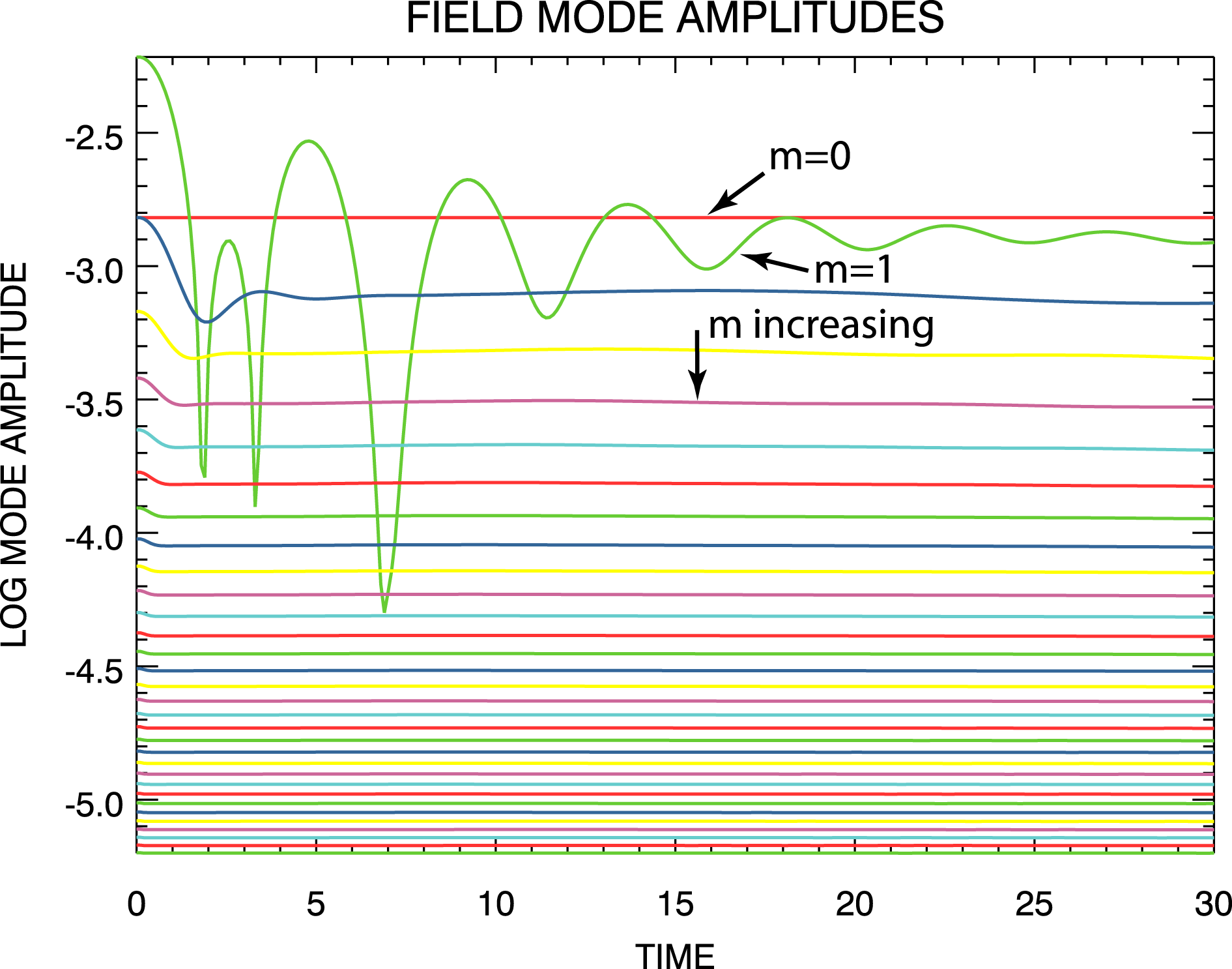
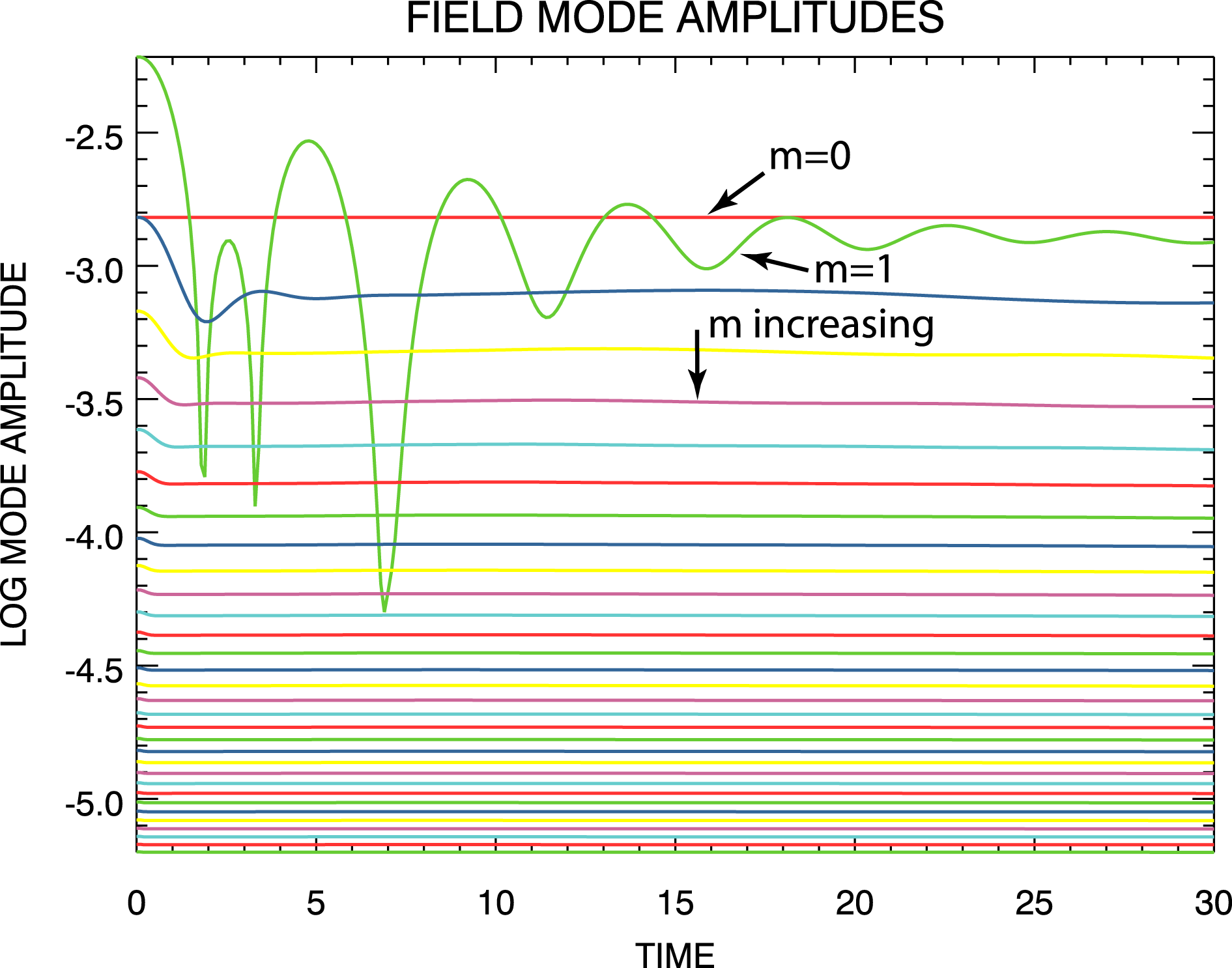
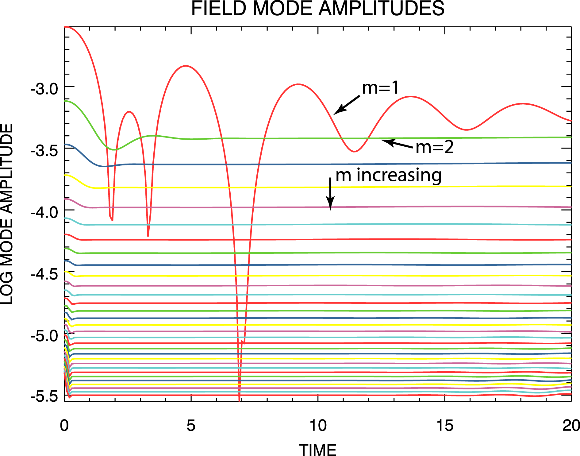
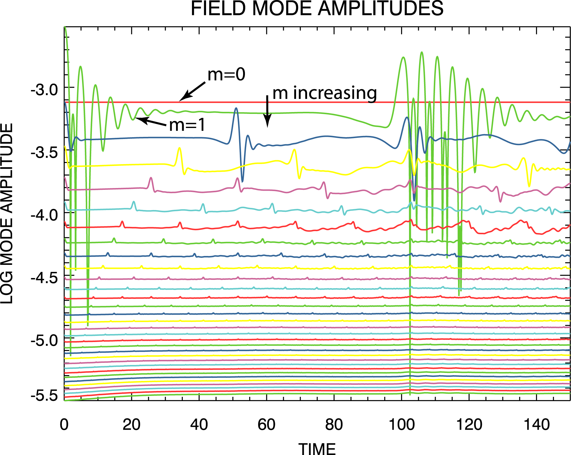
. The evolution with time of the electric field mode magnitudes from the
 $m_{\max }=32$
simulation are shown in figure 1, and the evolution with time of the first 32 electric field mode magnitudes from the
 $m_{\max }=128$
simulation are shown in figure 2.
Electric field mode amplitudes from the
 $m_{\max }=32$
steady density-gradient spectral simulation. The modes are ordered as shown.

Electric field mode amplitudes from the
 $m_{\max }=128$
steady density-gradient spectral simulation. The modes are ordered as shown.

Further, using the same
 $\unicode[STIX]{x1D6FF}f(v,t)=\unicode[STIX]{x1D6FF}f(v,t=0)$
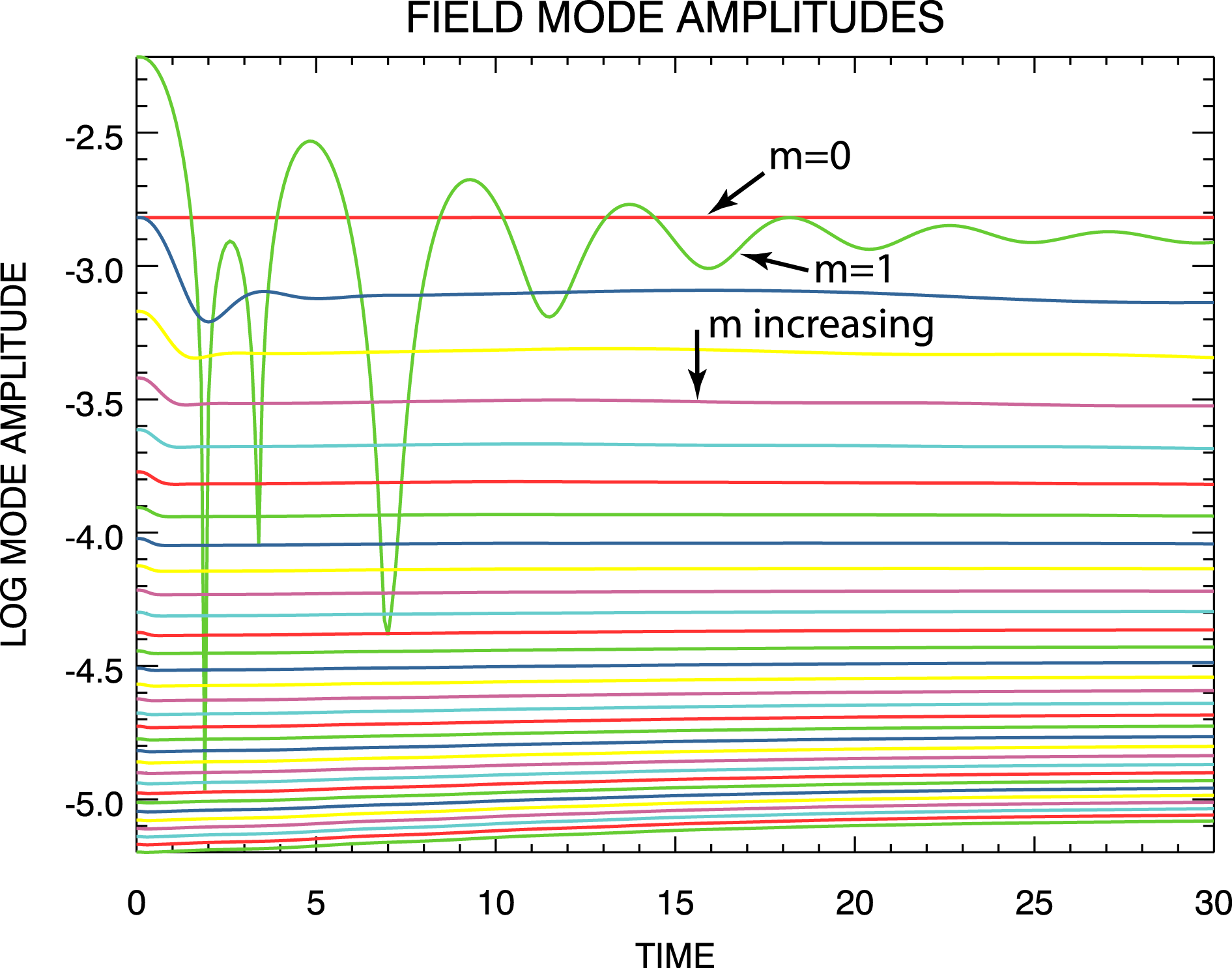
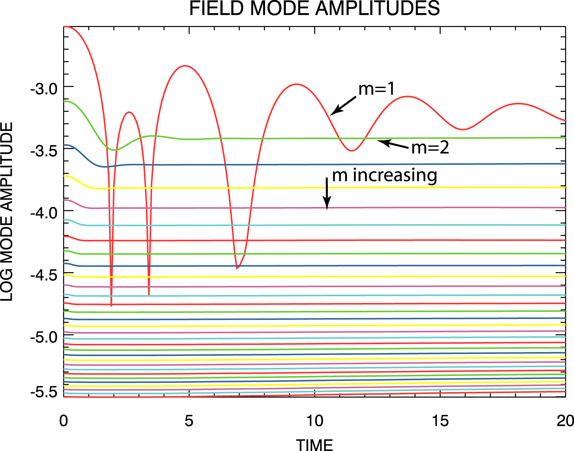
given by (4.3), this non-periodic steady density-gradient solution was also simulated using the flux-balance system. At each time step, the electric field output was Fourier transformed and the field mode magnitudes computed. The evolution with time of the first 32 electric field mode magnitudes from the flux-balance simulation are shown in figure 3.
Electric field mode amplitudes from the steady density-gradient flux-balance simulation. The modes are ordered as shown.

The red curve labelled
 $m=0$
in each of figure 1 thru figure 3 confirms the expected lack of evolution with time of
 $E_{0}(t)$
. The agreement between the
 $m_{\max }=32$
and
 $m_{\max }=128$
spectral simulation results is excellent, indicating that the
 $m_{\max }=32$
simulation contained a sufficient number of spatial Fourier modes. The excellent agreement of the longer wavelength modes for all three simulations provides the first evidence that the spectral system can accurately simulate non-periodic solutions. The slow growth and saturation of the shorter wavelength flux-balance modes disagrees with the spectral results, but we are unable to confirm that this behaviour is real and not a numerical artefact.
4.1.2 Electric field evolution
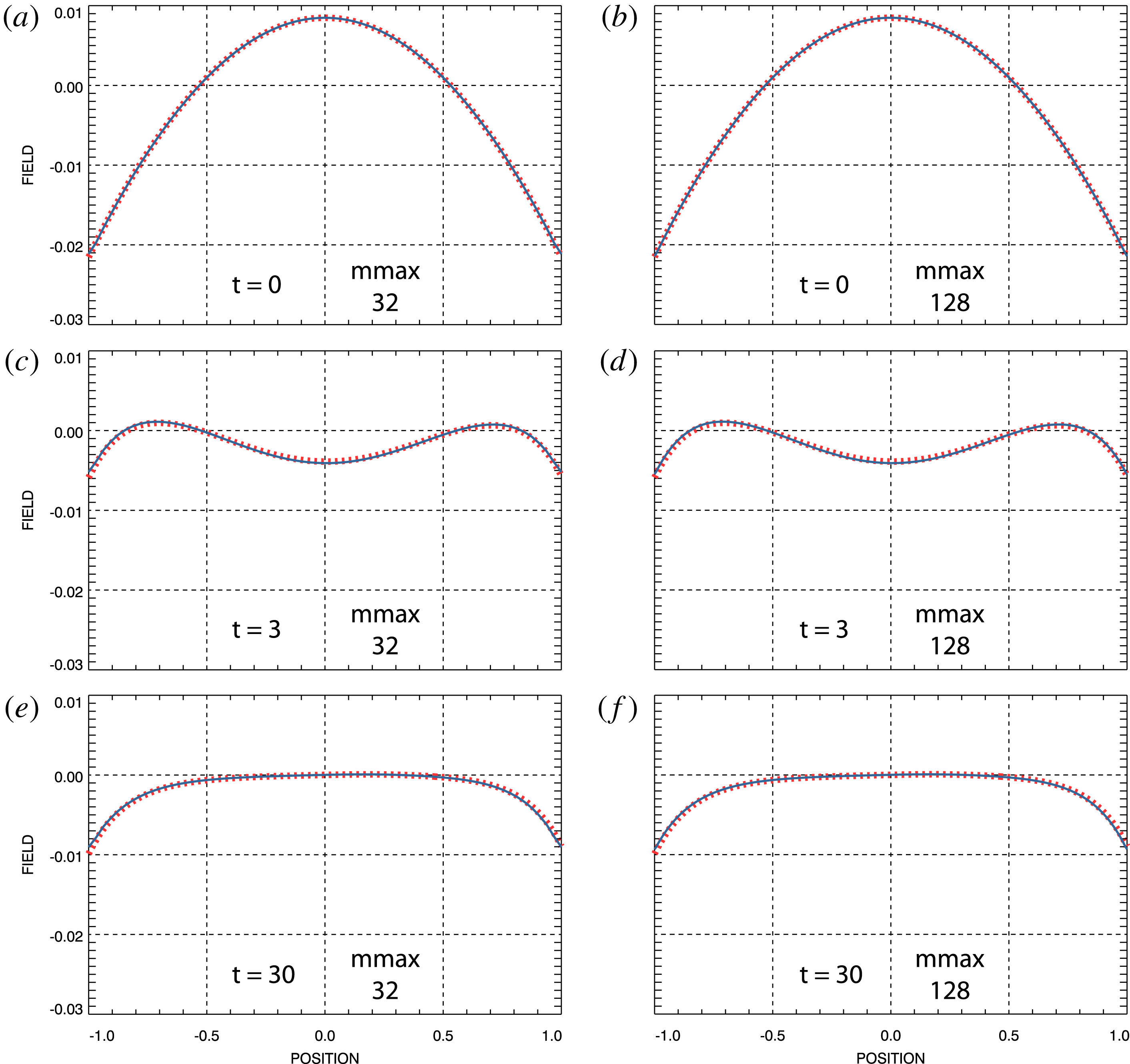
Electric field at selected times. Red, dashed: flux-balance simulation field. Blue: spectral simulation field. (a,c,e) Spectral field from
 $m_{\max }=32$
simulation. (b,d,f) Spectral field from
 $m_{\max }=128$
simulation.

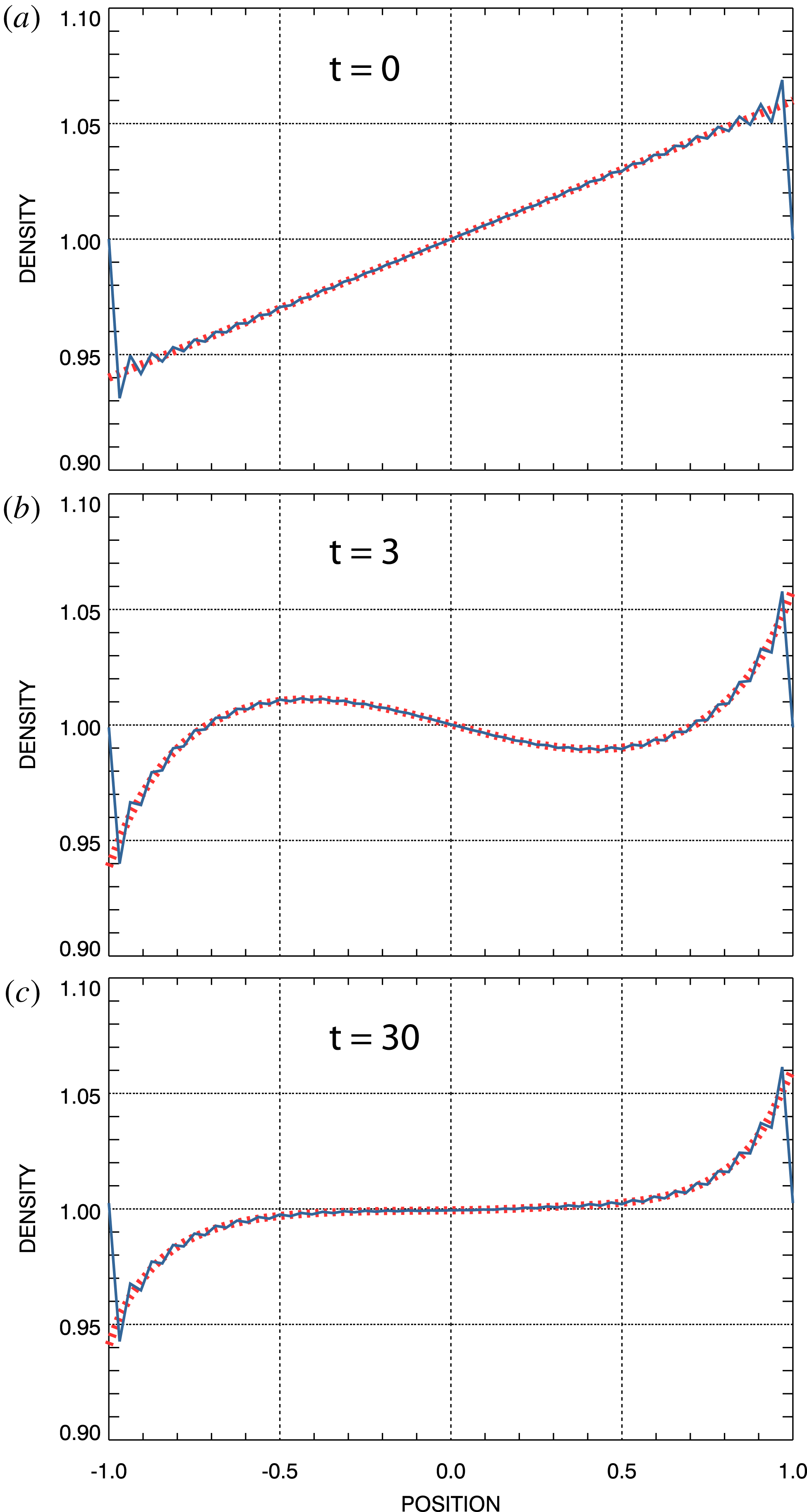
For the overall charge-neutral solutions under consideration here, the electric field remains continuous at the spatial boundaries; i.e. using (2.2)
 $$\begin{eqnarray}\displaystyle \int _{-1}^{1}\text{d}x\frac{\unicode[STIX]{x2202}E}{\unicode[STIX]{x2202}x}=E(1,t)-E(-1,t)=\int _{-1}^{1}\text{d}x[1-n(x,t)]=0. & & \displaystyle\end{eqnarray}$$
However, the non-periodic density-gradient boundary condition ensures that
 $\unicode[STIX]{x2202}E/\unicode[STIX]{x2202}x$
is not continuous at the spatial boundaries. Thus, the electric field is not strictly spatially periodic. Nevertheless, we have found that the field does not exhibit the Gibbs phenomenon.
Figure 4 shows a comparison of the electric fields obtained from the spectral simulations with that obtained from the flux-balance simulation at times
 $t=0$
,
 $t=3$
and at the end of the simulations at
 $t=30$
. This comparison over the entire time interval is shown as movie 1 for the
 $m_{\max }=32$
spectral simulation and as movie 2 for the
 $m_{\max }=128$
spectral simulation available at https://doi.org/10.1017/S0022377819000849. As in figure 4, the red curves in the movies represent the flux-balance simulation fields while the blue curves represent the spectral simulation fields. Overall, the agreement between the flux-balance and the spectral results is excellent, thereby providing further evidence of successful non-periodic solution simulations.
4.1.3 Phase-space distributions
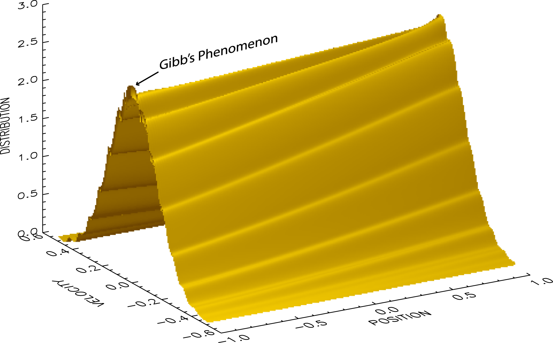
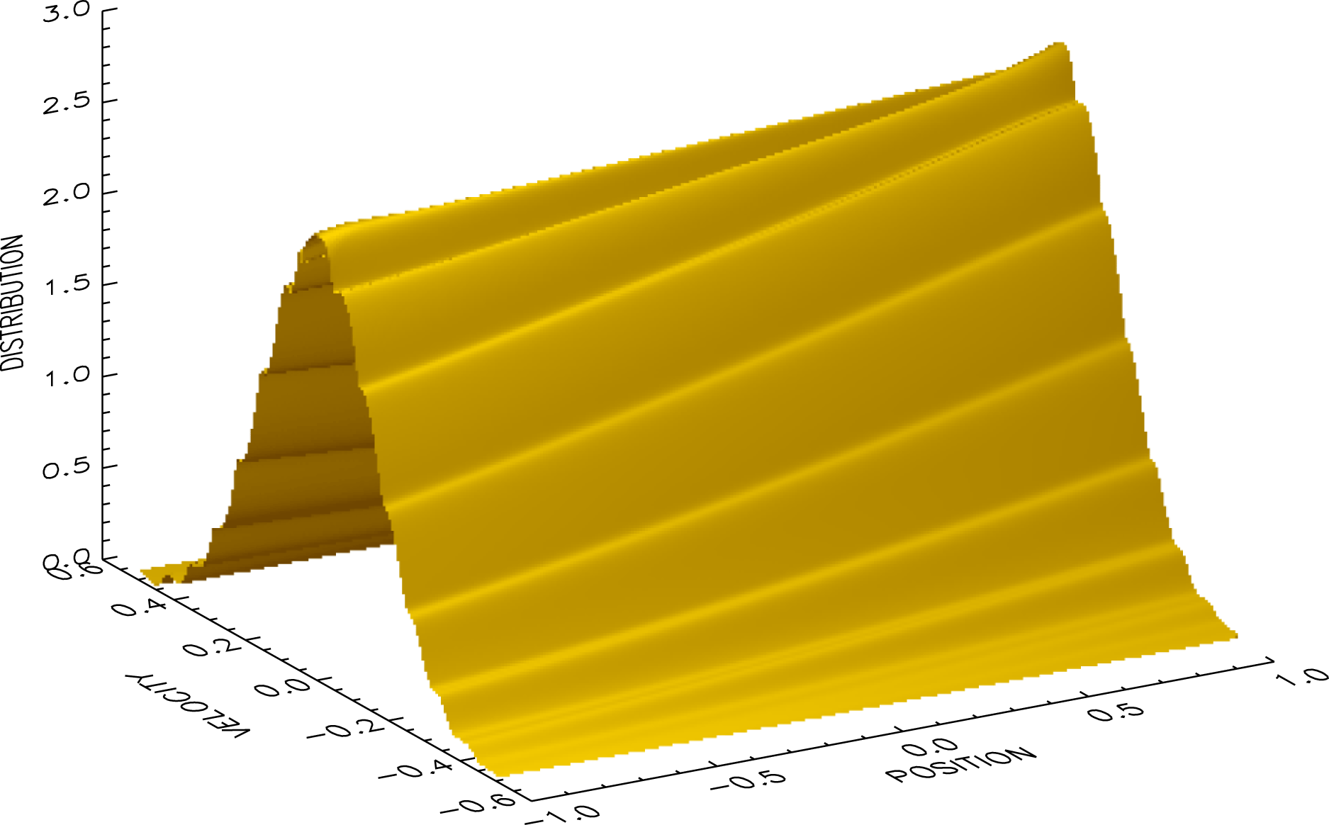
Figure 5 shows the phase-space distribution from the
 $m_{\max }=128$
spectral simulation of the steady density-gradient solution at the end of the simulation
 $t=30$
. For comparison, figure 6 shows the same phase-space distribution from the flux-balance simulation. It can be seen that the two distributions are in good qualitative agreement except for the excesses on the spectral distribution near the spatial boundaries; these are the contributions of the Gibbs phenomenon in the neighbourhoods of the discontinuities of the distribution.
Phase-Space distribution at
 $t=30$
from the
 $m_{\max }=128$
spectral simulation of the steady density-gradient solution.

Phase-space distribution at
 $t=30$
from the flux-balance simulation of the steady density-gradient solution.

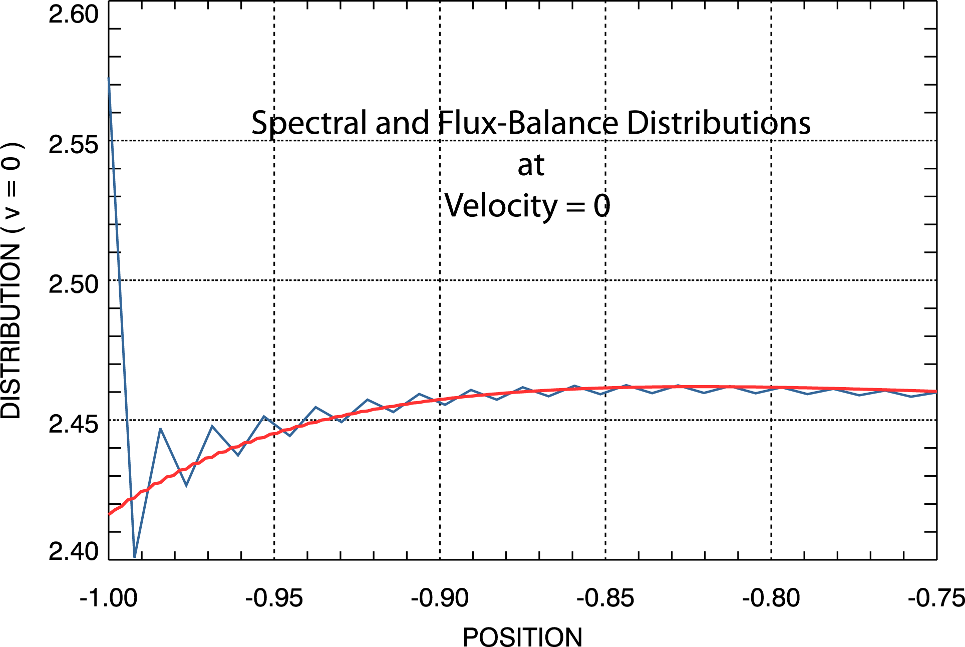
Figure 7 provides a comparison at
 $v=0$
in a small region near
 $x=-1$
of the two distributions shown in figures 5 and 6. The appearance of oscillations due to the Gibbs phenomenon on the spectral distribution is apparent. It is well known that the Gibbs phenomenon arises in truncated Fourier series expansions of discontinuous functions (Gottlieb et al.
Reference Gottlieb, Shu, Solomonoff and Vandeven1992; Jung & Shizgal Reference Jung and Shizgal2004; Gelb & Tanner Reference Gelb and Tanner2006; Adcock, Hansen & Shadrin Reference Adcock, Hansen and Shadrin2014). The Gibbs phenomenon appears in the transformation from the Fourier space to the position space; i.e. it is the truncated inverse Fourier transformation process that produces the Gibbs phenomenon. The Gibbs oscillations do not exist in the transformed space, only in the position space. The spectral system operates entirely in the Fourier transformed space where the Gibbs phenomenon does not exist. It is impossible for the Gibbs phenomenon to affect the evolution of the spectral system in that space. Further, we provide preliminary results below in § 5 that demonstrate how these oscillations may be removed in post-processing of the spectral simulation results.


4.1.4 Density evolution
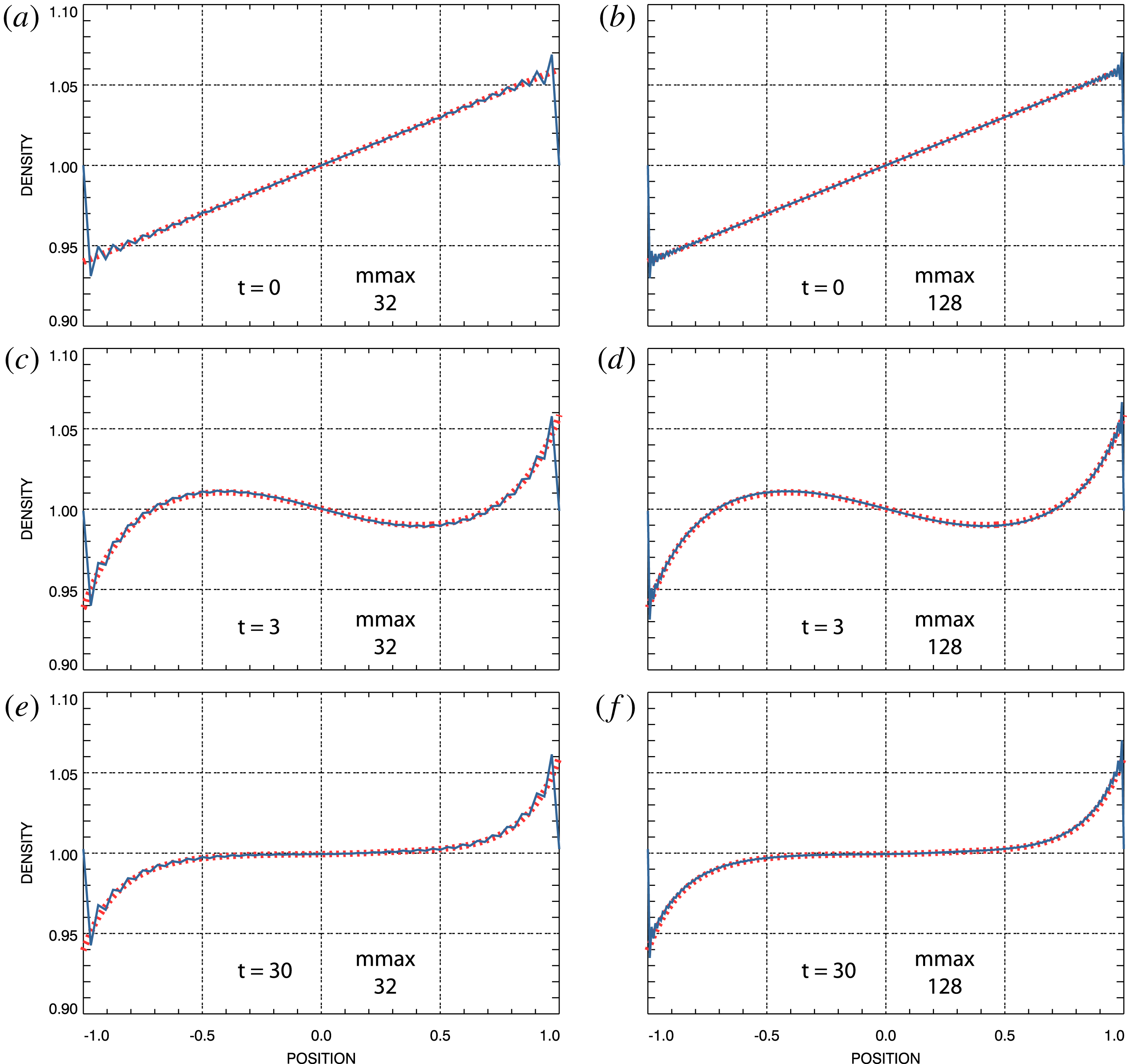
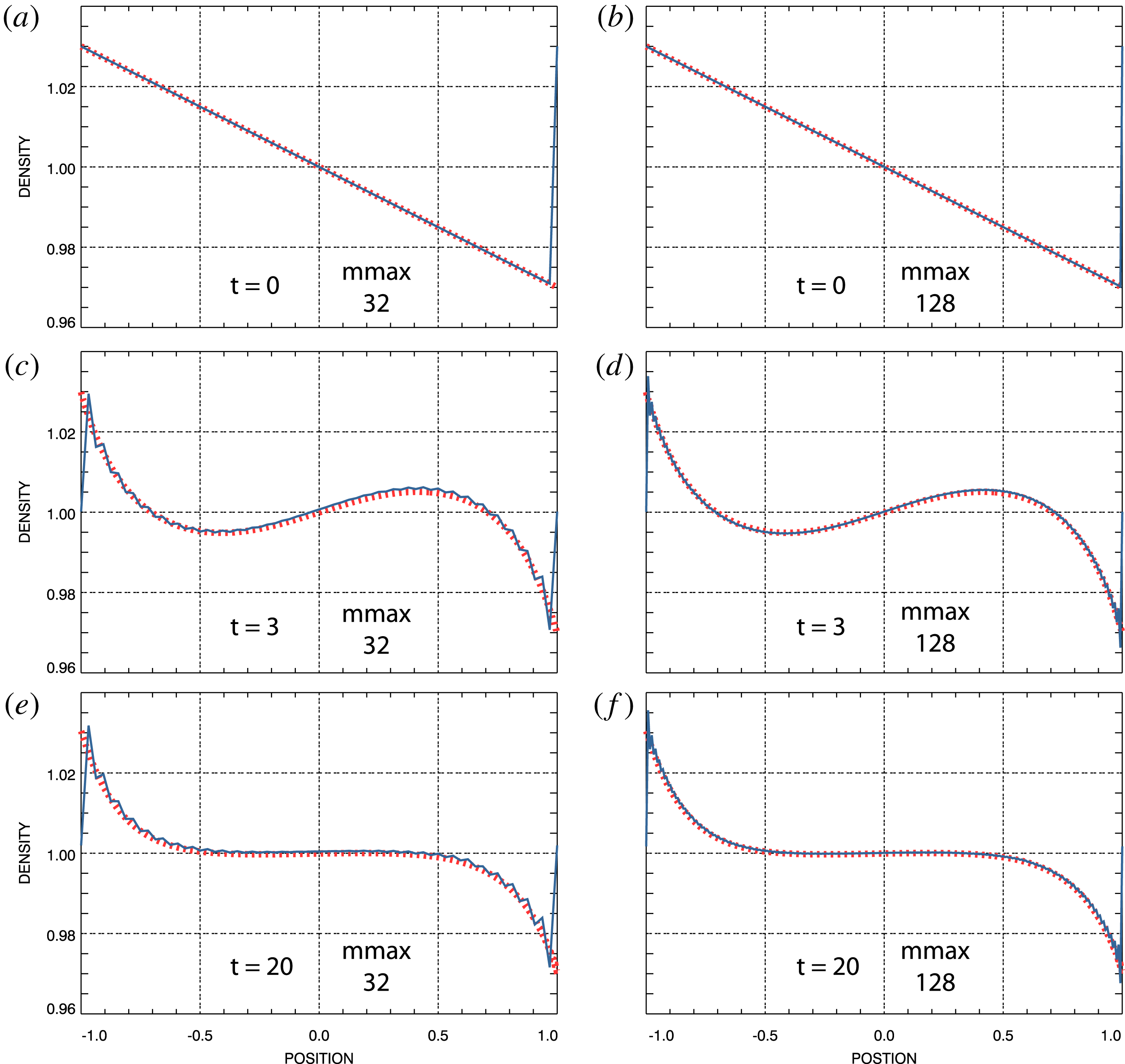
A more quantitative indication of the agreement of the spectral simulation phase-space distributions with that of the flux-balance simulation is provided by figure 8. Electron densities at selected times from both spectral simulations plus the flux-balance simulation of the steady density-gradient solution are shown. The densities shown have been constructed by numerically integrating the respective simulated phase-space distributions over velocity; disparities in the distributions could be expected to lead to disparities in the densities. Particularly in the case of the
 $m_{\max }=32$
spectral simulation, the appearance of oscillations due to the Gibbs phenomenon near the boundaries at
 $x=\pm 1$
is clear. The oscillations on the
 $m_{\max }=128$
densities are not reduced in magnitude compared to those on the
 $m_{\max }=32$
densities but they reside in more compressed regions near the boundaries, thus making their appearance on the figure less apparent.
Electron density at selected times. Red, dashed: flux-balance simulation. Blue: spectral simulation. (a,c,e) Spectral density from
 $m_{\max }=32$
simulation. (b,d,f) Spectral density from
 $m_{\max }=128$
simulation.

As explained above (4.1)–(4.3), these simulations have been initialized with thermal distributions containing a linear spatial perturbation such that their densities exhibit the linear spatial dependence shown in figure 8(a,b), with spatial average 1. The difference
 $\unicode[STIX]{x1D6FF}f(v,t)=\unicode[STIX]{x1D6FF}f(v,t=0)$
has been maintained then for the remainder of the simulations. It is important to note that the values
 $f(\pm 1,v,t)$
have not been controlled and are free to evolve. As time increases, the densities evolve to the final state shown in figure 8(e,f) with several interim overshoots, such as in (c,d) at
 $t=3$
. Further details of the evolution captured in figure 8(a,c,e)
 $(m_{\max }=32)$
and figure 8(b,d,f)
 $(m_{\max }=128)$
are contained in movie 3 and movie 4, respectively.
Overall, it appears that the spectral densities and the flux-balance density are in excellent agreement, except for the appearance of the oscillations due to the Gibbs phenomenon on the spectral results. Again, these results support the conclusion that for this simple example
 $m_{\max }=32$
is sufficient. Clearly, other examples may require more Fourier modes. Even so, the evidence that we have presented here suggests more generally that non-periodic solutions can be simulated using the doubly Fourier transformed spectral system. The removal of the Gibbs phenomenon from the spectral results will be discussed below in § 5.
4.1.5 Conservation
For the steady density-gradient solution
 $\unicode[STIX]{x1D6FF}f(v)$
, given by (4.1) and (4.3), is an even function of the velocity
 $v$
. Therefore,
 $u(1,t)-u(-1,t)=0$
, as it must be to conserve charge neutrality, and from (3.17) the space-averaged electron density is expected to remain constant at its original value,
 $n_{0}(t)=1$
.
Because
 $\unicode[STIX]{x1D6FF}f(v)$
is constant in time for this solution,
 $\unicode[STIX]{x1D6FF}\overline{P}-v_{f}^{2}\unicode[STIX]{x1D6FF}n$
does not evolve with time as well. The initial electron distribution, equations (4.1) and (4.2), does not support an electron flux; i.e.
 $u_{0}(t=0)=0$
in (2.9). The initial space-averaged electric field has been set to
 $E_{0}(t=0)=-1/2(\unicode[STIX]{x1D6FF}\overline{P}-v_{f}^{2}\unicode[STIX]{x1D6FF}n)$
and therefore, from (2.9)
 $E_{0}(t)=E_{0}(t=0)$
and we expect
 $u_{0}(t)=u_{0}(t=0)=0$
for the space-averaged electron flux.
Because
 $\unicode[STIX]{x1D6FF}f(v)$
is an even function of the velocity
 $v$
,
 $u(1,t)-u(-1,t)=0$
and
 $\overline{\unicode[STIX]{x1D6E4}}(1,t)-\overline{\unicode[STIX]{x1D6E4}}(-1,t)=0$
in (3.20). Thus, from (3.20) we expect the space-averaged, filtered total energy
 $$\begin{eqnarray}\displaystyle \overline{P}_{0}(t)+\frac{1}{2}\int _{-1}^{1}\text{d}x\,E^{2}(x,t) & & \displaystyle\end{eqnarray}$$
to be a conserved quantity in the steady density-gradient solution.
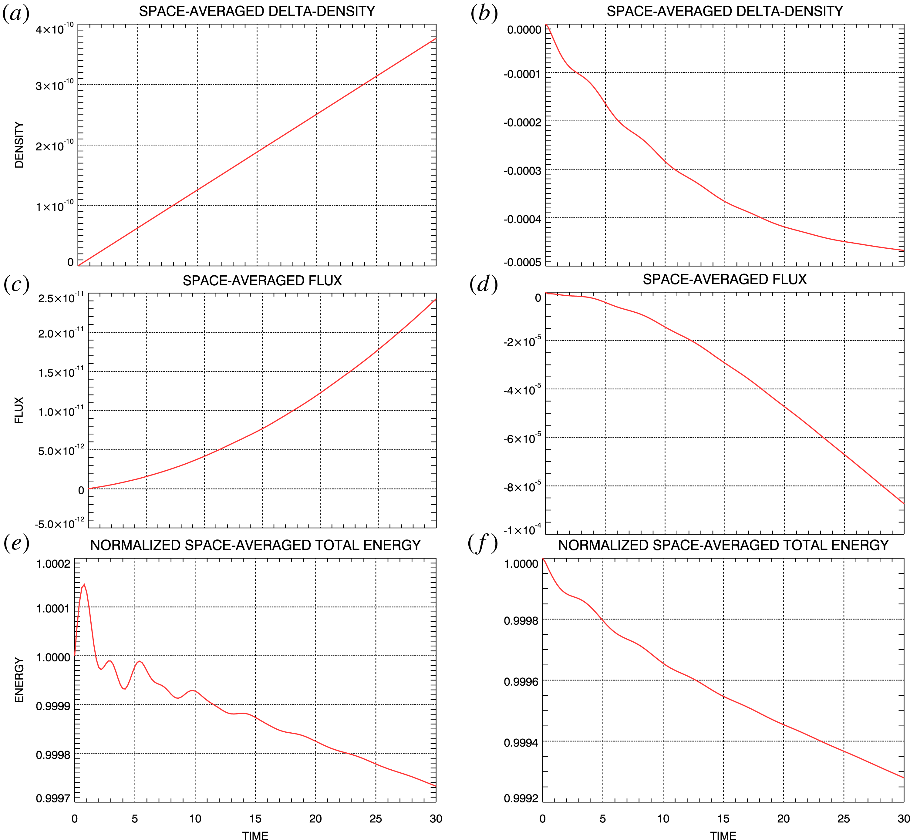
Conserved quantities for steady density-gradient simulations. (a,c,e) Spectral simulation. (b,d,f) Flux-balance simulation. (a,b) Space-averaged density change. (c,d) Space-averaged electron flux. (e,f) Filtered total energy.

Figure 9 shows the evolution with time of the space-averaged density, flux, and filtered total energy obtained from the steady density-gradient simulations. Panel (a,c,e) shows results from the spectral simulation using
 $m_{\max }=128$
and those in (b,d,f) show results from the flux-balance simulation. Panel (a,b) shows the change in space-averaged density relative to its initial value
 $n_{0}(t=0)=1$
. Panel (c,d) shows the space-averaged electron flux evolution from the spectral and flux-balance simulations and panel (e,f) shows the space-averaged total filtered energy evolution. Changes in all of these quantities are quite small over the course of the respective simulations. The spectral results are generally better than the flux-balance results but satisfactory accuracy in both of the simulations is indicated.
4.2 Steady density and temperature gradients
For our second non-periodic simulation example we consider an electron plasma whose initial state is the spatially dependent thermal distribution
 $$\begin{eqnarray}\displaystyle f(x,v,t=0)=\left(1+\frac{\unicode[STIX]{x1D6FC}}{2}x\right)\frac{1}{v_{\text{th}}(x)\sqrt{2\unicode[STIX]{x03C0}}}\exp \left(-\frac{1}{2}\left(\frac{v}{v_{\text{th}}(x)}\right)^{2}\right), & & \displaystyle\end{eqnarray}$$
with
 $$\begin{eqnarray}\displaystyle v_{\text{th}}(x)=v_{\text{th}0}\sqrt{1+\frac{\unicode[STIX]{x1D6FD}}{2}x}, & & \displaystyle\end{eqnarray}$$
in which
 $\unicode[STIX]{x1D6FD}$
is a free parameter that controls the strength of the temperature gradient and, following Cheng & Knorr (Reference Cheng and Knorr1976),
 $v_{\text{th}0}=0.5/\unicode[STIX]{x03C0}$
. In this case
 $$\begin{eqnarray}\displaystyle & & \displaystyle \unicode[STIX]{x1D6FF}f(v,t=0)=f(1,v,t=0)-f(-1,v,t=0)\nonumber\\ \displaystyle & & \displaystyle \quad =\frac{(1+\unicode[STIX]{x1D6FC}/2)}{v_{\text{th}0}\sqrt{2\unicode[STIX]{x03C0}(1+\unicode[STIX]{x1D6FD}/2)}}\exp \left(-\frac{1}{2(1+\unicode[STIX]{x1D6FD}/2)}\left(\frac{v}{v_{\text{th}0}}\right)^{2}\right)\nonumber\\ \displaystyle & & \displaystyle \qquad -\,\frac{(1-\unicode[STIX]{x1D6FC}/2)}{v_{\text{th}0}\sqrt{2\unicode[STIX]{x03C0}(1-\unicode[STIX]{x1D6FD}/2)}}\exp \left(-\frac{1}{2(1-\unicode[STIX]{x1D6FD}/2)}\left(\frac{v}{v_{\text{th}0}}\right)^{2}\right),\end{eqnarray}$$
which is compatible with the condition (3.13) for maintaining a charge-neutral plasma and, again, we set
 $\unicode[STIX]{x1D6FF}f(v,t)=\unicode[STIX]{x1D6FF}f(v,t=0)$
. For this distribution, the pressure difference across the spatial domain is given by
 $$\begin{eqnarray}\displaystyle \unicode[STIX]{x1D6FF}P=\int _{-\infty }^{\infty }\text{d}v\,v^{2}\unicode[STIX]{x1D6FF}f(v,t=0)=v_{\text{th}0}^{2}(\unicode[STIX]{x1D6FD}+\unicode[STIX]{x1D6FC}). & & \displaystyle\end{eqnarray}$$
We choose
 $\unicode[STIX]{x1D6FC}=-\unicode[STIX]{x1D6FD}=-0.03$
to obtain
 $\unicode[STIX]{x1D6FF}P=0$
and therefore, from (2.9), with
 $E_{0}(t=0)=1/2v_{f}^{2}\unicode[STIX]{x1D6FF}n$
and
 $u_{0}(t=0)=0$
we have
 $E_{0}(t)=E_{0}(t=0)$
. This ‘steady density-temperature-gradient solution’ remains in overall pressure equilibrium for
 $t\geqslant 0$
using density and temperature gradients in opposing directions.
4.2.1 Electric field mode amplitudes
Electric field mode amplitudes from the
 $m_{\max }=32$
steady density-temperature-gradient spectral simulation. The modes are ordered as shown.

Two spectral system simulations of the steady density-temperature-gradient solution have been carried out. For the first,
 $m_{\max }=32$
and for the second
 $m_{\max }=128$
. The evolution with time of the electric field mode magnitudes from the
 $m_{\max }=32$
simulation is shown in figure 10. As for the steady density-gradient simulations discussed in the preceding section, the field mode magnitudes of the
 $m_{\max }=32$
and
 $m_{\max }=128$
simulations have been found effectively identical. Consequently, the
 $m_{\max }=128$
field mode magnitudes are not displayed. We conclude that the
 $m_{\max }=32$
simulation contained a sufficient number of spatial Fourier modes for an accurate approximation to the steady density-temperature-gradient solution. With the same
 $\unicode[STIX]{x1D6FF}f(v,t)=\unicode[STIX]{x1D6FF}f(v,t=0)$
given by (4.10), this non-periodic solution was also simulated using the flux-balance system. Figures 10 and 11 provide a comparison of the field mode amplitude evolution obtained from the spectral simulation with
 $m_{\max }=32$
and the flux-balance simulation of the steady density-temperature-gradient solution. The comparison indicates excellent agreement between the two simulations.
Electric field mode amplitudes from the steady density-temperature-gradient flux-balance simulation. The modes are ordered as shown.

4.2.2 Electric field evolution
Electric field at selected times. Red, dashed: flux-balance simulation field. Blue: spectral simulation field. (a,c,e) Spectral field from
 $m_{\max }=32$
simulation. (b,d,f) Spectral field from
 $m_{\max }=128$
simulation.

For this steady density-temperature-gradient solution, figure 12 shows a comparison of the electric fields obtained from the spectral simulations with that obtained from the flux-balance simulation at times
 $t=0$
,
 $t=3$
, and at the end of the simulations at
 $t=20$
. This comparison over the entire time interval is shown as movie 5 for the
 $m_{\max }=32$
spectral simulation and as movie 6 for the
 $m_{\max }=128$
spectral simulation. As in figure 12, the red curves in the movies represent the flux-balance simulation fields while the blue curves represent the spectral simulation fields. Overall, the agreement between the flux-balance and the spectral results is excellent, thereby providing further evidence of successful non-periodic solution simulations.
4.2.3 Density and temperature evolution
Electron density at selected times. Red, dashed: flux-balance simulation. Blue: spectral simulation. (a,c,e) Spectral density from
 $m_{\max }=32$
simulation. (b,d,f) Spectral density from
 $m_{\max }=128$
simulation.

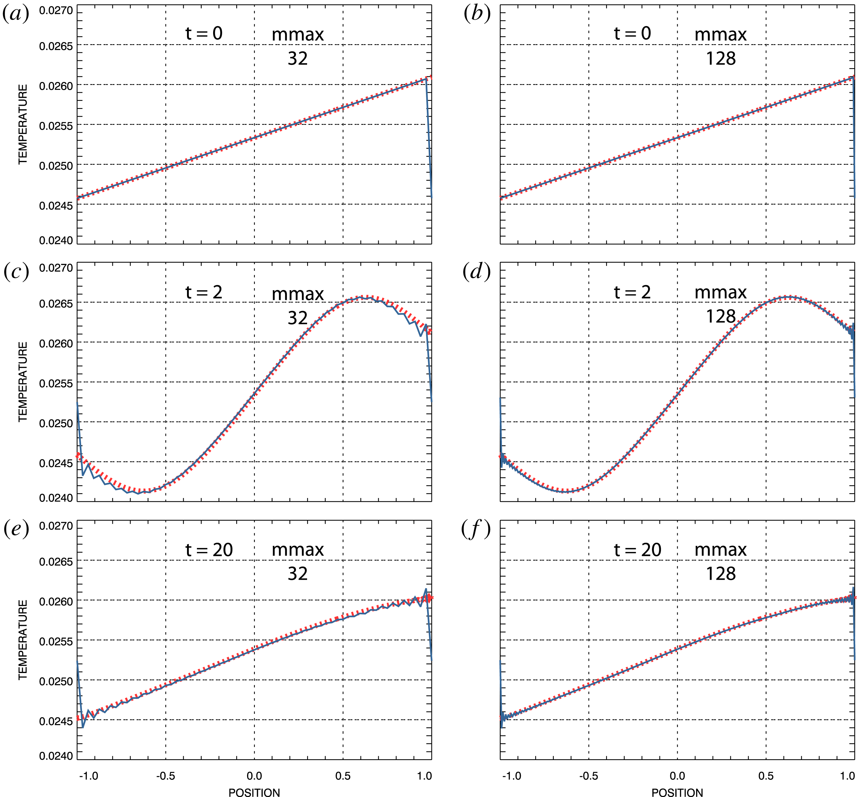
The density and temperature obtained from the spectral and flux-balance steady density-temperature-gradient simulations are displayed at selected times in figures 13 and 14 respectively. Results from the
 $m_{\max }=32$
spectral simulation are shown in the left columns and results from the
 $m_{\max }=128$
simulation are shown on the right. The flux-balance results are shown as red dashed curves throughout. The results shown have been constructed by numerically integrating the respective simulated phase-space distributions over velocity; disparities in the distributions could be expected to lead to disparities in the densities and/or temperatures.
Both the density and temperature generally exhibit oscillations due to the Gibbs phenomenon near the spatial boundaries, with the exception at
 $t=0$
. In contrast to the density-gradient simulations discussed in the preceding section, an analytic expression for a Fourier series expansion of the initial distribution (4.8) and (4.9) is not available. Consequently, at
 $t=0$
the data for initializing the spectral simulations were created by numerically Fourier transforming the initial distribution (4.8) and (4.9). Before marching on, the spectral data were inverse Fourier transformed to output the computed initial distribution. The result was, of course, identical to the inputted initial distribution to within numerical precision, with no Gibbs phenomenon superposed. The oscillations due to the Gibbs phenomenon appeared on the phase-space distribution and its moments in just a few time steps later in the simulations.
Electron temperature at selected times. Red, dashed: flux-balance simulation. Blue: spectral simulation. (a,c,e) Spectral temperature from
 $m_{\max }=32$
simulation. (b,d,f) Spectral temperature from
 $m_{\max }=128$
simulation.

It can be seen that the density and temperature distributions were initialized containing linear spatial gradients in opposing directions. These were adjusted in strength and sense according to (4.11) with
 $\unicode[STIX]{x1D6FC}=-\unicode[STIX]{x1D6FD}$
so that the simulated plasma was initialized and remained
 $(\unicode[STIX]{x1D6FF}f(v,t)=\unicode[STIX]{x1D6FF}f(v,t=0))$
in overall pressure balance. Even so, the phase-space distribution and its moments evolved considerably as they relaxed to the final state shown, for the moments, in figures 13(e,f) and 14(e,f) and, for the electric field, in figure 12(e,f). In the end, the temperature distribution is modified only slightly from its initial state. The final density distribution can be reasonably well fit by the expression
 $1.0+\unicode[STIX]{x1D6FC}x^{5}$
.
Further details of the density evolution captured in figure 13(a,c,e)
 $(m_{\max }=32)$
and figure 13(b,d,f)
 $(m_{\max }=128)$
are contained in movie 7 and movie 8, respectively. In addition, further details of the temperature evolution captured in figure 14(a,c,e)
 $(m_{\max }=32)$
and figure 14(b,d,f)
 $(m_{\max }=128)$
are contained in movie 9 and movie 10, respectively. The red curves in the movies represent the flux-balance simulation results while the blue curves represent the spectral simulation results. As noted above, the difference
 $\unicode[STIX]{x1D6FF}f(v,t)=\unicode[STIX]{x1D6FF}f(v,t=0)$
has been maintained over the course of these simulations but the values
 $f(\pm 1,v,t)$
are free to evolve. Movie 9 and Movie 10 provide an example of this freedom; the temperatures at the boundaries can be seen to evolve noticeably near the ends of the movies.
Except for the appearance of the Gibbs phenomenon, the spectral and flux-balance simulation results for the steady density-temperature-gradient solution are in excellent agreement.
4.2.4 Conservation
For the steady density-temperature-gradient solution
 $\unicode[STIX]{x1D6FF}f(v)$
, given by (4.10), is an even function of the velocity
 $v$
. Therefore,
 $u(1,t)-u(-1,t)=0$
, as it must be to conserve charge neutrality, and from (3.17) the space-averaged electron density is expected to remain constant at its original value,
 $n_{0}(t)=1$
.
Because
 $\unicode[STIX]{x1D6FF}f(v)$
is constant in time for this solution,
 $\unicode[STIX]{x1D6FF}\overline{P}-v_{f}^{2}\unicode[STIX]{x1D6FF}n$
does not evolve with time as well. The initial electron distribution, equations (4.8) and (4.9), does not support an electron flux; i.e.
 $u_{0}(t=0)=0$
in (2.9). We have chosen
 $\unicode[STIX]{x1D6FC}=-\unicode[STIX]{x1D6FD}=-0.03$
in (4.11) to obtain
 $\unicode[STIX]{x1D6FF}P=0$
. The initial space-averaged electric field has been set to
 $E_{0}(t=0)=1/2v_{f}^{2}\unicode[STIX]{x1D6FF}n$
and therefore, from (2.9)
 $E_{0}(t)=E_{0}(t=0)$
and we expect
 $u_{0}(t)=u_{0}(t=0)=0$
for the space-averaged electron flux.
Because
 $\unicode[STIX]{x1D6FF}f(v)$
is an even function of the velocity
 $v$
,
 $u(1,t)-u(-1,t)=0$
and
 $\overline{\unicode[STIX]{x1D6E4}}(1,t)-\overline{\unicode[STIX]{x1D6E4}}(-1,t)=0$
in (3.20). Thus, from (3.20) we expect the space-averaged, filtered total energy
 $$\begin{eqnarray}\displaystyle \overline{P}_{0}(t)+\frac{1}{2}\int _{-1}^{1}\text{d}x\,E^{2}(x,t) & & \displaystyle\end{eqnarray}$$
to be a conserved quantity in the steady density-temperature-gradient solution.
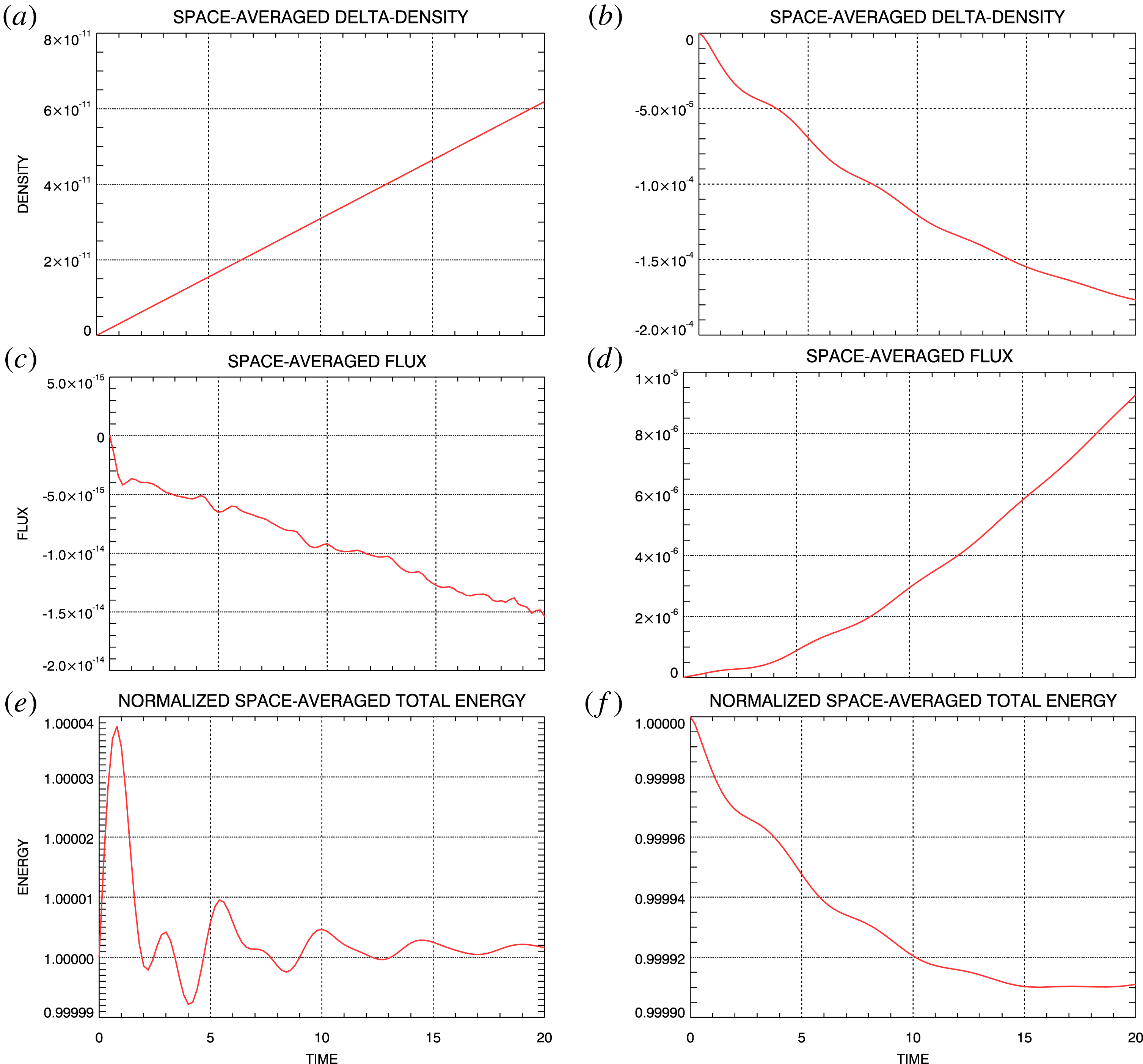
Conserved quantities for steady density-temperature-gradient simulations. (a,c,e) Spectral simulation. (b,d,e) Flux-balance simulation. (a,b) Space-averaged density change. (c,d) Space-averaged electron flux. (e,f) Filtered total energy.

Figure 15 shows the evolution with time of the space-averaged density, flux and filtered total energy obtained from the steady density-temperature-gradient simulations. Panel (a,c,e) shows results from the spectral simulation using
 $m_{\max }=128$
and those in (b,d,f) show results from the flux-balance simulation. Panel (a,b) shows the change in space-averaged density relative to its initial value
 $n_{0}(t=0)=1$
. Panel (c,d) shows the space-averaged electron flux evolution from the spectral and flux-balance simulations and panel (e,f) shows the space-averaged total filtered energy evolution. Changes in all of these quantities are quite small over the course of the respective simulations. The spectral results are generally better than the flux-balance results but satisfactory accuracy in both of the simulations is indicated.
5 Inverse polynomial reconstruction method
Following the seminal work of Gottlieb et al. (Reference Gottlieb, Shu, Solomonoff and Vandeven1992) and Gottlieb & Shu (Reference Gottlieb and Shu1997), a large body of research has been developed concerning the properties of the Gibbs phenomenon and its removal from truncated Fourier series expansions of discontinuous functions. Out of this, we have chosen to apply the inverse polynomial reconstruction method due to Shizgal & Jung (Reference Shizgal and Jung2003) and Jung & Shizgal (Reference Jung and Shizgal2004, Reference Jung and Shizgal2005, Reference Jung and Shizgal2007) to remove the Gibbs phenomenon from the non-periodic spectral simulation results. We have settled on the IPRM due to its relative stability and accuracy and because it has been extended to two-dimensional functions (Jung & Shizgal Reference Jung and Shizgal2005; Abdi & Hosseini Reference Abdi and Hosseini2008), thereby making it possible to look forward to applying the method to the phase-space distribution. In the following, however, we limit our discussion to an application to the one-dimensional density from the steady density-gradient simulation to provide a demonstration of the effectiveness of the IPRM.
5.1 Implementation
Jung & Shizgal (Reference Jung and Shizgal2004) provide a complete description of the implementation of the IPRM in one dimension. In this section, we give a summary of the restricted version of their implementation that we have carried out.
We begin with a truncated Fourier series expansion
 $$\begin{eqnarray}\displaystyle \unicode[STIX]{x1D70C}_{N}(x)=\mathop{\sum }_{k=-N}^{N}\unicode[STIX]{x1D70C}_{k}\exp (\text{i}\unicode[STIX]{x03C0}kx), & & \displaystyle\end{eqnarray}$$
in which the
 $\unicode[STIX]{x1D70C}_{k}$
are the Fourier coefficients
 $$\begin{eqnarray}\displaystyle \unicode[STIX]{x1D70C}_{k}=\frac{1}{2}\int _{-1}^{1}\unicode[STIX]{x1D70C}(x)\exp (-\text{i}\unicode[STIX]{x03C0}kx)\,\text{d}x & & \displaystyle\end{eqnarray}$$
of the density
 $\unicode[STIX]{x1D70C}(x)$
on the interval
 $x\in (-1,1)$
. Our goal is to extract
 $\unicode[STIX]{x1D70C}(x)$
from the truncated expansion (5.1), written as a finite sum of Legendre polynomials
 $$\begin{eqnarray}\displaystyle \unicode[STIX]{x1D70C}_{m}(x)=\mathop{\sum }_{l=0}^{m}g_{l}P_{l}(x). & & \displaystyle\end{eqnarray}$$
(The IPRM due to Jung and Shizdal yields a more general finite sum of Gegenbauer polynomials
 $C_{l}^{\unicode[STIX]{x1D706}}(x)$
. We have chosen the special case,
 $C_{l}^{\unicode[STIX]{x1D706}=1/2}(x)=P_{l}(x)$
.) The accuracy with which
 $\unicode[STIX]{x1D70C}_{m}(x)$
represents
 $\unicode[STIX]{x1D70C}(x)$
is a central issue in the work of Jung and Shizdal.
In our application to the spectral system simulation results, the
 $\unicode[STIX]{x1D70C}_{k}$
are obtained directly from the raw simulation output. From (3.1)
 $$\begin{eqnarray}\displaystyle \overline{K}_{k}(\unicode[STIX]{x1D707}=0,t)=\frac{1}{2}\int _{-1}^{1}\text{d}x\,\text{e}^{-\text{i}k\unicode[STIX]{x03C0}x}\int _{-\infty }^{\infty }\text{d}v\,\overline{f}(x,v,t)=\frac{1}{2}\int _{-1}^{1}\text{d}x\,\text{e}^{-\text{i}k\unicode[STIX]{x03C0}x}\unicode[STIX]{x1D70C}(x,t)=\unicode[STIX]{x1D70C}_{k}, & & \displaystyle\end{eqnarray}$$
and
 $\unicode[STIX]{x1D70C}_{N}(x)$
from (5.1) is the density, e.g. shown in figure 8, containing the Gibbs phenomenon.
A transformation matrix
 $\unicode[STIX]{x1D652}$
can be defined through
 $$\begin{eqnarray}\displaystyle W_{k,l}=\frac{1}{2}\int _{-1}^{1}P_{l}(x)\exp (-\text{i}k\unicode[STIX]{x03C0}x)\,\text{d}x. & & \displaystyle\end{eqnarray}$$
Jung and Shizdal have shown that the expansion coefficients
 $g_{l}$
in (5.3) can be obtained through the solution of the equation
 $$\begin{eqnarray}\displaystyle \mathop{\sum }_{l=0}^{m}W_{k,l}g_{l}=\unicode[STIX]{x1D70C}_{k}, & & \displaystyle\end{eqnarray}$$
with
 $m=2N$
so that
 $\unicode[STIX]{x1D652}$
is a square matrix of dimension
 $(2N+1)\times (2N+1)$
.
5.1.1 Method 1
The most straight forward approach to a solution of (5.6) is to invert the square matrix
 $\unicode[STIX]{x1D652}$
; i.e.
 $$\begin{eqnarray}\displaystyle g_{l}=\mathop{\sum }_{k=-N}^{N}(\unicode[STIX]{x1D652}^{-1})_{l,k}\unicode[STIX]{x1D70C}_{k}. & & \displaystyle\end{eqnarray}$$
However, Jung and Shizdal do not recommend this method for reasons of numerical accuracy and speed. They suggest a second method that takes advantage of some symmetry properties of
 $\unicode[STIX]{x1D652}$
and the
 $g_{l}$
plus the reality properties of the Fourier coefficients
 $\unicode[STIX]{x1D70C}_{k}$
.
5.1.2 Method 2
Following Jung and Shizdal, we introduce two new matrices
 $$\begin{eqnarray}\displaystyle \left.\begin{array}{@{}c@{}}\displaystyle \unicode[STIX]{x1D64F}=\text{Im}\unicode[STIX]{x1D652}\quad \unicode[STIX]{x1D651}=\text{Re}\unicode[STIX]{x1D652}\\ \displaystyle \unicode[STIX]{x1D652}=\unicode[STIX]{x1D651}+\text{i}\unicode[STIX]{x1D64F}.\end{array}\right\} & & \displaystyle\end{eqnarray}$$
Then
 $$\begin{eqnarray}\displaystyle \left.\begin{array}{@{}c@{}}\displaystyle T_{k,l}=-\frac{1}{2}\int _{-1}^{1}P_{l}(x)\sin k\unicode[STIX]{x03C0}x\,\text{d}x\quad l\text{ odd}\\ \displaystyle V_{k,l}=\frac{1}{2}\int _{-1}^{1}P_{l}(x)\cos k\unicode[STIX]{x03C0}x\,\text{d}x\quad l\text{ even}\end{array}\right\} & & \displaystyle\end{eqnarray}$$
and
 $$\begin{eqnarray}\displaystyle \left.\begin{array}{@{}c@{}}T_{k,l}=0\quad l\text{ even},\text{ all }k\\ V_{k,l}=0\quad l\text{ odd},\text{ all }k.\end{array}\right\} & & \displaystyle\end{eqnarray}$$
From (5.3), the
 $g_{l}$
must be real. Thus, taking the real and imaginary parts of (5.6) leads to
 $$\begin{eqnarray}\displaystyle \left.\begin{array}{@{}c@{}}\displaystyle \mathop{\sum }_{l=0}^{m}T_{k,l}g_{l}=\text{Im}\unicode[STIX]{x1D70C}_{k}\quad l\text{ odd}\\ \displaystyle \mathop{\sum }_{l=0}^{m}V_{k,l}g_{l}=\text{Re}\unicode[STIX]{x1D70C}_{k}\quad l\text{ even}.\end{array}\right\} & & \displaystyle\end{eqnarray}$$
From (5.9), and using the reality properties of the Fourier coefficients
 $\unicode[STIX]{x1D70C}_{k}$
, we find
 $$\begin{eqnarray}\displaystyle \left.\begin{array}{@{}c@{}}\displaystyle \mathop{\sum }_{l=0}^{m}T_{-k,l}g_{l}=\text{Im}\unicode[STIX]{x1D70C}_{-k}=-\mathop{\sum }_{l=0}^{m}T_{k,l}g_{l}=-\text{Im}\unicode[STIX]{x1D70C}_{k}\\ \displaystyle \mathop{\sum }_{l=0}^{m}V_{-k,l}g_{l}=\text{Re}\unicode[STIX]{x1D70C}_{-k}=\mathop{\sum }_{l=0}^{m}V_{k,l}g_{l}=\text{Re}\unicode[STIX]{x1D70C}_{k}.\end{array}\right\} & & \displaystyle\end{eqnarray}$$
Therefore, expressions containing negative and positive
 $k$
in (5.11) are redundant. In the following we include
 $k\geqslant 0$
only. From Bateman (Reference Bateman1954)
 $$\begin{eqnarray}\displaystyle W_{k,l} & = & \displaystyle \frac{1}{2}\int _{-1}^{1}P_{l}(x)\exp (-\text{i}k\unicode[STIX]{x03C0}x)\,\text{d}x\nonumber\\ \displaystyle & = & \displaystyle \left\{\begin{array}{@{}ll@{}}\displaystyle \frac{(-\text{i})^{l}}{\sqrt{2k}}\text{J}_{l+1/2}(\unicode[STIX]{x03C0}k) & k\neq 0\\ \unicode[STIX]{x1D6FF}_{0,l} & k=0\end{array}\right.\end{eqnarray}$$
in which
 $\text{J}_{l+1/2}$
is the Bessel function of the first kind of order
 $l+1/2$
. Considering the special value
 $k=0$
first, from (5.13)
 $$\begin{eqnarray}\displaystyle V_{k,l}=\left\{\begin{array}{@{}ll@{}}1 & k=0,l=0\\ 0 & k=0,l\neq 0\end{array}\right. & & \displaystyle\end{eqnarray}$$
and, from (5.9)
 $$\begin{eqnarray}\displaystyle T_{k,l}=0\quad k=0,\,\text{all }l. & & \displaystyle\end{eqnarray}$$
For
 $k>0$
 $$\begin{eqnarray}\displaystyle \left.\begin{array}{@{}c@{}}\displaystyle T_{k,l}=(-1)^{(l-1)/2}\sqrt{\frac{1}{2k}}\text{J}_{l+1/2}(\unicode[STIX]{x03C0}k)\quad l\text{ odd}\\ \displaystyle V_{k,l}=(-1)^{l/2}\sqrt{\frac{1}{2k}}\text{J}_{l+1/2}(\unicode[STIX]{x03C0}k)\quad l\text{ even}.\end{array}\right\} & & \displaystyle\end{eqnarray}$$
Finally, with the restriction
 $k\geqslant 0$
, equation (5.11) can be rewritten as
 $$\begin{eqnarray}\displaystyle \mathop{\sum }_{l=1}^{2N-1}T_{k,l}g_{l}=\text{Im}\unicode[STIX]{x1D70C}_{k}\quad l\text{ odd},k=1,2,\ldots ,N & & \displaystyle\end{eqnarray}$$
and
 $$\begin{eqnarray}\displaystyle \mathop{\sum }_{l=0}^{2N}V_{k,l}g_{l}=\text{Re}\unicode[STIX]{x1D70C}_{k}\quad l\text{ even},k=0,1,\ldots ,N. & & \displaystyle\end{eqnarray}$$
Each of (5.17) and (5.18) contain square matrices (dimension
 $N\times N$
and
 $(N+1)\times (N+1)$
respectively) that can be inverted independently to obtain the entire set of coefficients
 $g_{l}$
in terms of the complete set of Fourier coefficients
 $\unicode[STIX]{x1D70C}_{k}$
contained in the given expansion (5.1).
5.2 Steady density-gradient solution
Figure 8(a,c,e) shows the density distributions of the steady density-gradient solution at selected times from the
 $m_{\max }=32$
spectral simulation and the flux-balance simulation. This comparison clearly shows the appearance of the Gibbs phenomenon on the spectral simulation densities. We have applied Method 2 of the IPRM outlined above in § 5.1.2 to remove the Gibbs phenomenon. In this section, we display our recovery of essentially the flux-balance densities directly from the spectral densities.
Electron densities at selected times from the
 $m_{\max }=32$
steady density-gradient spectral simulation before (blue) and after (red, dashed) application of the IPRM Gibbs phenomenon removal: (a)
 $t=0$
,
 $N=2$
. (b)
 $t=3$
,
 $N=6$
. (c)
 $t=30$
,
 $N=9$
.

The blue curves of figure 16 show the spectral simulation densities at selected times reproduced from figure 8 while the red, dashed curves show the results of the IPRM analysis. The results that are produced by the IPRM procedure depend on the value for
 $N$
that is chosen in the initial Fourier series expansion (5.1); for this simulation we are limited to
 $N\leqslant m_{\max }=32$
. For each of the examples shown in figure 16, the IPRM procedure was applied first for the initial value
 $N=1$
and then the results were studied as
 $N$
was increased. As
 $N$
increased, the results of the procedure eventually stabilized at a final density distribution that did not vary visually with further increases of
 $N$
. The results displayed in figure 16 are those that were obtained in each case for the first unchanging distribution. The
 $N$
value used for each case is displayed in the figure caption.
A careful comparison of figure 16 with figure 8(a,c,e) shows that the flux-balance density distributions have been accurately reproduced through the application of the IPRM procedure to the spectral density distributions. The general agreement of all results over the central regions of the curves, away from the boundaries, is apparent. At the boundaries, the values of the flux-balance and IPRM densities are in good agreement. It appears that the IPRM is a viable method for removing the Gibbs phenomenon from filtered Vlasov spectral simulation output.
6 Discussion
It has been shown that the Vlasov filamentation problem can be overcome using the filtered Vlasov technique (Klimas Reference Klimas1987; Klimas & Farrell Reference Klimas and Farrell1994). Further, it has been shown that the Vlasov recurrence problem can be overcome if the filtered Vlasov system is Fourier transformed in position and velocity and then appropriate boundary conditions are applied to simulations in the transformed space (Klimas & Viñas Reference Klimas and Viñas2018). The necessary spatial Fourier transformation, however, leads to spatially periodic simulated solutions. Open (non-periodic) boundary conditions are still possible but periodic solutions with non-periodic boundary conditions must be discontinuous at the spatial boundaries. The filtered, doubly Fourier transformed spectral system simulates the evolution of a finite number of spatial Fourier modes in the phase-space distribution and the electric field. To view the phase-space distribution and the electric field, it is necessary to invert the truncated Fourier expansions of these quantities that the spectral system produces. Then, oscillations due to the Gibbs phenomenon appear near the spatial boundaries of the phase-space distribution. One approach to this problem might be to increase the number of Fourier modes in the simulation to compress the oscillations into narrow regions near the boundaries and then ignore the simulation results in these regions. The
 $m_{\max }=128$
spectral simulation results shown in figures 5, 8, 13 and 14 certainly show that this could be an acceptable approach in some circumstances. Alternatively, the IPRM, or some other reconstruction technique, can be used to remove the Gibbs phenomenon. The Fourier transformed, filtered spectral system can be used to solve the filamentation and recurrence problems in open-boundary Vlasov–Maxwell simulations but, then, the Gibbs phenomenon must be addressed.
Alternatively, the flux-balance system evolves in position–velocity on the spatial interval
 $x\in (-1,1)$
. Except for the necessary ghost cells at the spatial boundaries, the space outside the interval
 $x\in (-1,1)$
is irrelevant. Fourier expansions are not involved, and issues related to discontinuous solutions do not arise. In these respects, the non-periodic simulation results that are obtained from the flux-balance system are more conventional and could be considered more attractive. However, the flux-balance system has been shown to exhibit the effects of recurrence (Klimas & Viñas Reference Klimas and Viñas2018; Viñas & Klimas Reference Viñas and Klimas2018). For the short duration simulations that have been discussed in this paper recurrence does not arise and the flux-balance simulation results provide an excellent test of the accuracy of the spectral system results. However, longer duration flux-balance simulations suffer the familiar consequences of recurrence. For long duration recurrence-free simulations, it may be necessary to use the spectral system.
We have shown that the non-periodic spatial boundary conditions for both the spectral and the flux-balance systems can be expressed as the difference between the phase-space distributions at the two spatial boundaries. Applying identical phase-space distribution differences in the flux-balance and spectral systems, we have obtained for comparison two open-boundary Vlasov–Maxwell simulated solutions from each system; these are the steady density-gradient solution and the steady density-temperature-gradient solution. Each of these solutions were simulated at
 $m_{\max }=32$
and
 $m_{\max }=128$
with the spectral system. Initial phase-space distributions containing uniform density or density and temperature gradients were chosen and the consequent differences at the spatial boundaries in the initial distributions were then simply held constant as time increased in the simulations. In both cases, the initial state evolved rapidly into new equilibria compatible with the boundary conditions.
For the simple examples that we have discussed, we have obtained excellent agreement between the
 $m_{\max }=32$
and
 $m_{\max }=128$
spectral simulations and the flux-balance simulations. We take this universal agreement as evidence that the two open-boundary solutions have been simulated accurately in all cases. The agreement between the
 $m_{\max }=32$
and
 $m_{\max }=128$
spectral simulations indicates that the larger number of Fourier modes was unnecessary; again, for these simple examples. However, as we have noted above, the oscillations due to the Gibbs phenomenon are more distributed over the phase-space distribution in the
 $m_{\max }=32$
results than in the
 $m_{\max }=128$
results and would more likely require removal. We have found that the IPRM method for post-processing the simulation results to remove the Gibbs phenomenon is simple and fast. In the future we will extend these IPRM results to other moments and to the two-dimensional phase-space distribution.
A great deal of work is suggested by the ‘proof-of-concept’ study that we have documented here. Clearly, the assumption that the ion distribution remains a stationary background in the presence of the enforced electron boundary conditions is artificial. Mobile ions must be included in future work. The time-independent boundary conditions that we have employed for this initial investigation were chosen in large part for their simplicity. Although limited in scope, it does appear that these boundary conditions have been adequate for demonstrating feasible open-boundary techniques for simulating filtered Vlasov–Maxwell solutions. Now, more general boundary conditions must be considered. Our intention is to simulate the response of a local spatial plasma segment to being driven by the activity of the larger spatial domain surrounding it, the driving being expressed as boundary conditions on the spatial segment. At present, work is in progress in which the one-dimensional electrostatic spectral system discussed in this paper is being generalized to an electromagnetic, higher dimensional system. Progress in all these fronts will be reported in the future.
Acknowledgement
A.F.V. and A.J.K. would like to thank the NASA/MMS-FPI project for their support.
Supplementary movies
Supplementary movies are available at https://doi.org/10.1017/S0022377819000849.
Appendix A. Spectral system integration
In this appendix, we provide some detailed instructions for integrating the spectral system with non-periodic boundary conditions forward in time on a discrete grid in the Fourier transformed space. We use the splitting scheme due to Cheng & Knorr (Reference Cheng and Knorr1976) in which the phase-space distribution is updated in position and velocity separately in a leap-frog fashion. Section 2.2 of Klimas & Viñas (Reference Klimas and Viñas2018) provides a detailed explanation of the splitting-scheme application to the spectral system for periodic boundary conditions. Because the phase-space velocity update is not modified by the non-periodic boundary conditions, we will not review that step in this appendix. The modified position update is discussed in the following.
We update a simulated solution of (3.4) one time step
 $\unicode[STIX]{x0394}t$
with the electric field temporarily set to zero.
 $$\begin{eqnarray}\displaystyle \frac{\unicode[STIX]{x2202}\overline{K}_{m}}{\unicode[STIX]{x2202}t}+m\frac{\unicode[STIX]{x2202}\overline{K}_{m}}{\unicode[STIX]{x2202}\unicode[STIX]{x1D707}}+\unicode[STIX]{x1D700}m\unicode[STIX]{x1D707}\overline{K}_{m}=-\overline{S}_{m}(\unicode[STIX]{x1D707},t) & & \displaystyle\end{eqnarray}$$
 $$\begin{eqnarray}\displaystyle \overline{S}_{m}(\unicode[STIX]{x1D707},t)=(-1)^{m}\frac{1}{2}\int _{-\infty }^{\infty }\,\text{d}v\,\text{e}^{\text{i}\unicode[STIX]{x03C0}\unicode[STIX]{x1D707}v}(v-\text{i}\unicode[STIX]{x03C0}\unicode[STIX]{x1D707}v_{f}^{2})\unicode[STIX]{x1D6FF}\overline{f}(v,t). & & \displaystyle\end{eqnarray}$$
Taking advantage of the simple straight-line characteristic trajectories
 $$\begin{eqnarray}\displaystyle \frac{\text{d}\overline{K}_{m}}{\text{d}s}+\unicode[STIX]{x1D700}\unicode[STIX]{x1D707}(s)m\overline{K}_{m}=-\overline{S}_{m}(\unicode[STIX]{x1D707}(s),t(s))\quad \unicode[STIX]{x1D707}(s)=\unicode[STIX]{x1D707}(0)+ms\quad t(s)=t(0)+s=t+s, & & \displaystyle\end{eqnarray}$$
we find
 $$\begin{eqnarray}\displaystyle \overline{K}_{m}(\unicode[STIX]{x1D707},t+\unicode[STIX]{x0394}t) & = & \displaystyle \text{e}^{-\unicode[STIX]{x1D700}m\int _{0}^{\unicode[STIX]{x0394}t}\text{d}s(\unicode[STIX]{x1D707}-m(\unicode[STIX]{x0394}t-s))}\overline{K}_{m}(\unicode[STIX]{x1D707}-m\unicode[STIX]{x0394}t,t)\nonumber\\ \displaystyle & & \displaystyle -\,\text{e}^{-1/2(\unicode[STIX]{x1D707}/\unicode[STIX]{x1D707}_{f})^{2}}\int _{0}^{\unicode[STIX]{x0394}t}\text{d}s\,S_{m}(\unicode[STIX]{x1D707}-ms,t+\unicode[STIX]{x0394}t-s).\end{eqnarray}$$
On a discrete grid
 $\unicode[STIX]{x1D707}=\text{i}\unicode[STIX]{x0394}\unicode[STIX]{x1D707}$
, if
 $\unicode[STIX]{x0394}\unicode[STIX]{x1D707}=\unicode[STIX]{x0394}t$
, then
 $\overline{K}_{m}(\unicode[STIX]{x1D707}-m\unicode[STIX]{x0394}t,t)=\overline{K}_{m}((\text{i}-m)\unicode[STIX]{x0394}t,t)$
; interpolation is unnecessary. The time integration of
 $S_{m}(\unicode[STIX]{x1D707}-ms,t+\unicode[STIX]{x0394}t-s)$
, however, is complicated by the property that, even though the time step
 $\unicode[STIX]{x0394}t$
may be small, the shift
 $ms$
can be large for large
 $m$
. To solve this problem, we have used the trapezoidal rule to approximate the time integral in (A 4)
 $$\begin{eqnarray}\displaystyle \left.\begin{array}{@{}c@{}}\displaystyle \frac{\unicode[STIX]{x0394}t}{2}[S_{0}(\unicode[STIX]{x1D707},t)+S_{0}(\unicode[STIX]{x1D707},t+\unicode[STIX]{x0394}t)]\quad m=0\\ \displaystyle \frac{\unicode[STIX]{x0394}t}{2|m|}\mathop{\sum }_{j=0}^{|m|-1}[S_{m}(\unicode[STIX]{x1D707}-ms_{j},t+\unicode[STIX]{x0394}t-s_{j})+S_{m}(\unicode[STIX]{x1D707}-ms_{j+1},t+\unicode[STIX]{x0394}t-s_{j+1})]\quad s_{j}=\left(\frac{\unicode[STIX]{x0394}t}{|m|}\right)j,\end{array}\right\}, & & \displaystyle \nonumber\\ \displaystyle & & \displaystyle\end{eqnarray}$$
with the number of terms in the approximation increasing with
 $|m|$
. On the discrete
 $\unicode[STIX]{x1D707}$
-grid, equation (A 5) can be written
 $$\begin{eqnarray}\displaystyle & & \displaystyle \frac{\unicode[STIX]{x0394}t}{2|m|}\mathop{\sum }_{j=0}^{|m|-1}\left\{S_{m}\left(\unicode[STIX]{x0394}\unicode[STIX]{x1D707}\left[\text{i}-\left(\frac{m}{|m|}\right)j\right],t+\unicode[STIX]{x0394}t-s_{j}\right)\right.\nonumber\\ \displaystyle & & \displaystyle \qquad +\left.S_{m}\left(\unicode[STIX]{x0394}\unicode[STIX]{x1D707}\left[\text{i}-\left(\frac{m}{|m|}\right)(j+1)\right],t+\unicode[STIX]{x0394}t-s_{j+1}\right)\right\}\quad s_{j}=\left(\frac{\unicode[STIX]{x0394}t}{|m|}\right)j,\end{eqnarray}$$
for
 $m\neq 0$
.
In the particular case of the steady density-gradient solution, the boundary conditions, equations (4.1)–(4.3), allow for an analytic time integration of
 $S_{m}(\unicode[STIX]{x1D707}-ms,t+\unicode[STIX]{x0394}t-s)$
. We find
 $$\begin{eqnarray}\displaystyle \left.\begin{array}{@{}l@{}}\displaystyle \overline{K}_{m}(\unicode[STIX]{x1D707},t+\unicode[STIX]{x0394}t)=\overline{K}_{0}(\unicode[STIX]{x1D707},t)-\text{i}\left(\frac{\unicode[STIX]{x1D6FC}\unicode[STIX]{x03C0}v_{\text{th}}^{2}\unicode[STIX]{x0394}t}{2}\right)\unicode[STIX]{x1D707}\text{e}^{-1/2(\unicode[STIX]{x1D707}/\unicode[STIX]{x1D707}_{f})^{2}}\text{e}^{-1/2(\unicode[STIX]{x03C0}v_{\text{th}}\unicode[STIX]{x1D707})^{2}}\quad m=0\\ \displaystyle =\text{e}^{-\unicode[STIX]{x1D700}m\int _{0}^{\unicode[STIX]{x0394}t}\text{d}s(\unicode[STIX]{x1D707}-m(\unicode[STIX]{x0394}t-s))}\overline{K}_{m}(\unicode[STIX]{x1D707}-m\unicode[STIX]{x0394}t,t)-\text{i}\unicode[STIX]{x1D6FC}\text{e}^{-1/2(\unicode[STIX]{x1D707}/\unicode[STIX]{x1D707}_{f})^{2}}\frac{(-1)^{m}}{2\unicode[STIX]{x03C0}}\frac{1}{m}\\ \displaystyle \times \,[\text{e}^{-1/2(\unicode[STIX]{x03C0}v_{\text{th}}(\unicode[STIX]{x1D707}-m\unicode[STIX]{x0394}t))^{2}}-\text{e}^{-1/2(\unicode[STIX]{x03C0}v_{\text{th}}\unicode[STIX]{x1D707})^{2}}]\quad m\neq 0.\end{array}\right\} & & \displaystyle\end{eqnarray}$$
The accuracy of the trapezoidal rule approach (A 5) has been studied by comparing simulations of the steady density-gradient solution using (A 5) and, alternatively, equation (A 7). We have found excellent agreement.
Appendix B. Open-boundary recurrence
As discussed in § 4, the flux-balance steady density-gradient solution was simulated on a discrete velocity grid with grid spacing
 $\unicode[STIX]{x0394}v=0.000976$
up to time
 $t=30$
. No evidence of recurrence was found in the results of that simulation. We have redone the same simulation, but with the much larger velocity grid spacing
 $\unicode[STIX]{x0394}v=0.0194$
and have extended the simulation to
 $t=150$
. The resulting field mode evolution that was obtained in this case is displayed in figure 17.
Electric field mode amplitudes from the steady density-gradient flux-balance simulation with expanded
 $\unicode[STIX]{x0394}v$
. The modes are ordered as shown.

The figure shows familiar recurrence patterns with recurrence occurring sooner for shorter wavelength field modes and repeating more often. In terms of the dimensionless units in use here, the expected recurrence times for mode
 $m$
are given by
 $$\begin{eqnarray}\displaystyle \unicode[STIX]{x0394}v\,t_{\text{rec}}(m)=n\unicode[STIX]{x1D706}_{m}=\frac{2n}{m}\quad n=1,2,3,\ldots , & & \displaystyle\end{eqnarray}$$
from which we can see that the first
 $(n=1)$
recurrence for mode
 $m$
is
 $t_{\text{rec}}(m)\simeq 100/m$
. Thus, we have
 $t_{\text{rec}}(m=1,n=1)\simeq 100$
,
 $t_{\text{rec}}(m=2,n=1)\simeq 50$
,
 $t_{\text{rec}}(m=3,n=1)\simeq 33$
and so on, which can be seen to be in excellent agreement with the behaviour shown in figure 17. We can conclude from these results that recurrence can occur in spatially non-periodic Vlasov solutions.