
1. Introduction
We consider periodic gravity waves along a one-dimensional (1-D) surface of an incompressible, inviscid and irrotational fluid of arbitrary depth. These waves are governed by Euler's equations
 \begin{gather} \phi_{xx} + \phi_{zz} = 0 \quad \ \textrm{in} \ \{(x,z):|x|<{\rm \pi}/\kappa\ \textrm{and}\ -h < z < \eta \}, \end{gather}
 \begin{gather}\eta_t + \eta_x \phi_x = \phi_z \quad \textrm{on} \ z=\eta, \end{gather}
 \begin{gather}\phi_t + \tfrac{1}{2} \big(\phi_x^{2} + \phi_z^{2}\big) + g\eta = 0 \quad \ \textrm{on} \ z=\eta, \end{gather}
 \begin{gather}\phi_z = 0, \quad \textrm{on} \ z={-}h, \end{gather}
and satisfy the periodicity conditions
 \begin{gather} \eta(-{\rm \pi}/\kappa,t) = \eta({\rm \pi}/\kappa,t), \end{gather}
 \begin{gather}\phi_x(-{\rm \pi}/\kappa,z,t) = \phi_x({\rm \pi}/\kappa,z,t), \quad \phi_z(-{\rm \pi}/\kappa,z,t) = \phi_z({\rm \pi}/\kappa,z,t). \end{gather}
In these equations,  $\eta =\eta (x,t)$ is the surface displacement of the fluid,
 $\phi =\phi (x,z,t)$ is the velocity potential inside the bulk of the fluid,
 $g$ is the acceleration due to gravity,
 $h$ is the depth of the fluid and
 $\kappa$ is the wavenumber of the surface displacement, see figure 1. Subscripts
 $x$ and
 $t$ denote partial differentiation.
A schematic of 1-D gravity waves in finite depth  $h$. In this work, the surface displacement
 $\eta$ and velocity field
 ${\boldsymbol {u}} = (\phi _x,\phi _z)$ are
 $2{\rm \pi} /\kappa$-periodic in the
 $x$-direction.

Stokes showed in 1847 that periodic, travelling-wave solutions of (1.1a)–(1.1d) in infinite depth can be expressed as a power series in a small parameter  $\varepsilon$ that scales with the amplitude of the waves (Stokes Reference Stokes1847). Nekrasov (Reference Nekrasov1921) first proved the convergence of this series, and the works of Levi-Civita (Reference Levi-Civita1925) and Struik (Reference Struik1926) extended these considerations to the case of finite depth, see § 3 and Appendix A for more details.
The stability of Stokes waves with respect to longitudinal perturbations was first studied in the 1960s by Benjamin (Reference Benjamin1967), Benjamin & Feir (Reference Benjamin and Feir1967) and Whitham (Reference Whitham1967). These independent investigations concluded that Stokes waves are modulationally unstable, provided  $\kappa h > 1.3627\dots$. This is now referred to as the Benjamin–Feir instability. The presence of this instability was proven rigorously in finite depth by Bridges & Mielke (Reference Bridges and Mielke1995) and in infinite depth by Nguyen & Strauss (Reference Nguyen and Strauss2020).
In the 1970s, Bryant (Reference Bryant1974, Reference Bryant1978) studied the stability of Stokes waves with respect to co-periodic and transverse perturbations in shallow depth ( $\kappa h < 1.3627\dots$), while Longuet-Higgins (Reference Longuet-Higgins1978a,Reference Longuet-Higginsb) considered infinite depth with longitudinal perturbations that were sub- and super-harmonic to the fundamental period of the Stokes wave. McLean (Reference McLean1982) extended this work to finite depth and transverse perturbations. Over the next decades, several papers focused on the transverse instability of Stokes waves (Kharif & Ramamonjiarisoa Reference Kharif and Ramamonjiarisoa1990; Francius & Kharif Reference Francius and Kharif2006; Akers & Nicholls Reference Akers and Nicholls2012), see also Craik (Reference Craik2004) and Yuen & Lake (Reference Yuen and Lake1980).
In 2011, using a reformulation of Euler's equations developed by Ablowitz, Fokas & Musslimani (Reference Ablowitz, Fokas and Musslimani2006), Deconinck & Oliveras (Reference Deconinck and Oliveras2011) numerically revisited the stability of Stokes waves with respect to quasi-periodic perturbations (parameterized by a Floquet exponent  $\mu \in \mathbb {R}$), encompassing both super- and sub-harmonic perturbations. This results in a spectral problem that has a countable number of finite-multiplicity eigenvalues for each value of the Floquet exponent (Kapitula & Promislow 2013). These eigenvalues control the exponential growth rates of the perturbations, and the union of these point spectra defines the stability spectrum of the Stokes waves, to be more precisely defined in § 4 of this paper.
The stability spectrum depends analytically on the amplitude  $\varepsilon$ of the Stokes waves (Nicholls Reference Nicholls2007). In addition, for fixed
 $\varepsilon$, the spectrum is symmetric with respect to the real and imaginary axes, since system (1.1a)–(1.1d) is Hamiltonian (Zakharov Reference Zakharov1968). Thus, Stokes waves are spectrally stable only when the stability spectrum is a subset of the imaginary axis. Otherwise, there exists a Floquet exponent and corresponding eigenvalue for which the perturbation grows in time.
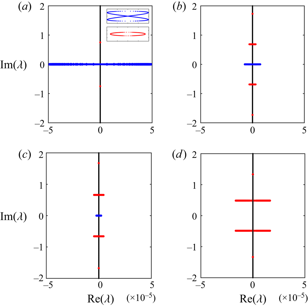
In figure 2, we use the Floquet–Fourier–Hill (FFH) method (Deconinck & Kutz Reference Deconinck and Kutz2006; Curtis & Deconinck Reference Curtis and Deconinck2010) to compute stability spectra of  $2{\rm \pi}$-periodic Stokes waves with amplitude
 $\varepsilon = 0.01$ in various depths. When
 $\kappa h > 1.3627\dots$, we observe the Benjamin–Feir instability as a figure-eight pattern at the origin. We also find unstable eigenvalues away from the origin, referred to as high-frequency instabilities. Unlike the Benjamin–Feir instability, high-frequency instabilities appear in the stability spectrum for all values of
 $\kappa h$. They even dominate the Benjamin–Feir instability when
 $1.3627\ldots <\kappa h < 1.4305\dots$ (Deconinck & Oliveras Reference Deconinck and Oliveras2011). The focus of this paper is on the study of these high-frequency instabilities using formal perturbation methods, as described below.
The stability spectrum of a  $2{\rm \pi}$-periodic Stokes wave with amplitude
 $\varepsilon = 0.01$ and (a)
 $h = \infty$, (b)
 $h=1.5$, (c)
 $h=1.4$ and (d)
 $h=1$. The Benjamin–Feir figure eight is coloured blue. The high-frequency isolas are coloured red. Purely imaginary eigenvalues are coloured black. A zoom-in of the Benjamin–Feir and high-frequency instabilities are inlaid in the top, left plot.

High-frequency instabilities develop from a Hamiltonian–Hopf bifurcation: a non-zero, repeated eigenvalue  $\lambda _0$ of the zero-amplitude stability spectrum (
 $\varepsilon =0$) leaves the imaginary axis as the amplitude increases (MacKay & Saffman Reference MacKay and Saffman1986; Akers & Nicholls Reference Akers and Nicholls2012; Deconinck & Trichtchenko Reference Deconinck and Trichtchenko2017). When
 $0<\varepsilon \ll 1$, a connected locus of unstable eigenvalues forms, which we call a high-frequency isola (red inset in figure 2). The isola is parameterized by values of
 $\mu$ near
 $\mu _0$, the Floquet exponent corresponding to
 $\lambda _0$.
High-frequency isolas are challenging to detect for numerical methods like FFH as they exist for narrow, specific ranges of the Floquet exponent. To complicate matters further, this narrow interval of Floquet exponents drifts from  $\mu _0$ as
 $\varepsilon$ increases. At most depths,
 $\mu _0$ is no longer within the interval that parameterizes the first high-frequency isola for small, positive values of
 $\varepsilon$. Therefore, to capture an isola using numerical methods, one must not only take into account the narrow interval of Floquet exponents that parameterizes the isola, but also its drift from
 $\mu _0$ as
 $\varepsilon$ changes (figure 3).
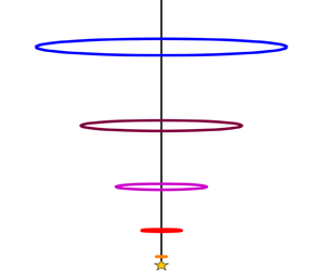
(a) The high-frequency isola closest to the origin for a  $2{\rm \pi}$-periodic Stokes wave in depth
 $h = 1.5$ with amplitude
 $\varepsilon = 2 \times 10^{-3}$ (orange),
 $\varepsilon = 4 \times 10^{-3}$ (red),
 $\varepsilon = 6 \times 10^{-3}$ (magenta),
 $\varepsilon = 8 \times 10^{-3}$ (purple) and
 $\varepsilon = 10^{-2}$ (blue). The imaginary axis is recentred to show the drift of the isola from the collided eigenvalues at
 $\lambda _0$. The isolas are computed using the perturbation method developed in this paper. (b) The interval of Floquet exponents that parameterizes the isola closest to the origin in depth
 $h=1.5$ as a function of the amplitude. The solid black lines indicate the boundaries of this interval, while the dashed black line gives the Floquet exponent corresponding to the most unstable eigenvalue on the isola. The coloured lines give the Floquet exponents corresponding to the similarly coloured isolas in the left figure. The Floquet axis is recentred to show the drift of the parameterizing interval from the Floquet exponent
 $\mu _0$ that corresponds to the collided eigenvalues. The parameterizing interval is also computed using the perturbation method in this paper.

In this paper, we derive formal asymptotic expressions for isolas close to the origin, both in finite and infinite depth. Specifically, for each isola we derive
(i) an interval of Floquet exponents that is asymptotic to the interval parameterizing the isola;
(ii) an asymptotic expansion for the most unstable eigenvalue on the isola; and
(iii) a closed-form expression for the curve asymptotic to the isola.
Our asymptotic expressions are compared directly with numerical results of the FFH method. For almost all  $\kappa h$ (except a few isolated values), our asymptotic expressions predict that Stokes waves of sufficiently small (but finite) amplitude are unstable with respect to high-frequency instabilities, extending recent work by Hur & Yang (Reference Hur and Yang2020) that establishes the instability closest to the origin only for
 $\kappa h\in (0.86430\dots, 1.00804\dots )$, see § 5.
Crucial to our approach is an expansion for the Floquet parameterization of the isola as power series in the wave amplitude  $\varepsilon$. This same approach was first used in Creedon, Deconinck & Trichtchenko (Reference Creedon, Deconinck and Trichtchenko2021a) on the Kawahara equation and in Creedon, Deconinck & Trichtchenko (Reference Creedon, Deconinck and Trichtchenko2021b) on a Boussinesq–Whitham system. An outline of the leading-order calculations of the method in infinite depth is also used by Akers (Reference Akers2015), where the emphasis is on understanding the analyticity properties of the stability spectrum as a function of the boundary conditions imposed on the perturbations (i.e. as a function of the Floquet exponent), and on the connections with resonant interaction theory.
2. The Ablowitz–Fokas–Musslimani formulation
Euler's equations (1.1a)–(1.1d) together with the auxiliary conditions (1.2a)–(1.2b) constitute a boundary value problem for Laplace's equation in a domain evolving nonlinearly in time. Depending on the application, other formulations of gravity waves may be preferred over (1.1a)–(1.1d). We consider the Ablowitz–Fokas–Musslimani (AFM) formulation, first proposed in Ablowitz et al. (Reference Ablowitz, Fokas and Musslimani2006). This formulation has dependence only on surface variables, as in Zakharov (Reference Zakharov1968) or Craig & Sulem (Reference Craig and Sulem1993), but avoids direct numerical computations of the Dirichlet-to-Neumann operator.
As shown in Ablowitz & Haut (Reference Ablowitz and Haut2008) and Oliveras (Reference Oliveras2009), Euler's equations (1.1a)–(1.1d) with the lateral periodic boundary conditions (1.2a)–(1.2b) are equivalent to the following system for the surface variables  $\eta$ and
 $q = \phi (x,\eta,t)$:
 \begin{gather} \int_{-{\rm \pi}/\kappa}^{{\rm \pi}/\kappa} {\rm e}^{-{\rm i}\kappa m x}\left[\eta_t\cosh\left(\kappa m\left(\eta + h\right) \right) +{\rm i}q_x\sinh\left(\kappa m\left(\eta + h \right) \right) \right] {{\rm d}\kern0.06em x} = 0, \quad m \in \mathbb{Z} {\setminus} \{0\}, \end{gather}
 \begin{gather}q_t + \frac 12 q_x^{2} +g\eta - \frac{1}{2}\frac{\left(\eta_t +\eta_xq_x\right)^{2}}{1+\eta_x^{2}} = 0. \end{gather}
We call (2.1a) and (2.1b) the non-local and local equations of the AFM formulation, respectively.
We write (2.1a)–(2.1b) in a travelling frame  $x \rightarrow x -ct$
 \begin{gather} \int_{-{\rm \pi}/\kappa}^{{\rm \pi}/\kappa} {\rm e}^{-{\rm i}\kappa m x}\left[\left(\eta_t-c\eta_x\right)\cosh\left(\kappa m\left(\eta \!+\! h\right) \right) +{\rm i}q_x\sinh\left(\kappa m\left(\eta + h \right) \right) \right] {{\rm d}}x \!=\! 0, \quad m \in \mathbb{Z} {\setminus} \{0\}, \end{gather}
 \begin{gather}q_t - cq_x + \frac 12 q_x^{2} +g\eta - \frac{1}{2}\frac{\left(\eta_t-c\eta_x +\eta_xq_x\right)^{2}}{1+\eta_x^{2}} = 0. \end{gather}
Unless otherwise stated,  $x$ represents the horizontal coordinate in the travelling frame for the remainder of this work.
Non-dimensionalizing (2.2a)–(2.2b) according to  $x \rightarrow x/\kappa$,
 $t \rightarrow t/\sqrt {g\kappa }$,
 $\eta \rightarrow \eta /\kappa$,
 $q \rightarrow q\sqrt {g/\kappa ^{3}}$,
 $c \rightarrow c\sqrt {g/\kappa }$ and
 $h \rightarrow \alpha /\kappa$, we arrive at
 \begin{gather} \int_{-{\rm \pi}}^{\rm \pi} {\rm e}^{-{\rm i} m x}\left[\left(\eta_t-c\eta_x\right)\cosh\left( m\left(\eta + \alpha\right) \right) +{\rm i}q_x\sinh\left(m\left(\eta + \alpha \right) \right) \right] {{\rm d}\kern0.06em x} = 0, \quad m \in \mathbb{Z} {\setminus} \{0\}, \end{gather}
 \begin{gather}q_t - cq_x + \frac{1}{2} q_x^{2} +\eta - \frac{1}{2}\frac{\left(\eta_t-c\eta_x +\eta_xq_x\right)^{2}}{1+\eta_x^{2}} = 0, \end{gather}
where  $\alpha = \kappa h >0$ is the aspect ratio of the surface profile
 $\eta$ (in dimensional variables). Without loss of generality, we study solutions of the non-dimensional equations (2.3a)–(2.3b).
Remark 2.1 Dividing ( 2.3 a) by  $\cosh ( m \alpha )$ and taking the limit
 $\alpha \rightarrow \infty$ yields (after some manipulation) the non-local equation in infinite depth
 \begin{equation} \int_{-{\rm \pi}}^{\rm \pi} \exp({-{\rm i} m x +|m|\eta}) \left[\eta_t-c\eta_x + {\rm i\,sgn}\left( m\right) q_x \right] {{\rm d}\kern0.06em x} = 0, \quad m \in \mathbb{Z} {\setminus} \{0\}. \end{equation}
The local equation remains unchanged in infinite depth.
3. Small-amplitude Stokes waves
Using the non-dimensional AFM formulation (2.3a)–(2.3b), Stokes waves are defined as surface displacements  $\eta _S$ and velocity potentials (at the surface)
 $q_S$ that satisfy the following:
(i)
 $\eta _S$ and $q_S$ are time-independent, infinitely smooth solutions of (2.3a)–(2.3b).
(ii)
$\eta _S$ and $q_{S,x}$ are $2{\rm \pi}$-periodic with respect to $x$ (but not so of $q_S$).(iii)
$\eta _S$, $q_{S,x}$ and $c$ (the velocity of the Stokes wave) depend analytically on a small parameter $\varepsilon$ such that
(3.1)\begin{equation} \left.\eta_S\right|_{\varepsilon =0} = 0 = \left.q_{S,x}\right|_{\varepsilon =0} \quad \textrm{and} \quad ||\eta_S||_{{L}^{2}} = \varepsilon + {O}\left(\varepsilon^{2}\right) \quad \textrm{as} \ \varepsilon \rightarrow 0. \end{equation}(iv)
$\eta _S$ and $q_{S,x}$ are even in $x$ without loss of generality, and $c(\varepsilon )$ is even in $\varepsilon$.(v)
$\eta _S$ has zero average over one period.


As mentioned in the Introduction, the existence of these waves is proven in Levi-Civita (Reference Levi-Civita1925), Nekrasov (Reference Nekrasov1921) and Struik (Reference Struik1926). In this section, we derive power series expansions of  $\eta _S$,
 $q_{S,x}$ and
 $c$ in the small parameter
 $\varepsilon$ using the non-dimensional AFM formulation. These expansions are required for the stability calculations considered in §§ 5 and 6.
Equating time derivatives to zero in (2.3a)–(2.3b) by property (i), integrating the  $\cosh$ term in (2.3a) by parts using property (ii) and solving for
 $q_x$ in (2.3b), we arrive at the following equations determining the Stokes waves:
 \begin{gather} \int_{-{\rm \pi}}^{\rm \pi} {\rm e}^{-{\rm i}mx}\sqrt{\left(1+\eta_{S,x}^{2}\right)\left(c^{2} - 2\eta_S \right)} \sinh(m(\eta_S+\alpha))\, {{\rm d}\kern0.06em x} = 0, \quad m \in \mathbb{Z} {\setminus} \{0\}, \end{gather}
 \begin{gather}q_{S,x} = c \pm \sqrt{\left(1+\eta_{S,x}^{2}\right)\left(c^{2} - 2\eta_S \right)}. \end{gather}
By property (iii), the positive branch of (3.2b) is defined for left-travelling waves ( $c<0$), while the negative branch is defined for right-travelling waves (
 $c>0$) (Constantin & Strauss Reference Constantin and Strauss2010). In what follows, we consider right-travelling waves. Similar results hold for the other case.
Remark 3.1 In infinite depth, ( 3.2 a) becomes
 \begin{equation} \int_{-{\rm \pi}}^{\rm \pi} \exp({-{\rm i}mx+|m|\eta_S})\sqrt{\left(1+\eta_{S,x}^{2}\right)\left(c^{2} - 2\eta_S \right)}\, {{\rm d}\kern0.06em x} = 0, \quad m \in \mathbb{Z} {\setminus} \{0\}. \end{equation}
By properties (ii) and (iv),  $\eta _S$ has a Fourier cosine series. We define the small-amplitude parameter
 $\varepsilon$ as the first Fourier cosine mode of
 $\eta _S$
 \begin{equation} \varepsilon=\frac{1}{\rm \pi}\int_{-{\rm \pi}}^{\rm \pi} \eta_S \cos(x)\, {{\rm d}\kern0.06em x}. \end{equation}
Then, by property (iii),
 \begin{equation} \eta_S(x;\varepsilon) = \varepsilon \cos(x) + {O}\left(\varepsilon^{2}\right), \end{equation}
for  $|\varepsilon |\ll 1$. The leading-order term of
 $\eta _S$ completely resolves the first Fourier cosine mode: higher-order corrections do not include terms proportional to
 $\cos (x)$ as a result.
Using properties (iii) and (iv), we write  $\eta _S$ and
 $c$ as power series in
 $\varepsilon$
 \begin{gather} \eta_S(x;\varepsilon) = \sum_{j=1}^{\infty} \eta_j(x)\varepsilon^{j}, \end{gather}
 \begin{gather}c(\varepsilon) = \sum_{j=0}^{\infty} c_{2j}\varepsilon^{2j}. \end{gather}
Both of these series are substituted into ( 3.2 a) and, after equating powers of  $\varepsilon$, a triangular sequence of linear integral equations for
 $\eta _j(x)$ and
 $c_{2j}$ is found. Each of these integral equations depends on
 $m$, which can be any non-zero integer.
Remark 3.2 Since  $\eta _S$ is even in
 $x$, the integrand of ( 3.2 a) modulo the complex exponential is even in
 $x$. Therefore,
 $m\in \mathbb {Z}^{+}$ without loss of generality.
The first non-trivial integral equation in this sequence is
 \begin{equation} \int_{-{\rm \pi}}^{\rm \pi}{\rm e}^{-{\rm i}mx}\left[mc_0^{2}\cosh(m\alpha)-\sinh(m\alpha) \right]\eta_1(x) \,{{\rm d}\kern0.06em x} = 0. \end{equation}
From above,  $\eta _1(x) = \cos (x)$. If ( 3.8) holds for all
 $m \in \mathbb {Z}^{+}$,
 \begin{equation} c_0^{2} = \tanh(\alpha), \end{equation}
otherwise ( 3.8) is not satisfied when  $m=1$. Since we study right-travelling waves, we choose
 $c_0>0$.
For the  $j{\textrm {th}}$ integral equation in the sequence (
 $j \geq 2$), one finds
 \begin{gather} \eta_{j}(x) = \sum_{\substack{\ell = 2 \\\ell\ \textrm{even}}}^{j}\hat{N}_{j,\ell}\cos(\ell x) \quad \textrm{for} \ j\ \textrm{even}, \end{gather}
 \begin{gather}\eta_{j}(x) = \sum_{\substack{\ell = 3 \\\ell\ \textrm{odd}}}^{j}\hat{N}_{j,\ell}\cos(\ell x) \quad \textrm{for} \ j\ \textrm{odd}, \end{gather}
where the coefficients  $\hat {N}_{j,\ell }$ are determined by the
 $j{\textrm {th}}$ equation with
 $m = \ell$. No corrections to the velocity
 $c$ are found when
 $j$ is even. When
 $j$ is odd,
 $c_{j-1}$ is determined by the
 $j{\textrm {th}}$ equation with
 $m = 1$, similar to the
 $j=1$ case considered above. This correction is chosen so that
 $\eta _j(x)$ has no terms proportional to
 $\cos (x)$.
Expansions of  $\eta _S$ and
 $c$ are substituted into (3.2b). After equating powers of
 $\varepsilon$, an expansion for
 $q_{S,x}$ follows immediately. In general,
 \begin{equation} q_{S,x}(x;\varepsilon) = \sum_{j=1}^{\infty} q_{j,x}(x)\varepsilon^{j}. \end{equation}
The corrections  $q_{j,x}(x)$ have the same structure as (3.10a)–(3.10b), but also include constant modes (when
 $j$ is even) and modes proportional to
 $\cos (x)$ (when
 $j$ is odd). Thus,
 $q_{S,x}$ has non-zero average, and the first Fourier cosine mode of
 $q_{S,x}$ has corrections beyond
 ${O}(\varepsilon )$, unlike
 $\eta _S$.
Remark 3.3 Integrating ( 3.11) term-by-term gives  $q_S$. The constant of integration can be eliminated by a Galilean transformation of ( 3.2 b). Because
 $q_{S,x}$ has non-zero average,
 $q_S$ exhibits linear growth in
 $x$. This behaviour captures the mean flow induced by the travelling frame.
Explicit representations for the expansions of  $\eta _S$,
 $q_{S,x}$ and
 $c$ up to
 ${O}(\varepsilon ^{4})$ are found in Appendix A. In figure 4, these expansions show excellent agreement with direct numerical computations of the Stokes waves using the continuation method presented in Deconinck & Oliveras (Reference Deconinck and Oliveras2011).
(a) The amplitude vs velocity bifurcation diagram of  $2{\rm \pi}$-periodic Stokes waves when
 $\alpha = 1$ (dashed line),
 $\alpha = 1.5$ (dotted line),
 $\alpha = 2$ (dot-dashed line) and
 $\alpha = \infty$ (solid line), according to our
 ${O}(\varepsilon ^{4})$ asymptotic calculations. The zeroth-order contribution
 $c_0$ is removed for better visibility. The numerical results are given by the coloured dots. Red dots correspond to
 $\alpha = 1$, magenta dots correspond to
 $\alpha = 1.5$, purple dots correspond to
 $\alpha = 2$ and blue dots correspond to
 $\alpha = \infty$. (b) Expansions of
 $\eta _S/\varepsilon$ to
 ${O}(\varepsilon ^{4})$ with
 $\varepsilon = 0.1$ for
 $\alpha = 1, 1.5, 2$ and
 $\infty$ (arranged from top to bottom using the same line styles as in panel a). A sampling of the numerical results is given by the coloured dots using the same colour scheme as in panel (a).

4. The spectral instability of Stokes waves
4.1. The stability spectrum
We consider perturbations to the Stokes waves of the form
 \begin{equation} \begin{pmatrix} \eta(x,t;\varepsilon,\rho) \\ q(x,t;\varepsilon,\rho) \end{pmatrix} = \begin{pmatrix} \eta_S(x;\varepsilon) \\ q_S(x;\varepsilon) \end{pmatrix} + \rho \begin{pmatrix} \eta_\rho(x,t; \varepsilon) \\ q_\rho(x,t; \varepsilon) \end{pmatrix} + {O}\left(\rho^{2}\right), \end{equation}
where  $|\rho |\ll 1$ is a parameter independent of
 $\varepsilon$. The perturbations
 $\eta _\rho$ and
 $q_\rho$ are sufficiently smooth functions of
 $x$ and
 $t$ that are bounded over the real line for each
 $t\geq 0$.
The non-local equation (2.3a) assumes  $\eta$,
 $\eta _t$ and
 $q_x$ are
 $2{\rm \pi}$-periodic in
 $x$, which is not required of our perturbations. We modify (2.3a) to allow
 $\eta, \eta _t$ and
 $q_x \in C^{0}(\mathbb {R}) \cap L^{\infty }(\mathbb {R})$ for each
 $t \geq 0$. The appropriate modification is
 \begin{equation} \left\langle {\rm e}^{-{\rm i} k x}\left[\left(\eta_t-c\eta_x\right)\cosh\left(k\left(\eta + \alpha \right) \right) +{\rm i}q_x\sinh\left(k\left(\eta + \alpha \right) \right) \right] \right\rangle = 0, \quad k \in \mathbb{R} {\setminus} \{0\}, \end{equation}
where
 \begin{equation} \left\langle f(x) \right\rangle = \displaystyle \lim_{L \rightarrow \infty} \frac{1}{L} \int_{{-}L/2}^{L/2} f(x) \,{{\rm d}\kern0.06em x}, \end{equation}
for any  $f(x) \in C^{0}(\mathbb {R}) \cap L^{\infty }(\mathbb {R})$ (Bohr Reference Bohr1947; Deconinck & Oliveras Reference Deconinck and Oliveras2011). If
 $\eta, \eta _t$ and
 $q_x$ are
 $2{\rm \pi}$-periodic in
 $x$ for each
 $t\geq 0$, then (4.2) reduces to (2.3a).
Substituting (4.1) into (2.3b) and (4.2) and equating powers of  $\rho$, terms of
 ${O}(\rho ^{0})$ necessarily cancel, since
 $\eta _S$ and
 $q_S$ solve (2.3b) and (4.2). At
 ${O}(\rho )$, one finds the governing equations for
 $\eta _\rho$ and
 $q_\rho$
 \begin{gather} \left\langle {\rm e}^{-{\rm i}kx}\left[c\mathcal{C}_k\eta_{\rho,x} +k\left(c\mathcal{S}_k\eta_{S,x} -{\rm i} \mathcal{C}_kq_{S,x} \right)\eta_\rho -{\rm i}\mathcal{S}_kq_{\rho,x}\right] \right\rangle = \left\langle {\rm e}^{-{\rm i}kx}\mathcal{C}_k\eta_{\rho,t} \right\rangle, \end{gather}
 \begin{gather}\eta_{S,x}{\zeta}^{2}\eta_{\rho,x} - \eta_{\rho} -{\zeta}q_{\rho,x} = q_{\rho,t} -\eta_{S,x}{\zeta}\eta_{\rho,t}, \end{gather}
where
 \begin{equation} \mathcal{C}_k = \cosh(k(\eta_S+\alpha)), \quad \mathcal{S}_k = \sinh(k(\eta_S+\alpha)), \quad {\zeta} =\frac{q_{S,x}- c}{1+\eta_{S,x}^{2}}. \end{equation}
Equations (4.4a)–(4.4b) are autonomous in  $t$. We separate variables to find
 \begin{equation} \begin{pmatrix} \eta_\rho(x,t) \\ q_\rho(x,t) \end{pmatrix} = {\rm e}^{\lambda t}\begin{pmatrix} N(x) \\ Q(x) \end{pmatrix}, \end{equation}
where  $\lambda \in \mathbb {C}$ controls the growth rates of the perturbations. The functions
 $N(x)$ and
 $Q(x)$ satisfy
 \begin{gather} \left\langle {\rm e}^{-{\rm i}kx}\left[c\mathcal{C}_kN_x +k\left(c\mathcal{S}_k\eta_{S,x} -{\rm i}\mathcal{C}_kq_{S,x} \right)N -{\rm i}\mathcal{S}_kQ_x\right] \right\rangle = \lambda \left\langle {\rm e}^{-{\rm i}kx}\mathcal{C}_kN \right\rangle, \end{gather}
 \begin{gather}\eta_{S,x}{\zeta}^{2}N_x - N -{\zeta}Q_x = \lambda\left(Q -\eta_{S,x}{\zeta}N\right). \end{gather}
Equations (4.7a)–(4.7b) are invariant under the shift  $x \rightarrow x + 2{\rm \pi}$ by the periodicity of
 $\eta _S$ and
 $q_{S,x}$. Therefore, we expect the solutions
 $N$ and
 $Q$ to have Bloch form (Deconinck & Oliveras Reference Deconinck and Oliveras2011)
 \begin{equation} \begin{pmatrix} N(x) \\ Q(x) \end{pmatrix} = {\rm e}^{{\rm i}\mu x}\begin{pmatrix} \mathcal{N}(x) \\ \mathcal{Q}(x) \end{pmatrix}, \end{equation}
where  $\mu \in \mathbb {R}$ is the Floquet exponent and
 $\mathcal {N}$ and
 $\mathcal {Q}$ are sufficiently smooth and
 $2{\rm \pi}$-periodic. Note that by redefining
 $\mathcal {N}$ and
 $\mathcal {Q}$,
 $\mu \in [-1/2,1/2)$, without loss of generality.
Substituting (4.8) into (4.7a)–(4.7b), we arrive at
 \begin{align} &\left\langle \exp({-{\rm i}(k-\mu)x})\left[c\mathcal{C}_k\mathcal{D}_x\mathcal{N} +k\left( c\mathcal{S}_k\eta_{S,x} -{\rm i}\mathcal{C}_kq_{S,x} \right)\mathcal{N} -{\rm i}\mathcal{S}_k \mathcal{D}_x\mathcal{Q} \right] \right\rangle \nonumber\\ &\quad = \lambda \left\langle \exp({-{\rm i}(k-\mu)x})\mathcal{C}_k\mathcal{N} \right\rangle, \end{align}
 \begin{gather} \eta_{S,x}{\zeta}^{2}\mathcal{D}_x\mathcal{N} - \mathcal{N} -{\zeta}\mathcal{D}_x\mathcal{Q} = \lambda\left(\mathcal{Q} -\eta_{S,x}{\zeta}\mathcal{N}\right) ,\end{gather}
where  $\mathcal {D}_x = {\rm i}\mu + \partial _x$.
The integrands of the averaging operators in (4.9a) are  $2{\rm \pi}$-periodic except for the complex exponentials. These operators evaluate to zero unless
 $k-\mu = n \in \mathbb {Z}$ (Deconinck & Oliveras Reference Deconinck and Oliveras2011). For such
 $k$, (4.9a) becomes
 \begin{align} &\left\langle {\rm e}^{-{\rm i}nx}\left[c\mathcal{C}_{n+\mu}\mathcal{D}_x\mathcal{N} +(n+\mu)\left(c\mathcal{S}_{n+\mu}\eta_{S,x} -{\rm i}\mathcal{C}_{n+\mu}q_{S,x} \right)\mathcal{N} -{\rm i}\mathcal{S}_{n+\mu}\mathcal{D}_x\mathcal{Q} \right] \right\rangle \nonumber\\ &\quad = \lambda \left\langle {\rm e}^{-{\rm i}nx}\mathcal{C}_{n+\mu}\mathcal{N} \right>, \quad n \in \mathbb{Z}. \end{align}
The averaging operators of (4.10) reduce to Fourier transforms
 \begin{equation} \left\langle {\rm e}^{-{\rm i}nx}f(x)\right\rangle = \frac{1}{2{\rm \pi}}\int_{-{\rm \pi}}^{\rm \pi} {\rm e}^{-{\rm i}nx} f(x) \,{{\rm d}\kern0.06em x} = \mathcal{F}_n[f(x)], \end{equation}
for any  $f(x) \in L^{2}_{{per}}(-{\rm \pi},{\rm \pi} )$. The inverse transform is
 \begin{equation} \mathcal{F}^{{-}1}[\{f_n\}] = \sum_{n={-}\infty}^{\infty} f_n {\rm e}^{{\rm i}nx}, \end{equation}
provided  $\{f_n\} \in \ell ^{2}(\mathbb {Z})$. Using the inverse transform on (4.10), we find
 \begin{align} &\sum_{n={-}\infty}^{\infty}{\rm e}^{{\rm i}nx}\mathcal{F}_n\left[c\mathcal{C}_{n+\mu}\mathcal{D}_x\mathcal{N} +(n+\mu)\left(c\mathcal{S}_{n+\mu}\eta_{S,x} -{\rm i}\mathcal{C}_{n+\mu}q_{S,x} \right)\mathcal{N} \right] \nonumber\\ &\quad+ \sum_{n={-}\infty}^{\infty}{\rm e}^{{\rm i}nx}\mathcal{F}_n\left[-{\rm i}\mathcal{S}_{n+\mu}\mathcal{D}_x\mathcal{Q} \right]=\lambda \sum_{n={-}\infty}^{\infty}{\rm e}^{{\rm i}nx}\mathcal{F}_n\left[\mathcal{C}_{n+\mu}\mathcal{N} \right]. \end{align}
Equations (4.9b) and (4.13) are written compactly as
 \begin{equation} \mathcal{L}_{\mu,\varepsilon} \boldsymbol{w}_{\mu,\varepsilon} = \lambda_{\mu,\varepsilon} \mathcal{R}_{\mu,\varepsilon} \boldsymbol{w}_{\mu,\varepsilon},\end{equation}
where  $\lambda _{\mu,\varepsilon }=\lambda $,
 $\boldsymbol {w}_{\mu,\varepsilon } = (\mathcal {N},\mathcal {Q})^{\rm T}$ and
 \begin{equation} \mathcal{L}_{\mu,\varepsilon} = \begin{pmatrix} \mathcal{L}_{\mu,\varepsilon}^{(1,1)} & \mathcal{L}_{\mu,\varepsilon}^{(1,2)} \\ \mathcal{L}_{\mu,\varepsilon}^{(2,1)} & \mathcal{L}_{\mu,\varepsilon}^{(2,2)} \end{pmatrix}, \quad \mathcal{R}_{\mu,\varepsilon} = \begin{pmatrix} \mathcal{R}_{\mu,\varepsilon}^{(1,1)} & 0 \\ \mathcal{R}_{\mu,\varepsilon}^{(2,1)} & 1 \end{pmatrix}, \end{equation}
 \begin{gather} \mathcal{L}_{\mu,\varepsilon}^{(1,1)}[\mathcal{N}] = \sum_{n={-}\infty}^{\infty}{\rm e}^{{\rm i}nx} \mathcal{F}_n \left[c\mathcal{C}_{n+\mu} \mathcal{D}_x\mathcal{N} +(n+\mu)\left(c\mathcal{S}_{n+\mu}\eta_{S,x} -{\rm i}\mathcal{C}_{ n+\mu}q_{S,x} \right)\mathcal{N}\right], \end{gather}
 \begin{gather}\mathcal{L}_{\mu,\varepsilon}^{(1,2)}[\mathcal{Q}] = \sum_{n={-}\infty}^{\infty}{\rm e}^{{\rm i}nx}\mathcal{F}_n\left[-{\rm i}\mathcal{S}_{n+\mu}\mathcal{D}_x \mathcal{Q} \right], \end{gather}
 \begin{gather}\mathcal{L}_{\mu,\varepsilon}^{(2,1)}[\mathcal{N}] = \eta_{S,x}{\zeta}^{2}\mathcal{D}_x\mathcal{N} - \mathcal{N}, \end{gather}
 \begin{gather}\mathcal{L}_{\mu,\varepsilon}^{(2,2)}[\mathcal{Q}] ={-}{\zeta}\mathcal{D}_x\mathcal{Q}, \end{gather}
 \begin{gather}\mathcal{R}_{\mu,\varepsilon}^{(1,1)}[\mathcal{N}] = \sum_{n={-}\infty}^{\infty}{\rm e}^{{\rm i}nx} \mathcal{F}_n\left[\mathcal{C}_{n+\mu}\mathcal{N} \right], \end{gather}
 \begin{gather}\mathcal{R}_{\mu,\varepsilon}^{(2,1)}[\mathcal{N}] ={-}\eta_{S,x}{\zeta}\mathcal{N}. \end{gather}
Equation (4.14) represents a two-parameter family of generalized eigenvalue problems for the linear operators  $\mathcal {L}_{\mu,\varepsilon }$ and
 $\mathcal {R}_{\mu,\varepsilon }$.
Remark 4.1 In infinite depth,
 \begin{gather} \mathcal{L}_{\mu,\varepsilon}^{(1,1)}[\mathcal{N}] = \sum_{n={-}\infty}^{\infty} {\rm e}^{{\rm i}nx}\mathcal{F}_n\left[{\rm e}^{|n+\mu|\eta_S}\left( c\mathcal{D}_x\mathcal{N} +\left(c\eta_{S,x}|n+\mu|-{\rm i}(n+\mu)q_{S,x}\right)\mathcal{N} \right) \right], \end{gather}
 \begin{gather}\mathcal{L}_{\mu,\varepsilon}^{(1,2)}[\mathcal{Q}] = \sum_{n={-}\infty}^{\infty} {\rm e}^{{\rm i}nx}\mathcal{F}_n\left[{\rm e}^{|n+\mu| \eta_S}\left( -{\rm i}\,\textrm{sgn}(n+\mu)\mathcal{D}_x\mathcal{Q} \right)\right], \end{gather}
 \begin{gather}\mathcal{R}_{\mu,\varepsilon}^{(1,1)}[\mathcal{N}] = \sum_{n={-}\infty}^{\infty} {\rm e}^{{\rm i}nx}\mathcal{F}_n\left[{\rm e}^{|n+\mu| \eta_S}\mathcal{N}\right]. \end{gather}
All other entries are the same as above.
The spectrum of (4.14) has a countable collection of finite-multiplicity eigenvalues  $\lambda _{\mu,\varepsilon }$ for each
 $\mu$ (Deconinck & Oliveras Reference Deconinck and Oliveras2011; Kapitula & Promislow 2013; Akers & Nicholls Reference Akers and Nicholls2014). The union of these eigenvalues over
 $\mu \in [-1/2,1/2)$ is defined as the stability spectrum of Stokes waves with amplitude
 $\varepsilon$. If there exists
 $\lambda _{\mu,\varepsilon }$ for some
 $\mu$ such that
 ${\rm Re}(\lambda _{\mu,\varepsilon } )>0$, then there exist perturbations of the Stokes waves
 $\eta _{\rho }$ and
 $q_{\rho }$ that grow exponentially in time. In this case, the Stokes waves are spectrally unstable. If no such
 $\mu$ and
 $\lambda _{\mu,\varepsilon }$ exist, the Stokes waves are spectrally stable.
4.2. Necessary conditions for high-frequency instabilities
When  $\varepsilon =0$, (4.14) reduces to a generalized eigenvalue problem with constant coefficients
 \begin{equation} {\small\begin{pmatrix} {\rm i}c_0(\mu+D)\cosh(\alpha(\mu+D)) & (\mu+D)\sinh(\alpha(\mu+D)) \\ -1 & {\rm i}c_0(\mu+D) \end{pmatrix} \boldsymbol{w}_{\mu,0} = \lambda_{\mu,0}\begin{pmatrix} \cosh(\alpha(\mu+D)) & 0 \\ 0 & 1 \end{pmatrix}\boldsymbol{w}_{\mu,0},} \end{equation}
where  $D=-{\rm i}\partial _x$. The eigenvalues of (4.18) are
 \begin{equation} \lambda_{\mu,0,n}^{(\sigma)} ={-}{\rm i}\varOmega_{\sigma}(\mu+n), \quad \sigma ={\pm} 1, \quad n \in \mathbb{Z},\end{equation}
with
 \begin{gather} \varOmega_{\sigma}(z) ={-}c_0z +\sigma \omega(z), \end{gather}
 \begin{gather}\omega(z) = \textrm{sgn}(z)\sqrt{z\tanh(\alpha z)}. \end{gather}
Equation (4.20a) is the linear dispersion relation of the non-dimensional Euler equations in a frame travelling with velocity  $c_0$. The parameter
 $\sigma$ specifies the branch of the dispersion relation. As expected, (4.19) gives a countable collection of eigenvalues for each
 $\mu \in [-1/2,1/2)$. These eigenvalues are purely imaginary, and therefore, the zero-amplitude Stokes waves are spectrally stable.
High-frequency instabilities develop from non-zero eigenvalues of (4.18) that have double (algebraic and geometric) multiplicity for a Floquet exponent  $\mu _0$ that satisfies (MacKay & Saffman Reference MacKay and Saffman1986; Akers & Nicholls Reference Akers and Nicholls2012; Deconinck & Trichtchenko Reference Deconinck and Trichtchenko2017)
 \begin{equation} \lambda^{(\sigma_1)}_{\mu_0,0,n} = \lambda^{(\sigma_2)}_{\mu_0,0,n+p} \neq 0,\end{equation}
for  $p \in \mathbb {Z} {\setminus} \{0\}$. Such double eigenvalues occur only if
 $\sigma _1 \neq \sigma _2$ and
 $|p|>1$ (Deconinck & Trichtchenko Reference Deconinck and Trichtchenko2017). More specifically, we have the following theorem:
Theorem 4.2 Let  $c_0>0$,
 $\sigma _1 = 1$ and
 $\sigma _2 = -1$. For each
 $p \in \mathbb {Z} {\setminus} \{0,\pm 1\}$, there exists a unique Floquet exponent
 $\mu _{0,p} \in [-1/2,1/2)$ and unique integer
 $n_p$ such that
 \begin{equation} \lambda_{0,p} = \lambda^{(1)}_{\mu_{0,p},0,n_p} = \lambda^{({-}1)}_{\mu_{0,p},0,n_p+p} \neq 0. \end{equation}
The eigenvalues have the symmetry  $\lambda _{0,-p} = -\lambda _{0,p}$, and the magnitudes of the eigenvalues are strictly monotonically increasing as
 $|p| \rightarrow \infty$. The corresponding eigenfunctions are
 \begin{equation} \boldsymbol{w}_{0,p} = \beta_0 \begin{pmatrix} 1 \\ \dfrac{-{\rm i}}{\omega(n_p+\mu_{0,p})} \end{pmatrix} \exp({{\rm i}n_px}) + \gamma_0 \begin{pmatrix} 1 \\ \dfrac{{\rm i}}{\omega(n_p+p+\mu_{0,p})} \end{pmatrix} \exp({{\rm i}(n_p+p)x}), \end{equation}
where  $\omega$ is given by (4.20b) and
 $\beta _0,\gamma _0 \in \mathbb {C} {\setminus} \{0\}$.
An important corollary is the following:
Corollary 4.3 Let  $c_0>0$. Let
 $\lambda _{0,p}$ be given by (4.22) for some
 $p \in \mathbb {Z} {\setminus} \{0,\pm 1\}$. Then,
 \begin{equation} \omega(n_p+\mu_{0,p})\omega(n_p+p+\mu_{0,p})>0, \end{equation}
and
 \begin{equation} c_{g,1}(n_p+\mu_{0,p}) \neq c_{g,-1}(n_p+p+\mu_{0,p}), \end{equation}
where  $c_{g,\sigma }(z)$ is the group velocity of
 $\varOmega _{\sigma }(z)$, i.e.
 $c_{g,\sigma }(z) = \varOmega _{\sigma,z}(z).$
Similar results hold if  $c_0<0$ provided
 $\sigma _1 = -1$ and
 $\sigma _2 = 1$. See Creedon et al. (Reference Creedon, Deconinck and Trichtchenko2021b) for the proofs of Theorem 4.2 and Corollary 4.3.
The product (4.24) is equivalent to the Krein condition developed by MacKay & Saffman (Reference MacKay and Saffman1986) and, in more generality, Deconinck & Trichtchenko (Reference Deconinck and Trichtchenko2017). This is a second necessary condition for the development of high-frequency instabilities. Corollary 4.3 guarantees this condition is satisfied for all non-zero eigenvalues of (4.18) with double multiplicity. Both (4.24) and (5.3) are crucial to the formal asymptotic expansions of the high-frequency instabilities derived in §§ 5 and 6.
Remark 4.4 In infinite depth,  $\mu _{0,p}$ and
 $\lambda _{0,p}$ are known explicitly. For
 $c_0>0$,
 \begin{gather} \mu_{0,p} ={-}\frac{{\rm{sgn}}{(p)}}{8}\left(({-}1)^{p}+1\right), \end{gather}
 \begin{gather}\lambda_{0,p} = {\rm i}\frac{{\rm {sgn}}(p)}{4}\left(1-p^{2}\right). \end{gather}
These eigenvalues have the conjugate symmetry  $\lambda _{0,-p} = -\lambda _{0,p}$, and
 $\{|\lambda _{0,p}|\}$ is strictly monotonically increasing as
 $|p| \rightarrow \infty$, similar to the finite-depth case.
5. First isola. High-frequency instabilities: $p=2$

We develop a perturbation method to obtain the leading-order behaviour of the high-frequency isola that arises from  $\lambda _{0,p}$ with
 $p=2$. According to Theorem 4.2, this isola is the closest to the origin. We assume the spectral data of (4.14) corresponding to the isola vary analytically with
 $\varepsilon$, including the Floquet exponent
 \begin{gather} \lambda_{\mu(\varepsilon),\varepsilon} = \lambda_{0,p} + \lambda_1 \varepsilon+ \lambda_2 \varepsilon^{2} +{O}\left(\varepsilon^{3}\right), \end{gather}
 \begin{gather}\boldsymbol{w}_{\mu(\varepsilon),\varepsilon} = \boldsymbol{w}_{0,p} + \boldsymbol{w}_1 \varepsilon + \boldsymbol{w}_2 \varepsilon^{2} + {O}\left(\varepsilon^{3}\right), \end{gather}
 \begin{gather}\mu(\varepsilon) = \mu_{0,p} + \mu_1\varepsilon + \mu_2\varepsilon^{2} + {O}\left(\varepsilon^{3}\right). \end{gather}
If the Floquet exponent is fixed, at most two eigenvalues are found on the isola by standard eigenvalue perturbation theory (Kato Reference Kato1966). If instead the Floquet exponent is formally expanded in  $\varepsilon$, all of the eigenvalues on the isola can be approximated at once. We see below that the leading-order behaviour of these eigenvalues is obtained at
 ${O}(\varepsilon ^{2})$.
Remark 5.1 Choosing  $p=-2$ gives the isola conjugate to the
 $p=2$ isola. Thus, we choose
 $p=2$ without loss of generality.
We impose the following normalization on  $\boldsymbol {w}_{\mu (\varepsilon ),\varepsilon }$:
 \begin{equation} \mathcal{F}_{n_p}[\boldsymbol{w}_{\mu(\varepsilon),\varepsilon}\boldsymbol{\cdot}\boldsymbol{e}_1] = 1, \end{equation}
where  $n_p \in \mathbb {Z}$ is given by Theorem 4.2 and
 $\boldsymbol {e}_1 = (1,0)^{\rm T}$. Then,
 $\beta _0 = 1$ in (4.23), and all subsequent corrections of
 $\boldsymbol {w}_{\mu (\varepsilon ),\varepsilon }$ do not include the Fourier mode
 $\textrm {exp}(in_px)$ in the first component. The eigenvalue and Floquet expansions, (5.1a) and (5.1c) above, are unaffected by this normalization. For ease of notation, let
 $\lambda _{0,p} \rightarrow \lambda _0$,
 $\boldsymbol {w}_{0,p} \rightarrow \boldsymbol {w}_0$,
 $\mu _{0,p} \rightarrow \mu _0$ and
 $n_p \rightarrow n$.
Several of the asymptotic expressions that follow are suppressed for ease of readability. See the Data Availability Statement at the end of this manuscript for access to the full expressions.
5.1. The ${O}(\varepsilon )$ problem

Substituting expansions (5.1a)–(5.1c) into the generalized eigenvalue problem (4.14) and equating powers of  $\varepsilon$, terms of
 ${O}(\varepsilon ^{0})$ cancel by the choice of
 $\lambda _{0}$,
 $\boldsymbol {w}_0$ and
 $\mu _0$. Terms of
 ${O}(\varepsilon )$ yield
 \begin{equation} \left(L_0-\lambda_{0}R_0\right)\boldsymbol{w}_1 = \left(\lambda_1R_0 - \left(L_1 - \lambda_{0} R_1 \right) \right)\boldsymbol{w}_0,\end{equation}
where
 \begin{equation} L_j =\left. \frac{1}{j!} \frac{\partial^{j}\mathcal{L}_{\mu(\varepsilon),\varepsilon}}{\partial \varepsilon^{j}}\right|_{\varepsilon = 0}, \quad R_j = \left.\frac{1}{j!} \frac{\partial^{j}\mathcal{R}_{\mu(\varepsilon),\varepsilon}}{\partial \varepsilon^{j}}\right|_{\varepsilon = 0}, \quad j \in \mathbb{W}. \end{equation}
If (5.3) can be solved for  $\boldsymbol {w}_1$, the inhomogeneous terms on the right-hand side of (5.3) must be orthogonal to the nullspace of the adjoint of
 $L_0-\lambda _{0}R_0$ by the Fredholm alternative. A direct calculation shows
 \begin{equation} \textrm{Null}\left(\left(L_0-\lambda_{0}R_0\right)^{{{\dagger}}}\right) = \textrm{Span}\left\{ \begin{pmatrix} 1 \\ -i\omega\left(n+\mu_0\right) \end{pmatrix} {\rm e}^{{\rm i}n x}, \begin{pmatrix} 1 \\ {\rm i}\omega\left(n+p+\mu_0\right) \end{pmatrix} {\rm e}^{{\rm i}(n+p)x} \right\}. \end{equation}
Hence, we impose the following solvability conditions on (5.3):
 \begin{gather} \left\langle \begin{pmatrix} 1 \\ -{\rm i}\omega\left(n+\mu_0\right) \end{pmatrix} {\rm e}^{{\rm i}n x}, \left(\lambda_1R_0 - \left(L_1 - \lambda_{0} R_1 \right) \right)\boldsymbol{w}_0\right\rangle = 0, \end{gather}
 \begin{gather}\left\langle\begin{pmatrix} 1 \\ {\rm i}\omega\left(n+p+\mu_0\right) \end{pmatrix} {\rm e}^{{\rm i}(n+p)x} , \left(\lambda_1R_0 - \left(L_1 - \lambda_{0} R_1 \right) \right)\boldsymbol{w}_0 \right\rangle = 0, \end{gather}
where  $\left \langle \cdot,\cdot \right \rangle$ is the standard inner product on
 ${L}^{2}_{{per}}(-{\rm \pi},{\rm \pi} )\times L^{2}_{{per}}(-{\rm \pi},{\rm \pi} )$. Simplifying both conditions, we arrive at
 \begin{gather} \lambda_1 + {\rm i}\mu_1c_{g,1}\left(n+\mu_0\right) = 0, \end{gather}
 \begin{gather}\gamma_0\left(\lambda_1 + {\rm i}\mu_1c_{g,-1}\left(n+p+\mu_0 \right)\right) = 0. \end{gather}
Since  $\gamma _0 \neq 0$ by Theorem 4.2 and
 $c_{g,1}(n+\mu _0) \neq c_{g,-1}(n+p+\mu _0 )$ by Corollary 4.3, we must have
 \begin{equation} \lambda_1 = 0 = \mu_1. \end{equation}
Thus no instabilities are found at  ${O}(\varepsilon )$.
Before proceeding to  ${O}(\varepsilon ^{2})$, we invert
 $L_0-\lambda _{0}R_0$ against its range to find the particular solution of
 $\boldsymbol {w}_1$. Uniting the particular solution with the nullspace of
 $L_0-\lambda _{0}R_0$,
 \begin{equation} \boldsymbol{w}_1 = \sum_{\substack{j = n-1 \\ j \neq n, n+p}}^{n+p+1} \hat{\mathcal{W}}_{1,j}{\rm e}^{{\rm i}jx} + \beta_1 \begin{pmatrix} 1 \\ \dfrac{-{\rm i}}{\omega(n+\mu_0)} \end{pmatrix} {\rm e}^{{\rm i}nx} + \gamma_1 \begin{pmatrix} 1 \\ \dfrac{{\rm i}}{\omega(n+p+\mu_0)} \end{pmatrix} {\rm e}^{{\rm i}(n+p)x}, \end{equation}
where the coefficients  $\hat {\mathcal {W}}_{1,j}$ depend on
 $\alpha$ (possibly through intermediate dependencies on known zeroth-order results) and at most linearly on
 $\gamma _0$. The parameter
 $\gamma _1 \in \mathbb {C}$ is free at this order. By our choice of normalization (5.2),
 $\beta _1 = 0$. Thus,
 \begin{equation} \boldsymbol{w}_1 = \sum_{\substack{j = n-1 \\ j \neq n, n+p}}^{n+p+1} \hat{\mathcal{W}}_{1,j}{\rm e}^{{\rm i}jx} + \gamma_1 \begin{pmatrix} 1 \\ \dfrac{{\rm i}}{\omega(n+p+\mu_0)} \end{pmatrix} {\rm e}^{{\rm i}(n+p)x}. \end{equation}
5.2. The ${O}(\varepsilon ^{2})$ problem

At  ${O}(\varepsilon ^{2})$, the spectral problem (4.14) is
 \begin{equation} \left(L_0 - \lambda_{0}R_0\right)\boldsymbol{w}_2 = \lambda_2 R_0\boldsymbol{w}_0 - \left(L_1 - \lambda_{0}R_1 \right)\boldsymbol{w}_1 - \left(L_2 - \lambda_{0}R_2\right)\boldsymbol{w}_0, \end{equation}
using (5.8). Proceeding as above, we obtain the solvability conditions for (5.11)
 \begin{gather} 2\left(\lambda_2 + {\rm i}\mathfrak{c}_{2,1,n}\right) + {\rm i}\gamma_0\mathfrak{s}_{2,n} = 0, \end{gather}
 \begin{gather}2\gamma_0\left(\lambda_2 + {\rm i}\mathfrak{c}_{2,-1,n+p}\right) + {\rm i} \mathfrak{s}_{2,n+p} = 0, \end{gather}
where
 \begin{equation} \mathfrak{c}_{2,\sigma,j} = \mu_2c_{g,\sigma}\left(j+\mu_0\right) - \mathfrak{p}_{2,j}. \end{equation}
The quantities  $\mathfrak {s}_{2,j}$ and
 $\mathfrak {p}_{2,j}$ depend only on
 $\alpha$ (possibly through known zeroth- and first-order quantities). Using the collision condition (4.21), it can be shown that the product of
 $\mathfrak {s}_{2,n}$ and
 $\mathfrak {s}_{2,n+p}$ is related to a perfect square:
 \begin{equation} \mathfrak{s}_{2,n} \mathfrak{s}_{2,n+p} ={-} \frac{\mathcal{S}_2^{2}}{ \omega(n+\mu_0)\omega(n+p+\mu_0)}, \end{equation}
where
 \begin{equation} \mathcal{S}_2 = \mathcal{T}_{2,1} + \mathcal{T}_{2,2}\hat{N}_{2,2} + \mathcal{T}_{2,3}\hat{Q}_{2,2}. \end{equation}
The expressions  $\mathcal {T}_{2,j}$ are functions only of
 $\alpha$, as are the Stokes wave corrections
 $\hat {N}_{2,2}$ and
 $\hat {Q}_{2,2}$, see Appendix A. When fully expanded,
 $\mathcal {S}_2$ consists of roughly 100 terms (depending on how it is written), but each term depends only on
 $\alpha$. The full expression of
 $\mathcal {S}_2$ is found in the appropriate Mathematica notebook provided in the Data Availability Statement.
Solving for  $\lambda _2$ in (5.12a)–(5.12b),
 \begin{equation} \lambda_2 ={-}{\rm i}\left(\frac{\mathfrak{c}_{2,-1,n+p} \!+\! \mathfrak{c}_{2,1,n}}{2} \right) \pm \sqrt{-\left(\frac{\mathfrak{c}_{2,-1,n\!+\!p} - \mathfrak{c}_{2,1,n}}{2} \right)^{2} \!+\! \frac{\mathcal{S}_2^{2}}{4\omega(n\!+\!\mu_0)\omega(n+p+\mu_0)} }. \end{equation}
From Corollary 4.3,  $\omega (n+\mu _0)\omega (n+p+\mu _0)>0$. Thus,
 $\lambda _2$ has non-zero real part for
 $\mu _2 \in (M_{2,-},M_{2,+})$, where
 \begin{equation} M_{2,\pm} = \mu_{2,*} \pm \frac{\left|\mathcal{S}_2\right|}{\left|c_{g,-1}\left(n+p+\mu_0\right)-c_{g,1}\left(n+\mu_0\right) \right| \sqrt{\omega(n+\mu_0)\omega(n+p+\mu_0)}}, \end{equation}
and
 \begin{equation} \mu_{2,*} = \frac{\mathfrak{p}_{2,n+p}-\mathfrak{p}_{2,n}}{c_{g,-1}\left(n+p+\mu_0\right)-c_{g,1}\left(n+\mu_0\right) }, \end{equation}
provided  $\mathcal {S}_2 \not \equiv 0$. Note that Corollary 4.3 guarantees (5.17) and (5.18) are well defined, since
 $c_{g,-1}(n+p+\mu _0)$ and
 $c_{g,1}(n+\mu _0)$ are never equal.
A plot of  $\mathcal {S}_2$ vs
 $\alpha$ reveals that
 $\mathcal {S}_2\neq 0$ except at
 $\alpha _1 = 1.8494040837\dots$ (figure 5). For this isolated value of
 $\alpha$,
 $\lambda _2$ has no real part at
 ${O}(\varepsilon ^{2})$. We conjecture that small-amplitude Stokes waves of all wavenumbers and in all depths are unstable to the high-frequency instability closest to the origin, with the possible exception of Stokes waves with
 $\alpha = \alpha _1$.
(a) A plot of  $\mathcal {S}_2$ vs
 $\alpha$ (solid red). The zero of
 $\mathcal {S}_2$ for
 $\alpha > 0$ is
 $\alpha _1 = 1.8494040837\dots$ (gold star). (b) The real part
 $\lambda _{r,*}$ of the most unstable eigenvalue on the
 $p=2$ isola as a function of
 $\alpha$ according to our asymptotic calculations (solid red). The real part of the eigenvalue is normalized by
 $\varepsilon ^{2}$ for better visibility. We zoom-in around
 $\alpha = \alpha _1$ (gold star) in the inlay. The real part of the most unstable eigenvalue on the isola vanishes as
 $\alpha \rightarrow \alpha _1$ according to our asymptotic calculations, which agrees with our numerical results using the FFH method with
 $\varepsilon = 0.01$ (blue dots).

To  ${O}(\varepsilon ^{2})$, the
 $p=2$ isola is an ellipse in the complex spectral plane. The ellipse is constructed explicitly from the real and imaginary parts of
 \begin{equation} \lambda(\mu_2;\varepsilon) = \lambda_0 + \lambda_2(\mu_2)\varepsilon^{2}, \end{equation}
for  $\mu _2 \in (M_{2,-},M_{2,+})$. This ellipse has semi-major and -minor axes that are
 ${O}(\varepsilon ^{2})$, and its centre drifts from
 $\lambda _{0}$ along the imaginary axis like
 ${O}(\varepsilon ^{2})$. Similarly, the interval of Floquet exponents parameterizing this ellipse has width
 ${O}(\varepsilon ^{2})$ and drifts from
 $\mu _0$ like
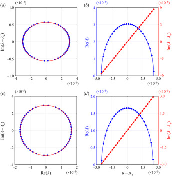
 ${O}(\varepsilon ^{2})$. In figure 6, we compare the ellipse with a subset of numerically computed eigenvalues on the
 $p=2$ isola for
 $\varepsilon = 0.01$ and find excellent agreement. We find similar agreement between the Floquet parameterization of the ellipse and of the numerically computed isola.
(a) The  $p=2$ isola with
 $\alpha = 1.5$ and
 $\varepsilon = 0.01$. The most unstable eigenvalue
 $\lambda _{*}$ is removed from the imaginary axis for better visibility. The solid red curve is the ellipse obtained by our asymptotic calculations. The blue dots are a subset of eigenvalues from the numerically computed isola using the FFH method. (b) The Floquet parameterization of the real (blue) and imaginary (red) parts of the isola on the left. The most unstable eigenvalue
 $\lambda _*$ and its corresponding Floquet exponent
 $\mu _*$ are removed from the imaginary and Floquet axes, respectively, for better visibility. The solid curves are our asymptotic results. The coloured dots are our numerical results using the FFH method. (c,d) Same with
 $\alpha = 1$.

The eigenvalue of largest real part on the ellipse occurs when  $\mu _2 = \mu _{2,*}$. Thus, the leading-order behaviour of the most unstable eigenvalue on the
 $p=2$ isola has real and imaginary parts
 \begin{gather} \lambda_{r,*} = \frac{\left|\mathcal{S}_2\right|}{2 \sqrt{\omega(n+\mu_0)\omega(n+p+\mu_0)}}\varepsilon^{2} + {O}\left(\varepsilon^{3}\right), \end{gather}
 \begin{gather}\lambda_{i,*} ={-}\varOmega_{1}\left(n+\mu_0\right) - \left(\frac{\mathfrak{p}_{2,n+p}c_{g,1}\left(n+\mu_0 \right)-\mathfrak{p}_{2,n}c_{g,-1}\left(n+p+\mu_0 \right)}{c_{g,-1}\left(n+p\!+\!\mu_0\right)-c_{g,1}\left(n+\mu_0\right)}\right)\varepsilon^{2} \!+\! {O}\left(\varepsilon^{3}\right), \end{gather}
respectively. The corresponding Floquet exponent is
 \begin{equation} \mu_* = \mu_0 + \mu_{2,*} \varepsilon^{2} +{O}\left(\varepsilon^{3}\right). \end{equation}
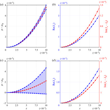
These expansions agree well with numerical results (figure 7).
Remark 5.2 According to figure 7,  $\mu _0$ is contained within the interval parameterizing the
 $p=2$ isola if the boundaries of this interval have opposite concavity at
 $\varepsilon =0$. This occurs if and only if
 $M_{2,+}M_{2,-}<0$. In figure 8, we plot
 $M_{2,+}M_{2,-}$ as a function of
 $\alpha$. We find
 $M_{2,+}M_{2,-}<0$ only if
 $\alpha \in (0.8643029367\dots, 1.0080416077\dots )$. Hur & Yang (Reference Hur and Yang2020) prove the existence of an eigenvalue with Floquet exponent
 $\mu _0$ on the
 $p=2$ isola for
 $\alpha$ in this interval. As we have demonstrated, to account for
 $p=2$ high-frequency instabilities that occur outside this interval, it is necessary to expand the Floquet exponent as a power series in
 $\varepsilon$ about
 $\mu _0$.
(a) The interval of Floquet exponents parameterizing the  $p=2$ isola as a function of
 $\varepsilon$ for
 $\alpha = 1.5$. The zeroth-order correction of the Floquet exponent is removed from the Floquet axis for better visibility. The solid blue curves are the boundaries of this interval according to our asymptotic calculations. The blue dots are the boundaries computed numerically by the FFH method. The solid red curve gives the Floquet exponent of the most unstable eigenvalue on the isola according to our asymptotic calculations. The red dots are the Floquet exponent of the most unstable eigenvalue as computed by the FFH method. (b) The real (blue) and imaginary (red) parts of the most unstable eigenvalue of the
 $p=2$ isola with
 $\alpha = 1.5$ as a function of
 $\varepsilon$. The zeroth-order correction of the eigenvalue is removed from the imaginary axis for better visibility. The solid curves are our asymptotic calculations. The coloured dots are our numerical results using the FFH method. (c,d) Same with
 $\alpha = 1$.

A plot of  $M_{2,+}M_{2,-}$ vs
 $\alpha$ (solid red). We find
 $M_{2,+}M_{2,-} < 0$ only when
 $\alpha \in (0.8643029367\dots, 1.0080416077\dots )$ (solid black). If
 $M_{2,+}M_{2,-} < 0$, the boundaries of the Floquet exponents parameterizing the
 $p=2$ isola have opposite concavities at
 $\varepsilon =0$. Only then does
 $\mu _0$ remain in the interval of Floquet exponents parameterizing the isola for positive
 $\varepsilon$.

5.3. The case of infinite depth
In infinite depth, the  $p=2$ isola originates from the eigenvalue
 \begin{equation} \lambda_0 ={-}\tfrac{3}{4}{\rm i}, \end{equation}
with corresponding Floquet exponent  $\mu _0 =-1/4$ and
 $n = -2$, see Remark 4.4. The corresponding eigenfunction, after normalizing, is
 \begin{equation} \boldsymbol{w}_0 = \begin{pmatrix} 1 \\ \frac 23 {\rm i} \end{pmatrix}{\rm e}^{{\rm i}nx} + \gamma_0 \begin{pmatrix} 1 \\ -2{\rm i} \end{pmatrix}{\rm e}^{{\rm i}(n+p)x}, \end{equation}
where  $\gamma _0 \in \mathbb {C} {\setminus} \{0 \}$. We modify the generalized eigenvalue problem (4.14) according to Remark 4.1 and expand the spectral data as a power series in
 $\varepsilon$ about the values above.
Terms of  ${O}(\varepsilon ^{0})$ cancel by construction. At
 ${O}(\varepsilon )$, the solvability conditions simplify to
 \begin{equation} \lambda_1 = 0 = \mu_1, \end{equation}
as in finite depth, and the normalized solution of the  ${O}(\varepsilon )$ problem is
 \begin{equation} \boldsymbol{w}_1 = \sum_{\substack{j = n-1 \\ j \neq n, n+p}}^{n+p+1} \hat{\mathcal{W}}_{1,j,\infty}{\rm e}^{{\rm i}jx} + \gamma_1 \begin{pmatrix} 1 \\ -2{\rm i}\end{pmatrix} {\rm e}^{{\rm i}(n+p)x}, \end{equation}
where the coefficients  $\hat {\mathcal {W}}_{1,j,\infty }$ depend at most linearly on
 $\gamma _0$.
At  ${O}(\varepsilon ^{2})$, the solvability conditions are
 \begin{gather} \lambda_2 + {\rm i}\mathfrak{c}_{2,1,n,\infty} = 0, \end{gather}
 \begin{gather}\gamma_0\left(\lambda_2 + {\rm i}\mathfrak{c}_{2,-1,n+p,\infty}\right) = 0, \end{gather}
where
 \begin{equation} \mathfrak{c}_{2,\sigma,j,\infty} = \mu_2 c_{g,\sigma,\infty}\left(j+\mu_0\right) - \mathfrak{p}_{2,j,\infty}, \end{equation}
with  $c_{g,\sigma,\infty }(z) = \lim _{\alpha \rightarrow \infty } \varOmega _{\sigma,z}(z)$,
 $\mathfrak {p}_{2,n,\infty } = 9/8$ and
 $\mathfrak {p}_{2,n+p,\infty } = -1/16$.
Because  $\gamma _0 \neq 0$, (5.26a)–(5.26b) reduce to a linear system for
 $\lambda _2$ and
 $\mu _2$. The solution of this system is
 \begin{equation} \lambda_2 = \tfrac{55}{32}{\rm i}, \quad \mu_2 = \tfrac{57}{64}. \end{equation}
Since  $\lambda _2$ is purely imaginary, the leading-order behaviour of the
 $p=2$ isola does not occur at
 ${O}(\varepsilon ^{2})$, as expected from (5.20a), since
 $\lim _{\alpha \rightarrow \infty }\mathcal {S}_2=0$. Thus, while the asymptotic expressions involved in infinite depth are simpler than those in finite depth, the leading-order behaviour of the
 $p=2$ isola requires a higher-order calculation in infinite depth. We obtain the normalized solution of the
 ${O}(\varepsilon ^{2})$ problem
 \begin{equation} \boldsymbol{w}_2 = \sum_{\substack{j = n-2}}^{n+p+2} \hat{\mathcal{W}}_{2,j,\infty}{\rm e}^{{\rm i}jx} + \gamma_2 \begin{pmatrix} 1 \\ -2{\rm i}\end{pmatrix} {\rm e}^{{\rm i}(n+p)x}, \end{equation}
where the coefficients  $\hat {\mathcal {W}}_{2,j,\infty }$ depend at most linearly on
 $\gamma _0$ and
 $\gamma _1$ while
 $\gamma _2 \in \mathbb {C}$ is a free parameter at this order.
At  ${O}(\varepsilon ^{3})$, the solvability conditions reduce to
 \begin{gather} \lambda_3 +{\rm i}\mu_3c_{g,1,\infty}\left(n+\mu_0\right) = 0, \end{gather}
 \begin{gather}\gamma_0\left( \lambda_3 + {\rm i} \mu_3c_{g,-1,\infty}\left(n+p+\mu_0\right)\right) = 0. \end{gather}
As in finite depth,  $c_{g,1,\infty }(n+\mu _0) \neq c_{g,-1,\infty }(n+p+\mu _0)$, and since
 $\gamma _0 \neq 0$, we must have
 \begin{equation} \lambda_3 = 0 = \mu_3. \end{equation}
No instability is observed at this order. The normalized solution of the  ${O}(\varepsilon ^{3})$ problem is
 \begin{equation} \boldsymbol{w}_3 = \sum_{\substack{j = n-3}}^{n+p+3} \hat{\mathcal{W}}_{3,j,\infty}{\rm e}^{{\rm i}jx} + \gamma_3 \begin{pmatrix} 1 \\ -2{\rm i}\end{pmatrix} {\rm e}^{{\rm i}(n+p)x}, \end{equation}
where the coefficients  $\hat {\mathcal {W}}_{3,j,\infty }$ depend at most linearly on
 $\gamma _0$,
 $\gamma _1$ and
 $\gamma _2$ while the parameter
 $\gamma _3 \in \mathbb {C}$ is free at this order.
At  ${O}(\varepsilon ^{4})$, the solvability conditions are
 \begin{gather} 2\left(\lambda_4 + {\rm i}\mathfrak{c}_{4,1,n,\infty}\right) + {\rm i}\gamma_0\mathfrak{s}_{4,n,\infty} = 0, \end{gather}
 \begin{gather}2\gamma_0\left(\lambda_4 + {\rm i}\mathfrak{c}_{4,-1,n+p,\infty}\right) + {\rm i} \mathfrak{s}_{4,n+p,\infty} = 0, \end{gather}
where
 \begin{equation} \mathfrak{c}_{4,\sigma,j,\infty} = \mu_4 c_{g,\sigma,\infty}\left({\rm j}+\mu_0\right) - \mathfrak{p}_{4,j,\infty}, \end{equation}
with  $\mathfrak {s}_{4,n,\infty } = -111/256$,
 $\mathfrak {s}_{4,n+p,\infty } = 37/256$,
 $\mathfrak {p}_{4,n,\infty } = 24\,119/12\,288$ and
 $\mathfrak {p}_{4,n+p,\infty } = 24\,985/36\,864$. Solving (5.33a)–(5.33b) for
 $\lambda _4$, we find the explicit formula
 \begin{equation} \lambda_4 = \frac{(48\,671+49152\mu_4)}{36\,864} {\rm i} \pm \frac{\sqrt{-134\,933\,977+291053568\mu_4-150994944\mu_4^{2}}}{18\,432}. \end{equation}
Equation (5.35) has non-zero real part provided
 \begin{equation} \mu_4 \in \left(\frac{11\,843}{12\,288} - \frac{111\sqrt{3}}{1024}, \frac{11\,843}{12\,288} + \frac{111\sqrt{3}}{1024} \right). \end{equation}
Thus, the  $p=2$ isola is an ellipse to
 ${O}(\varepsilon ^{4})$ given by the real and imaginary parts of
 \begin{equation} \lambda(\mu_4;\varepsilon) ={-}\tfrac 34 {\rm i} + \tfrac{55}{32}{\rm i}\varepsilon^{2} + \lambda_4(\mu_4)\varepsilon^{4}, \end{equation}
for  $\mu _4$ in (5.36). Unlike in finite depth, this ellipse has semi-major and -minor axes that are
 ${O}(\varepsilon ^{4})$, while the centre drifts from
 $\lambda _{0}$ like
 ${O}(\varepsilon ^{2})$. Similarly, the Floquet parameterization of the isola has width
 ${O}(\varepsilon ^{4})$ and drifts from
 $\mu _0$ like
 ${O}(\varepsilon ^{2})$.
In figure 9, we compare the asymptotically computed ellipse with a subset of numerically computed eigenvalues on the  $p=2$ isola for
 $\varepsilon = 0.01$. Notice this ellipse is considerably smaller than that in finite depth for comparable wave amplitude (figure 6). Excellent agreement is found between the asymptotic and numerical predictions. Similar agreement is found between the Floquet parameterization of the ellipse and of the numerically computed isola.
(a) The  $p=2$ isola with
 $\alpha =\infty$ and
 $\varepsilon = 0.01$. The most unstable eigenvalue
 $\lambda _{*}$ is removed from the imaginary axis for better visibility. The solid red curve is the ellipse obtained by our asymptotic calculations. The blue dots are a subset of eigenvalues from the numerically computed isola using the FFH method. (b) The Floquet parameterization of the real (blue) and imaginary (red) parts of the isola. The most unstable eigenvalue
 $\lambda _*$ and its corresponding Floquet exponent
 $\mu _*$ are removed from the imaginary and Floquet axes, respectively, for better visibility. The solid curves are our asymptotic results. The coloured dots are our numerical results using the FFH method.

The eigenvalue of largest real part on the ellipse occurs when  $\mu _4 = 11843/36864$. Thus, the real and imaginary parts of the most unstable eigenvalue on the isola have asymptotic expansions
 \begin{gather} \lambda_{r,*} = \frac{37\sqrt{3}}{512} \varepsilon^{4} + {O}\left(\varepsilon^{5}\right), \end{gather}
 \begin{gather}\lambda_{i,*} ={-}\frac 34 + \frac{55}{32} \varepsilon^{2} + \frac{96\,043}{36\,864} \varepsilon^{4} + {O}\left(\varepsilon^{5}\right), \end{gather}
respectively. The corresponding Floquet exponent has expansion
 \begin{equation} \mu_* ={-}\frac 14 + \frac{57}{64}\varepsilon^{2} + \frac{11\,843}{36\,864}\varepsilon^{4} + {O}\left(\varepsilon^{5}\right). \end{equation}
These expansions are compared with numerical results in figure 10.
(a) The interval of Floquet exponents parameterizing the  $p=2$ isola as a function of
 $\varepsilon$ for
 $\alpha = \infty$. The most unstable Floquet exponent
 $\mu _*$ is removed from the Floquet axis for better visibility. The solid blue curves are the boundaries of this interval according to our asymptotic calculations. The blue dots are the boundaries computed numerically by the FFH method. The solid red curve gives the Floquet exponent of the most unstable eigenvalue on the isola according to our asymptotic calculations. The red dots are the Floquet exponent of the most unstable eigenvalue as computed by the FFH method. (b) The real (blue) and imaginary (red) parts of the most unstable eigenvalue of the
 $p=2$ isola with
 $\alpha = \infty$ as a function of
 $\varepsilon$. The zeroth-order correction of the eigenvalue is removed from the imaginary axis for better visibility. The solid curves are our asymptotic calculations. The coloured dots are our numerical results using the FFH method.

6. Second isola. High-frequency instabilities: $p=3$

We extend the perturbation method developed in § 5 to obtain the leading-order behaviour of the high-frequency isola that arises from  $\lambda _{0,p}$ with
 $p=3$. This isola is the second closest to the origin by Theorem 1, and its leading-order behaviour is obtained at
 ${O}(\varepsilon ^{3})$.
As in the previous section, we expand the spectral data of (4.14) according to (5.1a)–(5.1c) and normalize the eigenfunctions according to (5.2) for convenience. The perturbation method proceeds as in § 5, with two major changes:
(i) At
${O}(\varepsilon ^{2})$, the solvability conditions are independent of $\gamma _0$ and linear in $\lambda _2$ and $\mu _2$. As a consequence, $\lambda _2$ is purely imaginary, and the leading-order behaviour of the isola is undetermined at this order.(ii) At
${O}(\varepsilon ^{3})$, the solvability conditions depend on $\gamma _0$, $\lambda _3$, and $\gamma _1$. Using solvability conditions from the previous order together with the collision condition (4.21), one shows that the dependence on $\gamma _1$ vanishes from these conditions.


A more complete description of these calculations is provided in Appendix B.
6.1. The ${O}(\varepsilon ^{3})$ problem

Solving for  $\lambda _3$ in the solvability conditions at
 ${O}(\varepsilon ^{3})$, we find
 \begin{align} \lambda_3 &={-}{\rm i}\mu_3\left(\frac{c_{g,-1}(n+p+\mu_0) + c_{g,1}(n+\mu_0)}{2} \right) \nonumber\\ &\quad \pm \sqrt{-\mu_3^{2}\left(\frac{c_{g,-1}(n+p+\mu_0) -c_{g,1}(n+\mu_0)}{2} \right)^{2} + \frac{\mathcal{S}_3^{2}}{4\omega(n+\mu_0)\omega(n+p+\mu_0)} }. \end{align}
Similar to  $\mathcal {S}_2$ in the previous section,
 $\mathcal {S}_3$ is another lengthy expression depending only on
 $\alpha$, see Appendix B for more details. A plot of
 $\mathcal {S}_3$ vs
 $\alpha$ reveals
 $\mathcal {S}_3 \neq 0$, except at
 $\alpha _2 = 0.8206431673\dots$ (figure 11). We conjecture that Stokes waves of all wavenumbers and in all depths are unstable to the second closest high-frequency instability from the origin, with possible exceptions if
 $\alpha = \alpha _2$. Since
 $\alpha _2\neq \alpha _1$, Stokes waves of all wavenumbers and in all depths appear to be unstable with respect to high-frequency instabilities.
Remark 6.1 As  $\alpha \rightarrow \infty$,
 $\mathcal {S}_3 \rightarrow 0$. Therefore, the leading-order behaviour of the
 $p=3$ isola in infinite depth is resolved at higher order. For
 $\varepsilon$ of the order of 0.01 and smaller, this isola is already within the numerical error of the FFH method. For larger
 $\varepsilon$, the expansions deviate too quickly from the numerics to make comparisons.
(a) A plot of  $\mathcal {S}_3$ vs
 $\alpha$ (solid red). The zero of
 $\mathcal {S}_3$ for
 $\alpha > 0$ is
 $\alpha _2 = 0.8206431673\dots$ (gold star). (b) The real part
 $\lambda _{r,*}$ of the most unstable eigenvalue on the
 $p=3$ isola as a function of
 $\alpha$ according to our asymptotic calculations (solid red). The real part of the eigenvalue is normalized by
 $\varepsilon ^{3}$ for better visibility. We zoom-in around
 $\alpha = \alpha _2$ (gold star) in the inlay. The real part of the most unstable eigenvalue on the isola vanishes as
 $\alpha \rightarrow \alpha _2$ according to our asymptotic calculations, which agrees with our numerical results using the FFH method with
 $\varepsilon = 0.01$ (blue dots).

Provided  $\alpha \neq \alpha _2$, (6.1) has non-zero real part for
 $\mu _3 \in (-M_3,M_3)$, where
 \begin{equation} M_3 = \frac{|\mathcal{S}_3|}{|c_{g,-1}(n+p+\mu_0) - c_{g,1}(n+\mu_0)|\sqrt{\omega(n+\mu_0)\omega(n+p+\mu_0)}}. \end{equation}
Unlike the  $p=2$ isola, this interval is symmetric about the origin. For
 $\mu _3$ in this interval, the real and imaginary parts of (6.1), together with the lower-order corrections of
 $\lambda$, trace an ellipse asymptotic to the
 $p=3$ isola. This ellipse has semi-major and -minor axes that scale as
 ${O}(\varepsilon ^{3})$ and a centre that drifts form
 $\lambda _0$ like
 ${O}(\varepsilon ^{2})$. The Floquet parameterization of this ellipse has width
 ${O}(\varepsilon ^{3})$ and drifts from
 $\mu _0$ like
 ${O}(\varepsilon ^{2})$. As a result, this isola is more challenging to capture than the
 $p=2$ isola in finite depth.
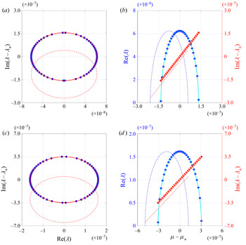
Comparing our asymptotic and numerical  $p=3$ isolas with
 $\varepsilon = 0.01$ (figure 12), we observe that, while the real part of the numerical isola matches our
 ${O}(\varepsilon ^{3})$ calculations, the imaginary part and Floquet parameterization of the isola require fourth-order corrections. This is in contrast with the
 $p=2$ isola (figure 6), for which we obtain the drifts in the imaginary part and Floquet parameterization at the same order as the real part. We obtain these drifts for the
 $p=3$ isola in the following subsection.
(a) The  $p=3$ isola with
 $\alpha = 1.5$ and
 $\varepsilon = 0.01$. The most unstable eigenvalue
 $\lambda _{*}$ is removed from the imaginary axis for better visibility. The solid and dashed red curves are the ellipses obtained by our
 ${O}(\varepsilon ^{4})$ and
 ${O}(\varepsilon ^{3})$ asymptotic calculations, respectively. The blue dots are a subset of eigenvalues from the numerically computed isola using the FFH method. (b) The Floquet parameterization of the real (blue) and imaginary (red) parts of the isola on the left. The most unstable eigenvalue
 $\lambda _*$ and its corresponding Floquet exponent
 $\mu _*$ are removed from the imaginary and Floquet axes, respectively, for better visibility. The solid teal and orange curves are our asymptotic results for the real and imaginary parts of the Floquet parameterization, respectively, to
 ${O}(\varepsilon ^{4})$. The dashed blue and red curves are the same results to
 ${O}(\varepsilon ^{3})$. The blue and red dots are the numerically computed real and imaginary parts of the Floquet parameterization, respectively, using the FFH method. (c,d) Same with
 $\alpha = 1$.

Equating  $\mu _3 = 0$ maximizes the real part of (6.1). Hence, the real and imaginary part of the most unstable eigenvalue on the
 $p=3$ isola have asymptotic expansions
 \begin{gather} \lambda_{r,*} = \left( \frac{|\mathcal{S}_3|}{2\sqrt{\omega(n+\mu_0)\omega(n+p+\mu_0)}}\right)\varepsilon^{3} + {O}\left(\varepsilon^{4}\right), \end{gather}
 \begin{gather}\lambda_{i,*} ={-}{\rm i}\varOmega_1(n+\mu_0) -\left(\frac{\mathfrak{p}_{2,n+p}c_{g,1}(n+\mu_0) - \mathfrak{p}_{2,n}c_{g,-1}(n+p+\mu_0)}{c_{g,-1}(n+p+\mu_0)-c_{g,1}(n+\mu_0)}\right)\varepsilon^{2} +{O}\left(\varepsilon^{4}\right), \end{gather}
respectively, and the corresponding Floquet exponent has asymptotic expansion
 \begin{equation} \mu_* = \mu_0 + \left(\frac{\mathfrak{p}_{2,n+p}-\mathfrak{p}_{2,n}}{c_{g,-1}(n+p+\mu_0)-c_{g,1}(n+\mu_0)}\right)\varepsilon^{2} + {O}\left(\varepsilon^{4}\right). \end{equation}
The quantities  $\mathfrak {p}_{2,j}$ are defined in Appendix B.
Figure 13 compares the asymptotic expansions (6.3a)–(6.3b) and (6.4) with their numerical counterparts. Excellent agreement is found for the real and imaginary parts of the most unstable eigenvalue. The interval of Floquet exponents that parameterizes the isola requires a fourth-order correction to match the numerical predictions.
(a) The interval of Floquet exponents parameterizing the  $p=3$ isola as a function of
 $\varepsilon$ for
 $\alpha = 1.5$. The most unstable Floquet exponent
 $\mu _*$ is removed from the Floquet axis for better visibility. The solid and dashed blue curves are the boundaries of this interval according to our
 ${O}(\varepsilon ^{4})$ and
 ${O}(\varepsilon ^{3})$ asymptotic calculations, respectively. The blue dots are the boundaries computed numerically by the FFH method. The solid and dashed red curves give the Floquet exponent of the most unstable eigenvalue on the isola according to our
 ${O}(\varepsilon ^{4})$ and
 ${O}(\varepsilon ^{3})$ asymptotic calculations, respectively. The red dots are the Floquet exponent of the most unstable eigenvalue as computed by the FFH method. (b) The real (blue) and imaginary (red) parts of the most unstable eigenvalue of the
 $p=3$ isola with
 $\alpha = 1.5$ as a function of
 $\varepsilon$. The zeroth-order correction of the eigenvalue is removed from the imaginary axis for better visibility. The solid teal and orange curves are our asymptotic calculations for the real and imaginary parts of the most unstable eigenvalue to
 ${O}(\varepsilon ^{4})$, respectively. The dashed blue and red curves are the same results to
 ${O}(\varepsilon ^{3})$. The blue and red dots are the numerically computed real and imaginary parts of the most unstable eigenvalue using the FFH method. (c,d) Same with
 $\alpha = 1$.

Before proceeding to the next order, we solve the  ${O}(\varepsilon ^{3})$ problem for
 $\boldsymbol {w}_3$:
 \begin{equation} \boldsymbol{w}_3 = \sum_{\substack{j = n-3} }^{n+p+3} \hat{\mathcal{W}}_{3,j} {\rm e}^{{\rm i}jx} + \gamma_3 \begin{pmatrix} 1 \\ \dfrac{{\rm i}}{\omega(n+p+\mu_0)} \end{pmatrix} {\rm e}^{{\rm i}(n+p)x}, \end{equation}
where the coefficients  $\hat {\mathcal {W}}_{3,j}$ depend on
 $\alpha$ (possibly through intermediate dependencies on known zeroth-, first- and second-order results) and at most linearly on
 $\gamma _0, \gamma _1,$ and
 $\gamma _2$. At this order,
 $\gamma _3 \in \mathbb {C}$ is a free parameter.
6.2. The ${O}(\varepsilon ^{4})$ problem

At  ${O}(\varepsilon ^{4})$, the spectral problem (4.14) becomes
 \begin{align} \left(L_0 - \lambda_0R_0 \right)\boldsymbol{w}_4 &= \left(\sum_{j=0}^{2}\lambda_{4-j} R_j\right)\boldsymbol{w}_0 + \left( \sum_{j=0}^{1} \lambda_{3-j} R_j \right)\boldsymbol{w}_1 + \lambda_2R_0\boldsymbol{w}_2 \nonumber\\ &\quad - \sum_{j=0}^{3}\left(L_{4-j}-\lambda_0R_{4-j} \right)\boldsymbol{w}_j. \end{align}
After some manipulation, the solvability conditions of (6.6) can be written as
 \begin{align} & \begin{pmatrix} 2 & {\rm i}\mathfrak{s}_{3,n} \\ 2\gamma_0 & 2\left(\lambda_3 +{\rm i}\mu_3c_{g,-1}(n+p+\mu_0) \right) \end{pmatrix} \begin{pmatrix} \lambda_4 \\ \gamma_1 \end{pmatrix} + {\rm i}\gamma_2 \begin{pmatrix} 0 \\ \mathfrak{t}_{4,n+p}\end{pmatrix} \nonumber\\ &\quad ={-}2{\rm i}\begin{pmatrix} \mu_4c_{g,1}(n+\mu_0)-\mathfrak{p}_{4,n} \\ \gamma_0\left(\mu_4c_{g,-1}(n+p+\mu_0) - \mathfrak{p}_{4,n+p} \right) \end{pmatrix}. \end{align}
Using the solvability conditions at the previous order and the collision condition (4.21), one can show  $\mathfrak {t}_{4,n+p} \equiv 0$. Then, (6.7) reduces to a linear system for
 $\lambda _4$ and
 $\gamma _1$.
For  $\mu _3 \in (-M_3,M_3)$ with
 $M_3$ given by (6.2), the determinant of (6.7) simplifies to
 \begin{equation} \textrm{det}\begin{pmatrix} 2 & {\rm i}\mathfrak{s}_{3,n} \\ 2\gamma_0 & 2\left(\lambda_3 +{\rm i}\mu_3c_{g,-1}(n+p+\mu_0) \right) \end{pmatrix} = 8\lambda_{3,r}, \end{equation}
where  $\lambda _{3,r} = \textrm {Re}(\lambda _3).$ Provided
 $\alpha \neq \alpha _2$, (6.7) is invertible for all
 $\mu _3 \in (-M_3,M_3)$.
Solving (6.7) for  $\lambda _4$,
 \begin{align} \lambda_4 & ={\rm i}\left[\frac{\left(\lambda_3 + {\rm i}\mu_3c_{g,-1}(n+p+\mu_0) \right) \left(c_{g,1}(n+\mu_0)-\mathfrak{p}_{4,n} \right)}{2\lambda_{3,r}} \right.\nonumber\\ &\quad \left. + \frac{\left(\lambda_3 + {\rm i}\mu_3c_{g,1}(n+\mu_0) \right)\left(c_{g,-1}(n+p+\mu_0)-\mathfrak{p}_{4,n+p} \right)}{2\lambda_{3,r}} \right]. \end{align}
Since  $\mathfrak {p}_{4,j}, \mu _4 \in \mathbb {R}$, the real and imaginary parts of
 $\lambda _4=\lambda _{4,r}+i \lambda _{4,i}$ are
 \begin{align} \lambda_{4,r} &= \frac{\mu_3\left(c_{g,-1}(n+p+\mu_0)-c_{g,1}(n+\mu_0) \right)}{4\lambda_{3,r}}\left[ -\mu_4\left(c_{g,-1}(n+p+\mu_0) - c_{g,1}(n+\mu_0)\right)\right.\nonumber\\ &\quad + \left.\mathfrak{p}_{2,n+p} - \mathfrak{p}_{2,n} \right], \end{align}
 \begin{equation} \lambda_{4,i} ={-}\tfrac{1}{2}\big[\mu_4\left(c_{g,-1}(n+\mu_0) + c_{g,1}(n+\mu_0)\right) - \left(\mathfrak{p}_{4,n+p} + \mathfrak{p}_{4,n} \right) \big]. \end{equation}
Given (6.10a)–(6.10b), we invoke the regular curve condition, first introduced in Creedon et al. (Reference Creedon, Deconinck and Trichtchenko2021a,Reference Creedon, Deconinck and Trichtchenkob). According to this condition, all eigenvalue corrections must be bounded over the closure of  $\mu _3 \in (-M_3,M_3)$. Notice
 $\lambda _{3,r} \rightarrow 0$ as
 $|\mu _3| \rightarrow M_3$. Thus,
 $\lambda _{4,r}$ is bounded only if
 \begin{equation} \mu_4 = \frac{\mathfrak{p}_{4,n+p}-\mathfrak{p}_{4,n}}{c_{g,-1}(n+p+\mu_0)-c_{g,1}(n+\mu_0)}. \end{equation}
Hence,
 \begin{equation} \lambda_4 ={-}{\rm i}\left(\frac{\mathfrak{p}_{4,n+p}c_{g,1}(n+\mu_0) - \mathfrak{p}_{4,n}c_{g,-1}(n+p+\mu_0)}{c_{g,-1}(n+p+\mu_0)-c_{g,1}(n+\mu_0)}\right). \end{equation}
Remark 6.2 If  $\alpha = \alpha _2$, then
 $\mathfrak {s}_{3,n} =0$ and
 $\lambda _3 = 0 = \mu _3$. Applying the Fredholm alternative to (6.7), one arrives at (6.11) and (6.12), but the constants
 $\gamma _0$ and
 $\gamma _1$ remain arbitrary at this order.
Equations (6.11) and (6.12) give the fourth-order drifts in the Floquet parameterization and imaginary part of the  $p=3$ isola, respectively. The eigenvalues asymptotic to this isola form the ellipse
 \begin{equation} \lambda(\mu_3;\varepsilon) = \lambda_0 + \lambda_2\varepsilon^{2} + \lambda_3(\mu_3)\varepsilon^{3} + \lambda_4 \varepsilon^{4}, \end{equation}
which agrees better with the numerically computed isola than at the previous order, see figures 12 and 13.
7. Conclusion
Building on previous work by Akers (Reference Akers2015) and Creedon et al. (Reference Creedon, Deconinck and Trichtchenko2021a,Reference Creedon, Deconinck and Trichtchenkob), we have developed a formal perturbation method to compute high-frequency instabilities of small-amplitude Stokes wave solutions of Euler's equations in arbitrary depth. This method allows one to approximate an entire high-frequency isola.
We explicitly obtain the leading-order behaviour of the isolas closest to the origin in the complex spectral plane ( $p=2,3$) for all depths, including
(i) the Floquet exponents that parameterize the isola;
(ii) the real and imaginary parts of the most unstable eigenvalue on the isola; and
(iii) the curve asymptotic to the isola.
These expressions are compared directly with numerical computations of the isolas using the FFH method. Excellent agreement is found for the  $p=2$ isola. The
 $p=3$ isola achieves similar agreement if higher-order corrections of the imaginary part and Floquet parameterization are computed using the regular curve condition, as defined in § 6.
According to our asymptotic results, Stokes waves of all aspect ratios, except  $\kappa h = \alpha _1$ and
 $\kappa h = \alpha _2$, are unstable to the
 $p=2$ and
 $p=3$ high-frequency instabilities, respectively. Stokes waves are also unstable to high-frequency instabilities in infinite depth (
 $h=\infty$), although this requires a higher-order calculation than in finite depth. Based on these findings, we conjecture that Stokes waves of all depths and all wavenumbers are spectrally unstable to high-frequency instabilities, extending recent work by Hur & Yang (Reference Hur and Yang2020), where the existence of the
 $p=2$ high-frequency instability is proven only if
 $\kappa h \in (0.86430\dots,1.00804\dots )$. The effect of the high-frequency instabilities on the Stokes waves has been illustrated in Deconinck & Oliveras (Reference Deconinck and Oliveras2011).
The perturbation method developed in this work is readily extended to higher-order isolas  $(p \geq 4)$. It appears this method yields the first real-part correction of the isola at
 ${O}(\varepsilon ^{p})$. In contrast, corrections to the imaginary part and Floquet parameterization of the isola appear at
 ${O}(\varepsilon ^{2})$. Thus, we expect isolas further from the origin to have increasingly smaller widths, while their centres drift along the imaginary axis like
 ${O}(\varepsilon ^{2})$.
If correct, this conjecture highlights one of the primary challenges for analytical and numerical investigations of high-frequency instabilities: each isola is smaller than the previous, and each isola drifts from its known zeroth-order behaviour quickly relative to its size. Our hope is that the perturbation method developed in this work can be used as a starting point for future proofs of high-frequency instabilities as well as improvements to the numerical resolution of high-frequency isolas far away from the origin in the complex spectral plane.
Acknowledgements
This paper is dedicated to Harvey Segur, on the occasion of his 80th birthday.
Funding
R.C. gratefully acknowledges funding from an ARCS Foundation Fellowship and from the Ruth Jung Chinn Fellowship in Applied Mathematics at the University of Washington.
Declaration of interests
The authors report no conflict of interest.
Data availability statement
The asymptotic expressions derived in this work can be found in the following Mathematica notebooks: wwp_isola_p2.nb ( $p=2$ isola in finite depth), wwp_isola_p2_id.nb (
 $p=2$ isola in infinite depth) and wwp_isola_p3.nb (
 $p=3$ isola in finite depth).
Appendix A. Stokes wave expansions
The Stokes waves of (2.3a)–(2.3b) have velocity
 \begin{equation} c(\varepsilon) = c_0 + c_2\varepsilon^{2} + c_4\varepsilon^{4} + {O}\left(\varepsilon^{6}\right), \end{equation}
where
 \begin{gather} c_0^{2} = \tanh(\alpha), \end{gather}
 \begin{gather}c_2 = \frac{6+2\cosh(2\alpha)+\cosh(4\alpha)}{16c_0\sinh^{3}(\alpha)\cosh(\alpha)}, \end{gather}
 \begin{gather}c_4 = \frac{212 + 55\cosh(2\alpha)-98\cosh(4\alpha)-23\cosh(6\alpha)+14\cosh(8\alpha)+2\cosh(10\alpha)}{2048c_0\sinh^{9}(\alpha)\cosh(\alpha)}, \end{gather}
and take the form
 \begin{align} \eta_S(x;\varepsilon) &= \varepsilon \cos(x) \!+\! \varepsilon^{2}\hat{N}_{2,2}\cos(2x) \!+\! \varepsilon^{3}\hat{N}_{3,3}\cos(3x) + \varepsilon^{4}\left(\hat{N}_{4,2}\cos(2x) + \hat{N}_{4,4}\cos(4x) \right)\nonumber\\ &\quad + {O}\left(\varepsilon^{5}\right), \end{align}
 \begin{align} q_{S,x}(x;\varepsilon) &= \frac{\varepsilon}{c_0}\cos(x) + \varepsilon^{2}\left(\hat{Q}_{2,0} + \hat{Q}_{2,2}\cos(2x) \right) + \varepsilon^{3} \left(\hat{Q}_{3,0}\cos(x) + \hat{Q}_{3,3}\cos(3x)\right) \nonumber\\ &\quad + \varepsilon^{4}\left(\hat{Q}_{4,0} + \hat{Q}_{4,2}\cos(2x) + \hat{Q}_{4,4}\cos(4x) \right) + {O}\left(\varepsilon^{5}\right), \end{align}
where
 \begin{gather} \hat{N}_{2,2} = \frac{5\cosh(\alpha)+\cosh(3\alpha)}{8\sinh^{3}(\alpha)}, \end{gather}
 \begin{gather}\hat{N}_{3,3} = \frac{3(14+15\cosh(2\alpha)+6\cosh(4\alpha)+\cosh(6\alpha))}{256\sinh^{6}(\alpha)}, \end{gather}
 \begin{gather}\hat{N}_{4,2} = \frac{215-418\cosh(2\alpha)-472\cosh(4\alpha)+10\cosh(6\alpha)+17\cosh(8\alpha)}{3072c_0^{2}\sinh^{8}(\alpha)}, \end{gather}
 \begin{gather}\hat{N}_{4,4} = \frac{203+347\cosh(2\alpha)+158\cosh(4\alpha) + 76\cosh(6\alpha)+23\cosh(8\alpha)+3\cosh(10\alpha)}{768c_0^{2}(2+3\cosh(2\alpha))\sinh^{8}(\alpha)}, \end{gather}
 \begin{gather}\hat{Q}_{2,0} = \frac{1}{4\sinh^{2}(\alpha)}, \end{gather}
 \begin{gather}\hat{Q}_{2,2} = \frac{3+2\cosh(2\alpha)+\cosh(4\alpha)}{8c_0\sinh^{3}(\alpha)\cosh(\alpha)}, \end{gather}
 \begin{gather}\hat{Q}_{3,1} ={-}\left(\frac{\cosh(2\alpha)\left(2 + \cosh(2\alpha)\right)}{16c_0\sinh^{4}(\alpha)} \right), \end{gather}
 \begin{gather}\hat{Q}_{3,3} = \frac{3\left(26 - 3\cosh(2\alpha)+10\cosh(4\alpha)+3\cosh(6\alpha) \right)}{256c_0\sinh^{6}(\alpha)}, \end{gather}
 \begin{gather}\hat{Q}_{4,0} = \frac{48+47\cosh(2\alpha)-20\cosh(4\alpha)-3\cosh(6\alpha)}{512c_0\sinh^{7}(\alpha)\cosh(\alpha)}, \end{gather}
 \begin{gather}\hat{Q}_{4,2} ={-}\left(\frac{240+82\cosh(2\alpha)+688\cosh(4\alpha)+309\cosh(6\alpha) - 16\cosh(8\alpha) - 7\cosh(10\alpha)}{6144c_0\sinh^{9}(\alpha)\cosh(\alpha)} \right), \end{gather}
 \begin{gather}\hat{Q}_{4,4} = \frac{408\!+\!638\cosh(2\alpha)\!+\!230\cosh(4\alpha) \!+\! 171\cosh(6\alpha) \!+\! 124\cosh(8\alpha)+43\cosh(10\alpha) + 6\cosh(12\alpha)}{1536c_0(2+3\cosh(2\alpha))\sinh^{9}(\alpha)\cosh(\alpha)}. \end{gather}
The Stokes expansions in infinite depth are obtained from the above with  $\alpha \rightarrow \infty$.
Appendix B. Detailed calculations of the $p=3$ instability

For explicit representations of the asymptotic expressions derived in this appendix, see the Data Availability Statement at the end of this manuscript.
B.1. The ${O}(\varepsilon )$ problem

At  ${O}(\varepsilon )$, the spectral problem takes the form (5.3). The solvability conditions simplify to
 \begin{equation} \lambda_1 = 0 = \mu_1, \end{equation}
and the normalized solution of the  ${O}(\varepsilon )$ problem is
 \begin{equation} \boldsymbol{w}_1 = \sum_{\substack{j = n-1 \\ j \neq n, n+p}}^{n+p+1} \hat{\mathcal{W}}_{1,j} {\rm e}^{{\rm i}jx} + \gamma_1 \begin{pmatrix} 1 \\ \dfrac{{\rm i}}{\omega(n+p+\mu_0)} \end{pmatrix} {\rm e}^{{\rm i}(n+p)x}, \end{equation}
where the coefficients  $\hat {\mathcal {W}}_{1,j}$ depend on
 $\alpha$ (possibly through intermediate dependencies on known zeroth-order results) and at most linearly on
 $\gamma _0$. At this order,
 $\gamma _1 \in \mathbb {C}$ is a free parameter.
B.2. The ${O}(\varepsilon ^{2})$ problem

At  ${O}(\varepsilon ^{2})$, the spectral problem takes the form (5.11). The solvability conditions are
 \begin{gather} \lambda_2 + {\rm i}\mathfrak{c}_{2,1,n} = 0, \end{gather}
 \begin{gather}\gamma_0\left(\lambda_2 + {\rm i}\mathfrak{c}_{2,-1,n+p}\right) = 0, \end{gather}
where  $\mathfrak {c}_{2,\sigma,j} = \mu _2 c_{g,\sigma }(j+\mu _0) - \mathfrak {p}_{2,j}$, as in § 5 (although the quantities
 $\mathfrak {p}_{2,j}$ evaluate differently than those for the
 $p=2$ isolas). Since
 $\gamma _0 \neq 0$, the solution of (B3a)–(B3b) is
 \begin{gather} \lambda_2 ={-}{\rm i}\left(\frac{\mathfrak{p}_{2,n+p}c_{g,1}(n+\mu_0) - \mathfrak{p}_{2,n} c_{g,-1}(n+p+\mu_0)}{c_{g,-1}(n+p+\mu_0)-c_{g,1}(n+\mu_0)}\right), \end{gather}
 \begin{gather}\mu_2 = \frac{\mathfrak{p}_{2,n+p}-\mathfrak{p}_{2,n}}{c_{g,-1}(n+p+\mu_0)-c_{g,1}(n+\mu_0)}. \end{gather}
Since  $\lambda _2$ is purely imaginary, no instabilities are found at this order. The normalized solution of the
 ${O}(\varepsilon ^{2})$ problem is
 \begin{equation} \boldsymbol{w}_2 = \sum_{\substack{j = n-2} }^{n+p+2} \hat{\mathcal{W}}_{2,j} {\rm e}^{{\rm i}jx} + \gamma_2 \begin{pmatrix} 1 \\ \dfrac{{\rm i}}{\omega(n+p+\mu_0)} \end{pmatrix} {\rm e}^{{\rm i}(n+p)x}, \end{equation}
where the coefficients  $\hat {\mathcal {W}}_{2,j}$ depend on
 $\alpha$ (possibly through intermediate dependencies on known zeroth- and first-order results) and at most linearly on
 $\gamma _0$ and
 $\gamma _1$. At this order,
 $\gamma _2 \in \mathbb {C}$ is a free parameter.
B.3. The ${O}(\varepsilon ^{3})$ problem

At  ${O}(\varepsilon ^{3})$, the spectral problem becomes
 \begin{equation} \left(L_0-\lambda_0R_0 \right)\boldsymbol{w}_3 = \left(\lambda_2 R_1 + \lambda_3 R_0\right)\boldsymbol{w}_0 - \sum_{j=0}^{2}\left(L_{3-j} -\lambda_0R_{3-j} \right)\boldsymbol{w}_j, \end{equation}
with the aid of (B1). The solvability conditions are
 \begin{gather} 2\left(\lambda_3 + {\rm i}\mu_3c_{g,1}(n+\mu_0)\right) + {\rm i}\gamma_0\mathfrak{s}_{3,n} = 0, \end{gather}
 \begin{gather}2\gamma_0\left(\lambda_3 + {\rm i}\mu_3c_{g,-1}(n+p+\mu_0)\right) + {\rm i} \mathfrak{s}_{3,n+p} + {\rm i}\gamma_1 \mathfrak{t}_{3,n+p}= 0. \end{gather}
Using the solvability conditions (B3a)–(B3b) and the collision condition (4.21), it can be shown that
 \begin{equation} \mathfrak{t}_{3,n+p} \equiv 0. \end{equation}
As in the  $p=2$ case (§ 5), the product of
 $\mathfrak {s}_{3,n}$ and
 $\mathfrak {s}_{3,n+p}$ is related to a perfect square
 \begin{equation} \mathfrak{s}_{3,n}\mathfrak{s}_{3,n+p} ={-}\frac{\mathcal{S}_3^{2}}{\omega(n+\mu_0)\omega(n+p+\mu)}, \end{equation}
where
 \begin{equation} \mathcal{S}_3 = \mathcal{T}_{3,1} + \mathcal{T}_{3,2}\hat{N}_{2,2} + \mathcal{T}_{3,3}\hat{Q}_{2,2} + \mathcal{T}_{3,4}\hat{N}_{3,3} + \mathcal{T}_{3,5}\hat{Q}_{3,3}. \end{equation}
The expressions  $\mathcal {T}_{3,j}$ are functions only of
 $\alpha$, as are the Stokes wave corrections
 $\hat {N}_{2,2}$,
 $\hat {Q}_{2,2}$,
 $\hat {N}_{3,3}$ and
 $\hat {Q}_{3,3}$, see Appendix A. When fully expanded,
 $\mathcal {S}_3$ involves several hundred terms, but each term depends only on
 $\alpha$. The full expression of
 $\mathcal {S}_3$ can be found in the appropriate Mathematica notebook provided in the Data Availability Statement. The remaining calculations at this order appear in § 6.