2 Theoretical development

Consider a two-dimensional porous medium of uniform permeability $k$ and porosity ${\it\phi}$ saturated by fluid of constant viscosity ${\it\mu}$ but variable density ${\it\rho}(\boldsymbol{x},t)$ , where $\boldsymbol{x}\equiv (x,z)$ , as illustrated in figure 1. We assume a constant reference pressure $p_{\infty }$ along the horizontal line $z=\mathscr{H}$ , equivalent to assuming that the medium is much deeper than the vertical scales of the flow. The fluid flow is modelled as incompressible and governed by Darcy’s law, with momentum and mass continuity equations given by

(2.1a,b ) $$\begin{eqnarray}\displaystyle {\it\mu}{\it\phi}\boldsymbol{u}=k(-\boldsymbol{{\rm\nabla}}p-{\it\rho}g\hat{\boldsymbol{z}})\quad \text{and}\quad \boldsymbol{{\rm\nabla}}\boldsymbol{\cdot }\boldsymbol{u}=0, & & \displaystyle\end{eqnarray}$$

respectively, where $\boldsymbol{u}(\boldsymbol{x},t)\equiv (u,w)$ is the interstitial (pore) velocity, $p(\boldsymbol{x},t)$ is the fluid pressure and $\boldsymbol{{\rm\nabla}}$ is the gradient operator (Bear Reference Bear1988). For incompressible fluids, density is materially conserved and is thus governed by the advection equation

(2.2) $$\begin{eqnarray}\frac{\text{D}{\it\rho}}{\text{D}t}\equiv \frac{\partial {\it\rho}}{\partial t}+\boldsymbol{u}\boldsymbol{\cdot }\boldsymbol{{\rm\nabla}}{\it\rho}=0.\end{eqnarray}$$

Thermal and solutal diffusivity are neglected. In writing (2.2), we also assume that there are no capillary forces acting between the fluids, which could otherwise control the density field through a capillary fringe (Golding et al. Reference Golding, Neufeld, Hesse and Huppert2011). Under our assumption of a deep porous medium ( $h\ll \mathscr{H}$ ), the results of this paper are equally applicable to situations with a confining or free upper boundary (Hesse et al. Reference Hesse, Tchelepi, Cantwell and Orr2007; Pegler, Huppert & Neufeld Reference Pegler, Huppert and Neufeld2014). It is also applicable to cases where a buoyant current flows along a free surface (as in our experiments presented in § 5).

The flow is assumed to be stably stratified, $\partial {\it\rho}/\partial z\leqslant 0$ , and with horizontal length scales much longer than the vertical. In common with gravity currents of uniform density, these assumptions imply, via a scaling analysis of (2.1), that the flow is predominantly horizontal ( $w\ll u$ ) (the Dupuit approximation; see Bear Reference Bear1988). An implication of the relative sizes of the velocity components is that the viscous stresses due to vertical flow $w$ can be neglected in the vertical component of the force-balance equation (2.1a ). This neglect yields a purely hydrostatic pressure field $p(\boldsymbol{x},t)$ described by

(2.3a,b ) $$\begin{eqnarray}\displaystyle 0=-\frac{\partial p}{\partial z}-{\it\rho}(\boldsymbol{x},t)g\quad \text{or}\quad p=p_{\infty }+g\int _{z}^{\mathscr{H}}{\it\rho}(x,\tilde{z},t)\;\text{d}\tilde{z} & & \displaystyle\end{eqnarray}$$

on integration subject to the reference pressure $p(x,\mathscr{H},t)=p_{\infty }$ .

The outline, or height profile, of the current $z=h(x,t)$ is defined so that the density has the ambient value ( ${\it\rho}={\it\rho}_{a}$ ) for $z>h(x,t)$ but is heavier ( ${\it\rho}_{a}\leqslant {\it\rho}\leqslant {\it\rho}_{0}$ ) in the interior $0\leqslant z\leqslant h(x,t)$ , where ${\it\rho}_{0}$ is the maximum density. For convenience, we describe the density field ${\it\rho}(\boldsymbol{x},t)$ using the normalized relative density $c(\boldsymbol{x},t)\equiv [{\it\rho}(\boldsymbol{x},t)-{\it\rho}_{a}]/{\rm\Delta}{\it\rho}$ , where ${\rm\Delta}{\it\rho}\equiv {\it\rho}_{0}-{\it\rho}_{a}$ . The value $c=0$ represents the ambient density and $c=1$ the maximum density present in the flow. In terms of $c$ , (2.3b ) becomes

(2.4) $$\begin{eqnarray}p=p_{\infty }-{\it\rho}_{a}g(z-\mathscr{H})+{\rm\Delta}{\it\rho}g\int _{z}^{h(x,t)}c(x,\tilde{z},t)\;\text{d}\tilde{z}.\end{eqnarray}$$

Substitution of (2.4) into the horizontal component of (2.1a ) yields the horizontal velocity

(2.5a,b ) $$\begin{eqnarray}\displaystyle u=-\frac{k}{{\it\phi}{\it\mu}}\frac{\partial p}{\partial x}=-U\frac{\partial C}{\partial x},\quad \text{where }C(\boldsymbol{x},t)\equiv \int _{z}^{h(x,t)}c(x,\tilde{z},t)\;\text{d}\tilde{z} & & \displaystyle\end{eqnarray}$$

represents the vertically integrated dimensionless density (or weight per unit horizontal area) of fluid above the point $\boldsymbol{x}$ and $U\equiv {\rm\Delta}{\it\rho}gk/{\it\phi}{\it\mu}$ is the speed associated with gravity-driven vertical flow of fluid with density ${\it\rho}_{0}$ . Equations (2.5a,b ) show that the horizontal velocity of a fluid element $u$ is driven by the horizontal gradient in the weight of fluid columns above it. In order to see how contributions to this gradient in weight arise, we differentiate the integral in (2.5) to yield

(2.6) $$\begin{eqnarray}u=-U\left[c(x,h,t)\frac{\partial h}{\partial x}+\int _{z}^{h(x,t)}\frac{\partial c}{\partial x}(x,\tilde{z},t)\;\text{d}\tilde{z}\right],\end{eqnarray}$$

which shows that the flow is driven both by the peripheral gradient in weight arising from the interfacial slope $\partial h/\partial x$ and by the internal gradient in weight arising from the integrated horizontal gradient of the density $\partial c/\partial x$ interior to the current. The latter is identically zero for a uniform-density gravity current ( $c\equiv 1$ for $z<h$ ), in which case (2.6) recovers the familiar linear relationship between the horizontal velocity and the gradient in height, $u=-U\partial h/\partial x$ (e.g. Barenblatt Reference Barenblatt1952; Bear Reference Bear1988). The potential to drive flow via density gradients internal to the current is a new feature of variable-density flow.

By differentiating (2.6) with respect to $z$ , we obtain the further result

(2.7) $$\begin{eqnarray}\frac{\partial u}{\partial z}=U\frac{\partial c}{\partial x},\end{eqnarray}$$

which shows that vertical variations in horizontal velocity are in direct proportion to horizontal variations in density. As a consequence, vertical variations in horizontal velocity only arise when horizontal variations in density are present in the flow. This is consistent with studies that assume a uniform density, where it is found that the horizontal velocity does not vary through the height of the current. In physical terms, (2.7) implies that horizontal gradients in pressure increase with depth only if density decreases in the direction of the flow, $\partial c/\partial x<0$ .

Integrating (2.1b ) with respect to $z$ subject to the no-penetration condition $w(x,0,t)=0$ and using (2.5) to evaluate $u$ , we determine the vertical velocity of the flow as

(2.8a,b ) $$\begin{eqnarray}\displaystyle w=-\int _{0}^{z}\frac{\partial u}{\partial x}\;\text{d}z=U\frac{\partial ^{2}D}{\partial x^{2}},\quad \text{where }D(\boldsymbol{x},t)\equiv \int _{0}^{z}C(x,\tilde{z},t)\;\text{d}\tilde{z}. & & \displaystyle\end{eqnarray}$$

Note the different physical controls by which the two velocity components $u$ and $w$ are determined compared to the unsimplified equations (2.1). As a generic property of models that assume a hydrostatic pressure field, the horizontal velocity $u$ is controlled independently by the gravity–viscous balance (2.5a ). Given this $u$ , the vertical velocity $w$ simply takes the values it must in order to satisfy the condition of incompressibility (2.1b ). This sequential determination does not apply to the governing equations (2.1), where horizontal and vertical velocity are determined on equal footing via an elliptic boundary-value problem.

The dimensionless relative density $c(\boldsymbol{x},t)$ is the dependent variable describing the state of the system. Substituting (2.5a ) and (2.8a ) into (2.2), we obtain the equation governing the evolution of the density field,

(2.9) $$\begin{eqnarray}\frac{\partial c}{\partial t}+U\left[-\frac{\partial C}{\partial x}\frac{\partial c}{\partial x}+\frac{\partial ^{2}D}{\partial x^{2}}\frac{\partial c}{\partial z}\right]=0,\end{eqnarray}$$

where $C(\boldsymbol{x},t)$ and $D(\boldsymbol{x},t)$ are related to vertical (columnar) integrals of $c(\boldsymbol{x},t)$ via (2.5b ) and (2.8b ). Equation (2.9) is simpler than the original coupled system of elliptic–transport equations (2.1) and (2.2), where determination of velocity depends on a two-dimensional integration of the elliptic system (2.1a,b ) over the full domain. The important physical property highlighted by (2.9) is that the dynamics of thin stratified gravity currents depend only locally on vertical columns of the density field.

While (2.9) represents a simplification of the dynamics, it cannot be simplified further by depth integration without a general loss of closure. To confirm this, we note that the depth-integrated form of (2.9) is given by

(2.10) $$\begin{eqnarray}\frac{\partial h}{\partial t}+u(x,h,t)\frac{\partial h}{\partial x}=w(z,h,t),\end{eqnarray}$$

which can be recognized as the standard evolution equation for a material fluid interface $z=h(x,t)$ (see appendix A for the derivation of (2.10) from (2.9)). With a uniform density ( $c\equiv 1$ ), (2.5) and (2.8) yield

(2.11a,b ) $$\begin{eqnarray}\displaystyle u=-U\frac{\partial h}{\partial x}\quad \text{and}\quad w=Uz\frac{\partial ^{2}h}{\partial x^{2}}\quad (c\equiv 1), & & \displaystyle\end{eqnarray}$$

and (2.10) recovers the familiar one-dimensional nonlinear diffusion equation describing the evolution of a uniform-density gravity current. Modified expressions for the velocity field as a direct function of $h(x,t)$ could also be developed in situations where the density field $c(x,t)$ is at all times related directly to height $h$ by the control of a dominant gravity–capillary equilibrium (Golding et al. Reference Golding, Neufeld, Hesse and Huppert2011). Without any overriding physical control of the density field of this kind, no general expressions are available to substitute for $u$ and $w$ in terms of just $h$ in (2.10) and there is therefore a loss of closure associated with the depth integration of (2.9). The failure of depth integration represents a fundamental departure from models of uniform-density gravity currents, as well as situations where simplified structuring of the density field occurs under diffusion (Szulczewski & Juanes Reference Szulczewski and Juanes2013). Variations in density controlled by advection alone thus introduce the need to explicitly consider the full, two-dimensional transport of the density field.

2.1 Velocity conditions

Equation (2.9) describes the evolution of the density field subject to suitable boundary conditions. In the canonical problems of a finite-volume release and of a constant-flux input considered later in this paper, the relevant boundary conditions are of either no penetration or of an imposed horizontal velocity, respectively. Both of these situations can be represented by

(2.12) $$\begin{eqnarray}u(0,z,t)=u_{0}(z,t),\end{eqnarray}$$

where $u_{0}(z,t)$ is a spatially and temporally dependent function representing the velocity prescribed at a height $z$ along the vertical line $x=0$ . The case of no penetration is given by $u_{0}\equiv 0$ , while the case of a continuous input involves a non-zero specification of the horizontal velocity $u_{0}(z,t)$ , to be detailed at the beginning of § 4. Note that, because the vertical velocity $w$ is fully specified for a given horizontal velocity field $u$ via (2.8), it is not possible to independently specify the vertical velocity $w$ in addition to (2.12). By differentiating (2.12) with respect to $z$ and using (2.7), we obtain

(2.13) $$\begin{eqnarray}\frac{\partial u}{\partial z}=U\frac{\partial c}{\partial x}=\frac{\partial u_{0}}{\partial z}(z,t)\quad \text{on }x=0,\end{eqnarray}$$

which yields a boundary condition on the gradient of the density field $c$ . Condition (2.13) is physically analogous to the condition on the interfacial gradient $\partial h/\partial x$ imposed in studies of uniform-density gravity currents, which likewise specifies the horizontal gradient in weight of vertical fluid columns along $x=0$ needed to generate the imposed velocity $u_{0}$ . Equation (2.9) along with (2.13) and a suitable initial condition on $c(x,0)$ , form a closed system. In our later analysis of similarity solutions, we will not impose (2.13) directly, favouring instead the alternative specification of global constraints on fluid volumes (see § 2.2). However, the condition on $\partial c/\partial x$ implied by (2.13) will be confirmed to arise in our mathematical solutions and laboratory experiments.

In the case of a no-penetration boundary condition, $u_{0}\equiv 0$ , (2.13) reduces to

(2.14) $$\begin{eqnarray}\frac{\partial c}{\partial x}(0,z,t)=0.\end{eqnarray}$$

The horizontal gradient of the density is therefore identically zero along $x=0$ . In physical terms, (2.14) implies that there are no internal variations in the horizontal gradient of the weight of fluid columns from which vertical variations in horizontal velocity along $x=0$ could arise. By combining (2.14) with (2.6) and $u=0$ , we obtain the further condition,

(2.15) $$\begin{eqnarray}\lim _{x\rightarrow 0}\left[c(x,h,t)\frac{\partial h}{\partial x}\right]=0,\end{eqnarray}$$

which implies that at least one of the interfacial density $c(x,h,t)$ or interfacial gradient $\partial h/\partial x$ vanishes at $x=0$ . With uniform density, $c\equiv 1$ , (2.15) can only imply the latter. In the situations considered in this paper, the density $c$ will generally vanish at the top corner of the current, $c(0,h,t)=0$ and (2.15) is automatically satisfied. An implication is that there is then no constraint on the interfacial gradient $\partial h/\partial x(0,t)$ , contrasting with uniform-density gravity currents. Indeed, our analysis will show that it can be infinite.

Figure 2.

A schematic illustrating the interpretation of the cumulative volume–density function $V(\tilde{c})$ defined by (3.7) as the volume of the current above the isopycnal $\tilde{c}=c(\boldsymbol{x},t)$ . Darker shading indicates denser fluid.

2.2 The density distribution

Previous studies of uniform-density gravity currents have typically focused on the calculation of similarity solutions. In these studies, it is usual to specify a constraint on the total volume of the current (e.g. Barenblatt Reference Barenblatt1952; Huppert & Woods Reference Huppert and Woods1995). For a gravity current containing a continuous spectrum of densities, a single volume constraint of this kind is insufficient. Instead, it is necessary to prescribe the volume of each fluid density, or volume per unit density. In effect, this requires an infinite number of constraints. In order to apply constraints of this generalized form, we introduce the cumulative volume–density function $V(c)$ defined as the volume of fluid per unit width that contains densities of value $c$ or less. Formally,

(2.16) $$\begin{eqnarray}V(\tilde{c})\equiv {\it\phi}\int _{0}^{x_{N}(t)}\int _{0}^{h(x,t)}{\it\Theta}\left[c(\boldsymbol{x},t)-\tilde{c}\right]\;\text{d}z\;\text{d}x,\end{eqnarray}$$

where ${\it\Theta}$ is the unit step function. Under our assumption of a stable stratification ( $\partial c/\partial z<0$ ), the function $V(\tilde{c})$ can be interpreted as the volume of the current lying above the isopycnal $c(\boldsymbol{x},t)=\tilde{c}$ , as illustrated in figure 2. In the absence of any input of fluid, $V(c)$ is a conserved quantity because material fluid volumes are conserved in incompressible flow (Acheson Reference Acheson1990). Depending on how $V(c)$ is specified, a range of different density distributions are possible, from those where density $c$ is concentrated primarily towards a single value to those where density is distributed more evenly over a wide range (illustrative examples will be shown later in figure 5).

As an alternative to $V(c)$ , we also define the cumulative mass–density function

(2.17) $$\begin{eqnarray}M(\tilde{c})\equiv {\it\phi}\int _{0}^{x_{N}(t)}\int _{0}^{h(x,t)}{\it\Theta}\left[c(\boldsymbol{x},t)-\tilde{c}\right]{\rm\Delta}{\it\rho}c(\boldsymbol{x},t)\;\text{d}z\;\text{d}x,\end{eqnarray}$$

representing the relative mass (the mass minus the mass of ambient fluid displaced) of relative density $c$ or less. This is equivalent to (2.16) but with the relative density ${\rm\Delta}{\it\rho}c(\boldsymbol{x},t)$ included in the integrand. The functions $M(c)$ and $V(c)$ can be related by noting that the volume ${\it\delta}V$ and mass ${\it\delta}M$ of the fluid strip containing densities between $c$ and $c+{\it\delta}c$ can be expressed as

(2.18) $$\begin{eqnarray}\displaystyle & \displaystyle {\it\delta}V=V(c+{\it\delta}c)-V(c)=V^{\prime }(c){\it\delta}c+O({\it\delta}c^{2}), & \displaystyle\end{eqnarray}$$

(2.19) $$\begin{eqnarray}\displaystyle & \displaystyle {\it\delta}M=({\rm\Delta}{\it\rho}c){\it\delta}V+O({\it\delta}c{\it\delta}V), & \displaystyle\end{eqnarray}$$

respectively, where the prime in (2.18) denotes differentiation with respect to the argument. Using (2.18) to evaluate ${\it\delta}V$ in (2.19) and taking the limit ${\it\delta}c\rightarrow 0$ , we determine that $M^{\prime }(c)={\rm\Delta}{\it\rho}cV^{\prime }(c)$ . The functions $M(c)$ and $V(c)$ are therefore related via

(2.20a,b ) $$\begin{eqnarray}\displaystyle M(c)={\rm\Delta}{\it\rho}\int _{0}^{c}\tilde{c}V^{\prime }(\tilde{c})\;\text{d}\tilde{c}\quad \text{and}\quad V(c)=\frac{1}{{\rm\Delta}{\it\rho}}\int _{0}^{c}\frac{M^{\prime }(\tilde{c})}{\tilde{c}}\;\text{d}\tilde{c}. & & \displaystyle\end{eqnarray}$$

The advantage of $M(c)$ over $V(c)$ is that it is more natural to keep the total mass of the current $M(1)$ fixed in comparing the results of different density distributions. The advantage of specifying $V(c)$ is that it is more readily imposed mathematically.

Figure 3.

A schematic of a lock gate prior to release. (a) Illustrates how the distribution function $V[c_{0}(\tilde{z})]$ represents the volume above the line $z=\tilde{z}$ for a given stably stratified density profile $c_{0}(z)$ behind the lock gate. Darker shading indicates denser fluid. (b) Shows an example plot of the initial density stratification $c_{0}(z)$ and the interpretations of the distribution functions $V(c_{0})$ being proportional to $(h_{0}-\tilde{z})$ and $M(c_{0})$ being proportional to the area to the left of the curve $c_{0}(z)$ , each defined by (2.21a,b ).

Figure 4.

Schematic of a gravity current composed of a discrete density distribution. An example with five layers ( $N=5$ ) is shown.

In the context of a finite release of fluid, it is necessary to specify an initial condition on the density field. Physically, a flow of this kind can be initialized by release of a lock gate, as illustrated in figure 3(a) (and experimentally in § 5). Let $c_{0}(z)$ denote the vertical density field of a stratified fluid layer lying stationary behind a lock. The mass and volume distribution functions $V(c)$ and $M(c)$ in this situation can be constructed from the initial stratification $c_{0}(z)$ according to

(2.21a,b ) $$\begin{eqnarray}\displaystyle V[c_{0}(z)]=l(h_{0}-z)\quad \text{and}\quad M[c_{0}(z)]=l{\rm\Delta}{\it\rho}\int _{z}^{h_{0}}c_{0}(\tilde{z})\;\text{d}\tilde{z}, & & \displaystyle\end{eqnarray}$$

where $l$ is the length of the lock and $h_{0}$ is the height of the fluid layer (see figure 3(b)). Once the lock is released, the density field $c(\boldsymbol{x},t)$ will evolve from $c_{0}(z)$ in accord with (2.9). However, the density distribution $V(c)$ remains conserved and therefore retains information associated with the initial stratification for all time. In our later analysis of similarity solutions, the similarity solutions themselves will not depend on any of the details of how fluid is introduced other than  $V(c)$ .

2.3 Discrete distributions

A different mathematical formulation arises in situations where the density field occupies a series of $N$ discrete, piecewise-uniform layers. Such cases are prescribed by

(2.22) $$\begin{eqnarray}{\it\rho}={\it\rho}_{i}\quad \text{in}~h_{i-1}(x,t)<z<h_{i}(x,t),~i=1,2,\ldots N,\end{eqnarray}$$

where ${\it\rho}_{i}$ is the density of the $i$ th isopycnal layer and $h_{i}(x,t)$ is the height of its upper surface (with $i=1$ denoting the highest layer and $i=N$ the lowest; see figure 4). This would arise physically when a gravity current of two or more fluid species interact without significant mixing (considered in the case of two layers, $N=2$ , by Woods & Mason (Reference Woods and Mason2000)). Our primary motivation for considering this case is that it provides a set of model equations different to (2.9), but with solutions that are asymptotically equivalent in the limit of small density steps but nevertheless lend themselves more conveniently to numerical solution.

Substitution of (2.22) into the horizontal component of (2.1a ) determines the pressure field of the $i$ th layer as

(2.23) $$\begin{eqnarray}p_{i}(\boldsymbol{x},t)=p_{\infty }-{\it\rho}_{a}g(z-\mathscr{H})+g\left[(z-h_{i}){\it\rho}_{i}+\mathop{\sum }_{k=1}^{i-1}H_{k}{\it\rho}_{k}\right].\end{eqnarray}$$

Using (2.23) to evaluate the pressure $p$ in the horizontal component of the Darcy equation (2.1a ), we determine the horizontal velocity of the $i$ th layer as

(2.24a ) $$\begin{eqnarray}\displaystyle u_{i}(x,t) & = & \displaystyle -\frac{k}{{\it\phi}{\it\mu}}\frac{\partial p_{i}}{\partial x}=\frac{gk}{{\it\phi}{\it\mu}}\left[-{\it\rho}_{i}\frac{\partial h_{i}}{\partial x}+\mathop{\sum }_{k=1}^{i-1}{\it\rho}_{k}\frac{\partial H_{k}}{\partial x}\right]\end{eqnarray}$$

(2.24b ) $$\begin{eqnarray}\displaystyle & \equiv & \displaystyle -U\mathop{\sum }_{k=1}^{N}c_{ik}\frac{\partial H_{k}}{\partial x},\quad \text{where }c_{ik}\equiv \left\{\begin{array}{@{}ll@{}}c_{i} & \text{if }i\leqslant k,\\ c_{k} & \text{if }i>k,\end{array}\right.\end{eqnarray}$$

and $H_{i}(x,t)\equiv h_{i}-h_{i-1}$ is the thickness of the $i$ th layer. The more compact expression (2.24b ) follows from (2.24a ) on substitution of $h_{i}=\sum _{k=i}^{N}H_{k}$ . Equation (2.24a ) shows that the flow rate $u_{i}$ of the $i$ th layer is driven by both the pressure gradient arising from variations in the thickness of higher layers, represented by the second term, and by the gradient of its own upper interface $h_{i}$ , represented by the first. Uniform-density gravity currents are driven solely by the former (see (2.11a )) since there is no other way to generate a horizontal gradient in hydrostatic pressure in that case. Here, internal variations in density above a point also perturb the hydrostatic pressure, and therefore introduce a dependence of $u_{i}$ on the density fields of higher layers. This is consistent with the result (2.5) that the horizontal flow rate at a point is proportional to the gradient in the weight of fluid columns above it. Note that (2.24) implies that $u_{i}$ is independent of $z$ in the interior of each isopycnal layer, $h_{i-1}<z<h_{i}$ .

Integrating the mass continuity equation (2.1b ) vertically over each layer, we obtain the set of depth-integrated continuity equations

(2.25a,b ) $$\begin{eqnarray}\displaystyle \frac{\partial H_{i}}{\partial t}+\frac{\partial q_{i}}{\partial x}=0,\quad \text{where }q_{i}(x,t)\equiv \int _{h_{i-1}}^{h_{i}}u_{i}\;\text{d}z=H_{i}u_{i}. & & \displaystyle\end{eqnarray}$$

is the horizontal fluid flux per unit width of layer $i$ , and we have used the fact that the flow is independent of the vertical coordinate $z$ in the interior of each layer, $\partial u_{i}/\partial z=0$ , as implied by (2.24). Combining (2.24b ) and (2.25a,b ), we obtain

(2.26) $$\begin{eqnarray}\frac{\partial H_{i}}{\partial t}=U\frac{\partial }{\partial x}\left[H_{i}\mathop{\sum }_{k=1}^{N}c_{ik}\frac{\partial H_{k}}{\partial x}\right],\end{eqnarray}$$

which represents a system of $N$ coupled nonlinear diffusion equations describing the evolutions of the thickness profiles $H_{i}$ . The mathematical character of (2.26) is parabolic. This may appear to contrast with the integro–hyperbolic character of (2.9) but is not inconsistent; it reflects the fact that a nonlinear diffusion equation can arise as a special case of a transport equation in which the coefficients are functions of the dependent variable. In the limit of small density steps ${\rm\Delta}c_{i}\equiv (c_{i+1}-c_{i})\rightarrow 0$ (and $N\rightarrow \infty$ ), a discretized distribution is asymptotically equivalent to a continuous distribution. Therefore, despite their differing mathematical character, either (2.9) or (2.26) can in principle be used to describe the same flows.

We assume that each isopycnal layer occupies a continuous horizontal interval between the boundary $x=0$ on which conditions of the form (2.12) are to be specified and the individual layer front $x=x_{i}(t)$ . In principle, it is possible for layers to instead occupy intervals beginning at a non-zero value of $x$ , or to lie disconnected between two or more disjoint intervals. However, it will be confirmed a posteriori that these situations do not apply to the asymptotic similarity solutions we seek.

At each layer front $x=x_{i}(t)$ , we assume that the flux and thickness of layer $i$ both vanish, so that

(2.27a,b ) $$\begin{eqnarray}\displaystyle q_{i}(x_{i},t)=0,\quad \text{and}\quad H_{i}(x_{i},t)=0. & & \displaystyle\end{eqnarray}$$

By suitably combining (2.27a,b ) (see appendix B), we can obtain the set of evolution equations for the layer fronts given by

(2.28) $$\begin{eqnarray}{\dot{x}}_{i}=u_{i}(x_{i},t)=-U\mathop{\sum }_{k=1}^{n}c_{ik}\frac{\partial H_{k}}{\partial x}.\end{eqnarray}$$

Analogously to the specification of the distribution function $V(c)$ , we impose the volume constraints

(2.29) $$\begin{eqnarray}{\it\phi}\int _{0}^{x_{i}(t)}H_{i}(x,t)\;\text{d}x=V_{i}(t),\end{eqnarray}$$

where $V_{i}$ is the total volume per unit width of layer $i$ . For a finite-volume release, $V_{i}$ are constant. For a continuous input at constant flux, $V_{i}(t)=Q_{i}t$ are each proportional to time $t$ , where $Q_{i}$ is the volumetric flux of input of fluid of density $c_{i}$ .

3 Release of constant mass

We begin by considering the release of a finite volume of fluid of fixed total relative mass per unit width $M_{0}$ . In this case, we prescribe the density distribution (2.17) as

(3.1) $$\begin{eqnarray}M(c)=M_{0}\hat{M}(c),\end{eqnarray}$$

where $\hat{M}(c)$ is a dimensionless, increasing function of density $c$ satisfying $\hat{M}(0)=0$ and $\hat{M}(1)=1$ . For now, we keep the dimensionless distribution function $\tilde{M}(c)$ general and consider the implications of scaling alone.

A scaling analysis of the system given by (2.9), (2.16), (2.20) and (3.1) shows that a horizontal length scale cannot be formed from the parameters without incorporating a dependence on time $t$ . This indicates a mode of self-similar propagation independent of the initial release conditions. The relevant similarity forms of the horizontal and vertical coordinates $x$ and $z$ can be determined from the scaling analysis as

(3.2a,b ) $$\begin{eqnarray}\displaystyle {\it\xi}=\left({\it\phi}/\mathscr{V}Ut\right)^{1/3}x\quad \text{and}\quad {\it\zeta}=\left({\it\phi}^{2}Ut/\mathscr{V}^{2}\right)^{1/3}z, & & \displaystyle\end{eqnarray}$$

respectively, where $\mathscr{V}\equiv M_{0}/{\rm\Delta}{\it\rho}$ represents the hypothetical volume that the current would occupy were its mass $M_{0}$ concentrated into the maximum density alone. Consistent with (3.2a,b ), we define the similarity forms of the horizontal extent ${\it\xi}_{N}$ , vertical height $f({\it\xi})$ and horizontal velocity $s({\it\xi})$ , given by

(3.3) $$\begin{eqnarray}\displaystyle & x_{N}=\left(\mathscr{V}U/{\it\phi}\right)^{1/3}t^{1/3}{\it\xi}_{N}, & \displaystyle\end{eqnarray}$$

(3.4) $$\begin{eqnarray}\displaystyle & h=\left(\mathscr{V}^{2}/{\it\phi}^{2}U\right)^{1/3}t^{-1/3}f({\it\xi}), & \displaystyle\end{eqnarray}$$

(3.5) $$\begin{eqnarray}\displaystyle & u=\left(\mathscr{V}U/{\it\phi}\right)^{1/3}t^{-2/3}s({\it\xi}), & \displaystyle\end{eqnarray}$$

respectively (Woods & Mason Reference Woods and Mason2000). Equations (3.3) and (3.4) imply that the horizontal and vertical extents evolve in proportion to $t^{1/3}$ and $t^{-1/3}$ , respectively. These exponents are equivalent to those found for a uniform-density gravity current (Barenblatt Reference Barenblatt1952) because the specification of a density distribution (2.20) does not introduce any new dimensional parameters from which a different scaling law might be developed.

Figure 5.

(a) Distributions of relative density $c$ for the cumulative mass–density functions given by (3.7a ) for illustrative distribution parameters $n=0.25,1,4$ and 20, shown in their horizontally stratified states. Darker blue indicates heavier fluid. (b) The corresponding volume–density functions $V(c)$ given by (3.7b ), illustrating a linear distribution for $n=1$ , more diffuse distributions for $n<1$ and less variable distributions for $n>1$ . Each distribution has the equivalent total mass in accord with (3.6).

In order to explore a variety of density distributions, we specify mass distributions of the general power-law form

(3.6) $$\begin{eqnarray}\hat{M}(c)=c^{n+1},\end{eqnarray}$$

where $n\geqslant 0$ is called the distribution parameter. Note that the total dimensionless mass $\hat{M}(1)=1$ is independent of the parameter $n$ , so that the total mass of the current is kept fixed across the range of distributions we consider. By substituting (3.1) with (3.6) into (2.20b ), the corresponding cumulative volume–density function is determined as

(3.7a,b ) $$\begin{eqnarray}\displaystyle V(c)=V_{0}\hat{V}(c)=V_{0}c^{n},\quad \text{where }V_{0}\equiv V(1)=\frac{n+1}{n}\mathscr{V} & & \displaystyle\end{eqnarray}$$

is the total volume of the current. The distributions defined by (3.6), or equivalently (3.7), are illustrated as functions of $z$ and $c$ for a selection of distribution parameters $n$ in figures 5(a,b). With $n=1$ , the cumulative volume $V(c)=2c$ is linear, implying equal volumes per unit density. When $n<1$ , there is a greater volume of lighter fluid relative to heavier fluid, corresponding to a more diffuse current. When $n>1$ , more mass is concentrated towards the value $c=1$ . The case $n=\infty$ recovers the case of uniform density ( $c=1$ ). Note that, having fixed the total mass in prescribing (3.6), the total volume $V_{0}$ given by (3.7b ) increases with $n$ because the mass in those cases is spread over a larger volume.

The similarity solutions were calculated numerically using a method of discretizing the continuous distribution (2.9) into a large collection of piecewise-constant densities and then solving the model equations applicable to a discrete density distribution developed in § 2.3. Details of the numerical method are given in appendix C. A suite of solutions is shown in figure 6 for a selection of distribution parameters $n=4,2,1$ and $0.25$ . Remarkably, in all cases it is found that the density field varies only vertically: the isopycnal surfaces (of constant density) form perfectly horizontal stratifications. The height profile and vertical density profiles $c({\it\zeta})$ for a selection of cases are shown together in figure 7(a,b). The prefactor to the horizontal extent, ${\it\xi}_{N}\approx 2.08$ , is found to be identical in all cases of $n$ , indicating that the rate of horizontal propagation is independent of how the mass of the current is distributed.

Figure 6.

Numerically determined similarity solutions describing a release of constant mass for distribution parameters (a) $n=4$ , (b) $n=2$ , (c) $n=1$ and (d) $n=0.25$ used to specify the distribution (3.6). The outline of the current is shown as a thick black curve. The normalized density field $c({\it\xi},{\it\zeta})$ is shown as a colour plot, with 10th percentile contours shown as thin black lines. Darker shading indicates denser fluid. All (isopycnal) contours of constant density are found to align horizontally.

Figure 7.

(a) The height profiles $f({\it\eta})$ of the similarity solutions describing a release of constant mass for distribution parameters $n=0,0.25,0.5,1,2,4$ and $\infty$ , and (b) the vertical dependence of the density $c({\it\zeta})$ for $n=0.25,1$ and $4$ . The analytical solution (3.15) is shown as a blue, solid curve for $n=0$ and $\infty$ and as a blue dashed curve for $n=0.25$ and 4.

The height profile in the case $n=4$ is qualitatively similar to the uniform-density case $n=\infty$ , which likewise contains a horizontal top at ${\it\xi}=0$ (Barenblatt Reference Barenblatt1952). As illustrated in figure 7(a), the case $n=4$ is slightly taller, owing to the relatively larger volume of lighter fluid it contains compared to the uniform-density case. As $n$ is reduced, there is a qualitative change in the height profile from a convex shape for $n>2$ to a linear shape for $n=2$ . In this case, the density profile $c({\it\zeta})$ is also linear (see figure 7 b). As $n$ is reduced further to $n=1$ , the profile turns concave, with a considerable increase in height for ${\it\xi}\lesssim 0.5$ . With $n=0.25$ , the current appears to be infinitely tall, with the height accumulating above ${\it\xi}=0$ without limit. The results indicate that lighter fluid in a gravity current has a strong tendency to accumulate vertically above the region of input, rather than contribute to horizontal propagation. An important physical conclusion is that there is no apparent limit to the vertical extent of trace fluids remaining on top of a gravity current to long times.

3.1 Analytical results

The numerical solutions all show that the density contours align horizontally, so $c=c(z,t)$ only. Assuming that this is a generic feature of the similarity solutions relevant to a finite release, not only applicable to the power-law distributions (2.20), we revert to a general density distribution $\tilde{V}(c)$ and consider the dynamical simplifications arising from the assumption that $c=c(z,t)$ .

First, we note that (2.5) simplifies to

(3.8) $$\begin{eqnarray}u=-Uc(h,t)\frac{\partial h}{\partial x},\end{eqnarray}$$

which shows that the horizontal velocity is proportional only to the product of the interface height and the density on the interface. This reduction occurs because, with no internal variations in pressure possible if $\partial c/\partial x=0$ , the only means to generate a horizontal gradient in pressure is from a gradient in the interface $\partial h/\partial x$ . In this situation, (3.8) further implies that $\partial u/\partial z=0$ and hence that the horizontal velocity is independent of the vertical coordinate $z$ . This property is shared with uniform-density gravity currents, which likewise contain no horizontal gradients in density, $\partial c/\partial x=0$ . However, it is not generally true of variable-density flows for which $\partial c/\partial x\neq 0$ , with the case of a continuous input considered later in § 4 proving to be one such example.

Substitution of (3.8) into (2.8) determines the evolution equation

(3.9) $$\begin{eqnarray}\frac{\partial h}{\partial t}=U\frac{\partial }{\partial x}\left[c(h,t)\,h\frac{\partial h}{\partial x}\right].\end{eqnarray}$$

This generalizes the nonlinear diffusion equation applicable to a uniform-density gravity current in a porous medium to allow for the more general case of a purely vertically variant density (cf. Woods & Mason Reference Woods and Mason2000). The new mathematical feature is the normalized density $c(h,t)$ appearing in the effective diffusivity. Recasting (3.9) in terms of the similarity variables (3.2) and writing $c=c({\it\zeta})$ , we obtain

(3.10) $$\begin{eqnarray}{\textstyle \frac{1}{3}}({\it\xi}f)^{\prime }=(fs)^{\prime },\quad \text{where }s=-c[f({\it\xi})]f^{\prime }\end{eqnarray}$$

is the scaled velocity and a prime denotes differentiation with respect to the argument. Integration of (3.10) subject to the condition of a vanishing frontal flux, $\lim _{{\it\xi}\rightarrow {\it\xi}_{N}}(fs)=0$ , yields

(3.11) $$\begin{eqnarray}s={\textstyle \frac{1}{3}}{\it\xi}=-f^{\prime }({\it\xi})c[f({\it\xi})],\end{eqnarray}$$

which shows that the scaled velocity $s$ increases linearly from zero at ${\it\xi}=0$ to the maximum $s={\it\xi}_{N}/3$ at the front of the current.

Figure 8.

Schematic showing how the shaded volume relates to the height $f(\tilde{{\it\xi}})$ in situations where the density contours are horizontal, giving rise to the relationship (3.12).

As highlighted in § 2, a direct imposition of the density distribution $\hat{V}(c)$ cannot generally be achieved using a simple volume constraint. However, in the special situations in which $\partial c/\partial x=0$ considered here, it can be done as follows. Let the line ${\it\zeta}=f(\tilde{{\it\xi}})$ represent the horizontal isopycnal $\tilde{c}=c[f(\tilde{{\it\xi}})]$ shown as a thick horizontal line in figure 8. Since the fluid above that line has density less than $\tilde{c}$ , the shaded area in figure 8 is by definition equal to $\hat{V}\{c[f(\tilde{{\it\xi}})]\}$ . Therefore,

(3.12) $$\begin{eqnarray}\int _{0}^{{\it\xi}}f(\tilde{{\it\xi}})\;\text{d}\tilde{{\it\xi}}-{\it\xi}f({\it\xi})=\hat{V}\{c[f({\it\xi})]\},\end{eqnarray}$$

which imposes the distribution constraint. Differentiating (3.12) with respect to ${\it\xi}$ and cancelling a factor of $f^{\prime }({\it\xi})$ , we obtain

(3.13) $$\begin{eqnarray}-{\it\xi}=c^{\prime }[f({\it\xi})]\,\hat{V}\{c[f({\it\xi})]\}.\end{eqnarray}$$

Using (3.11) to evaluate the density $c$ in (3.13), we obtain finally the differential equation

(3.14) $$\begin{eqnarray}\left(\frac{{\it\xi}}{3f^{\prime }}\right)^{\prime }\hat{V}^{\prime }\left(-\frac{{\it\xi}}{3f^{\prime }}\right)={\it\xi},\end{eqnarray}$$

the solution of which provides the height profile $f({\it\xi})$ given any specified distribution function $\tilde{V}(c)$ . With $f({\it\xi})$ in hand, we can use (3.11) to determine the density field via $c[f({\it\xi})]=-{\it\xi}/(3f^{\prime })$ . With the power law (3.7a ) as a concrete example, we can integrate (3.14) with $n\neq 1/2$ to give the analytical solutions

(3.15a,b ) $$\begin{eqnarray}\displaystyle \frac{f({\it\xi})}{f_{0}}=1-\left(\frac{{\it\xi}}{{\it\xi}_{N}}\right)^{(2n-1)/(n+1)}\quad \text{and}\quad c({\it\zeta})=\left(1-\frac{{\it\zeta}}{f_{0}}\right)^{3/(2n-1)}, & & \displaystyle\end{eqnarray}$$

where $f_{0}\equiv 3^{1/3}(n+1)/(2n-1)$ and ${\it\xi}_{N}=9^{1/3}$ . The integration of (3.14) with $n=1/2$ involves a logarithm and is omitted here for brevity. The solutions (3.15a ) are plotted as blue curves in figure 7(a) (solid for $n=0$ and $\infty$ and dashed for $n=0.25$ and 4), providing validation of our numerical solutions. In the uniform-density case $n=\infty$ , (3.15a,b ) yield the height profile $f=({\it\xi}_{N}^{2}-{\it\xi}^{2})/6$ and density field $c=1$ , obtained previously by Barenblatt (Reference Barenblatt1952). The case $n=1$ was obtained previously by Woods & Mason (Reference Woods and Mason2000). It is found that the qualitative transitions in shape indicated from our earlier numerical solutions shown in figures 6 and 7(a) correspond to critical switches in the form of the exponent in (3.15a ). For $n>2$ , the exponent is greater than unity and the current is convex. For $n=2$ , the exponent is unity and the profile is completely linear, consistent with our numerical solution shown in figure 6(b). For $1/2<n<2$ , the height profile becomes concave with a singular gradient at ${\it\xi}=0$ . The transition to an infinitely tall current occurs for $n\leqslant 1/2$ .

The analytical solutions obtained above also confirm that the frontal position ${\it\xi}_{N}=9^{1/3}$ is independent of the distribution parameter $n$ , as was indicated earlier by our numerical solutions. It is natural now to conjecture that the horizontal extent ${\it\xi}_{N}$ is completely independent of the specified distribution $\hat{V}(c)$ , not only applying to density distributions of the power-law forms (2.9). To prove this, we first use the chain rule to change the integration variable in (2.20) from $c$ to ${\it\xi}$ to give

(3.16) $$\begin{eqnarray}\int _{0}^{{\it\xi}_{N}}\{c^{\prime }[f({\it\xi})]V^{\prime }\{c[f({\it\xi})]\}\}\{c[f({\it\xi})]f^{\prime }({\it\xi})\}\;\text{d}{\it\xi}=1.\end{eqnarray}$$

Now using (3.10) and (3.13) to evaluate the braced factors, we obtain

(3.17) $$\begin{eqnarray}\int _{0}^{{\it\xi}_{N}}\frac{1}{3}{\it\xi}^{2}\;\text{d}{\it\xi}=1\quad \text{and hence }{\it\xi}_{N}=9^{1/3}\end{eqnarray}$$

on integration. The rate of horizontal propagation of the gravity current therefore depends only on its total relative mass, despite the specific density distribution having a significant effect on its vertical structure.

4 Continuous input

We now consider a current resulting from a source producing fluid over a distribution of densities. In order to specify a source of this kind, we use the source distribution function $Q(c)$ , defined as the volumetric flux per unit width at which fluid of densities $c$ or less is input. Assuming that the source begins to introduce fluid at $t=0$ , the volumetric distribution function defined by (3.7) satisfies

(4.1) $$\begin{eqnarray}V(c,t)=Q(c)t.\end{eqnarray}$$

The specification of (4.1) provides the global volume constraints relevant to the case of a continuous input. While these constraints will be sufficient for the purpose of determining asymptotic similarity solutions, it is insightful to consider first how the specification of a variable-density input flux results in local conditions on the density gradient $\partial c/\partial x$ near the source.

Since the density is stably stratified ( $\partial c/\partial z<0$ ), a condition of continuous input along $x=0$ can be specified by the integral equation

(4.2) $$\begin{eqnarray}\int _{z}^{h(0,t)}u(0,\tilde{z},t)\;\text{d}\tilde{z}=Q[c(0,z,t)],\end{eqnarray}$$

which implies that fluid of density $c$ or less is input at the rate $Q(c)$ . Differentiating (4.2) with respect to $z$ , we obtain the direct, local condition on the horizontal velocity,

(4.3) $$\begin{eqnarray}u(0,z,t)=u_{0}(z,t)=-\frac{\partial }{\partial z}Q[c(0,z,t)]=-\frac{\partial c}{\partial z}Q^{\prime }[c(0,z,t)],\end{eqnarray}$$

which shows that the flux distribution $Q^{\prime }(c)$ determines $u_{0}(z,t)$ along $x=0$ in a manner that depends implicitly on $\partial c/\partial z$ . Combining (4.3) with (2.13), we obtain

(4.4) $$\begin{eqnarray}\displaystyle U\frac{\partial c}{\partial x}(0,z,t)=\frac{\partial ^{2}}{\partial z^{2}}Q[c(0,z,t)]=\frac{\partial ^{2}c}{\partial z^{2}}Q^{\prime }(c)+\left(\frac{\partial c}{\partial z}\right)^{2}Q^{\prime \prime }(c), & & \displaystyle\end{eqnarray}$$

which shows that the flux condition specifies the horizontal density gradient $\partial c/\partial x$ along $x=0$ . In the illustrative example $Q(c)=Q_{0}c$ , we can evaluate $Q^{\prime }(c)=Q_{0}$ and $Q^{\prime \prime }(c)=0$ in (4.4) to obtain

(4.5) $$\begin{eqnarray}U\frac{\partial c}{\partial x}=Q_{0}\frac{\partial ^{2}c}{\partial z^{2}}\quad \text{on }x=0,\end{eqnarray}$$

which illustrates how the condition on $\partial c/\partial x$ is dependent on the vertical density profile along $x=0$ . This is analogous to the manner in which the condition on the interfacial gradient of a sourced gravity current of uniform density depends on the instantaneous height of the current at the point of input (see (3.2) of Pegler, Huppert & Neufeld Reference Pegler, Huppert and Neufeld2013a , for example). Note that (4.4) differs from a diffusive flux condition, where the condition is imposed directly on the compositional gradient, rather than in an implicit manner.

To specify a fixed total mass flux, we set

(4.6) $$\begin{eqnarray}M(c)=J(c)t\equiv J_{0}{\hat{J}}(c)t,\end{eqnarray}$$

where $J_{0}\equiv J(1)$ is the total (relative) mass flux and ${\hat{J}}(c)$ is a dimensionless, increasing function that satisfies ${\hat{J}}(0)=0$ and ${\hat{J}}(1)=1$ . By substituting (4.6) and (4.1) into (2.20b ) and cancelling the factor of $t$ , we relate $J(c)$ to the volumetric source distribution function $Q(c)$ according to

(4.7) $$\begin{eqnarray}Q(c)=\frac{1}{{\rm\Delta}{\it\rho}}\int _{0}^{c}\frac{J^{\prime }(\tilde{c})}{\tilde{c}}\;\text{d}\tilde{c}.\end{eqnarray}$$

Conducting a similar scaling analysis to that performed in § 3 but with (4.6) in place of (3.6), we obtain the similarity variables for horizontal dimensions, height and velocity relevant to a continuous input as

(4.8) $$\begin{eqnarray}\displaystyle & (x,x_{N})=\left(\mathscr{Q}U/{\it\phi}\right)^{1/3}t^{2/3}({\it\xi},{\it\xi}_{N}), & \displaystyle\end{eqnarray}$$

(4.9) $$\begin{eqnarray}\displaystyle & (z,h)=\left(\mathscr{Q}^{2}/{\it\phi}^{2}U\right)^{1/3}t^{1/3}({\it\zeta},f({\it\xi})), & \displaystyle\end{eqnarray}$$

(4.10) $$\begin{eqnarray}\displaystyle & u=\left(\mathscr{Q}U/{\it\phi}\right)^{1/3}t^{-1/3}s({\it\xi},{\it\zeta}), & \displaystyle\end{eqnarray}$$

where $\mathscr{Q}\equiv J_{0}/{\rm\Delta}{\it\rho}$ . These scales show that the current extends horizontally in proportion to $t^{2/3}$ and vertically in proportion to $t^{1/3}$ , analogously to the uniform-density case (Huppert & Woods Reference Huppert and Woods1995).

Figure 9.

Similarity solutions describing a gravity current fed at a constant mass flux for distribution parameters (a) $n=4$ , (b) $n=2$ , (c) $n=1$ and (d) $n=0.25$ . The outline of the current is shown as a thick black curve. The normalized density field $c({\it\xi},{\it\eta})$ is shown as a colour plot, with 10th percentile contours shown as thin black curves. Darker shading indicates denser fluid.

Figure 10.

(a) The height $f({\it\eta})$ of the similarity solutions for distribution exponents $n=0.25,0.5,1,2,4$ and $\infty$ . (b) The vertical density profile $c(0,{\it\zeta})$ along ${\it\xi}=0$ for $n=0.25,0.5,1$ and 4.

Let us now explore the effect of a variable-density input by specifying the illustrative power-law distribution

(4.11a,b ) $$\begin{eqnarray}\displaystyle {\hat{J}}(c)=c^{n+1},\quad \text{and}\quad \hat{Q}(c)\equiv \frac{Q(c)}{\mathscr{Q}}=\frac{(n+1)}{n}c^{n}, & & \displaystyle\end{eqnarray}$$

where the latter follows from substitution of (4.6) with (4.11a ) into (4.7). Were fluid introduced by a source with these distribution functions into the confined region behind a lock gate, the resulting stratifications would be represented by those illustrated earlier in figure 5(a). To determine the similarity solutions, we apply the same numerical approach used to solve the case of a finite release in § 3. As discussed at the end of appendix C, the only adaptation to the numerical scheme was to accommodate the different differential system (C 5)–(C 6) that arises when (2.26) and (2.28) are recast in terms of (4.8) instead of (3.2).

Figure 11.

Horizontal velocity profiles $s({\it\xi},{\it\zeta})$ at a selection of horizontal positions ${\it\xi}=0,0.4,0.8$ and $1.2$ , illustrating their dependence on vertical position ${\it\zeta}$ . The height profile $f({\it\xi})$ is shown as a blue curve.

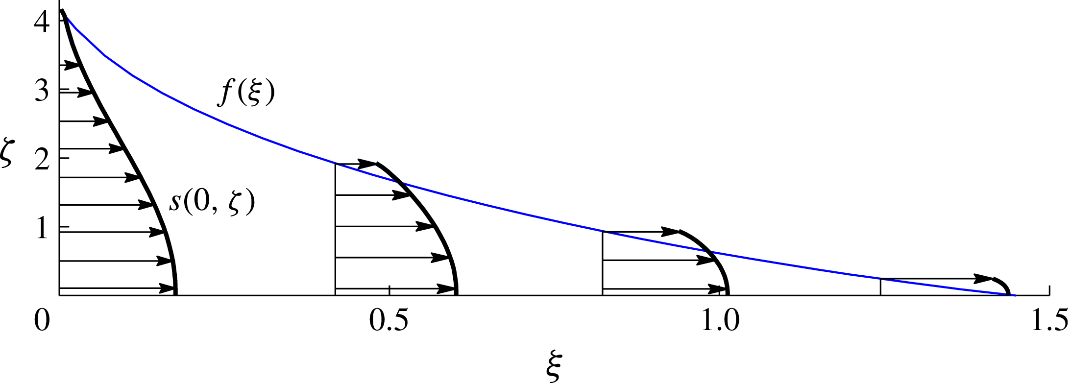
The solutions for a range of distribution parameters $n$ from 0.25 to 4 are shown in figure 9. The solutions show that the surfaces of constant density slope downwards in the direction of the flow. This is different to the situation found for a constant-volume release in § 3, where isopycnals are universally horizontal. Only the isopycnal along the base is horizontal in the present situation. The heaviest fluid therefore lines the base of the current. Note that this property does not necessarily apply to gravity currents with variations in viscosity, as has been illustrated by Woods & Mason (Reference Woods and Mason2000) for certain two-layer currents.

The case $n=4$ has a broadly linear, slightly convex shape similar to that which applies to a continuously injected gravity current of uniform density (Huppert & Woods Reference Huppert and Woods1995). As $n$ is reduced further, the current becomes fully concave once $n\leqslant 2.8$ . The numerical solutions indicate that a transition to a slope of infinite gradient near the input occurs at $n\approx 1$ and to an infinite height for $n\approx 0.5$ (precise estimates of these transitional values of $n$ were difficult to ascertain numerically because of the singularity in the height profile at ${\it\xi}=0$ ).

A selection of horizontal velocity profiles $s({\it\xi},{\it\zeta})$ for the illustrative case $n=1$ are plotted in figure 11. It is found that the horizontal velocity varies with vertical position $z$ . This contrasts with all uniform-density gravity currents in porous media, which have vertically invariant velocity fields. These properties are consistent with the result (2.7), which implies that vertical variations in horizontal velocity occur only if there are horizontal gradients in density present. At the input ${\it\xi}=0$ , we see that the velocity profile varies significantly from a maximal value at the base to a value of zero at the top. This is expected because the fluid at the top of the current has zero relative density [ $c(0,f(0))=0$ ] and is therefore stagnant. The vertical gradient of the horizontal velocity $\partial u/\partial {\it\zeta}=0$ along the base ${\it\zeta}=0$ , which is consistent with (2.9) and the fact that $c=1$ along ${\it\zeta}=0$ .

Interestingly, there is some variation in the rate of horizontal propagation for different values of $n$ , contrasting with the result that the rate of horizontal propagation is independent of distribution for a fixed release, found earlier in § 3.1. This variation is illustrated by the inset of figure 10(a), which shows an enlargement of the frontal positions. We see that the case $n=\infty$ maximizes the value of ${\it\xi}_{N}$ and hence the rate of horizontal propagation. Possible variation in ${\it\xi}_{N}$ is remarkably small, with a difference of just 3 % between the cases $n=\infty$ and $n=0.1$ . (Calculations for a selection of distributions not of the power-law form (4.11) were also found to lie within this range of ${\it\xi}_{N}$ .) The conclusion that horizontal propagation is independent of distribution thus holds to good approximation, if not exactly, for the case of a continuous input.

Figure 12.

Cross-sectional schematic of our experimental Hele-Shaw cell.

5 Experimental study

We conducted a laboratory experiment to compare with our theoretical predictions in the case of a constant-volume release. This was performed in a Hele-Shaw cell made of two polycarbonate sheets of length $100~$ cm and height $50~$ cm, forming a porous medium of porosity ${\it\phi}=1$ and permeability $k=b^{2}/12=7.8\times 10^{-4}~\text{cm}^{2}$ , where $b\approx 0.097~$ cm is the gap width (see figure 12). As working fluids, we used fresh water of density ${\it\rho}_{0}\approx 0.999~$ g $~$ cm $^{-3}$ , dyed using blue food colouring to a concentration of 4 vol%, and slightly salty water (saline) of density ${\it\rho}_{a}\approx 1.023~$ g $~$ cm $^{-3}$ , creating a maximum density difference of ${\rm\Delta}{\it\rho}\equiv {\it\rho}_{a}-{\it\rho}_{0}=0.024~$ g $~$ cm $^{-3}$ . The densities were measured using an oscillating U-tube densitometer to an accuracy of within $10^{-5}~$ g $~$ cm $^{-3}$ . The viscosity of the dyed water and saline were measured as ${\it\mu}=0.998\times 10^{-2}~$ P and ${\it\mu}_{a}=1.045\times 10^{-2}~$ P using a U-tube viscometer, and thus equal to within 5 %. The current was prepared from an equal mixture of fresh water and saline (see below) and hence the mean value $\bar{{\it\mu}}=1.022\times 10^{-2}~$ P was taken as the representative viscosity of the current.

To initialize a release of fluid, we formed a lock of horizontal length $10~$ cm between the left-hand edge of the cell and a thin strip of polycarbonate (the gate). The rest of the cell was filled with the clear saline solution. A series of eight layers of piecewise-uniform density were used to form the current behind the gate ( $N=8$ ), varying linearly in composition from the dyed fresh water to the clear saline solution. Beginning with the heaviest, the mixtures were injected sequentially behind the gate using a micropipette connected to a needle. This created the floating stratified fluid layer shown schematically in figure 12 and in the photograph of figure 13(a). With $V_{i}=V_{L}=10~$ cm representing the volume per unit width of each layer, and assuming an approximately linear relationship between composition and density, $c_{i}=i/N$ , the total relative mass per unit width of the current was evaluated as

(5.1) $$\begin{eqnarray}\displaystyle M_{0} & = & \displaystyle \mathop{\sum }_{i=1}^{N}c_{i}V_{i}{\rm\Delta}{\it\rho}={\rm\Delta}{\it\rho}V_{L}\mathop{\sum }_{i=1}^{N}\frac{i}{N}\end{eqnarray}$$

(5.2) $$\begin{eqnarray}\displaystyle & = & \displaystyle \frac{1}{2}(N+1){\rm\Delta}{\it\rho}V_{L}\approx 1.08~\text{g}~\text{cm}^{-1}.\end{eqnarray}$$

The experiment was initiated by removal of the gate, which released the region of buoyant stratified fluid. The buoyant current flowed along the top surface of the ambient fluid, differing slightly from the situation of a current flowing along a rigid boundary assumed in our theoretical development. By making the minor alteration of replacing the reduced gravity ${\rm\Delta}{\it\rho}g/{\it\rho}_{0}$ with the reduced gravity relevant to a floating fluid layer ${\rm\Delta}{\it\rho}g/{\it\rho}_{a}$ (e.g. Pegler et al. Reference Pegler, Kowal, Hasenclever and Worster2013b ), the relevant value of $U$ is found to be

(5.3) $$\begin{eqnarray}U\equiv {\it\rho}_{0}\left(\frac{{\rm\Delta}{\it\rho}}{{\it\rho}_{a}}g\right)\frac{k}{{\it\mu}}\approx 1.80~\text{cm}~\text{s}^{-1},\end{eqnarray}$$

where the factor in parentheses represents the replaced form of the reduced gravity.

Figure 13.

Photographs showing the evolution of the experiment from (a) its initial state, (b) after 50 s and (c) after 500 s.

A sequence of three recorded photographs is shown in figure 13 (the full sequence forms supplementary movie 1 available at http://dx.doi.org/10.1017/jfm.2015.733). The measured experimental frontal position is compared with the theoretical prediction (3.3), given dimensionally by

(5.4) $$\begin{eqnarray}x_{N}(t)=\left(9\mathscr{V}Ut\right)^{1/3}\quad \text{where }\mathscr{V}\equiv \frac{M_{0}}{{\rm\Delta}{\it\rho}}\approx 45~\text{cm}^{2},\end{eqnarray}$$

in figure 14. A comparison between the vertical thickness of the current, obtained by digitally detecting the outline of the current in the photographs, and the theoretical prediction of (3.15) with $n=1$ is shown in figure 15. There is generally excellent agreement with the data. From the images, it is evident that the isopycnals sustain a horizontal alignment, which is consistent with the prediction from § 3. The profiles are seen to approach the similarity solution gradually over time. The region of least buoyant fluid at the back of the current is observed to approach the similarity solution more gradually than elsewhere. The experimental frontal position $x_{N}$ initially lies ahead of the theoretical prediction because the current is released from an advanced state of finite horizontal length $x_{N}(0)=10~$ cm, while the time origin of the similarity solution (5.4) has the front of the current starting at the left wall ( $x_{N}(0)=0$ ). Based on the data of figure 14, the transition to the self-similar regime occurs over a time scale of approximately 10 s. The experimental flow front lies slightly less advanced than predicted by the theory. This may be attributed to the viscous drag caused by vertical shear between the current and the ambient fluid, which is neglected in our idealized theory. The need to drive a large-scale return flow of the ambient fluid underneath the current may have further contributed to the slight reduction in frontal speed compared to the prediction.

Figure 14.

Comparison between the measured frontal positions (black circles) and the theoretically predicted position (line) given by (5.4) on a log–log scale.

Figure 15.

Comparison between the experimental thickness profile $H(x,t)$ (solid curves) and the theoretical prediction (dashed curve), plotted in terms of the similarity variables defined by (3.3) and (3.4). The experimental thickness $H(x,t)$ was measured by digitally detecting the outline of the current from the experimental photographs. The theoretical prediction (dashed) is given by (3.15) with $n=1$ . No fitting parameters are used.