Introduction
As the demand for broadcast and wireless communication technologies is increasing day by day, the necessity of planning a new type of antenna with features like broader impedance bandwidth and highly directive radiation pattern has increased. Directional antennas are mostly used in applications to enhance the wireless systems' capacity and to reduce the effect of co-channel interference and multipath effects. Wideband antennas are used in different applications like satellite communication, RADAR, microwave imaging systems, remote-sensing systems, GPR detection, and medical applications. On the other hand, wideband antennas are also found useful in broadband communication to replace the need for multiple antennas for diversified applications due to its features like less complexity, lower power consumption, and a more compact footprint. Vivaldi antennas has been found as is one of the suitable candidates for a broadband directional communication system.
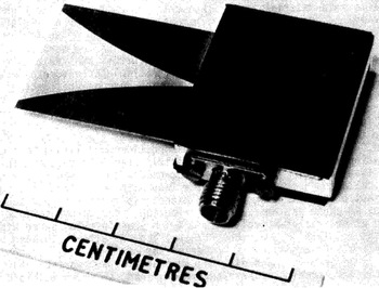
Gibson [Reference Gibson1], in the year 1979, first introduced the Vivaldi Antenna, which belongs to the class of end-fire traveling antennas. The Vivaldi antenna offers the feature of a slot line in which edge separation of the slot line extends higher than X/2, where X is the length of the parameter. The non-resonant traveling wave mechanism of radiation of a Vivaldi antenna is produced by a higher-order Hankel function [Reference Gibson1]. The main requirement for the gain of the Vivaldi antenna is that the bounded wave phase velocity should be equal to or exceed the surrounding medium, which needs a continuous phase leading compensation of the traveling wave structure. The Vivaldi antenna provides end-fire radiation with a beam width approximately the same for E- and H-planes. For achieving constant beam width, the shape of the antenna is ultimately expressed in terms of the wavelength, which is a dimensionless quantity. The video receiver module in [Reference Gibson1] is designed using a Vivaldi antenna and an integrated broadband video detector unit. The designed curve is in the form used in Fig. 1 with Y = ± AePX, where Y represents the distance of half separation and X means the length parameter. The magnification factor P determines the bandwidth. The radiating conductor slot plane of Vivaldi antenna is designed on an alumina substrate using the following equation [Reference Gibson1].

where X and Y represent dimensions to a new origin at the radiator feed.
8–40 GHz Video Receiver Module shows a video receiver module operates in the range of 8–40 GHz [Reference Gibson1].

Vivaldi antenna belongs to a class of a periodic, gradually curved slow leaky end-fire traveling antenna. The different portions of the antenna radiate different frequencies, but the size of the radiating part becomes constant with wavelength. It has infinite bandwidth [Reference Yngvesson, Schaubert, Korzeniowski, Kollberg, Thungren and Johansson2], but due to transition in the feeding section, i.e. transition from the transmission line to slot line the bandwidth is reduced. Another property of a Vivaldi antenna is constant beam width with respect to frequency, but it is also dependent on the proper designing of the antenna. Two major concerns for designing a Vivaldi antenna operating in the microwave range are the transition in the feeding structure and the dimension and shape of the antenna to attain a concentrated beam width. The Vivaldi antenna is mostly fed by using a balanced slot line. Some researchers use substrates with high dielectric constants and a small hole to connect the conductor. The process of tapered transition from microstrip to symmetric slot line and Vivaldi antenna with the change from microstrip to symmetric double-sided slot line is shown in Fig. 2.
Transition from microstrip to symmetric slot line and Vivaldi antenna [Reference Gazit3].
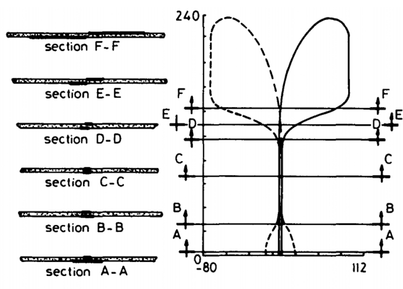
The transition in the feeding structure is done by tapering the microstrip line. Due to the transition in the feeding structure, the antenna produces low return loss over an extensive frequency range. The antenna also provides restrained beam width due to tapering of the slot line in the exponential form. To reduce the sidelobe gain, the end of the antenna should be curved. There are three areas namely feed area, transit area, and radiation area found in Vivaldi antenna. For electromagnetic coupling, the feed area is responsible. A modified structure of the antenna was developed by Gazit [Reference Gazit3] to overcome the drawbacks of the Exponential Tapered Slot Antenna (ETSA) [Reference Gibson1], which was known as the antipodal Vivaldi antenna (AVA). The bandwidth of ETSA can be enhanced by using the AVA because of its feeding technique, e.g. microstrip line-to-double-sided parallel stripline. Another type of Vivaldi antenna was introduced by Langley et al. [Reference Langley, Hall and Newham4] to overcome the drawbacks of AVA. The antenna is known as balanced AVA (BAVA). This antenna has the widest bandwidth, but the main disadvantages are its high cost and intricate design. They have been extensively used in different fields such as satellite communications, radars, microwave imaging systems, remote-sensing systems, and medical field for detecting tumor cell and cancer cell and telescopes.
Feeding mechanism of Vivaldi antennas
In Vivaldi antennas, the power transfer between a source and antenna is done through a feed line. In general, the characteristic impedance of a transmission line is 50 Ω. By maximum power transfer theorem, the Vivaldi antenna should be fed at a point where input impedance is 50 Ω for full input power. There are various feeding techniques for the Vivaldi antenna to match this condition. In [Reference Liu, Zhou, Yang, Li, Li and Yang5], a tapered microstrip feeding line with a fixed port width of 1.5 mm is adopted for perfect impedance matching. A feed transition structure is utilized to feed AVA, which is designed with a broad working band and low insertion loss in [Reference Wang, Yin, Wu and Lian6]. This transition from broadside parallel stripline to coplanar waveguide (CPW) makes this AVA cooperate reasonably with integrated microwave circuits. A compact tapered bending microstrip line feed is used in [Reference Natarajan, George, Kanagasabai and Kumar Shrivastav7] to provide wide impedance matching. The feed line consists of two metallic bending lines on both sides of the substrate. The feed design for the antipodal TSA found in [Reference Siddiqui, Antar, Freundorfer, Smith, Morin and Thayaparan8] comprises sections, as shown in Fig. 3, consisting of an elliptically contoured ground plane, a microstrip line, and a parallel plate, thus forming the balun transformer for broadband matching. A similar approach is used in [Reference Zhang, Liu, Wang, Yang and Shi9] with a microstrip-to-slot line transition balun exciting the Vivaldi antenna for a broadband impedance matching.
Schematic of an antipodal TSA using balun transformer as feed with W = D + 8, D = 2R 1 + E, L = 2R 2 + l s + l p + l t + l m + 4, R 1 = 68, R 2 = 1.3R 1, E = 2R 1 + 2, r 1 = 43.2, r 2 = 27, (x 1, y 1) = (2.975, 60), (x 2, y 2) = (12, 110), (x 3, y 3) = (69, 126.6), l s = 66.6, l p = 10, l t = 42.5, l m = 7.5, w p = 5.95, w m = 4.65, w gp = 60, g t = 8 (all parameters are in mm) [Reference Siddiqui, Antar, Freundorfer, Smith, Morin and Thayaparan8].

An exponential tapered microstrip line is implemented in [Reference Biswas, Ghatak and Poddar10] for excitation of a nature fern inspired fractal leaf structured antenna. A transition with an exponential form factor between the feed line and the radiator is introduced here which affects the impedance bandwidth. In [Reference Abbak, Akınc, Çayören and Akduman11], a microstrip feed, which is centered with respect to the exponential flares of the corrugated Vivaldi antenna, is utilized with a radial open stub at the end to increase the input impedance bandwidth. A conventional AVA is fed through a microstrip line in [Reference Moosazadeh, Kharkovsky, Case and Samali12] with a width of 1.14 mm to match with the 50 Ω coaxial line to achieve optimum bandwidth for detection of a void inside concrete structures. The structure of a compact Vivaldi antenna with a simple coaxial feed for wideband application is seen in [Reference Zhang, Chen, Tian, Liu and Liu13]. In [Reference Yang, Hoang, Bao, McEvoy and Ammann14], a two-stage coupled bandpass filter is implemented in the feed and terminated with a K-type connector, which is connected to two open shunt stubs, for low insertion loss, proper impedance matching, and sufficient bandwidth. In [Reference Yang, Zeng, Liu and Pan15], a new stepped connection feed structure between slot line and tapered patches is adopted in a planar printed Vivaldi antenna. By using the stepped connection structure, the impedance matching is significantly improved, and wide bandwidth is achieved. A highly directed Vivaldi antenna structure is obtained in [Reference Gao, Li, Zhang and Guo16] where the radiator is fed by a tapered microstrip line and slot line for impedance transformation from 50 Ω to about 80 Ω. In [Reference Yin, Yang, Yu and Gao17], a microstrip line to a symmetric double-sided slot line formation is used, which makes the input impedance conveniently matched to 50 Ω within a broadband. In [Reference Natarajan, Gulam Nabi Alsath, Kanagasabai, Bilvam and Meiyalagan18], the design of a three-port diversity antenna capable of producing three-directional radiation pattern for vehicular communications is presented. The proposed antenna consists of three uncorrelated Vivaldi antennas with three individual coaxial feeds developed on a single printed circuit board which offers ultra-wideband (UWB) characteristics with end-fire radiation pattern leading to high realized antenna gain. In [Reference Meng, Wu, Huang and Wu19], a conventional Vivaldi antenna is excited by a balun which consists of a T-junction power divider and two transition structures. The two transitions are a microstrip to CPW transition and a microstrip to coplanar stripline transition that are adopted to achieve wideband phase and magnitude balance resulting in wideband radiation performance. In [Reference Dzagbletey, Shim and Chung20], a two-stage quarter-wave balun structure is implemented at the feed point of two orthogonally crossed Vivaldi antennas to achieve UWB property as seen in Fig. 4.
Two-stage quarter-wave balun with l 1 = 26.7 mm, l 2 = l 3 = 11.7 mm, l 4 = 17.2 mm, w 1 = 1.65 mm, r 1 = 7.1 mm, r 2 = 6.7 mm. (a) Detailed geometry of balun. (b) Front/back view of the antenna [20].

In [Reference Lin, Wang, Deng and Zhang21], a conventional Vivaldi antenna is fed by a balun consisting of two different forms of transition structures. The first transition is realized by connecting the microstrip line to the slot line through short-ended via and the second transition is achieved by introducing electromagnetic coupling between the slot line and the output microstrip line. With the adoption of the balun structure, the unbalanced signal to balanced signals transition is achieved, leading to wideband performance. The antenna structure proposed in [Reference Song and Zhou22] consists of two orthogonal Vivaldi antenna elements, and the mode of feeding adopts electromagnetic coupling from the microstrip line to slot line. The improved balun can avoid the intersection of transmission lines, reduce the size, and simplify the assembly. A novel compact end-fire AVA is proposed for UWB applications in [Reference Pandey, Verma and Meshram23]. A bending feed line structure and sinusoidal modulated Gaussian tapered slot are employed to make the antenna compact. In [Reference Yao, Cheng, Wang, Yu and Chen24] a novel high gain circularly polarized (CP) antenna array for 5G applications is presented. The array element is an antipodal curvedly tapered slot antenna (ACTSA) producing CP field. The CP ACTSA fed by substrate-integrated waveguide is suitable to incorporate with substrates.
Balanced and unbalanced AVA
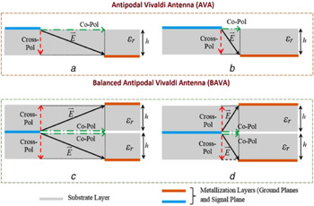
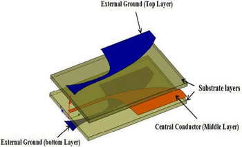
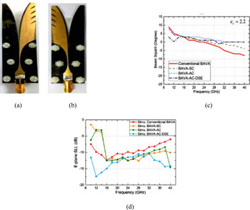
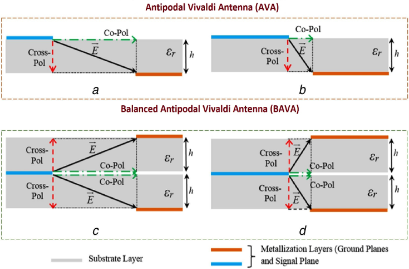
The BAVA as proposed by Langley et al. [Reference Langley, Hall and Newham4] incorporates an ultrawide bandwidth transition and overcomes the poor polarization performance of the basic unbalanced antipodal form [Reference Gazit3]. The structure of BAVA consists of three copper layers with the outer two copper layers acting as ground layers and the middle layer as a conductor. All copper layers are separated by substrates. As seen in Fig. 7, this structure equipoises the loading of dielectric material in between conductor and ground plane. Due to this balancing, changes in beam direction due to frequency, polarization, or orientation (called beam squint [Reference Bourqui, Okoniewski and Fear25]) are highly reduced as can be seen from Fig. 5. In [Reference Wang, Zhang, Wen and Sun26], the BAVA having an elongated substrate is loaded with slots resulting in increased end-fire performance and a higher front to back ratio. In [Reference Etesami, Khorshidi, Shahcheraghi and Yahaghi27], BAVA with transformation optics is used to enhance the gain, sidelobe level, and cross-polarization. Antenna gain and beam tilting can be refined by introducing a patch in between two flares of a BAVA, as seen in [Reference Li, Xia, Liu and Yang28]. In [Reference Wang, Fang, Chou, Qi and Xiao29], the beam squint can be lowered prominently by eliminating substrate in between two copper flares of the BAVA. Table 1 lists the performance comparison of BAVA design (Fig. 6).
Schematic representation of co-polarized and cross-polarized components of the electric field vector in AVA and BAVA [Reference Sarkar, Saha, Shaik, Siddiqui and Antar30].
Structure of balanced antipodal Vivaldi antenna (BAVA) [Reference Etesami, Khorshidi, Shahcheraghi and Yahaghi27].

Effect of balanced AVA. (a) Front view, (b) back view, (c) beam squint, (d) side lobe level (SLL) [Reference Wang, Fang, Chou, Qi and Xiao29].

Comparison of balanced antipodal Vivaldi antennas

Moreover, a compact BAVA with corrugation is observed in [Reference Wang, Fang, Chou, Qi and Xiao29]. Figures 7(a) and 7(b) show the top and bottom views of the typical fabricated BAVA, respectively. This BAVA is designed by using corrugation, slots, and by removing substrate present in between two flares. Figure 7(c) shows that the modified BAVA minimizes beam squint. BAVA with improved return loss and bandwidth is demonstrated in [Reference Wang, Wen, Zhang and Sun31]. A wideband BAVA is transformed to notch band BAVA in [Reference Sarkar, Saha, Shaik, Siddiqui and Antar30] by introducing a quarter wavelength spur line in the microstrip feed line. Four types of BAVA as conventional BAVA, BAVA with symmetric substrate cut-out (BAVA-SC), BAVA with asymmetric cut-out (BAVA-AC), and BAVA-AC with dual-scale slotted edges (BAVA-AC-DSE) are implemented here. An acceptable reduction in sidelobe levels can be seen in Fig. 7(d) by using BAVAAC-DSE.
Vivaldi antenna for wideband applications
In February 2002, the Federal Communications Commission (FCC) assigned 3.1 GHz from 10.6 GHz to UWB spectrum for public use [32]. UWB is an alternative for narrowband technology. Since 2002, UWB technology has been recognized as one of the most indispensable and a foremost choice in wireless technologies that assures to revolutionize high data rate transmission. It enables the personal area networking industry leading to innovations and greater quality of services to the end-users.
This technology has been utilized in different attractive applications, such as biomedical detection, ground-penetrating radar, etc. UWB communication systems and UWB indoor positioning systems have achieved significant development due to appealing characteristics in high-speed transmission rate and high multi-pathway resolution. Nowadays Vivaldi antenna gained considerable attention due to some attractive features such as planar structure, easy fabrication which is widely used for UWB applications. Because of its low cost and ease of integration, Vivaldi antenna is one of the best candidates used in most of the modern-day UWB applications. However, some of the antennas suffer from a large structure, high cross-polarization, feeding transition limitations as well as high sidelobe level.
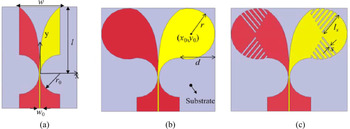
The antenna shown in Fig. 8 is used in UWB application. In this design [Reference Bai, Shi and Prather33], two circular-shaped loads are added on two arms of the antenna, as shown in Fig. 8(b). Slots of different lengths are etched on both arms of the antenna to improve radiation pattern and directivity of the antenna, as shown in Fig. 3(c). The tapered slots are expressed as:

Vivaldi antenna used in UWB application [Reference Bai, Shi and Prather33] with w 0 = 0.675 mm, r 0 = 11.6 mm, l = 40 mm, w = 24 mm, d = 20 mm, (x 0, y 0) = (16.559, 25.8), s = 0.9 mm, l s = 13.7 mm.

For the top and bottom layers, where w 0 is the width of the microstrip line and α is the exponential transition rate. The cut-off wavelength of the antenna depends on the aperture width of the antenna which can be expressed as

where w is the aperture width of the antenna and λc is the cut-off wavelength. The circular shape of flare with slots enhances bandwidth and low-frequency performance of the antenna. In [Reference Moosazadeh34], a dielectric cover made of Teflon (PTFE) with relative permittivity of 2.1, loss tangent of 0.0002, and thickness of 0.8 mm is used to make the AVA appropriate for different wideband applications. Due to this innovative design, the proposed antenna offers wider bandwidth, higher gain, lower sidelobe and cross-polarization levels, narrow E-plane half-power beamwidth, and improved F-to-B ratio. In [Reference Krishna, Madhav, Giridhar, Reddiah Babu, Sai Krishna and Mohan Reddy35], an AVA is presented for wideband application. In this design, dual tapered slot edge is placed on both the arm of the antenna. Due to these slots, the antenna provides wide operating bandwidth, H-plane quasi-omnidirectional radiation pattern at lower frequency band and more directive radiation pattern in the E-plane at the high-frequency band. In [Reference Yang, Zeng, Liu and Pan15], a Vivaldi antenna for switchable and widely tuneable band-notch characteristics is proposed. In this design, one stepped-impedance resonator (SIR) is placed to achieve notched band and to achieve tuneable band-notch, varactor diodes are loaded. By controlling the DC bias voltage, the UWB notched band is achieved from 3.1 to 6.8 GHz. In [Reference Wang, Fang, Chou, Qi and Xiao29], a BAVA is proposed with an asymmetric substrate cut out and dual-scale slotted edges to eliminate the drawbacks of AVA and for different millimeter-wave applications. This design reduces the sidelobe and cross-polarization level, enhancing the gain of the antenna. In [Reference Wang, Wen, Zhang and Sun31], a wideband conformal end-fire antenna array mounted on a cylindrical structure provides ultra-wide bandwidth, low cross-polarization level, and wide 3 dB beam width. The effects of the antenna height with respect to the edge of the hollow conducting cylinder and slant angle of mounting the antenna elements on the conducting surface, on the radiation pattern of the antenna have also been examined. Array assembly offers high gain but side lobes are more and mutual coupling between array elements increases [Reference Tianang, Elmansouri and Filipovic36]. So different methods for reducing mutual coupling are essential to be employed [Reference Zhu, Liu, Chen and Wen37].
In [Reference Liu, Zhou, Yang, Li, Li and Yang5], tapered slot edge with resonant cavity structure is used in antenna design to improve the radiation performance of the antenna. Due to this structure, the operating bandwidth is increased by 14.6%. This structure also enhances the gain of the antenna at lower frequencies. In [Reference Wang, Yin, Wu and Lian6], elliptically shaped strip conductors are used in the antenna design to extend the lower operating frequency to enhance the radiation performance of the antenna and make the antenna suitable for wideband communication. The radiation performance of the antenna is also improved in the lower operating band by two pairs of tapered slots and circularly shaped loads. The lower cut-off frequency f 0 of the antenna can be determined using the following equation [Reference Wang, Yin, Wu and Lian6]:

Here, wp represent the width of the two arms of the antenna, ɛr is the dielectric constant of the proposed antenna. In [Reference Elsheakh, Eltresy and Abdallah38], a conventional antipodal Vivaldi for UWB wireless communication is presented. Two slots are etched on the ground plane to achieve wider bandwidth, and to increase the bandwidth further, circular grooves as electromagnetic band-gap structure are engraved on the antenna design. Double layer of Vivaldi antenna ground plane is used to enhance the gain of the antenna. A parasitic meander-shaped structure is introduced in the antenna to make the Vivaldi antenna appropriate for UWB application, as given in [Reference Elsheakh and Abdallah39]. The antenna provides bandwidth from 4.5 to 12 GHz. A PIN diode is introduced in the structure to add or remove the UHF bands. In [Reference Natarajan, George, Kanagasabai and Kumar Shrivastav7], microstrip to tapered transition feed structure Vivaldi antenna is presented. An L shape structure is etched on the radiation fins to enhance the bandwidth of the antenna and make the antenna suitable for UWB communication. A compact AVA for UWB application is presented [Reference Hood, Karacolak and Topsakal40]. It provides low cross-polarization level and good gain over the entire frequency range. In [Reference Siddiqui, Antar, Freundorfer, Smith, Morin and Thayaparan8], a tapered slot AVA is designed. In this design, elliptical strip conductors are used in feeding structure. Due to this, the antenna becomes an appropriate candidate for UWB applications. This antenna also offers directional radiation in end-fire direction. The comparison between different Vivaldi antennas used in UWB application is given in Table 2.
Comparison of different Vivaldi antennas used in wideband application

Dispersion characteristics of Vivaldi antenna for wideband applications
Besides return loss and radiation efficiency, the dispersion characteristic is one of the most important factors which should be considered in wideband applications. In contrast, the conventional parameters are sufficient to evaluate the performance of a narrowband antenna. Still, in the wideband applications, these parameters are inadequate for the applicability of the antenna. The wideband antenna transmits pulses with distortions, and the antenna performance should be evaluated using dispersion parameters, i.e. transfer function, group delay, and fidelity factor as well. The dispersion characteristics of a Vivaldi antenna can be calculated by proper transmission/reception setups. The frequency-domain dispersion characteristics of the antenna are the transfer function (S 21) and group delay. In Tx/Rx setup, the received signal spectrum is attained as follows [Reference Mehdipour, Mohammadpour-Aghdam and Faraji-Dana41]:

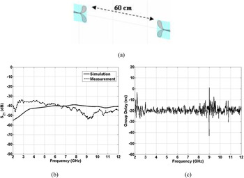
where S t(f) is the transmitted spectrum and S 21 is the transfer function of the signal. With a weak distortion in the magnitude and phase of the transfer function, the received signal will have less dispersion. The phase distortion can be estimated by representing the group delay parameter as−dϕ/df where ϕ is S 21 phase. A nearly constant group delay leads to the linearity of phase. In Tx/Rx setups, two antennas should be oriented in a specific direction, as shown in Fig. 9(a). It is due to this fact that the Vivaldi antenna is an end-fire directive antenna and the propagation takes place from the slot surrounded by two radiation elements. Two similar antennas are placed at a separation distance of 60 cm. The 60 cm distance (at the lowest operating frequency approximately 6λ) is selected to have each antenna within the far-field region of the other one. The simulated/measured transfer function and group delay of the Vivaldi antenna are illustrated in Figs 9(b) and 9(c), respectively. The measurement and simulation results are observed to be in good agreement with one another. Furthermore, the behavior of S 21 and group delay is seen to be acceptable in the required frequency range of 3.1–10.6 GHz.
Simulation setup and transfer function for Vivaldi antenna. (a) Tx/Rx setup, (b) magnitude of S 21, (c) group delay [Reference Mehdipour, Mohammadpour-Aghdam and Faraji-Dana41].

The time-domain characteristic [Reference Mehdipour, Mohammadpour-Aghdam and Faraji-Dana41] of Vivaldi antennas being one of the most important factors has been analyzed here. In Fig. 10, the transmitted and received signals of the Vivaldi antenna have been represented where the shapes of the pulse show that the transmitted pulse distortion is not considerable. The amount of pulse distortion induced by the antenna can be validated by the fidelity factor (F) between the received signal and the transmitted signal which is defined by:

where S t(t) and S r(t) are the transmitted and received signals, respectively. F represents the similarity between two signals. With two similar signals, F coefficient becomes unity. Using equation (6), the fidelity factor between transmitted and received signals in Tx/Rx setups between two identical antennas has been calculated [Reference Mehdipour, Mohammadpour-Aghdam and Faraji-Dana41] which yields a fidelity factor of 0.7904. As we know, because the Vivaldi antenna has no omnidirectional applications [Reference Gibson1], the transmission/reception performance of the antenna in one direction has been considered.
Transmitted and received signals in Tx/Rx setup [Reference Mehdipour, Mohammadpour-Aghdam and Faraji-Dana41].

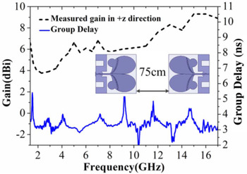
Two identical proposed AVAs in this letter [Reference Wang, Yin, Wu and Lian6] are placed face to face with a distance of 75 cm, as shown in Fig. 11. The measured group delay varies around 3.4 ns with a fluctuation of 0.6 ns in most frequencies, which means this antenna can transmit and receive signals without severe distortion in the whole operating band.
Measured gain in end-fire direction and group delay [Reference Wang, Yin, Wu and Lian6].

Dispersion characteristics of a compact AVA [Reference Natarajan, George, Kanagasabai and Kumar Shrivastav7] in terms of group delay are measured and shown in Fig. 12. Almost flat response is noticed over the operating bandwidth, which indicated minimal distortion in the transmitted pulse.
Measured group delay [Reference Natarajan, George, Kanagasabai and Kumar Shrivastav7].

In [Reference Hood, Karacolak and Topsakal40], a compact AVA for UWB applications is proposed. Both the plots in Fig. 13 show the dispersion characteristics of the antenna with a discontinuity at 3.55 GHz, possibly due to the resonance at that frequency in the operating bandwidth.
(a) Phase response of the fabricated FR4 antenna. (b) Group delay of the fabricated antenna [Reference Hood, Karacolak and Topsakal40].

The simulated time-domain response of a UWB antipodal TSA [Reference Siddiqui, Antar, Freundorfer, Smith, Morin and Thayaparan8], when excited with a Gaussian pulse covering the entire frequency spectrum, can be observed in Fig. 14 [Reference Siddiqui, Antar, Freundorfer, Smith, Morin and Thayaparan8]. The received pulse was obtained by placing an E-field probe in the far-field of the antenna at 10 m oriented along the x-direction. The originally transmitted pulse full-width at half-maximum (FWHM) was 180 ps, while the received pulse on the x-oriented E-field probe had an FWHM of 187 ps. The fidelity factor was calculated at 0.94.
Simulated transmitted pulse and received pulse on the E-field probe at the far-field of the antipodal TSA [Reference Siddiqui, Antar, Freundorfer, Smith, Morin and Thayaparan8].

Fractal-based Vivaldi antenna
Fractal is a structure which is repeated but not predefined [Reference Kumar and Nath42]. This type of construction consists of multiple self-copies at various levels. Using fractal geometry, the space occupied by the antenna can fill in a more effective manner than any traditional Euclidean antenna. For example, we have discussed the geometric construction of the standard Koch curve, which is simple that starts with a straight line as an initiator. Then it is partitioned into three equal parts, and the segment at the middle is replaced with two others of the same length which is the first iteration of the geometry which is called the generator [k 0]. This process is reused in the generation of higher iterations where successive iterations contain a smaller bump on each side of the first bump, and the sides of every triangle are same. Figure 15 shows different iterations Koch fractal shape for a given indentation angle “θ” where the indentation angle “θ” is taken as a design parameter and its value is chosen as 60° for conventional Koch fractal curve.
Steps for construction of conventional Koch curve geometry [Reference Kumar and Nath42].

The dimension of the Koch fractal geometry can be calculated by the following equations [Reference Kumar and Nath42]


The perimeter after n th iterations is:

where Lθ is the side of the generator.
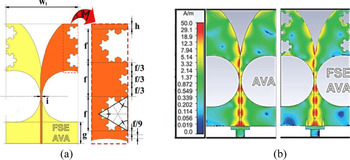
AVA with Koch shape fractal on radiator and ground is shown in Fig. 16. In [Reference de Oliveira, Justo, Perotoni, Kofuji, Neto, Bueno and Baudrand43] to make the antenna suitable for different medical imaging applications, the Koch fractal structure is used in the radiator and ground plane of the antenna. Due to the presence of fractal slot edge, the lateral E-fields are suppressed in the surroundings of the fractal structure because the fractal slot edge makes the interface between the metal edge and medium become softer. Figure 16(b) shows the surface current distribution of AVA and fractal slot edge AVA. The presence of the fractal structure on the edge of the antenna rejects the trapping of E-field, which is observed in the AVA. The presence of fractal-shaped ellipse structure in AVA improves the gain of the antenna over the entire frequency range, which makes the antenna an ideal candidate for different UWB and imaging applications.
Antipodal Vivaldi antenna with fractal structure. (a) Antenna structure with a = 4.03 mm, b = 11.17 mm, c = 18.15 mm, d = 23.02 mm, e = 59.81 mm, f = 7.00 mm, g = 9.97 mm, h = 1.00 mm, i = 1.00 mm, r = 13.12 mm, w 1 = 36.30 mm, w 2 = 21.35 mm. (b) Current distribution [Reference de Oliveira, Justo, Perotoni, Kofuji, Neto, Bueno and Baudrand43].

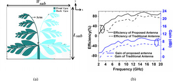
In [Reference Biswas, Ghatak and Poddar10], a new type of fractal structure known as fern leaf fractal structure is applied in the AVA design, as shown in Fig. 12(a).

Equation (10) is used to design the radiator and ground plane of the antenna. Where w 0 represents the width of the feed line and a 1 denotes the rate of tapering given in equation (6)

In equation (11) L 1 is the radiator length and Ld is the flared distance. In Fig. 17(a) Lsub and Wsub represent the length and width of the antenna, respectively. In the antenna structure, θ 1 and θ 2 represent the rotation angles. The second iteration of this fractal structures improves the bandwidth of the antenna by reducing the lower cut-off frequency. The proposed antenna also provides a fractional bandwidth of 175%. The designed antenna also produces higher gain over the entire frequency range, as shown in Fig. 17(b). In [Reference Karmakar, Bhattacharjee, Saha and Bhawal44], a novel fractal inspired AVA is proposed for wideband applications. First, a parasitic fractal lens is introduced in the flare aperture section of the AVA to improve its performance. But the presence of parasitic lens does not influence the performance of the antenna at a higher frequency range. Now to adjust the gain and radiation pattern of the antenna at high frequencies, a Koch fractal shape dielectric director as an extension of the antenna substrate is used to improve the gain of the antenna.
(a) Antipodal Vivaldi antenna with a fern-inspired fractal structure with L sub × W sub = 50.8 × 62 × 0.8 mm3. (b) Gain improvement using fractal structure [Reference Biswas, Ghatak and Poddar10].

The comparison of different fractal-based Vivaldi antenna is given in Table 3. The fractal structure makes the antenna layout complex. Still, the presence of the fractal structure makes the antenna innovative as well as improves the radiation performance of the antenna without occupying more geometrical area. The advantages of using fractal shape in the antenna design are that it enhances the performance of the antenna without increasing antenna dimensions. The fractal layout on the edge of the radiator and the ground plane of the Vivaldi antenna reduces the sidelobe level and also improves the directivity.
Comparison of different fractal-based Vivaldi antennas

Vivaldi antenna for microwave imaging application
Nowadays, microwave imaging [Reference Moosazadeh, Kharkovsky and Case45] technique is widely used in different detection application. In this imaging technique, first, a microwave signal is transmitted to the targeted object. Then the signals reflected from the object are tested to reconstruct images of the targeted objectives. In this application, the antenna plays a vital role with high directivity, and improved radiation characteristics are used.
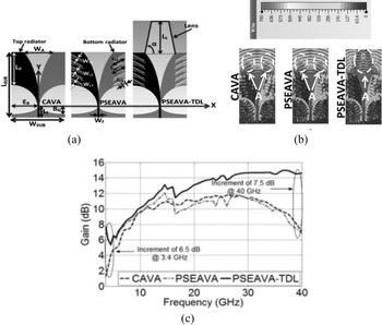
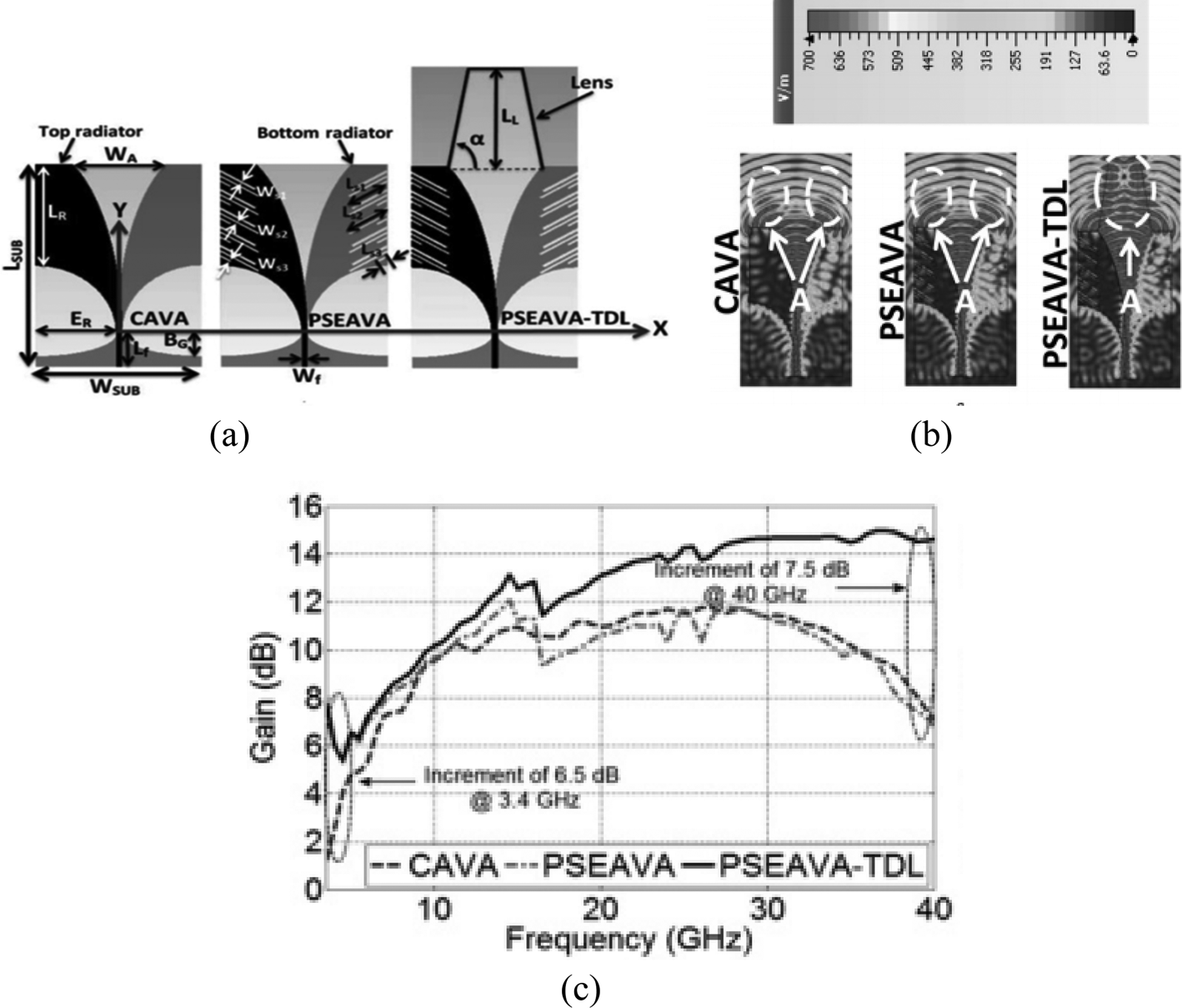
The antenna design, as shown in Fig. 18, is used for imaging of different construction materials [Reference Moosazadeh, Kharkovsky and Case45]. In this design, a trapezoidal shape dielectric lens, as shown in Fig. 18(a) is used in the aperture of the antenna to improve radiation properties making it suitable for imaging of different construction materials. Figure 18(b) shows the electric field distribution of the proposed antenna. The presence of the trapezoidal shape dielectric lens concentrates most of the electric field in the desired direction, i.e. along the y-axis direction. The improvement of the gain of the antenna due to the presence of a dielectric lens is given in Fig. 18(c). In [Reference Moosazadeh and Kharkovsky46], rectangular-shaped slits are introduced on the radiator and ground of the antenna to achieve wide impedance bandwidth. A half-circular shape dielectric lens is also introduced in the antenna design to achieve high directivity and front-to-back ratio. Due to these features, the antenna is appropriate for imaging of cracks inside concrete. A corrugated Vivaldi antenna is proposed in [Reference Abbak, Akınc, Çayören and Akduman11] for microwave imaging applications. In this design, due to the presence of grooves, the antenna provides improved radiation performance. In [Reference Pandey, Singh, Bharti, Pandey and Meshram47], a Vivaldi antenna with a corrugation structure on the radiating portion is presented. In this design, grating elements are also loaded near the tapering part of the antenna to achieve higher gain and improved radiation pattern in the end-fire direction. Due to these features, the antenna can be used in microwave imaging. In [Reference Mahmud, Islam, Rahman, Alam and Samsuzzaman48], a novel Vivaldi antenna with several slots etching on the radiation fins is presented. These slots reduce the size of the antenna and also provide wider bandwidth, higher gain, and improved directivity. The slots also make the antenna highly efficient. Due to its compact structure and attractive features, the antenna is used in different medical imaging applications. In [Reference Juan, Guang, Lin and Demin49], a balanced AVA is presented for microwave imaging applications. In this design, exponentially tapered corrugation edge and elliptical shape director is used to enhance the radiation characteristics. The elliptical shape dielectric director improves the gain of the antenna over the entire frequency range and also produces a directive radiation pattern which makes it appropriate for an imaging application. An AVA in [Reference Moosazadeh, Kharkovsky, Case and Samali12] is proposed for detecting void inside the concrete. Here, to improve the gain of the antenna at high as well as lower frequencies, rectangular shape slit and a dielectric director of half elliptical shape are used in the antenna design.
Antipodal Vivaldi antenna for imaging application. (a) Antenna structure with L SUB = 60 mm, W SUB = 40 mm, L R = 30 mm, B G = 6.80808 mm, L f = 10 mm, < ddollar > <ddollar > E R = 19.405 mm, W A = 22.84 mm, L L = 30 mm, W f = 1.19 mm, d = 78.71°, W s1 = 0.8 mm, L s1 = 9 mm, W s2 = 0.6 mm, L s2 = 9.8621 mm, W s3 = 0.6 mm, L s3 = 2.84615 mm, (b) electric field distribution, (c) gain characteristics [Reference Moosazadeh, Kharkovsky and Case45].
The proposed antenna is used to obtain the depth of penetration of concrete specimen and wideband microwave imaging application, as demonstrated in Fig. 19. The antenna is attached to the scanning machine keeping a particular gap to obtain the 3D and 2D images of the specimen. These specimens are generated using data and synthetic-aperture-radar-based algorithm. In this case, one of the 3-month-old concrete beams is used as a specimen to simulate the void, as shown in Fig. 19(a). The sample is scanned by using a 3 mm step size. The holographic slices of the 3D images are shown in Figs 19(b)–19(d).
Proposed antenna test the concrete beam: (a) top and side view; holographic slices of 3D images: (b) the top of insert, (c) 9 mm below the top insert, (d) 15 mm below the top insert [Reference Moosazadeh, Kharkovsky, Case and Samali12].

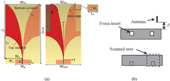
In [Reference Moosazadeh, Kharkovsky, Esmati and Samali50], an elliptically-tapered AVA with an operating frequency range from 1.65 to 18 GHz designed for microwave imaging applications is presented. It includes comb-shaped slits and elliptical opening in the top and bottom radiators. It is shown that the antenna gain has been increased by comb-shaped slits at lower frequencies up to 9.5 dBi at 2 GHz and at higher frequencies up to 14.2 dBi at 18 GHz. Comb-shaped corrugation on elliptical flare is applied in [Reference Moosazadeh, Kharkovsky, Case and Samali51] to efficiently find empty spaces in the concrete beam. The corrugation on flares increases gain and return loss of the AVA (Fig. 20).
(a) Conventional antipodal Vivaldi antenna and comb-shaped slits antipodal Vivaldi antenna with W SUB × L SUB = 120 × 202 mm2, W A2 = 84 mm, W 2 = 59.43 mm, L 1 = 229 mm, L 2 = 80 mm, W f = 1.14 mm, L f = 15 mm, W g = 50 mm, L g = 15 mm, W c = 1 mm, L c = 17 mm, B = 25. (b) Schematic of concrete beam with two foam inserts imaged by the proposed antenna at standoff distance d [d = 10 mm] [Reference Moosazadeh, Kharkovsky, Esmati and Samali50].

In [Reference Bah, Hong, Jamro, Liang and Kponou52], the design and implementation of a Vivaldi antenna (BAVA) and breast phantom for breast cancer imaging have been covered within the range of 3.1–10.6 GHz. Two different phantoms are made to simulate the scene. A dielectric constant relatively close to the real breast tissues has also been found. This design can be used in breast cancer detection without the need for any liquid coupling medium, which is required in many other applications (Fig. 21).
(a) Single parametric antenna [dimensions in “mm”]. (b) Antenna array surrounding the breast with the tumor in it [Reference Bah, Hong, Jamro, Liang and Kponou52].

In most of the cases, Vivaldi antennas play an essential role for imaging applications though in some of the issues it suffers from the deviated beam (E-plane) at upper frequencies as well as increased sidelobe levels at mid frequencies (Table 4).
Comparison of different Vivaldi antennas used in microwave imaging applications

Gain boosting techniques in Vivaldi antennas
Using dielectric director
Different researchers use a high permittivity dielectric material in the aperture center of the antenna known as dielectric lens or director to achieve wider bandwidth and higher gain [Reference Amiri, Tofigh, Ghafoorzadeh-Yazdi and Abolhasan53].
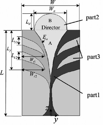
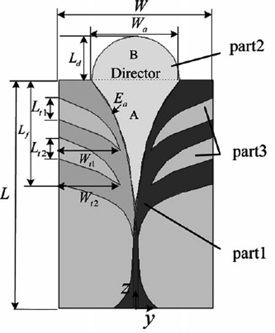
This method is also used in [Reference Juan, Guang, Lin and Demin49] where a half circular-shaped lens is used for gain enhancement, as shown in Fig. 22. The proposed antenna also used exponentially tapered corrugation slot edge on the radiator and ground plane. The presence of the rectangular shape slot edge and the director helps the antenna to achieve wider bandwidth, high directivity, and front-to-back ratio. The tapered slots also reduce co-polarization and cross-polarization [Reference Moosazadeh, Kharkovsky, Case and Samali54].
Antipodal Vivaldi antenna with dielectric director having L = 108 mm, W = 70 mm, W a = 42 mm, L d = 32 mm, L f = 72 mm, L t1 = 13.5 mm, L t2 = 11.8 mm, W t1 = 26 mm, W t2 = 26.5 mm [Reference Juan, Guang, Lin and Demin49].
In [Reference Moosazadeh, Kharkovsky, Case and Samali12], an exponential tapered AVA with a half elliptical-shaped dielectric lens as an extension of antenna substrate is used. The presence of this dielectric lens improves the gain of the antenna, and a regular slit edge extends the lower end bandwidth of the antenna to find application in different UWB applications. Hemisphere shape lens loaded in the antenna structure for different time-domain operation is given in [Reference Akhter, Abhijith and Akhtar55]. This hemisphere shape lens increases overall directivity of the antenna and also widens the bandwidth of the antenna. A trapezoidal shape dielectric lens is loaded in the major axis direction in [Reference Wan, Chen and Li56]. The presence of the dielectric director overcomes the shifting of the antenna peak gain problem and enhances the radiation performance of the antenna. In [Reference Moosazadeh and Kharkovsky57], a trapezoid shape dielectric director and periodic slit edge are introduced in the antenna to improve the radiation properties of the antenna. The high permittivity dielectric director reduces mutual coupling between the elements and beam tilting problem and concentrates the radiation in the end-fire direction. As a result, the antenna produces improved gain with the dielectric director.
A high permittivity material known as a director is used in [Reference Teni, Zhang, Qiu and Zhang58] to improve the radiation performance of the antenna. This director focuses most of the energy toward the aperture center and significantly improves the gain and directivity of the antenna. In [Reference Kota and Shafai59], a Vivaldi antenna with triangular shape dielectric lens is presented. In this design, due to the dielectric lens, the electrical path length is increased and transmitted wave delayed. Due to this delay, the radiated wave becomes parallel and produces more directed radiation pattern and improved gain. In [Reference Zhang, Chen, Tian, Liu and Liu13], a director and a convex lens are added in the wideband AVA design to improve the performance of the antenna at high frequencies. By using the dielectric lens with other performance improvement techniques like an array, slots, corrugation, etc., enhances the parameters of AVA very effectively [Reference Zhang, Li, Wang and Guo60]. The comparison of Vivaldi antennas with a dielectric director as the gain booster is given in Table 5. In most of the cases, dielectric directors found suitable for enhancing the antenna characteristics but achieving an appropriate shape of the director may be a challenging issue that can lead to the bulky structure of the antenna along with higher fabrication cost.
Comparison of Vivaldi antennas with dielectric director

Using dielectric slab
Dielectric slab placed on both sides of the antenna is a practical approach to enhance the gain of the Vivaldi antenna [Reference Li, Xu, Wang, Zhang and Lv61] but with a slight compromise of increasing antenna dimension. The dielectric slabs utilize the coupling between the antenna and dielectric sheets to overcome problems such as main beam tilt and split, high cross-polarization component, and low gain at high frequencies narrowing its gain bandwidth.
In [Reference Li, Xu, Wang, Zhang and Lv61], an innovative antipodal tapered slot antenna with double thin rectangular dielectric sheets (Fig. 23) is presented to achieve improved radiation properties. In [Reference Li, Pang, Wang, Zhang and Lv62], a simple dielectric slab placed on both the side of the Vivaldi antenna is proposed for improving the performance of the antenna. The dielectric slabs match space waves which are emitted from the CVA and then converted into surface waves which radiate in the end-fire direction. By using this method, the gain of the antenna increases without elongating the overall antenna length. Comparison of Vivaldi antenna design based on a dielectric slab is given in Table 6.
Antipodal Vivaldi antenna with a dielectric slab [Reference Li, Xu, Wang, Zhang and Lv61].

Comparison of Vivaldi antennas based on a dielectric slab

Using parasitic lens
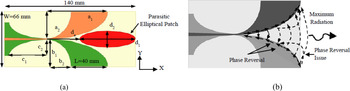
Different researchers have found that the herein method [Reference Nassar and Weller63] can be used to enhance the gain of the antenna. In this method, by introducing a parasitic element in the flare aperture section of the antenna, the gain is increased by focusing the radiation in the end-fire direction.
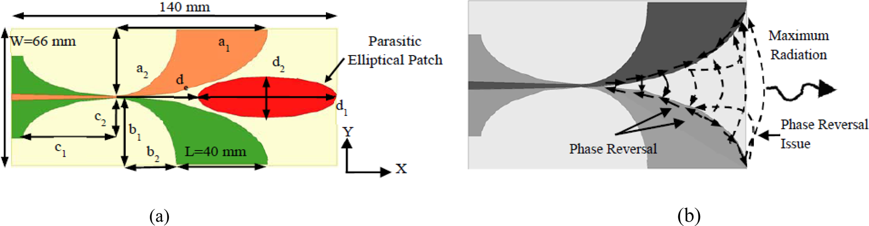
It is seen from Fig. 24 that a parasitic element is placed in the aperture section of a conventional AVA and it improves the field coupling between the arm of the antenna; as a result, it produces stronger radiation in the end-fire direction [Reference Nassar and Weller63]. By using this technique, the directivity and the high-frequency performance of the antenna are improved. The most important part of the broadband antenna is its long electrical length, but it reduces the performance of the antenna at higher frequencies due to phase reversal along the length. As shown in Fig. 19(b), due to phase reversal, off-axis radiation is created along with end-fire radiation from the aperture of the antenna. This problem of the broadband antenna can be overcome by minimizing the flaring length of the antenna. This reduction in the flare length enhances the lower operating frequencies.
(a) Antipodal Vivaldi antenna with parasitic lens having a 1 = 66 mm, a 2 = 33 mm, b 1 = 32 mm, b 2 = 26 mm, c 1 = 40 mm, c 2 = 20 mm, d 1 = 30 mm, d 2 = 10 mm, d e = 36 mm. (b) E-field distribution at high frequencies [Reference Nassar and Weller63].
In [Reference Li, Kang, Su, Guo, Yang and Wang64], an AVA with diamond shape parasitic lens is presented to improve the high-frequency gain. The presence of the lens enhances the radiation performance of the antenna at higher frequencies. In [Reference Eichenberger, Yetisir and Ghalichechian65], an elliptical-shaped parasitic element is introduced to reduce the sidelobe radiation and improve the directivity of the antenna. The presence of this element enhances the directivity and gain of the antenna. In [Reference Li, Xia, Liu and Yang28], a Vivaldi antenna is presented where a metal director is used to improve the gain and radiation pattern of the antenna. The presence of the director enhances the bandwidth of the antenna.
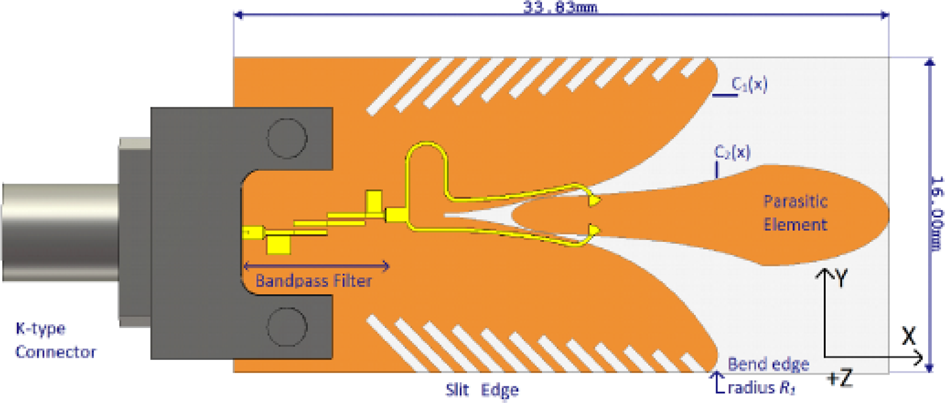
A dual-stub coplanar Vivaldi antenna with a parasitic element placed in the throat area and an integrated bandpass filter is shown in Fig. 25 [Reference Yang, Hoang, Bao, McEvoy and Ammann14]. The exponential curve applied to design the antenna is $C_{i( x ) } = {\pm} a_i \times e^{p_ix}$ where C i(x) is the exponential profile with a i = 0.15 and p i = 0.25. The presence of two semi-elliptical-shaped exponential curves with a parasitic element in the throat of the antenna structure provides better radiation performance. The slits present on the edge of the radiator and ground plane regulate the radiation performance of the antenna. In order to suppress the harmonics, the bandpass filter is introduced in the source end. The dependence on permittivity and thickness of dielectric material makes a constraint for the designers. Also, a dielectric lens slightly increases the weight. Comparison of the Vivaldi antenna design using the parasitic lens is given in Table 7.
Geometry of antipodal Vivaldi antenna with bandpass filter [Reference Yang, Hoang, Bao, McEvoy and Ammann14].
Comparison of Vivaldi antenna with parasitic lens

Vivaldi antenna with metamaterial
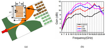
Metamaterials [Reference Sang, Li, Chen and Lv66] have some unique characteristics than those of other natural materials. It is a synthetic type of material which depends on structure such that it discloses some properties which are not usually found in natural materials, mainly a negative refractive index. Applications of metamaterials in microwaves are numerous and opened the door to new strategies in the design of microwave devices, also referred to as dispersion engineering, which considers and controls the phase response of devices. There are two main approaches in the design of microwave circuits using metamaterials: the resonant approach which uses thin wires, split-ring resonators (SRRs) and complementary split-ring resonators (CSRRs), and the transmission line approach based on dual transmission line theory. The first one leads to lossy and narrowband circuits, while the second, non-resonant approach, provides design tools for broad bandwidth devices with low loss. Metamaterials are used to improve the radiation properties of the antenna. The anisotropic zero-index metamaterial (AZIM) [Reference Bhaskar, Johari, Akhter and Akhtar67] is used to enhance the gain of the antenna.
In order to achieve a broadband gain, the high index metamaterial and anisotropic inhomogeneous artificial material are used [Reference Pandey, Singh and Meshram68]. Many researchers have found an impact on the characteristics of the antenna by using this type of materials. Metamaterial offers some surprising features. In antenna design, either unit-cell or multiple-cell metamaterials are used as an array. A unit cell is usually smaller than 1/10 of the operating wavelength, depending on the shape of the metamaterial, but the unit-cell size is different. The presence of metamaterial reduces the dimension of the antenna as well as improves the radiated power level, enhances the bandwidth and gain of the antenna. By using metamaterial as a radiating component, one can design an antenna of compact size for multiple communication systems. The metamaterial is used as an antenna environment to enhance the radiation properties of the antenna. The metamaterial is also used as part of the antenna component to miniaturize the size of the antenna without disturbing the performance. But the difficulty lies in designing metamaterial unit cells as well as low EM wave confinement within guiding structure and more moderate gain enhancement at lower frequencies.
As shown in Fig. 26, metamaterials are loaded in the aperture section of the AVA [Reference Sang, Li, Chen and Lv66]. The presence of the metamaterial unit in the antenna aperture section improves the gain of the antenna in the non-resonant frequency band, as shown in Fig. 26(b) [Reference Sang, Li, Chen and Lv66]. It can be observed that if the cell length is lower than the gain reduced at higher frequency as well as lower frequency. But when we add rows of metamaterial unit cells, then the gain increases drastically at the non-resonant frequency band. Parallel unit of metamaterials works as a phase shifter and enhance the radiation performance of the antenna. A compact high-gain AVA is presented in [Reference Zhang, Liu, Wang, Yang and Shi9]. Again, to enhance the main lobe radiation and the gain, the transverse slots are etched on the arm. A band-notched Vivaldi antenna with AZIM unit cell is designed in [Reference Bhaskar, Johari, Akhter and Akhtar67] to enhance the overall gain of the antenna. In addition to the metamaterial unit, a CSRR is also introduced. Due to their presence, the antenna became a good candidate for UWB application. Further, a small size AVA with a modified I-shaped metamaterial is employed in [Reference Sun, Chen and Qing69]. Signal radiation in undesirable direction can be evaded with an enhanced gain by using metamaterial slabs around AVA [Reference Li, Zhou, Gao, Wang and Lv70]. From all these comparisons, we can say that determining the shape and position of metamaterial is a hard task. Table 8 shows the comparison of different Vivaldi antenna structures which used metamaterial for improving the performance of the antenna.
(a) Antipodal Vivaldi antenna with metamaterial having LT = 5.25 mm, L = 3 mm, g = 0.2 mm, HT = 4. (b) Gain boosting using metamaterial [Reference Sang, Li, Chen and Lv66].

Comparison of different Vivaldi antenna using metamaterial

Vivaldi antenna with special structures
The conventional Vivaldi antenna is known for its UWB characteristic, but low directivity. In order to improve the directivity and for extensive applications, some unique methods are used in the design of novel Vivaldi antennas. In [Reference Xu, Wang, Ge, Wang and Wu71], a Vivaldi antenna with high selectivity and the notched band is presented. An open-circuited half-wavelength resonator and a short-circuited SIR are introduced in the antenna structure to achieve two notched poles inside the stopband. The resonating frequencies are precisely determined to obtain the wider bandwidth. The antenna offers good frequency selectivity in the notched band from 4.9 to 6.6 GHz, and the antenna provides proper impedance matching, higher gain, and excellent directivity.
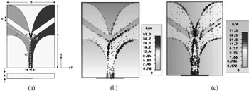
A dual-mode AVA is presented in [Reference Natarajan, Kanagasabai and Gulam Nabi Alsath72]. In this design, the antenna operates in wideband and narrowband modes, as shown in Fig. 27, which operates in the UWB spectrum. In this design, a rectangular strip is etched on the radiator by rotating 45° in the counter clockwise direction to achieve narrowband operation. For performing the wideband operation, switches (S 1, S 2) are placed along the tapered side of the antenna to bridge the slot line. When both the switches are in OFF condition, then the antenna performs the narrowband operation, and when both are in ON condition, then the antenna performs the wideband function. The surface current distributions for narrowband and wideband modes are given in Figs 27(b) and 27(c), respectively, to understand the working of the antenna.
(a) Dual polarized antipodal Vivaldi antenna with W × L × h = 80×60 × 1.6 mm3. (b) Narrowband current distribution. (c) Wideband current distribution [Reference Natarajan, Kanagasabai and Gulam Nabi Alsath72].

In the narrowband operation, the taper section of the antenna is disconnected due to the slot. So, current flows only through the linear slot. On the other hand, in the wideband operation, current flows along the entire taper section of the antenna. The use of rectangular slots in the antenna design provides wideband rejection and enhances the gain of the antenna. The proposed antenna provides higher gain throughout the bandwidth without compromising the gain and impedance performance of the antenna. Again in [Reference Wu, Zhao, Nie and Liu73], a Vivaldi antenna is presented with a stepped connection structure used between a slot line and tapered patches. Due to the presence of this stepped connection structure, the antenna provides better impedance matching as well as wider bandwidth. The antenna also offers better gain due to this structure. A novel structure to enhance directivity, end-fire radiation, and to reduce the sidelobe radiation is presented in [Reference Gao, Li, Zhang and Guo16]. Here to restrict the field radiation and concentrate the energy in the end-fire direction, coupling patches are introduced in the aperture area of the antenna. In [Reference Yin, Yang, Yu and Gao17], a Vivaldi antenna is presented where the gain of the antenna is enhanced by adding a via-loaded maple leaf shape on the edge of the radiator and ground plane. These maple leaves increase the gain at the upper-frequency band.
In [Reference Natarajan, Gulam Nabi Alsath, Kanagasabai, Bilvam and Meiyalagan18], a three-port Vivaldi antenna is presented for diversified applications for vehicular environment. The given antenna is capable of producing three directional radiation patterns. The lower ECC value and higher directivity gain make the antenna appropriate for automobile applications. Slots with variable capacitors or SRRs are employed to create re-configurable AVA for eliminating unwanted bands in [Reference Fusco74].
Conclusion
Vivaldi antenna is one of the most promising candidates for UWB applications due to its wide bandwidth and featured directive radiation characteristics. A thorough review of all Vivaldi antenna performance improvement methods present in most of the literatures has been cited in this paper. These methods are based on the modification based on the physical geometry of an antenna which results in a change in various antenna parameters like size, gain, front to back ratio, bandwidth, radiation pattern, polarization, and operating frequency range. Each technique is discussed in brief with the help of recent research work to prove the impact of a particular technique on antenna parameters. This review work concludes that Vivaldi antenna performance enhancement methods such as slots, corrugation, fractal shapes, dielectric lens, and BAVA can be used to eliminate the undesirable effect of beam squint and cross-polarization. Similarly, the parasitic patch and dielectric lens should be designed such that it will concentrate maximum radiation in the end-fire direction to increase the gain. Furthermore, the designing and positioning of a unit cell of metamaterial on a Vivaldi antenna to enhance its gain, bandwidth, and return loss should be carefully performed. This paper also presents a study of various applications where Vivaldi antenna is used as a critical element. In keeping with this study, the new researchers will be enlightened with all the Vivaldi Antenna performance enhancement methods. They will aid as a guiding principle and reference to applicably select the method while designing an antenna. Lastly, the author expresses regret to the researcher society if any novel contribution in this field is omitted unwittingly during this study.
 Anindita Bhattacharjee belongs from Agartala, Tripura, India. She received her BE degree in Electronics and Communication Engineering from Tripura Institute of Technology, under Tripura University (Central University), Tripura, India in 2014. She received the M.Tech degree in Electronics and Communication Engineering, from Tripura University (Central University), Tripura, India in 2018. Her research interests include analysis and design of compact antennas for wideband applications, ultra-wideband (UWB) antennas, fractal antennas, Vivaldi antenna, MIMO antenna. She has published a number of peer-reviewed journal papers and conference articles.
 Abhirup Bhawal belongs from Kolkata, West Bengal, India. He received his B.Tech degree in Electronics and Communication Engineering from Birbhum Institute of Engineering and Technology and M.Tech degree in Communication Engineering from Netaji Subhash Engineering College, under the West Bengal University of Technology, Kolkata, West Bengal, India in 2011 and 2014, respectively. He is currently pursuing the Ph.D. degree in the Department of Electronics and Communication Engineering, Tripura University (A Central University), Tripura, India. His research interests include analysis and design of compact antennas for wideband applications, ultra-wideband (UWB) antennas, fractal antennas, Vivaldi antennas as well as antennas having special applications like medical imaging, ground-penetrating RADAR, WiFi, etc. He has published several peer-reviewed journal papers and conference articles. He has worked as an Assistant Professor at the Electronics and Communication Engineering Department of Techno India, India.
 Dr. Anirban Karmakar has completed his Ph.D. degree in Engineering from Jadavpur University, Kolkata, India, in 2015. He has more than 13 years of teaching experience and is currently holding the post of Assistant Professor in the Department of Electronics & Communication Engineering at Tripura University (A Central University), India. He has almost 40 research articles in refereed journals and international conference proceedings. He has served as a reviewer in different international journals. He was awarded the best paper award from different international conferences. He is a Senior Member of IEEE and has organized different workshops in the capacity of a convener and completed various funded projects received from UGC. Currently, four research scholars are pursuing Ph.D. under his guidance. His areas of interest include planar and fractal wideband antennas, Arrays, Circular Polarized Antennas, DRA, etc.
 Dr. Anuradha Saha received the gold medal for securing 1st rank in M.Tech. degree in Mechatronics from the National Institute of Technical Teachers' Training and Research, Kolkata in 2009 and obtained Ph.D. degree in Engineering from Jadavpur University in 2017. She has been working as an Assistant Professor in the Department of Applied Electronics and Instrumentation Engineering since 2008 in Netaji Subhash Engineering College, Kolkata, wherein between she has served as full-time research scholar from 2012 to 2015 at the Department of Electronics and Telecommunication Engineering of Jadavpur University, funded by UGC. She is the author of over 30 publications in top international journals and conference proceedings. Her research interests include Artificial Intelligence, Pattern Recognition, Cognitive Robotics, Human-Computer-Interaction as well as Antennas. She is the reviewer of some renowned journals including IEEE Transactions on Fuzzy Systems, IEEE Transactions on Emerging Topics in Computational Intelligence, IETE Journal of Research, and so on.
 Dr. Diptendu Bhattacharya received the B.E. degree from the National Institute of Technology, Jaipur, Rajasthan, India and M.E.Tel.E. (Computer Engineering) from Jadavpur University, Kolkata, India, in 1988 and 1999 respectively. He is currently an Associate Professor in the Department of Computer Science and Engineering, National Institute of Technology, Agartala, Tripura, India. He completed Ph.D. (Engineering) as a QIP Ph.D. fellow from Jadavpur University, Kolkata in 2016. He is working on Machine Intelligence in Economic Time-series prediction. He shouldered administrative responsibilities like Head of Department of Computer Science and Engineering, in the National Institute of Technology, Agartala. He supervised several B.Tech and M.Tech thesis in his teaching period in NIT, Agartala. Presently he is supervising Ph.D. students in NIT Agartala. He is the author of the book “Time Series Prediction and Business Forecasting: A Machine Intelligence Approach” published by Springer, Intelligent Systems Reference Library. His current research interests include type-2 fuzzy sets, artificial intelligence, computational intelligence, fuzzy time-series and its prediction.