2.1. The equations

In the acoustic, i.e. isentropic realm of a perfect gas that we will consider, we have for pressure $\tilde {p}$, velocity $\tilde {\boldsymbol {v}}$, density $\tilde {\rho }$, entropy $\tilde {s}$ and sound speed $\tilde {c}$:

(2.1)\begin{equation} \left. \begin{gathered} \frac{\textrm{d}\test\nx\:\tilde{\rho}}{\textrm{d} t} = - \tilde{\rho}\boldsymbol{\nabla} \boldsymbol{\cdot}\tilde{\boldsymbol{v}},\quad \tilde{\rho}\frac{\textrm{d}\test\nx\:\tilde{\boldsymbol{v}}}{\textrm{d} t} = -\boldsymbol{\nabla} \tilde{p},\\ \frac{\textrm{d}\test\nx\:\tilde{s}}{\textrm{d} t} = \frac{C_V}{\tilde{p}}\frac{\textrm{d}\test\nx\:\tilde{p}}{\textrm{d} t} - \frac{C_P}{\tilde{\rho}}\frac{\textrm{d}\test\nx\:\tilde{\rho}}{\textrm{d} t} = 0,\quad \tilde{c}^2 = \frac{\gamma \tilde{p}}{\tilde{\rho}},\quad \gamma=\frac{C_P}{C_V}, \end{gathered} \right\} \end{equation}

where $\gamma$, $C_P$ and $C_V$ are gas constants and $\textrm {d}/\textrm {d} t = \partial _t + \boldsymbol {v}\boldsymbol {\cdot }\boldsymbol {\nabla }$ denotes the convective derivative; $C_V$ is the heat capacity at constant volume, $C_P$ is the heat capacity at constant pressure and $\gamma = C_P /C_V$. Under isentropic conditions, entropy $\tilde {s}$ is constant along a streamline. We will assume a bit more, namely, the constant $\tilde {s}=s_{ref}$ is the same for all streamlines, which is homentropic flow. In that case we can integrate the entropy equation to get

(2.2)\begin{equation} C_V \log\tilde{p} - C_P \log\tilde{\rho} = s_{ref} = C_V \log p_{ref} - C_P \log \rho_{ref} \end{equation}

or

(2.3)\begin{equation} \frac{\tilde{p}}{p_{ref}} = \left(\frac{\tilde{\rho}}{\rho_{ref}}\right)^{\gamma}. \end{equation}

When we have a stationary mean flow with unsteady time-harmonic perturbations of frequency $\omega$, given, in the usual complex notation, by

(2.4a–c)\begin{equation} \tilde{\boldsymbol{v}} = \boldsymbol{V} + \textrm{Re}(\boldsymbol{v} \textrm{e}^{\textrm{i}\omega t}), \quad \tilde{p} = P + \textrm{Re}(p \textrm{e}^{\textrm{i}\omega t}), \quad \tilde{\rho} = D + \textrm{Re}(\rho \textrm{e}^{\textrm{i}\omega t}), \end{equation}

and linearise for small amplitude, we obtain for the mean flow

(2.5)\begin{equation} \left. \begin{gathered} \boldsymbol{\nabla} \boldsymbol{\cdot} (D \boldsymbol{V} ) = 0, \quad D (\boldsymbol{V} \boldsymbol{\cdot}\boldsymbol{\nabla}) \boldsymbol{V} = -\boldsymbol{\nabla} P,\\ \frac{P}{p_{ref}} = \left(\frac{D}{\rho_{ref}}\right)^{\gamma}, \quad C^2 = \frac{\gamma P}{D}. \end{gathered} \right\} \end{equation}

The mean flow momentum equation can be integrated along streamlines to yield (Batchelor Reference Batchelor1967) a version of Bernoulli's equation that the total specific enthalpy

(2.6)\begin{equation} \frac{1}{2} |\boldsymbol{V}|^2 + \frac{C^2}{\gamma-1} = \text{constant along a streamline}, \end{equation}

not necessarily the same constant for all streamlines. Another quantity, conserved along streamlines, that will be of interest is the specific vorticity $\varXi /D$, where $\varXi =V_x - U_y$. Take the curl of the mean flow momentum equation and substitute the mass conservation to get, by virtue of the pressure being barotropic (Batchelor Reference Batchelor1967),

(2.7)\begin{equation} \boldsymbol{V} \boldsymbol{\cdot}\boldsymbol{\nabla}\left(\frac{\varXi}{D}\right) = 0. \end{equation}

Finally, the perturbations are described by the equations

(2.8)\begin{equation} \left. \begin{gathered} \textrm{i}\omega\rho + \boldsymbol{\nabla} \boldsymbol{\cdot}(\boldsymbol{V}\rho + \boldsymbol{v} D) = 0,\\ D \left(\textrm{i}\omega + \boldsymbol{V}\boldsymbol{\cdot}\boldsymbol{\nabla}\right) \boldsymbol{v} + D \left(\boldsymbol{v} \boldsymbol{\cdot}\boldsymbol{\nabla}\right) \boldsymbol{V} + \rho (\boldsymbol{V}\boldsymbol{\cdot}\boldsymbol{\nabla}) \boldsymbol{V} = -\boldsymbol{\nabla} p,\\ p = C^2 \rho. \end{gathered} \right\} \end{equation}

Myer's time-averaged acoustic energy equations for inviscid and homentropic flow, with $\varXi$ and $\xi$ the mean and perturbed flow vorticity, are given by (Myers Reference Myers1991; Rienstra & Hirschberg Reference Rienstra and Hirschberg2004)

(2.9a)\begin{gather} \boldsymbol{\nabla} \langle \boldsymbol{I} \rangle = -\langle \mathcal{D} \rangle, \end{gather}

(2.9b)\begin{gather} \langle \boldsymbol{I} \rangle = \tfrac{1}{2} \textrm{Re}\left[(D \boldsymbol{v} + \rho \boldsymbol{V}) \left( \frac{p^{\ast}}{D} + \boldsymbol{V} \boldsymbol{\cdot} \boldsymbol{v}^{\ast} \right)\right] , \end{gather}

(2.9c)\begin{gather} \langle \mathcal{D} \rangle = - \tfrac{1}{2} \textrm{Re}[ \xi D \boldsymbol{V} \boldsymbol{\cdot} (-v^{\ast}, u^{\ast}) + \varXi \rho \boldsymbol{v}^{\ast} \boldsymbol{\cdot} (-V, U)]. \end{gather}

2.2. Non-dimensionalisation

Without further change of notation, we will assume throughout this paper that the problem is made dimensionless: lengths on a typical duct height $a_{ref}$, velocities on a typical sound speed $c_{ref}$, time on $a_{ref}/c_{ref}$, densities on a typical density $\rho _{ref}$ and pressures on $\gamma p_{ref}=\rho _{ref}\,c_{ref}^2$. The dimensionless equations are the same as above, except

(2.10)\begin{equation} \gamma P = D C^2 = D^{\gamma}, \end{equation}

while dimensionless frequency $\omega$ is also known as the Helmholtz number.

2.3. The geometry

The domain of interest, sketched in figure 1, is a 2-D duct $\mathcal {V}$ of slowly varying cross-section $g(X)\leq y \leq h(X)$, where $0<h-g= O(1)$; $X = \varepsilon x$ is a so-called slow variable while $\varepsilon$ is small. At the duct top surface $y=h$ and the bottom surface $y=g$, the gradients

(2.11a,b)\begin{equation} \boldsymbol{\nabla} (y-h) = \boldsymbol{e}_y - \varepsilon \boldsymbol{e}_x h_X, \quad \boldsymbol{\nabla} (y-g) = \boldsymbol{e}_y - \varepsilon \boldsymbol{e}_x g_X, \end{equation}

are vectors normal to the surface, so the outward normals of the top and bottom surface are given by

(2.12)\begin{equation} \left. \begin{gathered} \boldsymbol{n}_h = \frac{\boldsymbol{e}_y - \varepsilon \boldsymbol{e}_x h_X}{\sqrt{1+\varepsilon^2 h_X^2}} = \boldsymbol{e}_y - \varepsilon \boldsymbol{e}_x h_X + O(\varepsilon^2),\\ \boldsymbol{n}_g = -\frac{\boldsymbol{e}_y - \varepsilon \boldsymbol{e}_x g_X}{\sqrt{1+\varepsilon^2 g_X^2}} = -\boldsymbol{e}_y + \varepsilon \boldsymbol{e}_x g_X + O(\varepsilon^2). \end{gathered} \right\} \end{equation}

Evidently, $\boldsymbol {e}_x$ and $\boldsymbol {e}_y$ denote the unit vectors in the $x$ and $y$ directions, the indices $h$ and $g$ refer to the top and bottom walls and the index $X$ to a partial derivative to $X$. Except with $\boldsymbol{e}_y$, the index $y$ will be used to denote a partial derivative to $y$.

Figure 1.

Sketch of geometry: two-dimensional slowly varying duct.

2.4. Boundary conditions

If we denote the mean flow by $\boldsymbol {V} = U \boldsymbol {e}_x + V \boldsymbol {e}_y$, the impermeable duct wall yields the mean flow boundary condition $(\boldsymbol {V}\boldsymbol {\cdot }\boldsymbol {n})=0$, or

(2.13a)\begin{equation} V -\varepsilon g_X U = 0 \quad \text{at}\ y=g \end{equation}

and

(2.13b)\begin{equation} V - \varepsilon h_X U = 0 \quad \text{at}\ y=h. \end{equation}

The mean flow mass flux, given by

(2.14)\begin{equation} \int_g^{h} D U \,\textrm{d} y = \mathcal{F}, \end{equation}

is then independent of $x$, where $\mathcal {F}$ is (after non-dimensionalisation) a constant $O(1)$. The mean flow is assumed to be determined by the slowly varying geometry only.

The acoustic boundary condition of the slowly varying lined wall includes the refraction through the vanishing boundary layer, and is a form of the so-called Ingard–Myers condition (Ingard Reference Ingard1959; Myers Reference Myers1980), given at $y=h$ ($i=h$) and $y=g$ ($i=g$) by

(2.15)\begin{equation} \boldsymbol{v}\boldsymbol{\cdot}\boldsymbol{n}_i = \left( \textrm{i}\omega + \boldsymbol{V} \boldsymbol{\cdot} \boldsymbol{\nabla} - \boldsymbol{n}_i\boldsymbol{\cdot}(\boldsymbol{n}_i\boldsymbol{\cdot}\boldsymbol{\nabla} \boldsymbol{V})\right) \left(\frac{p}{\textrm{i}\omega Z_i}\right). \end{equation}

The impedances may vary slowly with position, so we can write $Z_i = Z_i(X)$. It is important to note that $Z_i$ is only defined along a wall, and only derivatives along wall streamlines have meaning.

3.1. The general case

Since we assumed the mean flow to be determined by the slowly varying geometry only, we write all flow variables as a function of $(X,y;\varepsilon )$, and expand each in a regular Poincaré expansion in powers of $\varepsilon ^2$ (the small parameter that appears in the equations). From elementary order of magnitude considerations it follows that $U= O(1)$, $V= O(\varepsilon )$, $D= O(1)$, $C= O(1)$ and $P= O(1)$. So we have

(3.1)\begin{equation} \left. \begin{gathered} U = U_0 + O(\varepsilon^2), \quad V = \varepsilon V_0 + O(\varepsilon^3), \\ D = D_0 + O(\varepsilon^2), \quad P = P_0 + O(\varepsilon^2), \quad C = C_0 + O(\varepsilon^2), \end{gathered} \right\} \end{equation}

where each term in the expansion is independent of $\varepsilon$. For notational convenience we leave out the $0$ subscript, because higher orders will not be considered.

We substitute these expansions in the conservation equations and collect the terms of like powers of $\varepsilon$. Then we get to leading order

(3.2a)\begin{equation} \left. \begin{gathered} (D U)_{X} + (D V)_{y} = 0, \\ D (U U_{X} + V U_{y}) + P_{X} = 0,\\ P_{y} = 0, \end{gathered} \right\} \end{equation}

with boundary conditions

(3.2b)\begin{equation} V - g_X U = 0 \quad \text{at}\ y=g \quad \text{and} \quad V - h_X U = 0 \quad \text{at}\ y=h. \end{equation}

From $P=P(X)$ is also $D=D(X)$ and $C=C(X)$, and so $P_X = C^2 D_X = D^{\gamma -1} D_X$. From the flux condition (2.14) we find

(3.3)\begin{equation} D(X) = \frac{\mathcal{F}}{\displaystyle\int_g^h U(X,y)\, \textrm{d}y}. \end{equation}

Furthermore, the mass and momentum equations become

(3.4)\begin{equation} \left. \begin{gathered} (D U)_X + D V_{y} = 0, \\ D U U_{X} + D V U_{y} + D^{\gamma-1}D_{X} = 0, \end{gathered} \right\} \end{equation}

of which the last equation can be written as

(3.5)\begin{equation} U \def\nx{}\def\test{}\frac{\partial\test\nx\:}{\partial X}\left(\frac{1}{2} U^2 + \frac{D^{\gamma -1}}{\gamma -1}\right) + V \def\nx{}\def\test{}\frac{\partial\test\nx\:}{\partial y}\left(\frac{1}{2} U^2 + \frac{D^{\gamma -1}}{\gamma -1}\right) = 0. \end{equation}

This again amounts to the approximated Bernoulli's equation (2.6), saying that

(3.6)\begin{equation} \frac{1}{2} U^2 + \frac{D^{\gamma -1}}{\gamma -1} = \text{constant along streamlines}, \end{equation}

for example, the wall streamlines at $y=g$ and $y=h$.

By combining the mass equation and $y$-derivative of the momentum equation, we find the approximated version of (2.7)

(3.7)\begin{equation} U\def\nx{}\def\test{}\frac{\partial\test\nx\:}{\partial X}\left(\frac{U_y}{D}\right) + V\def\nx{}\def\test{}\frac{\partial\test\nx\:}{\partial y}\left(\frac{U_y}{D}\right) = 0, \end{equation}

which means that the specific mean shear

(3.8)\begin{equation} \frac{U_y}{D} = \text{constant along streamlines}. \end{equation}

If we start at (say) $X=X_0$ with a linearly sheared flow, i.e. $U_y=\sigma _0$, then the conserved constant $\lambda =\sigma _0/D(X_0)$ is the same for all $X$ and $y$, and $U_y=\lambda D$ everywhere.

The equation of mass conservation leads to

(3.9)\begin{equation} D V = g_X D U|_{y=g} - \int_g^y (D U)_X \,\textrm{d} y', \end{equation}

which satisfies the boundary condition at $y=g$ (by construction), and at $y=h$ because

(3.10)\begin{equation} D V - h_X D U = - \def\nx{}\def\test{}\frac{\textrm{d}\test\nx\:}{\textrm{d} X} \int_g^h D U\, \textrm{d} y = - \def\nx{}\def\test{}\frac{\textrm{d}\test\nx\:}{\textrm{d} X} \mathcal{F} = 0. \end{equation}

For a potential mean flow the above conditions would be sufficient to define the flow (Rienstra Reference Rienstra2003a). For example, $U$ can only be constant in $y$, and the other variables follow by an algebraic equation to be solved at each position $X$. For the vortical mean flow we have here, we need to define an initial velocity profile $(U,\varepsilon V)$ and integrate numerically (iteratively) along streamlines while using (3.3), (3.6) and (3.9). This is not straightforward. See for example Lloyd & Peake (Reference Lloyd and Peake2013) for the closely related cylindrical version of this problem where use is made of the streamfunction.

3.2. Linearly sheared flow

A numerical evaluation of the mean flow is, however, not always necessary. Hinted at by (3.8) and its following paragraph, it appears that for a velocity profile that is linear in $y$, we can find a solution that avoids a numerical integration and much like the potential flow solution requires no more than solving an algebraic equation. Even more, an accidental property will, rather unexpectedly, give our acoustic solution for this case the bonus of a complete adiabatic invariant.

The type of velocity profile we will consider is to leading order given by

(3.11)\begin{equation} U(X,y) = \tau(X)+\sigma(X) (y-g(X)), \end{equation}

where $\sigma$ and $\tau$ are to be determined from the conditions of fixed mass flux and varying wall normal. Then

(3.12)\begin{equation} D V = g_X D U - (D \tau )_X (y-g) - \tfrac{1}{2}(D\sigma)_X (y - g)^2, \end{equation}

and

(3.13)\begin{align} D \tau \tau_X + D^{\gamma-1}D_X + ( D \sigma_X - D_X \sigma) ( \tau (y-g) + \tfrac{1}{2} \sigma (y-g)^2) = 0. \end{align}

Equation (3.13) is valid for any X and y. Its y-dependence is only through the polynomial $\tau(y - g) + {\frac{1}{2}} \sigma(y - g)^{2}$. This vanishes for $y = g$, but is otherwise non-zero (except for the uninteresting case $\tau = \sigma = 0$, and possibly a single point $y = g - 2\tau/\sigma)$. Therefore (3.13) requires

(3.14)\begin{gather} D \tau \tau_X + D^{\gamma-1}D_X = 0, \end{gather}

(3.15)\begin{gather} D \sigma_X - D_X \sigma =0, \end{gather}

both of which can be integrated straightaway. So $\sigma /D=$ constant, which agrees with (3.8). Altogether, we find that for any physically allowable (e.g. no supersonic pockets) constants $\lambda$ and $E$, a mean flow exists given by

(3.16)\begin{equation} \sigma = \lambda D \end{equation}

and Bernoulli's equation (3.6) along streamline $y=g$:

(3.17)\begin{equation} \frac{1}{2} \tau^2 + \frac{1}{\gamma-1}D^{\gamma-1} = E. \end{equation}

Eliminate $\tau$ from

(3.18)\begin{equation} \int_g^h D U\,\textrm{d} y = D \int_g^h U\,\textrm{d} y = D (h-g) \left(\tau + \tfrac{1}{2} \sigma \left(h-g\right)\right) = \mathcal{F} \end{equation}

to get

(3.19)\begin{equation} \tau = \frac{\mathcal{F}}{D(h-g)} - \frac{1}{2} \sigma (h-g), \end{equation}

by which Bernoulli's equation (3.6) applies along streamline $y = h$, with constant $E+\lambda\mathcal{F}$. Altogether, we have for given geometry h and g and mean flow constants $\lambda$, E and $\mathcal{F}$, the following algebraic equation:

(3.20)\begin{equation} \frac{1}{2} \left(\frac{\mathcal{F}}{D(h-g)} - \frac{1}{2} \lambda D (h-g) \right)^2 + \frac{1}{\gamma-1}D^{\gamma-1} = E, \end{equation}

to be solved per $X$ for $D$. Then we have $\tau$, $\sigma$, $U$ and $C$ like above, from which $V$ follows

(3.21)\begin{equation} V = g_X U + U|_{y=h} \frac{C^2 - \tau U }{C^2-\tau U|_{y=h} } \, \frac{h_X - g_X}{h-g} (y-g). \end{equation}

Note that there is apparently no slowly varying mean flow of linear shear with $\tau (X)\equiv 0$.

4.1. Slowly varying modes

With the mean flow variables expanded to leading order, and after eliminating $\rho =p/C^2$, we have the acoustic equations

(4.1a)\begin{equation} \left. \begin{gathered} \textrm{i}\omega p + U p_x + D C^2 ( u_x + v_y ) = - \varepsilon \left[ C^2\left(\frac{ U}{C^2}\right)_{X} p + C^2 D_X u + (V p)_y \right] + O(\varepsilon^2),\\ D \left(\textrm{i}\omega u + U u_x \right) + D U_y v + p_x = - \varepsilon \left[ - D^{-1} D_X p + D (U_{X} u + V u_y) \right] + O(\varepsilon^2),\\ D \left(\textrm{i}\omega v + U v_x \right) + p_y = - \varepsilon D (Vv)_y + O(\varepsilon^2), \end{gathered} \right\} \end{equation}

and the lined wall boundary condition at $y=h(X)$ and $y=g(X)$, respectively,

(4.1b)\begin{equation} \left. \begin{gathered} v - \varepsilon h_X u = \left( \textrm{i}\omega + U\def\nx{}\def\test{}\frac{\partial\test\nx\:}{\partial x} + \varepsilon V \def\nx{}\def\test{}\frac{\partial\test\nx\:}{\partial y} - \varepsilon V_y + \varepsilon h_X U_y \right)\left(\frac{p}{\textrm{i}\omega Z_h}\right) + O(\varepsilon^2),\\ - (v - \varepsilon g_X u) = \left( \textrm{i}\omega + U\def\nx{}\def\test{}\frac{\partial\test\nx\:}{\partial x} + \varepsilon V \def\nx{}\def\test{}\frac{\partial\test\nx\:}{\partial y} - \varepsilon V_y + \varepsilon g_X U_y \right)\left(\frac{p}{\textrm{i}\omega Z_g}\right) + O(\varepsilon^2). \end{gathered} \right\} \end{equation}

We seek slowly varying modes of the form

(4.2)\begin{equation} [p,u,v] = \left[\varPsi(X,y;\varepsilon), A(X,y;\varepsilon), B(X,y;\varepsilon)\right] \exp\left({-\textrm{i}\,\int^x\,\kappa(\varepsilon z;\varepsilon)\,\textrm{d} z}\right). \end{equation}

Introduce

(4.3a,b)\begin{equation} \varOmega = \frac{\omega - \kappa U}{C}, \quad \varOmega_y = -\frac{\kappa U_y}{C}, \end{equation}

and substitute (4.2) in (4.1) to obtain after some simplifications to $O(\varepsilon ^2)$

(4.4a)\begin{align} \left. \begin{gathered} \varOmega^2 \varPsi - \kappa D \varOmega C A - \textrm{i} D \varOmega C B_y = \textrm{i} \varepsilon \varOmega C \left[ \left(\frac{U \varPsi}{C^2}\right)_{X} + \left(\frac{V\varPsi}{C^2}\right)_{y} + (D A)_X \right] + O(\varepsilon^2),\\ \kappa D\varOmega C A + \textrm{i} D \varOmega_y C B - \kappa^2 \varPsi = \textrm{i}\varepsilon \kappa D \left[ \left(\frac{\varPsi}{D}\right)_{X} + (U A)_X + V A_y \right] + O(\varepsilon^2),\\ \textrm{i} \frac{D C B}{\varOmega} + \frac{\varPsi_y}{\varOmega^2} = - \varepsilon \frac{D}{\varOmega^2} [ U B_X + (V B)_y ] + O(\varepsilon^2), \end{gathered} \right\} \end{align}

and boundary conditions

(4.4b)\begin{align} \left. \begin{gathered} B - \varepsilon h_X A = \left( \textrm{i}\varOmega C + \varepsilon U\def\nx{}\def\test{}\frac{\partial\test\nx\:}{\partial X} + \varepsilon V \def\nx{}\def\test{}\frac{\partial\test\nx\:}{\partial y} - \varepsilon V_y + \varepsilon h_X U_y \right)\left(\frac{\varPsi}{\textrm{i}\omega Z_h}\right) + O(\varepsilon^2),\\ - (B - \varepsilon g_X A) = \left( \textrm{i}\varOmega C + \varepsilon U\def\nx{}\def\test{}\frac{\partial\test\nx\:}{\partial X} + \varepsilon V \def\nx{}\def\test{}\frac{\partial\test\nx\:}{\partial y} - \varepsilon V_y + \varepsilon g_X U_y \right)\left(\frac{\varPsi}{\textrm{i}\omega Z_g}\right) + O(\varepsilon^2). \end{gathered} \right\} \end{align}

If we take the y-derivative of the third equation of (4.4a), multiply this by $\varOmega^2$, and add the result to the sum of the first two equations of (4.4a), we obtain

(4.5) \begin{align} & \varOmega^2 \left(\frac{\varPsi_y}{\varOmega^2}\right)_{y} + \left(\varOmega^2 - \kappa^2\right) \varPsi = \textrm{i} \varepsilon \varOmega^2 \left[ \frac{C}{\varOmega}\left(\frac{U \varPsi}{C^2} + DA\right)_{X} + \frac{\kappa D}{\varOmega^2}\left(\frac{\varPsi}{D} + UA \right)_{X}\right.\nonumber\\ &\qquad \quad + \left. \frac{1}{\varOmega C} ( V\varPsi )_y + \frac{\kappa DV}{\varOmega^2} A_y + \textrm{i} D \left(\frac{1}{\varOmega^2} \left[ U B_X + (V B)_y \right]\right)_{y} \right] + O(\varepsilon^2), \end{align}

while

(4.6)\begin{equation} \left. \begin{gathered} A = \frac{\kappa \varPsi}{D\varOmega C} - \frac{U_y \varPsi_y }{D \varOmega^2 C^2} + O(\varepsilon) \\ B = \textrm{i} \frac{\varPsi_y}{D\varOmega C} - \frac{\varepsilon}{\varOmega C} \left[ U \left(\frac{\varPsi_y}{D\varOmega C}\right)_{X} + \left( \frac{V\varPsi_y}{D\varOmega C} \right)_{y} \right] + O(\varepsilon^2). \end{gathered} \right\} \end{equation}

We expand to $O(\varepsilon ^2)$

(4.7a–d)\begin{align} A = A_0 + \varepsilon A_1 + \ldots,\quad B = B_0+\varepsilon B_1 + \ldots,\quad \varPsi = \varPsi_0 + \varepsilon \varPsi_1 + \ldots,\quad \kappa = \kappa_0 +\ldots. \end{align}

There is no need for a $\kappa _1$-term, as $\exp \left (-\textrm {i}\varepsilon \int ^x\kappa _1\,\textrm {d} z\right )$ depends on $X$ only and can be absorbed by $\varPsi$, $A$ and $B$. For notational convenience we retain $\kappa$ in the formulas. To leading-order, equation (4.5) reduces to the Pridmore-Brown eigenvalue equation

(4.8a)\begin{equation} \varOmega^2 \left(\frac{\varPsi_{0y}}{\varOmega^2}\right)_{y} + (\varOmega^2 -\kappa^2) \varPsi_0 = 0, \end{equation}

with boundary conditions

(4.8b)\begin{equation} \varPsi_{0y} = \frac{D \varOmega^2 C^2}{\textrm{i}\omega Z_h} \varPsi_0, \qquad \varPsi_{0y} = - \frac{D\varOmega^2 C^2}{\textrm{i}\omega Z_g} \varPsi_0, \end{equation}

where $\varPsi _0$ and $\kappa$ are to be determined. Through $g$, $h$, $U$, $C$, $Z_g$ and $Z_h$, $\varPsi _0$ and $\kappa$ will vary in $X$. Since the equation and boundary conditions are linear and homogeneous, $\varPsi _0$ is only determined up to a slowly varying amplitude. In the following we will derive an adiabatic invariant for $\varPsi _0$ to determine this slowly varying factor.

4.2. Final solution part 1: the general case

The next order of the expanded equation (4.5) is the inhomogeneous Pridmore-Brown equation in $\varPsi _1$:

(4.9a)\begin{align} & \varOmega^2 \left(\frac{\varPsi_{1y}}{\varOmega^2}\right)_{y} + ( \varOmega^2 -\kappa^2 ) \varPsi_1 = \textrm{i} \varOmega^2 \left[\frac{C}{\varOmega} \left(\left(\kappa + \frac{U\varOmega}{C}\right) \frac{\varPsi_0}{\varOmega C} - \frac{U_y \varPsi_{0y}}{\varOmega^2 C^2}\right)_X +\frac{\kappa^2 V \varPsi_{0y}}{\varOmega^3 C}\right.\nonumber\\ &\qquad\left. + \frac{ \kappa D}{\varOmega^2} \left(\frac{\omega\varPsi_0}{D\varOmega C} - \frac{U U_y \varPsi_{0y}}{D\varOmega^2 C^2}\right)_{X} + \left(\frac{V\varPsi_0}{\varOmega C}-\frac{DU}{\varOmega^2} \left(\frac{\varPsi_{0y}}{D\varOmega C}\right)_{X} - \frac{1}{\varOmega^2 C}\left(\frac{ V \varPsi_{0y}}{ \varOmega}\right)_{y}\right)_{y} \vphantom{\left(\frac{ V \varPsi_{0y}}{ \varOmega}\right)}\right], \end{align}

with boundary conditions (obtained by using the directional derivatives of (4.8b) along wall streamlines)

(4.9b)\begin{align} \left. \begin{gathered} \textrm{i} \left(\varPsi_{1y} - \frac{ D \varOmega^2 C^2}{\textrm{i}\omega Z_h} \varPsi_1\right) = \frac{Z_h DU}{\varPsi_0}\left(\frac{\varPsi_0\varPsi_{0y}}{Z_h D\varOmega C}\right)_{X} + \frac{Z_h DV}{\varPsi_0}\left(\frac{\varPsi_0 \varPsi_{0y}}{Z_h D\varOmega C}\right)_{y} + h_X \kappa \varPsi_0,\\ \textrm{i} \left(\varPsi_{1y} + \frac{ D \varOmega^2 C^2}{\textrm{i}\omega Z_g} \varPsi_1\right) = \frac{Z_g DU}{\varPsi_0}\left(\frac{\varPsi_0\varPsi_{0y}}{Z_g D\varOmega C}\right)_{X} + \frac{Z_g DV}{\varPsi_0}\left(\frac{\varPsi_0 \varPsi_{0y}}{Z_g D\varOmega C}\right)_{y} + g_X \kappa \varPsi_0. \end{gathered} \right\} \end{align}

We do not aim to solve this equation, as it would again involve undetermined homogeneous solutions. Instead, we derive a solvability condition on $\varPsi _0$, required for $\varPsi _1$ to exist. For this, we combine equations (4.8a) and (4.9a) into

(4.10)\begin{equation} \textrm{i} \int_g^h \frac{1}{D \varOmega^2 C^2} \left(\left[\text{equation (4.9a)}\right] \varPsi_0 - \left[\text{equation (4.8a)}\right] \varPsi_1\right) \,\textrm{d} y, \end{equation}

then use the self-adjointness of the Pridmore-Brown equation to eliminate $\varPsi _1$ and apply the boundary conditions (4.9b) to obtain

(4.11) \begin{align} & \left[\frac{ZU}{\varOmega^2 C^2}\left(\frac{\varPsi_0 \varPsi_{0y}}{ZD\varOmega C}\right)_{X} + \frac{ZV}{\varOmega^2 C^2}\left(\frac{\varPsi_0 \varPsi_{0y}}{ZD\varOmega C}\right)_{y} + \frac{V\kappa \varPsi_0^2}{U D\varOmega^2 C^2} \right]_g^h \nonumber\\ &\quad =- \int_g^h \frac{\varPsi_0}{DC^2}\left[\vphantom{\left(\frac{V \varPsi_{0y}}{\varOmega}\right)} \frac{C}{\varOmega}\left(\left(\kappa+\frac{U\varOmega}{C}\right)\frac{\varPsi_0}{\varOmega C} - \frac{U_y \varPsi_{0y}}{\varOmega^2 C^2}\right)_{X} + \frac{\kappa^2 V}{\varOmega^3 C}\varPsi_{0y}\right.\nonumber\\ &\qquad + \left. \frac{\kappa D}{\varOmega^2}\left(\frac{\omega\varPsi_0}{D\varOmega C} - \frac{U U_y \varPsi_{0y}}{D\varOmega^2 C^2}\right)_{X} + \left(\frac{V\varPsi_0}{\varOmega C} \!-\!\frac{DU}{\varOmega^2}\left(\frac{\varPsi_{0y}}{D\varOmega C}\right)_{X} \!-\! \frac{1}{\varOmega^2 C}\left(\frac{V \varPsi_{0y}}{\varOmega}\right)_{y}\right)_{y} \right]\,\textrm{d} y. \end{align}

By several partial integrations, using the defining differential equation and collecting together the $X$-derivative of $(\kappa +U\varOmega /C)\varPsi _0^2/D\varOmega ^2 C^2 - \omega U_y \varPsi _0 \varPsi _{0y}/D\varOmega ^4 C^4$, we obtain after a considerable amount of algebra the equation

(4.12)\begin{align} & \left[\frac{Z\varPsi_{0y}}{D\varOmega^2 C^2\varPsi_0}\left(\frac{U \varPsi_0^2}{Z\varOmega C}\right)_{X} + \frac{Z\varPsi_{0y}}{D\varOmega^2 C^2\varPsi_0}\frac{V}{U}\left(\frac{U \varPsi_0^2}{Z\varOmega C}\right)_{y}\right]^h_g \nonumber\\ &\qquad +\def\nx{}\def\test{}\frac{\textrm{d}\test\nx\:}{\textrm{d} X} \int_g^h \left(\kappa+\frac{U\varOmega}{C}\right)\frac{\varPsi_0^2}{D\varOmega^2 C^2} - \frac{\omega U_y \varPsi_0 \varPsi_{0y}}{D\varOmega^4 C^4}\,\textrm{d} y = \int_g^h \frac{\kappa U\varPsi_0 \varPsi_{0y}}{\varOmega^4 C^4} \left(\frac{U_y}{D}\right)_X\,\textrm{d} y. \end{align}

With boundary conditions (4.8b) this becomes

(4.13a)\begin{align} & \def\nx{}\def\test{}\frac{\textrm{d}\test\nx\:}{\textrm{d} X}\left[ \frac{1}{\textrm{i}\omega Z_h}\left. \frac{U \varPsi_0^2}{\varOmega C}\right|_h + \frac{1}{\textrm{i}\omega Z_g} \left. \frac{U \varPsi_0^2}{\varOmega C}\right|_g + \int_g^h \left(\kappa+\frac{U\varOmega}{C}\right)\frac{\varPsi_0^2}{D\varOmega^2 C^2} - \frac{\omega U_y \varPsi_0 \varPsi_{0y}}{D\varOmega^4 C^4}\,\textrm{d} y \right]\nonumber\\ &\qquad\quad =\int_g^h \frac{\kappa U\varPsi_0 \varPsi_{0y}}{\varOmega^4 C^4} \left(\frac{U_y}{D}\right)_X\, \textrm{d} y. \end{align}

This form is interesting because of its congruence with the acoustic power (see below) in the case of cut-on modes in linearly sheared flow and hard walls. An even more elegant form is found by applying the relation (A 1) of appendix A, with $\mathcal {G} = U/D\varOmega C^3$, and absorbing the boundary terms into the integral, to find

(4.13b)\begin{equation} \def\nx{}\def\test{}\frac{\textrm{d}\test\nx\:}{\textrm{d} X}\left[ \int_g^h \frac{1}{D\varOmega^3 C^3} \left(\omega \kappa \varPsi_0^2 + U \varPsi_{0y}^2 \right) \,\textrm{d} y \right] = \int_g^h \frac{\kappa U\varPsi_0 \varPsi_{0y}}{\varOmega^4 C^4} \left(\frac{U_y}{D}\right)_X \,\textrm{d} y. \end{equation}

If we normalise $\varPsi _0$ to $\bar {\varPsi }_0$ in some smooth way and introduce the slowly varying amplitude $N$ such that $\varPsi _0(X,y) = N(X) \bar {\varPsi }_0(X,y)$, then the equation for $N$

(4.14)\begin{equation} \def\nx{}\def\test{}\frac{\textrm{d}\test\nx\:}{\textrm{d} X} [ N^2 F] = N^2 G, \end{equation}

with

(4.15a,b)\begin{align} F(X) = \int_g^h \frac{1}{D\varOmega^3 C^3} \left(\omega \kappa \bar{\varPsi}_0^2 + U \bar{\varPsi}_{0y}^2 \right) \,\textrm{d} y, \quad G(X) = \int_g^h \frac{\kappa U\bar{\varPsi}_0 \bar{\varPsi}_{0y}}{\varOmega^4 C^4} \left(\frac{U_y}{D}\right)_X \,\textrm{d} y, \end{align}

leads to a form of an incomplete adiabatic invariant

(4.16)\begin{equation} N^2(X) = N^2(0)\frac{F(0)}{F(X)}\exp\left(\int_0^X \frac{G(z)}{F(z)}\,\textrm{d} z\right). \end{equation}

This is similar to Peake & Cooper (Reference Peake and Cooper2001), Cooper & Peake (Reference Cooper and Peake2001), Lloyd & Peake (Reference Lloyd and Peake2013) and Rienstra (Reference Rienstra2016b), although now $F$ and $G$ are independent of $X$-derivatives of $\bar {\varPsi }_0$.

4.3. Final solution part 2: linearly sheared flow

If $(U_y/D)_X=0$, $G(X)=0$ and (4.16) reduces to a complete adiabatic invariant. Since $D$ is independent of $y$, this is the case for a linearly sheared mean flow with the property that $U_y/D =$ a constant. As we found above in (3.16), this is not a restriction. It occurs for any linearly sheared flow that is of slow variation! We have then for a constant $Q_0$:

(4.17)\begin{equation} \int_g^h \frac{1}{D\varOmega^3 C^3} (\omega \kappa \varPsi_0^2 + U \varPsi_{0y}^2 ) \,\textrm{d} y = Q_0. \end{equation}

We do not have to normalise $\varPsi _0$: the adiabatic invariant is the normalisation. The size of $Q_0$ is unimportant in a linear problem, although we can use it to scale the solution conveniently. There is, however, a small reservation. For hard walls we can assume $\varPsi$ to be real, in which case the sign of $Q_0$ relates to the propagation direction and cannot be chosen freely. This is due to the fact that for hard-wall real cut-on modes this invariant is, apart from a factor $\omega /2$, equal to the acoustic power passing a duct cross-section $X = \textrm {constant}$, at least, up to the WKB accuracy. We find for the integral of the time-averaged energy flux $\langle \boldsymbol {I} \rangle$ in the $x$-direction (2.9b) (with hard walls, $U_{yy}=0$, real $\varPsi$ and ignoring subscript $0$)

(4.18)\begin{align} \mathcal{P}(X) &= \int_g^h \frac{1}{2} \textrm{Re}\left[\left(DA + \frac{U\varPsi}{C^2}\right)\left(\frac{\varPsi}{D} + U A\right)^{\ast\,}\right]\,\textrm{d} y + O(\varepsilon)\nonumber\\ & = \frac{1}{2}\int_g^h \left(\frac{\kappa\varPsi}{\varOmega C} -\frac{U_y \varPsi_y}{\varOmega^2 C^2} + \frac{U\varPsi}{C^2}\right)\left(\frac{\varPsi}{D} + \frac{\kappa U \varPsi}{D\varOmega C} - \frac{U U_y \varPsi_y}{D\varOmega^2 C^2}\right)\,\textrm{d} y + O(\varepsilon)\nonumber\\ & = \frac{1}{2}\int_g^h \left[\left(\kappa+\frac{U\varOmega}{C}\right)\frac{\omega \varPsi^2}{D\varOmega^2 C^2} - \frac{\omega^2 U_y \varPsi\varPsi_y}{D\varOmega^4 C^4} + \frac{ U_y}{2DC^4}\left(\frac{U^2 \varPsi_y^2}{\varOmega^4}\right)_{y}\right] \,\textrm{d} y + O(\varepsilon) \nonumber\\ & = \tfrac{1}{2} \omega Q_0 + O(\varepsilon). \end{align}

It is clear that, for $\omega >0$, $Q_0$ must be chosen positive when the mode is right running, and negative when it is left running. Another conclusion we may draw is that, as far as the left-hand side of (4.13) describes the acoustic energy of the mode, it couples with the mean flow, to WKB accuracy, only where the specific shear $U_y/D$ changes in $X$.

The simplicity of (4.13) is elegant not only physically but also mathematically, because no $X$-derivatives of $\varPsi$ and $\varPsi _y$ are required. The existence of an adiabatic invariant is a remarkable result, and perhaps not entirely to be expected (Cooper & Peake Reference Cooper and Peake2001; Peake & Cooper Reference Peake and Cooper2001; Lloyd & Peake Reference Lloyd and Peake2013; Rienstra Reference Rienstra2016b), because in general acoustic energy is not conserved in vortical flow. Although for slowly varying real, hard-wall modes in nearly parallel flow the time-averaged acoustic energy source $\langle \mathcal {D}\rangle$ (2.9c) is $O(\varepsilon )$:

(4.19)\begin{equation} \langle \mathcal{D} \rangle = - \frac{1}{2} \textrm{Re}\left[ \textrm{i} \frac{U U_{yy}}{D\varOmega^3 C^3} \varPsi_y^2 + O(\varepsilon) \right] = 0 + O(\varepsilon), \end{equation}

the acoustic power is not necessarily conserved to $O(\varepsilon )$ because the volume integral of $\mathcal {D}$ over a distance $X = O(1)$ may be $O(\epsilon)\, O(1/\epsilon) = O(1)$, finite.

This completes the leading-order solution of the slowly varying modes. From $\varPsi _0$ the other amplitudes $A_0$ and $B_0$ follow with (4.6).

We end this analysis by checking the consistency of the resulting equation for $\varPsi$ with the corresponding results for the potential flow problem, as considered for three dimensions in Rienstra (Reference Rienstra1999, Reference Rienstra2003a). Without shear, i.e. $U_y=0$, the mean flow is irrotational and can be given by a potential; $U$ and so $\varOmega$ are then functions of $X$ only. If also the sound field is given by a potential $\varPhi$ (no vortical perturbations like vorticity shed from sharp edges), such that

(4.20a–c)\begin{align} A = -\textrm{i} \kappa \varPhi + \varepsilon \varPhi_X, \quad B = \varPhi_y, \quad \varPsi = - \textrm{i} D\varOmega C \varPhi - \varepsilon D(U\varPhi_X + V\varPhi_y) + O(\varepsilon^2), \end{align}

and boundary conditions

(4.21)\begin{align} \left. \begin{gathered} \varPhi_y - \frac{D\varOmega^2 C^2}{\textrm{i}\omega Z_h}\varPhi = - \textrm{i}\varepsilon h_X \kappa \varPhi - \frac{\textrm{i}\varepsilon}{\varPhi}\left[ \left(U\def\nx{}\def\test{}\frac{\partial\test\nx\:}{\partial X}+V\def\nx{}\def\test{}\frac{\partial\test\nx\:}{\partial y}\right)\left(\frac{D\varOmega C \varPhi^2}{\textrm{i}\omega Z_h}\right) + (DU)_X \frac{\varOmega C \varPhi^2}{\textrm{i}\omega Z_h}\right],\\ \varPhi_y + \frac{D\varOmega^2 C^2}{\textrm{i}\omega Z_g}\varPhi = - \textrm{i}\varepsilon g_X \kappa \varPhi + \frac{\textrm{i}\varepsilon}{\varPhi}\left[ \left(U\def\nx{}\def\test{}\frac{\partial\test\nx\:}{\partial X}+V\def\nx{}\def\test{}\frac{\partial\test\nx\:}{\partial y}\right)\left(\frac{D\varOmega C \varPhi^2}{\textrm{i}\omega Z_g}\right) + (DU)_X \frac{\varOmega C \varPhi^2}{\textrm{i}\omega Z_g}\right], \end{gathered} \right\} \end{align}

we find upon substitution into (4.5)

(4.22)\begin{align} \varPhi_{yy} + (\varOmega^2-\kappa^2) \varPhi = \frac{\textrm{i} \varepsilon}{D\varPhi}\left[\def\nx{}\def\test{}\frac{\partial\test\nx\:}{\partial X}\left(\left(\kappa + \frac{U\varOmega}{C}\right)D \varPhi^2\right) + \def\nx{}\def\test{}\frac{\partial\test\nx\:}{\partial y}\left( \frac{V\varOmega}{C} D \varPhi^2\right) \right] + O(\varepsilon^2). \end{align}

After expanding $\varPhi =\varPhi _0 + \varepsilon \varPhi _1 + O(\varepsilon ^2)$, this leads (cf. Rienstra Reference Rienstra1999) by the usual manipulations to the adiabatic invariant

(4.23)\begin{align} & \def\nx{}\def\test{}\frac{\textrm{d}\test\nx\:}{\textrm{d} X}\left[ \left. \frac{D^2 U \varOmega C}{\textrm{i}\omega Z_h}\varPhi_0^2\right|_h + \left.\frac{D^2 U \varOmega C}{\textrm{i}\omega Z_g}\varPhi_0^2\right|_g + \int_g^h \left(\kappa + \frac{U \varOmega}{C}\right) D \varPhi^2_0 \,\textrm{d} y \right]\nonumber\\ &\qquad \quad = \def\nx{}\def\test{}\frac{\textrm{d}\test\nx\:}{\textrm{d} X}\left[ \int_g^h \frac{D}{\varOmega C} \left(\omega\kappa \varPhi_0^2 + U \varPhi_{0y}^2\right) \,\textrm{d} y \right] = 0, \end{align}

which agrees with (4.13a) and (4.13b), respectively, for $U_y = 0$ if we identify $\varPhi _0 = \textrm {i} \varPsi _0/D\varOmega C$.

5.1. Numerical solution of the Pridmore-Brown equation

The heart of a numerical evaluation of the above solution is the solution of the Pridmore-Brown eigenvalue equation in $y$ ((4.8a) and (4.8b)) along a grid of points in $x$. At each $x$, we consider eigenfunction $\varPsi (X,y)$ as a function of $y$ only, and keep $X$ fixed.

A number of methods have been reported in the literature, e.g. Chebyshev spectral collocation methods acting on the vector of linearised Euler equations (Cooper & Peake Reference Cooper and Peake2001; Lloyd & Peake Reference Lloyd and Peake2013), shooting methods (Vilenski & Rienstra Reference Vilenski and Rienstra2007b) and collocation methods (Oppeneer et al. Reference Oppeneer, Rienstra, Lazeroms, Mattheij and Sijtsma2011) acting directly on the Pridmore-Brown equation, each with their own benefits.

We will use here a method, published recently in Rienstra (Reference Rienstra2020), which is a classic Galerkin approach based on a symmetric bilinear form. We rewrite (4.8a) with boundary conditions $\textrm {i}\omega \zeta _h\varPsi '(h)=\varOmega ^2\varPsi '(h)$ and $\textrm {i}\omega \zeta _g \varPsi '(g) = - \varOmega ^2\varPsi (g)$ in weak form, which means that we search for eigenfunction $\varPsi$ and eigenvalue $\kappa$ such that for every test function $w$,

(5.1)\begin{equation} \left. \frac{\varPsi w}{\textrm{i} \omega \zeta_h}\right|_h + \left. \frac{\varPsi w}{\textrm{i} \omega \zeta_g}\right|_g + \int_{g}^{h} - \frac{1}{\varOmega^2} \varPsi' w' + \left(1-\frac{\kappa^2 }{\varOmega^2}\right) \varPsi w \,\textrm{d} y = 0. \end{equation}

The prime indicates a partial derivative with respect to $y$. We assume that $\varOmega \neq 0$ for any $y$ along the integration interval, to avoid the relatively unimportant critical layer solutions, not studied here; see Brambley et al. (Reference Brambley, Rienstra and Darau2012). Here, $\varPsi$ will be suitably normalised and then multiplied by a slowly varying amplitude $N$, determined as indicated above by (4.16) or (4.17).

If we assume that $\varPsi$ can be written as a sum over a function basis $\{ \phi _n\}$ of Chebyshev polynomials,

(5.2)\begin{equation} \varPsi = \sum_{\mu=0}^{\infty} a_{\mu} \phi_{\mu}, \end{equation}

and we use the same basis for the test functions, i.e. $w=\phi _{\nu }$, $\nu =0,1,\ldots$, then (5.1) becomes equivalent with the matrix equation

(5.3)\begin{equation} \boldsymbol{\mathsf{M}}(\kappa) \boldsymbol{a} = 0, \quad \boldsymbol{a} = (a_0, a_1, \ldots)^{\textrm{T}}, \end{equation}

for the doubly infinite symmetric matrix $\boldsymbol{\mathsf{M}}$ with elements

(5.4)\begin{equation} {\mathsf{M}}_{\mu\nu}(\kappa) = \left.\frac{\phi_{\mu} \phi_{\nu}}{\textrm{i} \omega \zeta_h}\right|_h + \left.\frac{\phi_{\mu} \phi_{\nu}}{\textrm{i} \omega \zeta_g}\right|_g + \int_{g}^{h} \left\{ - \frac{1}{\varOmega^2} \phi_{\mu}' \phi_{\nu}' + \left( 1- \frac{\kappa^2}{\varOmega^2} \right)\phi_{\mu} \phi_{\nu} \right\}\,\textrm{d} y. \end{equation}

The $\kappa$-derivative $\boldsymbol{\mathsf{M}}'$ can be expressed in a similar way. The integrals of $\boldsymbol{\mathsf{M}}$ and $\boldsymbol{\mathsf{M}}'$ are evaluated by the Gauss–Legendre method, which is efficient and needs relatively few points for a high accuracy.

The eigenvalue $\kappa$ is determined by a quadratically converging Newton-like iteration. Along the slowly varying duct, each previous $X$-position provides an excellent starting value, making, in general, no more than one iteration necessary. Since we deal with one mode, it is no loss of efficiency to find one eigenvalue at a time.

By using the same Gauss–Legendre points for integral (4.13) as for the elements of $\boldsymbol{\mathsf{M}}$ and $\boldsymbol{\mathsf{M}}'$, we can normalise the found solutions as required. Here, we will take the transmitted power at the left entrance of the duct equal to $\mathcal {P}=1$ for right-running modes and at the right entrance equal to $\mathcal {P}=-1$ for left-running modes. Note that the normalisation is on $\varPsi ^2$, rather than $\varPsi$, and we have to select a sign for $\varPsi$ at each $x$-position. The correct sign is of course such that $\varPsi$ is continuous in $x$.

The integrals over $\kappa$ and $G/F$ may be constructed by incremental trapezoidal integration.

5.2. A practical example

A typical and relevant example may be a linearly sheared mean flow. Although our results are valid for any mean flow profile (provided the slowly varying mean flow satisfies (3.8)), linear shear is most interesting in two respects. First, the adiabatic invariant is ‘complete’, i.e. really a constant of the problem, and second, the mean flow may be given explicitly, without an integration along the streamlines.

Although a linear profile of a flow with friction is eventually not realistic (a parabolic profile for laminar flow or $1/7$-power profiles for turbulent flow is more likely; Hinze Reference Hinze1972), it is not entirely unphysical. For example, a realisation of the model may be found in the annular duct behind the fan of a modern, high-bypass turbofan engine, which leads a small fraction of the flow into the core of the engine. Since this annular duct is narrow compared to the diameter, a 2-D approximation is valid for axially propagating modes. Moreover, its mean flow is the continuation of the strongly sheared boundary layer along the inner hub of the engine's inlet duct, thus making a linearly sheared profile relevant.

The configuration chosen is as follows. The right-running mean flow is described by the problem parameters

(5.5a–f)\begin{equation} \lambda = 0.5, \quad \gamma = 1.4, \quad D_{in} = 1, \quad \tau_{in} = 0.2, \quad \mathcal{F} = 0.4496, \quad E= 2.52, \end{equation}

and the duct geometry (with inlet at $x=-3$) by

(5.6)\begin{equation} h(x) = 1- \tfrac{1}{8}(1 + \tanh x), \quad g(x) = 0, \quad -3 < x < 3, \end{equation}

giving an estimated $\varepsilon \simeq 0.1$. See figure 2 for the $U$ and $V$ components. The decreasing duct height results in an increase of $U$ with a slight decrease of $U_y=\sigma$; $V$ is obviously at its maximum near $x=0$ at the upper wall.

Figure 2.

Mean flow in $x,y$-domain. $(a)$ Mean flow $U$. $(b)$ Mean flow $V$.

For the acoustic part we consider a hard-wall and a soft-wall configuration, both with $\omega =15$. The hard-wall case has in total $10$ cut-on modes: $p_1, \ldots , p_5$ right running and $p_{-1}, \ldots , p_{-5}$ left running. The modes $p_6$ and $p_{-6}$ start cut-on at $x=-3$ but become cut-off near $x=-0.055$, where $F(X)=0$, and the approximate solution breaks down. Since beyond this point the modal energy vanishes, mode $p_6$ has to reflect here into a multiple of $p_{-6}$. For this reason the point is called a turning point. In its neighbourhood a local analysis is required (Rienstra Reference Rienstra2000; Cooper & Peake Reference Cooper and Peake2001). Since we have not included this here, we exclude the modes $p_6$ and $p_{-6}$. For the soft-wall case with $Z_h = Z_g = 1+2\textrm {i}$ we consider the right running $p_2$ and left running $p_{-2}$.

With matrix $\boldsymbol{\mathsf{M}}$ chopped off to just $21\times 21$ ($21$ Chebyshev terms) and for the integrals using only $40$ Gauss–Legendre points we obtain all eigenvalues correct in $11$ digits, as can be estimated by doubling these numbers a few times. We expect the same accuracy for the eigenfunctions. The number of $\kappa$-iterations, using the result of the previous $X$-position as starting value, is typically 1 (depending on the number of $X$-positions; here $2400$). Per $X$ and $400$ plot points in $y$, this takes altogether approximately 0.04 s (Matlab2018, Intel Core i5-4670 CPU @ 3.4 GHz).

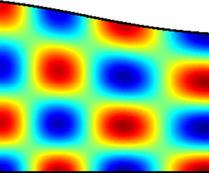
We see that the effects of the sheared mean flow properties are various; see figures 3 and 4 with snapshots of the pressure distribution in the hard-wall duct. For the lowest modal orders, especially upstream running, the asymmetry of the flow is reflected in asymmetric mode shapes. The right-running modes exist only near the lower wall $y=0$ and are negligible at the other side. The upstream-running modes behave the same upside down. This behaviour is due to the sign of $\varOmega ^2-\kappa ^2$: for large enough $\omega$, the mode is oscillatory in $y$ when $\varOmega ^2-\kappa ^2$ is positive, and exponentially decaying otherwise (Rienstra Reference Rienstra2020). For the present, linear, mean flow profile the $y$-interval with oscillatory behaviour is either the full interval, or a part adjacent to the upper or lower duct wall. The contours corresponding to $\varOmega ^2-\kappa ^2=0$ are indicated in the figures by white lines.

Figure 3.

Pressure field snapshots (order $1, \ldots , 5$) for $\omega =15$ and $\mathcal {P} = 1$ (right running). $(a)$ $\kappa _1 = 11.47, \ldots , 9.33$. $(b)$ $\kappa _2 = 9.71, \ldots , 8.27$. $(c)$ $\kappa _3 = 8.77, \ldots , 6.63$. $(d)$ $\kappa _4 = 7.07, \ldots , 3.34$. $(e)$ $\kappa _5 = 4.01, \ldots , -2.26$.

Figure 4.

Pressure field snapshots (order $-1, \ldots , -5$) for $\omega =15$ and $\mathcal {P} = -1$ (left running). $(a)$ $\kappa _{-1} = -43.78, \ldots , -100.04$. $(b)$ $\kappa _{-2} = -32.82, \ldots , -69.40$. $(c)$ $\kappa _{-3} = -26.55, \ldots , -52.84$. $(d)$ $\kappa _{-4} = -22.13, \ldots , -41.69$. $(e)$ $\kappa _{-5} = -19.27, \ldots , -34.44$.

In figures 5 and 6 the mode shapes in $y$ for various $x$ are given in detail. Indeed modes $p_1, p_{-1}, p_{-2}, p_{-3}$, are practically vanishing at the upper, respectively lower, wall. As a result, these modes will not change if the respective wall is lined. Any attenuation due to lining will have to come from the opposite wall. The contours of $\varOmega ^2-\kappa ^2=0$ in the mode shapes figures are given by yellow lines.

Figure 5.

Right-running $n$th-order modal functions $\varPsi _n(X,y)$ for $\omega =15$, as a function of $y-g$ for varying $X$. $\varPsi _6$ becomes cut-off and is not included. $(a)$ $\varPsi _1$. $(b)$ $\varPsi _2$. $(c)$ $\varPsi _3$. $(d)$ $\varPsi _4$. $(e)$ $\varPsi _5$.

Figure 6.

Left-running $n$th-order modal functions $\varPsi _n(X,y)$ for $\omega =15$, as a function of $y-g$ for varying $X$. $\varPsi _{-6}$ becomes cut-off and is not included. $(a)$ $\varPsi _{-1}$. $(b)$ $\varPsi _{-2}$. $(c)$ $\varPsi _{-3}$. $(d)$ $\varPsi _{-4}$. $(e)$ $\varPsi _{-5}$.

The modal wavenumbers $\kappa _n$ as a function of $x$ are given in figure 7. The analogue of the Doppler effect in uniform flow, of increasing wavenumbers for upstream-running modes and decreasing wavenumbers on downstream-running modes, is clearly present.

Figure 7.

Axial wavenumbers $\kappa _1,\ldots , \kappa _{-1}$ (from top to bottom) as a function of $x$. $\kappa _6$ and $\kappa _{-6}$ become cut-off and merge together at $x=-0.055$.

Near $x=0.4$, the value of $\kappa _5$ changes sign, the physical relevance of which is visible in figure 3(e), where the modal wavelength suddenly becomes large, and (this is clearer in an animation) the phase velocity changes from positive to negative. The mode seems to propagate to the right for $x<0.4$ and to the left for $x>0.4$. This, however, is an optical illusion. The energy of the mode remains right-running everywhere.

As the selected impedance does not have much attenuation, the corresponding figures for the lined wall case are comparable. The snap shots of the pressure distribution, figure 8, show the expected Doppler compression upstream and stretching downstream, and the decay to the right for the right-running mode $p_2$ and to the left for the left-running mode $p_{-2}$. We see here and in figure 9 again that the field of $p_{-2}$ practically vanishes near the lower wall.

Figure 8.

Pressure field snapshots (orders ${\pm }2$) for $\omega =15$ and $Z=1+2\textrm {i}$. $(a)$ $\kappa _2 = 9.56-0.84\textrm {i},\ldots , 7.99-0.13\textrm {i}$. $(b)$ $\kappa _{-2} = -30.25+0.38\textrm {i},\ldots , -61.22+0.53\textrm {i}$.

Figure 9.

Real and imaginary parts of modal functions $\varPsi _{{\pm }2}(X,y)$ for $\omega =15$, $Z=1+2\textrm {i}$, as a function of $y-g$ for varying $X$. $(a)$ $\textrm {Re}(\varPsi _{2})$. $(b)$ $\textrm {Im}(\varPsi _{2})$. $(c)$ $\textrm {Re}(\varPsi _{-2})$. $(d)$ $\textrm {Im}(\varPsi _{-2})$.

The attenuation is better displayed by the transmitted power $10 \log _{10}|\mathcal {P}|$ in dB, shown in figure 10. For comparison, the contributions of the exponential, given by $20\log _{10}(\textrm {e}) \,\textrm {Im}\int ^x\kappa _{\pm 2}\,\textrm {d} x'$, has been added as dashed lines. The difference between the exponential and the power is very small (on the logarithmic scale), and the role of the modal shape function in the decay is small here. The lines are not straight because $\kappa _{\pm 2}$ vary with $x$; see figure 11.

Figure 10.

Axial acoustic power $10\log _{10} |\mathcal {P}|$ in dB of right-running mode $2$ and left-running mode $-2$ as a function of $x$.

Figure 11.

Complex axial wavenumbers $\kappa _{{\pm }2}$ varying from $x=-3$ ($\blacksquare$, green) to $x=3$ ($\bullet$, red).