
I. INTRODUCTION
Recent years have witnessed several attempts to build kinetic Monte Carlo (KMC) modelsReference Bortz, Kalos and Lebowitz1–Reference Chatterjee and Vlachos4 of materials that are able to reveal fundamentally novel and unique information about the structure, dynamics, and interactions within these materials over long-time scales.Reference Haldar and Chatterjee5–Reference Clouet, Hin, Gendt, Nastar and Soisson14 An essential step toward building a realistic KMC model of a material involves gaining knowledge of atomistic-scale events that are crucial to the dynamics. We term such events as dynamically relevant events.Reference Bhoutekar, Ghosh, Bhattacharya and Chatterjee15–Reference Bhute and Chatterjee17 One strategy that can be used to accomplish this step entails the use of molecular dynamics (MD) method,Reference Allen and Tildesley18 which has gained significant popularity because of its simplicity. Most research groups around the world possess computational resources that allow for a microsecond long MD simulations of nano-sized systems.Reference Shaw, Bowers, Chow, Eastwood, Ierardi, Klepeis, Kuskin, Larson, Lindorff-Larsen, Maragakis, Moraes, Dror, Piana, Shan, Towles, Salmon, Grossman, Mackenzie, Bank, Young, Deneroff and Batson19 It becomes challenging to study the dynamically-relevant events that are rare at the accessible MD timescales. Significant strides have been made in the algorithmic development of rare-event techniques that can overcome these bottlenecks.Reference Laio and Parrinello20–Reference Béland, Brommer, El-Mellouhi, Joly and Mousseau31 Yet several questions remain about the relevance of mechanisms found using these techniques, and whether the complexities arising due to the large number of configurations and kinetic pathways while building KMC models can be handled by the rare-event techniques.
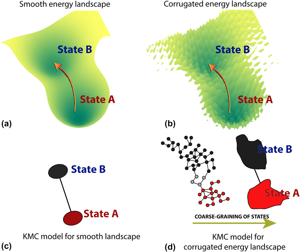
It will be greatly beneficial if the strengths of the MD method, namely, providing exact rate constantsReference Voter32 and sampling of dynamically-relevant events without any prior assumptions about these events,Reference Bhoutekar, Ghosh, Bhattacharya and Chatterjee15–Reference Bhute and Chatterjee17 can be retained as far as possible while addressing the computational cost issue. We review one such rare-event technique called the temperature-programmed molecular dynamics (TPMD)Reference Divi and Chatterjee33,Reference Imandi and Chatterjee34 that possesses these traits. TPMD was originally developed to study thermally-activated events from states lying on corrugated potential energy landscapes.Reference Wales35 Materials characterized by such landscapes typically contain a large number of super states. The system can rapidly interconvert between potential basins lying within the super-state, e.g., states A and B in Fig. 1(b). However, transitions from one super-state to another are rare. This common challenge associated with the study of rare events is called the “low-barrier” problem. The path taken by the system during transitions between the super-states may not be unique and several saddle points may lie along the way. The study of smooth potential energy landscapes with TPMD is also possible.
Unlike many rare-event methods that are geared toward studying smooth energy landscapes (panel a), the TPMD method can also be used for materials with a corrugated energy landscape (panel b) without prior knowledge of the reaction coordinates. Corresponding KMC models constructed using TPMD are shown in panels (c and d).

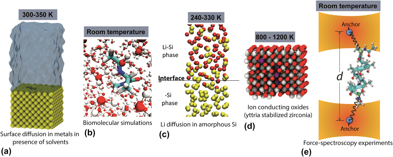
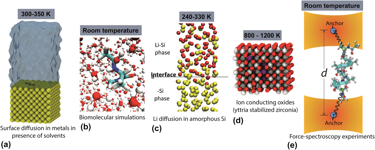
Examples of materials with corrugated potential energy landscapes includes solid–liquid interfaces, where the solvent molecules can rearrange themselves in a number of ways whereas moves involving the solid atoms are rareReference Imandi and Chatterjee34 [Fig. 2(a)]. In biomolecular systems,Reference Chatterjee and Bhattacharya36–Reference Chatterjee and Bhattacharya38 fast-moving solvent molecules and rapid transitions involving some sections of the molecule need to be ignored, whereas the slow transitions are generally of interest [Figs. 2(b) and 2(e)]. Corrugation in the potential energy landscape can be observed as an artifact of the interatomic potential as well as due to the presence of long-range elastic and electrostatic interactions. For instance, lithium transport across the amorphous Li–Si—amorphous Si interface [Fig. 2(c)] is rare, although Li atoms can move rapidly inside the bulk regions.Reference Haldar and Chatterjee39 Similarly, during oxygen ion movement in fast ion conductors,Reference Jaipal and Chatterjee40 a large number of ionic configurations are adopted by the system by the rapidly moving O2− ions [Fig. 2(d)]. To overcome an explosion in a number of states in these materials, it becomes convenient to define states in terms of configurations within a cut-off while ignoring the ionic positions outside the cutoff.Reference Konwar, Bhute and Chatterjee41 The remainder of our discussion pertains to complexities encountered within these types of material systems and how TPMD can help overcome the underlying complexities.
Examples of some applications of TPMD to materials with an underlying corrugated energy landscape.
II. SETTING THE STAGE: PHILOSOPHY OF THE TPMD METHOD
In TPMD, metastable states (usually corresponding to potential energy basins but not always) are determined using a geometric criterion. The task reduces seeking kinetic pathways from a state and calculating the effective rate constant k. Kinetic pathways are defined only in terms of the initial and final states. Section III contains more discussion on this aspect, whereas Sec. IV addresses the question about for how long or from which state transitions need to be sought before we can probe other states on the energy landscape.
Increasing the temperature is a logical way to gain access to rare-activated events.Reference Sorenson and Voter22 Unfortunately, the use of high temperatures provides hardly any advantage with the frequently encountered low barriers in materials simulations. Instead, significant loss in efficiency can be experienced due to the computational overhead. Thus, MD can be used to seek kinetic pathways when the transitions are frequent. In TPMD, a temperature program is used that raises the MD temperature in stages from low to high temperatures once we realize that the transitions are rare (Sec. III.B). The temperature program is one of the key user-defined parameters for the method. In conjunction, a systematic on-the-fly lumping of metastable states is used to coarse-grain fast transition and focus more on the slower ones. Coarse-graining of states into a super state can be achieved by analyzing the frequency of the observed transitions.Reference Chatterjee and Voter42 As a coarser view is gradually adopted seeking rare kinetic pathways between the states A or B as shown in Fig. 1(b), it becomes more straightforward due to reduction in size of the network model. Thus, a systematic coarse-graining procedure for the states can help in overcoming the low barrier problem. Events that happen at milliseconds timescales and beyond are within reach by using the temperature program.
The TPMD waiting time distribution can be retrieved from the list of observed transitions using the stitching algorithm (Sec. III.D). Thereafter, the effective rate constant at the sampled MD temperatures can be estimated from the waiting time distribution (Sec. III.E). Extrapolating rate constants at high temperatures to lower ones, even when the extrapolated rates have an uncertainty associated with them, provides a useful way of building the KMC model. Assuming that the kinetic rate k associated with the transitions obeys the Arrhenius law, namely,
 $$k = \nu \exp \left( {{{ - E} / {{k_{\rm{B}}}T}}} \right)\quad,$$
where k B is the Boltzmann constant and T is the absolute temperature. Direct estimation of effective pre-exponential factor ν and barrier E from the TPMD waiting time distribution is possible. This can enable prediction of the kinetic rate with the KMC model at several temperatures with an even lower uncertainty (Sec. III.F). Note that Eq. (1) is not a strict requirement for TPMD. Several enhanced sampling methods can efficiently find rare events at a single temperature, but generally calculating rates at multiple temperatures, which is a desirable feature of a KMC model, may end up becoming an arduous task. With TPMD one can estimate rates at separate temperatures using a single calculation. Overview of the coarse-graining procedure in TPMD and advantages of coarse-graining are discussed in Sec. III.G. In case of smooth potential energy landscapes, the TPMD method can also be combined with harmonic TST approaches for rapid estimation of the rate constant in place of statistical estimation of the rate constants and Arrhenius parameters from the waiting time distributions.
Once several kinetic pathways have been discovered questions of completeness of the rate catalog arises. It is possible to prepare a reasonably complete catalog of kinetic mechanisms without any a priori knowledge of these mechanisms. As we shall show, the answer to this question lies in whether all kinetically relevant pathways have been included in the catalog. We present arguments that pertain to uncertainty quantification about inferences gained from the TPMD technique. Rare-event techniques based on MD are naturally well positioned to determine the relevance of kinetic pathways. These aspects are covered in the computational framework described in Sec. IV. Finally, we discuss about challenges that still need to be overcome and future possibilities with the TPMD method in Sec. V. Conclusions are provided in Sec. VI.
III. SEEKING KINETIC PATHWAYS FROM A STATE
Frequently, one builds a kinetic network model wherein the configurational space of the material system under study is partitioned into states [Figs. 1(c) and 1(d)]. The dynamical evolution is approximated in terms of state-to-state transitions by the master equationReference Van Kampen43
 $${{{\rm{d}}{\pi _{\rm{S}}}} \over {{\rm{d}}t}} = \sum\limits_{{\rm{S'}} \ne {\rm{S}}} {{k_{{\rm{S'}} \to {\rm{S}}}}{\pi _{{\rm{S'}}}}\left( t \right)} - \sum\limits_{{\rm{S'}} \ne {\rm{S}}} {{k_{{\rm{S}} \to {\rm{S'}}}}{\pi _{\rm{S}}}\left( t \right)\quad .}$$
Each node in the network denotes a state of the system while the connections between the nodes provide rates of interconversion between the states. TPMD can provide the following kinetic information needed in Eq. (2):
(i) A list of states as well as the connections between the states in the kinetic network model.
(ii) Estimation of kinetic rate constants at different temperatures.
(iii) Testing the appropriateness of the Arrhenius equation.
(iv) On-the-fly coarse-graining of states.
(v) Appropriateness of the kinetic network model in comparison to the true dynamics of the model.
We visit these aspects one-by-one.
A. Detection of transitions from a state
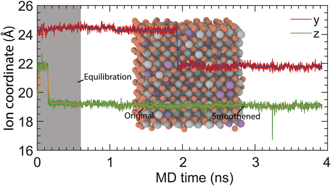
We employ a geometric criterion based on the atomic coordinates to partition the configurational space into states. The system is deemed to be trapped in the same state as long as each atom selected for state identification is at a distance smaller than a chosen tolerance from the configuration representing the state. A transition is said to have occurred when we detect the system has moved to a new metastable state that lies outside the tolerance such that it continues to remain in that state for a stipulated period of time (see Fig. 3). Unless the new state is already present in the state database, a configuration selected after the transition has happened represents the new state of the system. Recrossing events where the system moves to the new state only to quickly return back to the starting state are not counted as transitions (see Fig. 3). One performs MD calculations in state S while checking for a transition at regular intervals. Once a transition is detected, the MD calculation is stopped and the waiting time and final state are noted. This prevents the system from freely diffusing over the potential energy landscape and confines it to a particular state for the purpose of detecting kinetic pathways from the state, calculating the rates and lowering leakage flux of state S. Thus the waiting time distribution collected using TPMD will account for dynamical corrections.
The y- and z-coordinates of an O2− ion in Y2O3-doped ZrO2 (in inset) are shown. A transition is observed at nearly 2 ns along the y-direction. If we allow the MD trajectory to continue a recrossing event is observed at 3.25 ns in the z-direction. Adapted with permission from Ref. Reference Jaipal and Chatterjee40.

In view of the fluctuations in atomic positions, energy minimization techniques have been utilized extensively to identify the metastable states of the system.Reference Divi and Chatterjee33 However, energy minimization calculations are computationally demanding, particularly when a large number of atoms and a large number of snapshots of the material system in the MD trajectory need to be analyzed. An alternative approach involves averaging out the fast vibrational motion of the atoms by employing a Gaussian filterReference Jaipal and Chatterjee40,Reference Deng and Cahill44
 $$w\left( {f,f'} \right) = {c \over {\sqrt {2\pi } \sigma }}\exp \left\{ { - {{{{\left(\, {f' - f} \right)}^2}} \over {2{\sigma ^2}}}} \right\}, - N \le f' \le N\quad ,$$
with N consecutive MD snapshots of the system where c is a normalization constant such that the sum of weights w(f, f′) is one (see Fig. 3). The atomic coordinate in the frame f of the smoothened trajectory is given by
 $${\vec{r}_{{\rm{smooth}}}}\left( f \right) = \sum\limits_{i' = - N}^N {\vec{r}\left( {f + f'} \right)w\left( {f,f'} \right)} \quad .$$
Recrossing events can be eliminated in the smoothened trajectory (see Fig. 3) by proper choice of the filter parameters. The computational cost associated with determining transitions using Eq. (4) is significantly lower than energy-minimization based approach.
B. Temperature program
In TPMD, transitions are sought from a state S using MD trajectories in the canonical ensemble. The MD set-point temperature is specified by a temperature program. The temperature program generally used is given by the form
 $${T_i} = \max \left( {{T_0} + i\Delta T,{T_{\rm{m}}}} \right),i = 0,1,2, \ldots \quad ,$$
so that the temperature is raised in steps over many stages [Fig. 4(a)]. Stage 0 employs the temperature T 0, the set-point temperature at stage i is T i, and ΔT is the uniform temperature increment. Each stage is of a fixed duration τ. T m denotes the maximum allowable high temperature for the system beyond which undesirable effects, such as the state becoming unstable, are introduced.
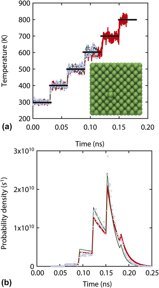
(a) Temperature program used with study of adatom hopping on a metal surface (inset) shown in black line and red lines/white squares show two stochastic realizations with MD trajectories. The consequent acceleration of hopping events as witnessed in terms of the waiting time distribution in panel (b). Comparison between analytical expressions (green line with and red line without anharmonicity correction) and raw waiting time data from TPMD (symbols) is shown. Adapted with permission from Ref. Reference Divi and Chatterjee33.

Transitions are accelerated at higher temperatures where the kinetic rate constant of the large activation barrier events is orders-of-magnitude greater [see Eq. (1)]. For instance, Ag adatom hopping on Ag(100) is observed at millisecond timescales at 300 K, whereas the same kinetic pathways can be witnessed at nanosecond timescales at temperatures greater than 600 K [Fig. 4(b)]. The MD calculation is stopped once a transition from the state is detected. A collection of waiting times from the state can be obtained by repeating the procedure using different random seeds.
A short equilibration step is required at the beginning of each temperature stage such that the system is in thermal equilibrium at all stages. Transitions from the state are not acceptable in the equilibration step. In the event of a transition, the system is returned to the state in question and the equilibration calculation is restarted with a new random seed. The MD time which elapsed the equilibration steps is not included in the waiting time. When multiple TPMD trajectories are generated in parallel using multiple computer processors one employs different random seeds with each trajectory to ensure that all MD calculations are independent. A simpler implementation requires only one thermalization step, namely, before stage 0. Once the initial system is thermally equilibrated, the velocity at the beginning of subsequent temperature stages is obtained by a rescaling algorithm as
 $${v_{i,{\rm{begin}}}} \leftarrow {v_{i - 1,{\rm{end}}}}\sqrt {{{{T_i}} / {{T_{i - 1}}}}} \quad ,$$
such that the velocity of the atoms at beginning of the temperature stage i given by v i,begin can be written in terms of the velocity v i−1,end at the end of the previous temperature stage. Thereafter, the temperature is maintained at the set-point temperature using a Langevin thermostat. Figure 4(a) shows the temperature measured with two different TPMD trajectories in square symbols and red line. The black lines denote the set-point temperature.
C. TPMD waiting time distribution
We are interested in the underlying distribution of waiting times for a particular kinetic pathway α from the state S at the sampled temperatures. Excluding transitions involving other kinetic pathways are discussed as part of the stitching algorithm in Sec. III.D. For constant temperature T 0 MD calculations, the probability p(t)dt associated with α in an infinitesimally small time interval [t, t + dt) is given by
 $$p\left( t \right){\rm{d}}t = \exp \left( { - k_\alpha ^0t} \right)k_\alpha ^0{\rm{d}}t\quad ,$$
here p(t) is the probability density for the waiting time, t is the time elapsed in the state S, and  $k_\alpha ^0$ is the rate constant for α at temperature T 0. Extending Eq. (7) to multiple temperature stages of TPMD, the probability density associated with the transition in stage n is given by
 $$p\left( t \right) = {k_n}\prod\limits_{i = 1}^{{N_{\max }}} {\exp \left( { - {k_i}{\tau _i}} \right)} \quad .$$
The typical shape of the waiting time distribution obtained when only one type of move from the state is present is shown in Fig. 4(b). The probability density is small at early stages when the temperatures are low. An exponential drop in the probability density is observed as we proceed further in each stage. A discontinuous jump in the probability density is observed when the temperature is raised at a new stage. It is likely that the transition would have occurred by the time we reach the later stages, which explains the rapid drop in the probability density. The probability density generally peaks at the intermediate stages when the temperature program parameters have been chosen properly.
From Eq. (8), it becomes evident that the waiting time distribution depends on the kinetic rate at the sampled temperatures. The temperature program plays a role analogous to the potential scan used in electrochemical experimentsReference Bard and Faulkner45 to gain information about the kinetic parameters. Kinetic rates can be recovered using various statistical estimation techniques as described later. Additionally, the effective Arrhenius parameters can be estimated when Arrhenius law [Eq. (1)] is obeyed.
D. Stitching algorithm
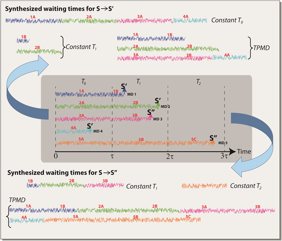
Equation (8) assumes that the waiting time distribution is available for a single kinetic pathway α from the state S, whereas in reality, several pathways could be sampled from the state with TPMD trajectories (Fig. 5). The stitching algorithm enables reducing TPMD data into the form given by Eq. (8). A TPMD trajectory is composed of independent temperature segments, each segment sampling a different temperature, e.g., 1A, 1B for the MD trajectory in Fig. 5. The main idea is to synthesize trajectories by stitching together these independent segments, while ignoring transitions to other states. The stitched trajectory begins in state S and ends in the final state for pathway α. Note that each segment can be utilized at the most one time for a pathway α. The same approach can be used to synthesize trajectories from the same TPMD trajectories for other kinetic pathways from state S. Two types of stitching procedures are useful:
(i) Stitching segments belonging to a constant temperature [waiting time distribution is given by Eq. (7)], and
(ii) Stitching segments belonging to any temperature [waiting time distribution is given by Eq. (8)].
A collection of TPMD trajectories (shown in gray shaded region) from a state S can be mined for waiting times which in turn provides useful kinetic information from the state.

It is instructive to plot the waiting time distribution, e.g., the comparison shown in Fig. 4(b). In particular, one should test the validity of the first-order assumption [Eq. (7)] as well as the Arrhenius approximation in case it is used.
Consider multiple kinetic pathways from state S. Kinetic pathways with larger rate constants are dynamically more relevant since they are selected in the dynamics with a higher probability, i.e., they are required to be present in the KMC model. The probability of selecting higher barrier pathways in the dynamics increases with temperature. Therefore, in many situations the use of lower temperatures at the early stages of the temperature program ensures that the dynamically-relevant pathways will be detected early on while seeking pathways from the state. More number of transitions is observed for low-barrier pathways unless the low-barrier pathways are eliminated via coarse-graining of states (Sec. III.F). This raises an issue, namely, unlike higher-barrier pathways that rate constants for low-barrier pathways are obtained more accurately (see Sec. V for resolution of this issue).
E. Estimation of kinetic rates at sampled temperatures
Once the reactant and product states for the kinetic pathway are known to us one can resort to existing methods including dynamic and molecular-static methods for finding the rate constant for the pathways. For instance, the nudged elastic band methodReference Henkelman, Uberuaga and Jónsson29 alongside the Vineyard equationReference Vineyard46 has been used previously in Ref. Reference Divi and Chatterjee33 for smooth energy landscapes to determine the activation barrier and the pre-exponential factor, respectively. The accuracy of this approach relies on the validity of the harmonic transition state theory (H-TST). Comparisons between the waiting time distribution from TPMD and the predicted H-TST rate can provide an idea of the anharmonicity effect and dynamical corrections for the particular pathway. Figure 4(b) shows the predictions from H-TST (red-line) and the original TPMD distribution (symbols). Adding anharmonicity corrections (green line) provides improved values of the rate constants.
The H-TST approach cannot be used with corrugated energy landscapes. The maximum likelihood analysis provides a convenient procedure for estimating the kinetic rates from waiting time distribution.Reference Pande, Beauchamp and Bowman13 Dynamical corrections are automatically included in the rate estimates. Suppose a collection of m-waiting times  $\left\{ {{{\tilde{t}}_1},{{\tilde{t}}_2}, \ldots,{{\tilde{t}}_m}} \right\}$ is obtained for a particular pathway by stitching segments of the TPMD trajectories at a constant temperature T 0, the likelihood that rate constant has a value k 0 is maximized when the rate constant is given by
 $${k_0} = {m \over {{\theta _0}}}\quad,$$
here  ${\theta _0} = \sum\limits_{i = 1}^m {{{\tilde{t}}_i}}$ is the sum of the waiting times at T 0. Similarly, rate constants are estimated at other temperatures. The availability of a large number of waiting times ensures that the estimate for the rate constant is reliable. One may extrapolate rates calculated at higher temperatures to the lower ones for high barrier pathways. Usually the temperature stage with the fewest number of transitions used for rate extrapolation will contribute most to the uncertainty in the extrapolated rates.
F. Estimation of Arrhenius parameters
One can estimate the Arrhenius parameters using a TPMD dataset simultaneously spanning multiple temperatures (see Fig. 5) in an attempt to lower the uncertainty. Direct estimation of Arrhenius parameters involves solving a nonlinear equation. A collection of m-waiting times {t 1, t 2,…, t m} is obtained for a particular pathway from the stitched TPMD trajectories. Denoting n α as the stage (temperature T nα) where the αth transition happens,  ${\theta _i} = \sum\limits_{\alpha = 1}^m {\tau _i^\alpha }$ is the total time accrued in stage i from the m-waiting times, the value of E a that maximizes the likelihood is obtained by solving
 $${{\sum\limits_{i = 0}^{{N_{\max }}} {{\theta _i}T_i^{ - 1}} \exp \left( { - {{{E_{\rm{a}}}} \over {{k_{\rm{B}}}T}}} \right)} \over {\sum\limits_{i = 0}^{{N_{\max }}} {{\theta _i}\exp \left( { - {{{E_{\rm{a}}}} \over {{k_{\rm{B}}}T}}} \right)} }} = T_{\rm{X}}^{ - 1}\quad,$$
here T X is the harmonic mean temperature, i.e.,  ${T_{\rm{X}}} = {m \over {\sum\limits_{\alpha = 1}^m {T_{{\rm{n}}\alpha }^{ - 1}} }}$. The pre-exponential factor is calculated as
 $$\nu = {m \over {\sum\limits_{i = 0}^{{N_{\max }}} {{\theta _i}\exp \left( { - {{{E_{\rm{a}}}} \over {{k_{\rm{B}}}T}}} \right)} }}\quad .$$
The main advantage of Eq. (10) is that temperature stages that possess large θ-values are expected to contribute most to the determination of the activation barrier.
G. Coarse-graining of states
We shall now focus our attention on coarse-graining of states to avoid the low-barrier problem. Consider the situation in Fig. 6(a) where the states are connected to each other via low barrier moves. Escaping the super-state may either involve high activation barrier moves, e.g., to state S′ or accessing low-probability states such as state x. Fast moves (e.g., the move from state a to b or a to c) can be sampled well using TPMD because of their lower barriers. Gaining knowledge about the slow moves does not serve any purpose at the short timescales as far as the dynamics is concerned. However, when we are interested in the longer timescales slow pathways are of interest.
Systematic on-the-fly coarse-graining procedure allows TPMD to reduce the dimensionality of the kinetic Monte Carlo model in panel (a–c). Panel (d) gives an example of low-barrier problem. Three-adatoms at time 0 ms can rapidly spin at nanosecond timescales as shown in the 12 configurations on the left. On-the-fly coarse-graining helps include the slower kinetic pathways in the KMC model as shown in the dynamical evolution in panel (e). Adapted with permission from Ref. Reference Divi and Chatterjee33.

A large separation of timescales between the slow and fast pathways implies that an equilibrium probability  $\pi _{\rm{S}}^i\left( t \right)$ of residing in state s belonging to the super-state S is quickly attained at the ith temperature stage. The probability is given by
 $$\pi _{\rm{s}}^i = {{\exp \left( { - {{{E_{\rm{s}}}} \over {{k_{\rm{B}}}{T_i}}}} \right)} \over {\sum\limits_{{\rm{s'}}} {\exp \left( { - {{{E_{{\rm{s'}}}}} \over {{k_{\rm{B}}}{T_i}}}} \right)} }}\quad,$$
E s′ is the potential energy of the state s′. Moves within the super-state are ignored while escapes out of the super-state are sought. This is possible by allowing fast moves to happen, but the MD calculation is stopped only once a move out of the super state is detected. The probability density associated with the super-state escape via kinetic pathway α is given by
 $$p\left( t \right) = {\pi _{{\rm{sn}}}}{k_{\rm{n}}}\prod\limits_{i = 1}^{{N_{\max }}} {\exp \left( { - {\pi _{{\rm{s}}i}}{k_i}{\tau _i}} \right)} \quad .$$
An important point to note is that acceleration of rare events happens because of two reasons: better access to (i) low probability states and (ii) high barrier pathways at the high temperatures.
Whether states can be lumped into a super-state is determined on-the-fly on the basis of the superbasin criterion originally developed in Ref. Reference Chatterjee and Voter42. The superbasin criterion requires that a fast move should be observed at least N f times, where
 $${N_{\rm{f}}} = {1 \over \varepsilon }\ln {1 \over \varepsilon }\quad,$$
when the system is trapped in the super-state. The probability for a random-walker to return to a state N f times on a high-dimensional potential energy landscape is less than ε unless it is trapped inside a super-state. The value of ε is decided by the user. For instance, choosing ε = 0.1 yields a value of N f = 23. The super-state definition carries with it the collection of states within it. During the coarse-graining procedure one would add states into the existing list of super-states one-by-one. Figures 6(b) and 6(c) illustrates the growth of the super-state over time. The same approach can be extended to a hierarchy of super-states.
Figure 6(d) shows 12 states involving a Ag adatom trimer that rapidly interconvert at nanosecond timescales. Dissociation events leading to the formation of dimer are rare and happen at millisecond timescales [Fig. 6(e)]. The rare events captured using TPMD demonstrate that the trimer can diffuse on the surface by a series of dissociation and association events. Exchange of atoms with the surface is also possible.
IV. UNCERTAINTY QUANTIFICATION FOR THE RATE CATALOG FROM TPMD
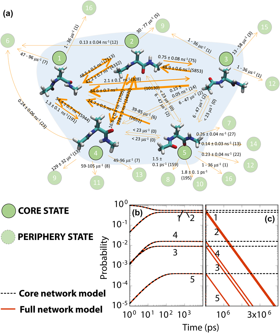
So far we have discussed the use of TPMD calculations in each state to generate of a rate catalog for use with KMC. Figure 7 shows an example of such a procedure used with alanine dipeptide. The kinetic network model was constructed using less than 100 ns MD. The rate constant for the pathways ranges from 1 ns−1 to 10 μs−1. Pathways were sought from only states 1–5 as they were deemed to be important to the dynamics. Although several pathways are sampled using TPMD, the computational effort invested is not enough to establish the maximum duration for which the dynamics is faithfully predicted by the KMC model. For instance, pathways from states 6–16 are missing from the model. In the worst case, missing states and pathways can be important to the dynamics predicted from an “incomplete” KMC model. A conceptual framework that accounts for the missing states/pathways in kinetic network models was discussed in Refs. Reference Haldar and Chatterjee5, Reference Bhute and Chatterjee16, Reference Bhute and Chatterjee17, and Reference Ghosh, Chatterjee and Bhattacharya37.
(a) The KMC model for alanine dipeptide showing the core states. Periphery states are also shown. Predictions from the KMC model at (b) short and (c) long times are shown in dashed lines. Orange lines are predictions from the full network model. Adapted with permission from Ref. Reference Bhoutekar, Ghosh, Bhattacharya and Chatterjee15.

The largest timescale where the KMC model continues to yield the correct dynamics (in comparison to the true dynamics) is termed as the validity time for the model. The true dynamics can be ascertained only via computationally more expensive calculations than the one used to build the KMC model. Therefore, estimates for the validity time are obtained, which forms the main goal of this section. Availability of the validity time allows one to systematically compare the two KMC models of the same system while accounting for known kinetic rates, topology, and relaxation times of the network, as well as missing pathways and states that have not been included in the model. The KMC model can be regarded as complete till its validity time and is safe to use.
A. Core, periphery and missing states
States in Eq. (2) can be partitioned into three types: core, periphery, and missing states. A core state is defined as a state where the system has resided for a significant period of time so that the probability flux out of the state can be estimated with reasonable accuracy from the MD data, i.e., they constitute the source terms in Eq. (2). The KMC model is the core network model, which makes it is ergodic since it is possible to reach a core state from any part of the network, e.g., states 1–5 in Fig. 7. States that are visited for a short time in the TPMD calculation preventing reasonable estimation of kinetic rates from such states are termed as periphery states, e.g., states 6–16 in Fig. 7. Rates from the core states to the periphery states might be available but not the other way around, i.e., periphery states correspond to absorbing or sink states in Eq. (2). Periphery states are redundant at timescales smaller than the KMC validity times but they can become relevant to the dynamics at longer times. A periphery state becomes a core state when sufficient time has been spent in the state. The validity time can be increased by performing additional TPMD in the core and periphery states. States that have never been visited in the MD trajectory are termed as missing states.
B. Calculation of the validity time
Based on these definitions we next construct a network model termed as the full-network model that comprises of core and periphery states as well as contributions from the missing rates. For a core state S, Eq. (2) can be rewritten in terms of the core (C), periphery (P), and missing (M) states as
 $${{{\rm{d}}{\pi _{\rm{S}}}} \over {{\rm{d}}t}} = \sum\limits_{{\rm{S'}} \in {\rm{C}}} {{k_{{\rm{S'}} \to {\rm{S}}}}{\pi _{{\rm{S'}}}}(t)} - \sum\limits_{{\rm{S'}} \in {\rm{C}}} {{k_{{\rm{S}} \to {\rm{S'}}}}{\pi _{\rm{S}}}\left( t \right) - {F_{\rm{S}}}} \quad,$$
where the leakage flux is
 $${F_{\rm{S}}} = \sum\limits_{S' \in {\rm{P}} \cup {\rm{M}}} {\left( {{k_{{\rm{S}} \to {\rm{S'}}}}{\pi _{\rm{S}}} - {k_{{\rm{S'}} \to {\rm{S}}}}{\pi _{{\rm{S'}}}}} \right)} \quad .$$
An upper bound for the missing rates for a core state S is given byReference Bhute and Chatterjee16,Reference Bhute and Chatterjee17
 $$k_{\rm{S}}^{\max } = {{\ln \left( {{1 \over \delta }} \right)} / {{t_{\rm{S}}}}}\quad,$$
here t S denotes the effective TPMD time accrued in the state S at the temperature of interest. In the worst-case scenario, we replace F S with an upper bound by defining the maximum leakage flux from S as
 $$F_{\rm{S}}^{{\rm{leak}}} = k_{\rm{S}}^{{\rm{leak}}}{\hat{\pi }_{\rm{S}}}\quad,$$
where
 $$k_{\rm{S}}^{{\rm{leak}}} = {{\ln \left( {{1 \over \delta }} \right)} \over {{t_{\rm{S}}}}} + \sum\limits_{{\rm{S'}} \in {\rm{P}}} {{k_{{\rm{S}} \to {\rm{S'}}}}} \quad .$$
State occupations for the full network model (denoted by caret) are obtained by solving
 $${{{\rm{d}}{{\hat{\pi }}_{\rm{S}}}} \over {{\rm{d}}t}} = \sum\limits_{{\rm{S'}} \in {\rm{C}}} {{k_{{\rm{S'}} \to {\rm{S}}}}{{\hat{\pi }}_{{\rm{S'}}}}\left( t \right)} - \sum\limits_{{\rm{S'}} \in {\rm{C}}} {{k_{{\rm{S}} \to {\rm{S'}}}}{{\hat{\pi }}_{\rm{S}}}\left( t \right)} - F_{\rm{S}}^{{\rm{leak}}}\quad .$$
The KMC state occupation  ${\tilde{\pi }_{\rm{S}}}\left( t \right)$ is obtained by solving the core-network model
 $${{{\rm{d}}{{\tilde{\pi }}_{\rm{S}}}} \over {{\rm{d}}t}} = \sum\limits_{{\rm{S'}} \in {\rm{C}}} {{k_{{\rm{S'}} \to {\rm{S}}}}{{\tilde{\pi }}_{{\rm{S'}}}}\left( t \right)} - \sum\limits_{{\rm{S'}} \in {\rm{C}}} {{k_{{\rm{S}} \to {\rm{S'}}}}{{\tilde{\pi }}_{\rm{S}}}\left( t \right)} \quad .$$
The validity time for the KMC model is calculated by finding when the state occupations from the core- [Eq. (21)] and full-network models [Eq. (20)] diverge beyond a chosen threshold value [Figs. 7(b) and 7(c)]. Once a state with large leakage is detected, one can analyze the source of leakage and perform additional TPMD calculations accordingly. For instance, additional calculations should be performed in state S when the missing flux from the state is large. On the other hand when the leakage to a periphery state S′ from state S is large one should perform additional TPMD in the periphery state so that it is converted into a core state and its contribution to the leakage is eliminated. Lowering the leakage flux increases the validity time of the KMC model. Enhanced kinetic sampling methods that automatically target states with the largest leakage flux and perform MD calculation in those states are discussed in Ref. Reference Bhoutekar, Ghosh, Bhattacharya and Chatterjee15. The KMC model is thus constructed in patches.
V. FUTURE OUTLOOK
The current version of the TPMD method enables overcoming of several challenges as discussed in this review. To summarize, the main strengths of TPMD include: (i) accelerated sampling of dynamically relevant pathways, (ii) employability with corrugated energy landscapes, (iii) prior knowledge of product configurations/reaction coordinates is not required for KMC model development, (iv) direct estimation of kinetic rates with dynamical and anharmonicity corrections at different temperatures, and if required the Arrhenius parameters, (v) ascertaining the correctness of first-order and Arrhenius assumption, and (vi) uncertainty analysis of the KMC model is possible.
However, there are additional challenges that still need to be overcome. These include:
(i) Lowering the computational cost of TPMD. Since TPMD is based on a dynamical approach it is computationally more expensive than molecular static approaches. The computational efficiency of TPMD is lowered especially due to extremely long waiting times encountered with some trajectories. Major improvements in this regard are required to ensure that TPMD can truly become a method of choice for constructing KMC models for a wide range of materials.
(ii) Enhanced sampling of rare pathways. Since fast pathways are extensively sampled with TPMD, there are fewer transitions involving the slower ones. Although the use of molecular static approaches with TPMD can provide kinetic rates for the slow pathways as described earlier, poor sampling becomes a genuine problem in situations where kinetic rates need to be estimated from waiting time distribution using statistical estimation techniques.
(iii) Tackling the combinatorial complexity arising from a large number of states. The number of states can be restricted to manageable numbers by using local environment descriptions, such as the one introduced in Refs. Reference Jaipal and Chatterjee40 and Reference Konwar, Bhute and Chatterjee41.
(iv) Challenges associated with state and pathway detection. Tolerances used with state definition are ad hoc. In some situations, large fluctuations in atomic coordinates at high temperatures renders the detection of states and pathways slightly challenging.
(v) The effect of variables (temperature, strain, solvent, impurity atoms, etc.) that may influence the kinetic rates associated with these events make the problem truly combinatorial in nature. Cluster expansion models can be used to predict behavior with a large number of environments.Reference Verma, Rehman and Chatterjee47,Reference Rehman, Jaipal and Chatterjee48 However, it is yet to be seen whether the approach can be successfully applied to a wider range of problems.
VI. CONCLUSIONS
In this review, we have concentrated on the theory behind the TPMD method alongside illustration of the method using some applications. The range of applications of the TPMD method continues to grow and we expect to see many new applications of the method in the near future in the areas of rare-event sampling and KMC model development. Of particular interest to the community would be the development of KMC models with error control. This topic is particularly important in the context of present-day KMC models, which are being used increasingly in simulations of complex material systems. In principle, the concepts presented in this review can form the basis for the development of such KMC models. However, it is too early to comment in detail about the algorithmic developments required to overcome the practical challenges that will be faced in this direction.
ACKNOWLEDGMENTS
The author acknowledges support from Science and Engineering Research Board, Department of Science and Technology Grant No. SB/S3/CE/022/2014 and Indian National Science Academy Grant No. SP/YSP/120/2015/307.