Introduction
Luminescence dating of quartz and feldspar minerals is a common Quaternary dating method applied to Pleistocene and Holocene deposits and archaeological features and artifacts (Huntley et al., Reference Huntley, Godfrey-Smith and Thewalt1985; Aitken, Reference Aitken1998). The magnitude of the luminescence signal used for dating is related to three factors; the time since last exposure to heat or light, which resets the luminescence signal (the age of the deposit), the environmental radioactivity of the site (from surrounding sediment and incident cosmic rays), and the sensitivity of the minerals to generate a luminescence signal following absorption of radiation (Murray et al., Reference Murray, Arnold, Buylaert, Guérin, Qin, Singhvi, Smedley and Thomsen2021). Optically stimulated luminescence (OSL) sensitivity is defined as the intensity of the OSL signal emitted (photon counts) for a given radiation dose and sediment mass or volume (Wintle and Murray, Reference Wintle and Murray1999). While OSL sensitivity of quartz is a critical factor for accurate luminescence age determination, the geologic processes that influence quartz OSL sensitivity are still under investigation (Moska and Murray, Reference Moska and Murray2006; Sawakuchi et al., Reference Sawakuchi, Blair, DeWitt, Faleiros, Hyppolito and Guedes2011; Tanski et al., Reference Tanski, Rittenour, Pavano, Pazzaglia, Mills, Corbett and Bierman2024).
OSL sensitivity of quartz is generally weak compared to feldspar and has been shown to be highly variable between settings, deposits, and grains (Duller et al., Reference Duller, Bøtter-Jensen and Murray2000; Sawakuchi et al., Reference Sawakuchi, Rodrigues, Mineli, Mendes, Melo, Chiessi and Giannini2020). The OSL sensitivity of sedimentary quartz is likely initially inherited from its source rock and has been proposed as a potential tool to characterize sediment routing or provenance (Sawakuchi et al., Reference Sawakuchi, Blair, DeWitt, Faleiros, Hyppolito and Guedes2011; Gray et al., Reference Gray, Jain, Sawakuchi, Mahan and Tucker2019; Capaldi et al., Reference Capaldi, Rittenour and Nelson2022; A. Zhang et al., Reference Zhang, Gao, Rahman, Alam, Guo, Chen and Cheng2023; Constantin et al., Reference Constantin, Dave, Grecu, Kabacińska, Antuzevics, Barla, Urdea, Ducea and Timar-Gabor2025). However, recent research also suggests that exposure to surface processes and environmental conditions can further enhance the bedrock OSL sensitivity of quartz (e.g., Pietsch et al., Reference Pietsch, Olley and Nanson2008; Sawakuchi et al., Reference Sawakuchi, Jain, Mineli, Nogueira, Bertassoli, Häggi and Sawakuchi2018; Tanski et al., Reference Tanski, Rittenour, Pavano, Pazzaglia, Mills, Corbett and Bierman2024; Constantin et al., Reference Constantin, Dave, Grecu, Kabacińska, Antuzevics, Barla, Urdea, Ducea and Timar-Gabor2025). Further research into the surface processes that govern OSL sensitivity and modify the original bedrock quartz luminescence characteristics is needed to develop OSL sensitivity as a tool in sediment provenance research.
The goals of this study are to improve understanding of which geologic and Earth-surface processes are responsible for quartz OSL sensitivity by analyzing the OSL sensitivity of modern quartz sand within a small catchment (∼25 km2) with low storage and rapid erosion rates, where we know the sourcing rock type and the modern geomorphic processes. In this context, our dataset from a steep, mountainous catchment, where we expect low OSL sensitivity, provides an opportunity to investigate whether and potentially how quartz OSL can sensitize in an active tectonic setting. We characterize the OSL sensitivity of fluvial sediment from the mainstem, its tributaries, and a single hillslope soil sample. We also measure chemical weathering indices and magnetic susceptibility as proxies for the relative recruitment of soil versus bedrock to the stream alluvium. Finally, we use topographic metrics to test the linkages between fluvial and hillslope processes and OSL sensitivity. By quantifying the catchment’s geomorphic properties within its relatively simple geologic bedrock distribution, we explore potential links between landscape processes and the variability in sensitivity among samples.
OSL sensitivity as a tracer of surface processes
OSL signals are generated from electrons trapped in crystal-lattice defects within quartz that accumulate during exposure to ionizing radiation (Huntley et al., Reference Huntley, Godfrey-Smith and Thewalt1985; Aitken, Reference Aitken1998). OSL sensitivity is related to the number and type of traps (defects), competition among traps, and the probability of charge recombination in luminescence centers (holes) within the mineral grain (Preusser et al., Reference Preusser, Chithambo, Götte, Martini, Ramseyer, Sendezera, Susino and Wintle2009). Traps are understood to be controlled by crystalline defects and impurities like substituting ions, and are related to the geologic conditions of geochemistry, pressure, and temperature during mineral crystallization and subsequent thermal histories (Preusser et al., Reference Preusser, Chithambo, Götte, Martini, Ramseyer, Sendezera, Susino and Wintle2009; Sawakuchi et al., Reference Sawakuchi, Blair, DeWitt, Faleiros, Hyppolito and Guedes2011). This idea that crystallization properties control the number of defects and type suggests that OSL sensitivity can be used as a metric for tracing bedrock provenance of grains, allowing geologists to understand sediment routing and sourcing (Gray et al., Reference Gray, Jain, Sawakuchi, Mahan and Tucker2019; Capaldi et al., Reference Capaldi, Rittenour and Nelson2022; Souza et al., Reference Souza, Pupim, Mazoca, Río, Mineli, Rodrigues, Porat, Hartmann and Sawakuchi2023).
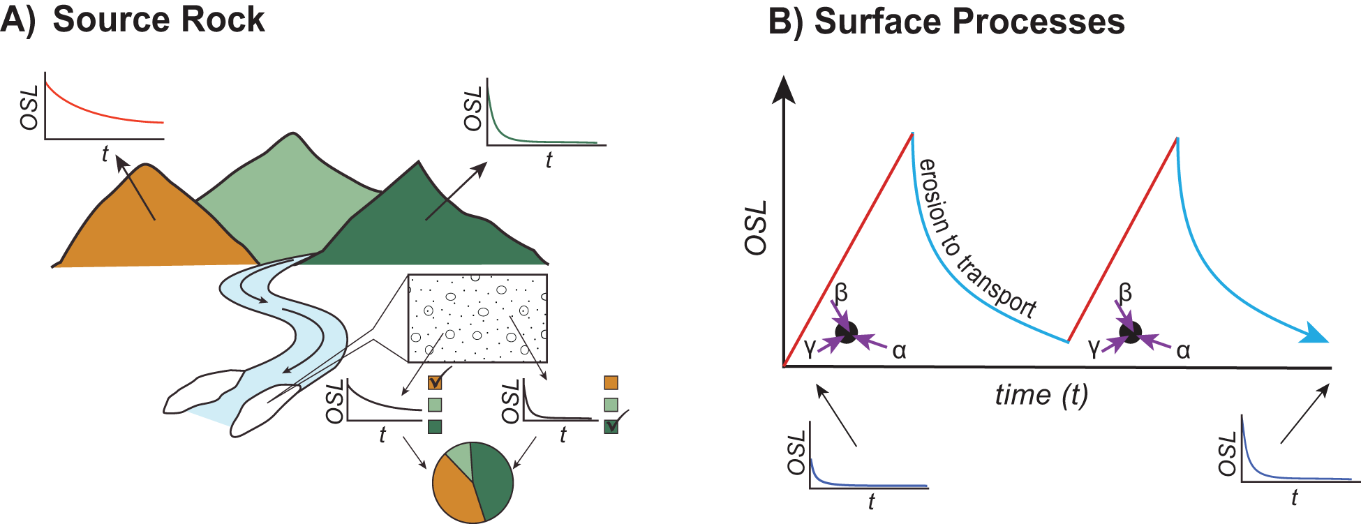
Although quartz OSL sensitivity appears to be inherited from bedrock geologic conditions, many datasets suggest that the sedimentary processes like transport can enhance the original bedrock OSL sensitivity signal. After crystallization, additional defects may develop, and the ratio of luminescent to non-luminescent centers may change in response to exposure to radiation or optical, thermal, or mechanical energy at the Earth’s surface (Aitken, Reference Aitken1998; Preusser et al., Reference Preusser, Chithambo, Götte, Martini, Ramseyer, Sendezera, Susino and Wintle2009; Mineli et al., Reference Mineli, Sawakuchi, Guralnik, Lambert, Jain, Pupim, Rio, Guedes and Nogueira2021). Sawakuchi et al. (Reference Sawakuchi, Blair, DeWitt, Faleiros, Hyppolito and Guedes2011) observed that quartz directly sourced from bedrock has low OSL sensitivity compared with sediment transported by coastal systems. OSL sensitivity has also been documented to increase with downstream distance in some river systems, suggesting that OSL sensitivity can be enhanced by undergoing cycles of exposure to radiation (burial) and bleaching (sunlight) during fluvial transport (Pietsch et al., Reference Pietsch, Olley and Nanson2008; Sawakuchi et al., Reference Sawakuchi, Blair, DeWitt, Faleiros, Hyppolito and Guedes2011; Gliganic et al., Reference Gliganic, Cohen, Meyer and Molenaar2017; Fig. 1B). This pattern is consistent with experiments that have demonstrated an increase in OSL sensitivity following repeated exposures of laboratory irradiation and bleaching (Bøtter-Jensen et al. Reference Bøtter-Jensen, Agersnap Larsen, Mejdahl, Poolton, Morris and McKeever1995; Moska and Murray, Reference Moska and Murray2006; Pietsch et al., Reference Pietsch, Olley and Nanson2008; Constantin et al., Reference Constantin, Dave, Grecu, Kabacińska, Antuzevics, Barla, Urdea, Ducea and Timar-Gabor2025). If exposure to radiation and bleaching cycles lead to quartz OSL sensitization (Fig. 1B), then we would expect that exposure to other surface processes may also enhance the OSL sensitivity. However, some researchers find that OSL sensitivity does not always increase with downstream distance but rather results from changing bedrock source, where additional environmental sensitization is dependent on the crystalline lattice defects during crystallization (Capaldi et al., Reference Capaldi, Rittenour and Nelson2022; A. Zhang et al., Reference Zhang, Gao, Rahman, Alam, Guo, Chen and Cheng2023; Constantin et al., Reference Constantin, Dave, Grecu, Kabacińska, Antuzevics, Barla, Urdea, Ducea and Timar-Gabor2025).
Schematic illustration of how the magnitude of the optically stimulated luminescence (OSL) signal and its decay rate during exposure to light may be influenced by source rock type (A) or enhanced due to exposure to surface processes (B). (A) Illustration of how luminescence properties may be used as a provenance tool (modified from Gray et al., Reference Gray, Jain, Sawakuchi, Mahan and Tucker2019). Each bedrock type has a unique luminescence decay curve. Analysis of the luminescence decay curves from fluvial sediments downstream can be used to understand the relative contributions of each bedrock type. (B) The increase of OSL sensitivity during exposure to cyclic irradiation during burial and bleaching during erosion and transport. The frequency and amplitude of transport cycles, which are influenced by surface processes, may enhance the OSL sensitivity of quartz sand.

Figure 1 Long description
Conceptual scientific schematic labeled A) Source Rock. The left portion shows a landscape with two mountains and a river flowing toward a delta. Small inset plots appear above each mountain, each showing an OSL axis on the vertical and t on the horizontal, with a decay curve descending from left to right. A rectangular inset near the river shows a cross-section of particles. Below the river and delta, two small inset plots appear side by side, each again showing OSL on the vertical axis and t on the horizontal axis, with decay curves. A pie chart appears below these insets, divided into segments corresponding to the mountain types shown above. Conceptual scientific schematic labeled B) Surface Processes. The main graph has a vertical axis labeled OSL and a horizontal axis labeled time left parenthesis t right parenthesis. Two rising and falling cycle shapes are plotted. Each cycle shows a steeply rising straight line followed by a curved descent. A diagonal label reading erosion to transport appears between the rising and falling portions of the first cycle. Near the base of each rising line, a starburst symbol appears with three arrows labeled alpha, beta and gamma pointing toward it. The label beta appears above, gamma to the left and alpha to the right of each starburst symbol. This pattern repeats for the second cycle to the right on the same graph. Below the main graph, two small inset plots appear, one at the lower left and one at the lower right, each showing OSL on the vertical axis and t on the horizontal axis, with a rapid decay curve descending steeply then leveling off.
First-cycle sediments derived from tectonically active mountain ranges typically have low quartz OSL sensitivity and are not dominated by the fast component (e.g., Rhodes, Reference Rhodes2000; Klasen et al., Reference Klasen, Fiebig, Preusser, Reitner and Radtke2007; Palamakumbura et al., Reference Palamakumbura, Robertson, Kinnaird, van Calsteren, Kroon and Tait2016; Ortiz et al., Reference Ortiz, Parra, Rodrigues, Mineli and Sawakuchi2024). In these geologic conditions, where sediments are rapidly eroded and transported, grains are exposed to a limited number of sedimentary cycles. More mature and recycled sediments commonly have increased OSL sensitivity suggesting that exposure to repeated surface processes enhances OSL sensitivity (Sawakuchi et al., Reference Sawakuchi, Blair, DeWitt, Faleiros, Hyppolito and Guedes2011; Ortiz et al., Reference Ortiz, Parra, Rodrigues, Mineli and Sawakuchi2024). In addition, there appears to be an inverse relationship between OSL sensitivity and erosion rates, suggesting that quartz residence time in the critical zone at the surface may enhance OSL sensitivity (e.g. Sawakuchi et al., Reference Sawakuchi, Jain, Mineli, Nogueira, Bertassoli, Häggi and Sawakuchi2018; Dave et al., Reference Dave, Timar-Gabor, Scardia, Safaraliev and Fitzsimmons2022; Souza et al., Reference Souza, Pupim, Mazoca, Río, Mineli, Rodrigues, Porat, Hartmann and Sawakuchi2023; Tanski et al., Reference Tanski, Rittenour, Pavano, Pazzaglia, Mills, Corbett and Bierman2024). However, in situ chemical weathering within weathered saprolite and bedrock does not appear to enhance OSL sensitivity (Cao et al., Reference Cao, Jiang, Xu, Zhao and Zhao2022; Nelson et al., Reference Nelson, Eppes and Rittenour2022). Rather, exposure to other surface processes linked to soil development or mixing, ionizing radiation, hillslope transport or storage, and heat by wildfire has been suggested to enhance OSL sensitivity in some studies (J. Zhang et al., Reference Zhang, Li, Sun, Tongyan, Zhou and Hao2023; Tanski et al., Reference Tanski, Rittenour, Pavano, Pazzaglia, Mills, Corbett and Bierman2024). Keying in on the geomorphic or sedimentary process that leads to the enhancement of OSL sensitivity may improve the utilization of the OSL signal of quartz grains for provenance studies or understanding past geomorphic conditions in sedimentary archives.
Geologic setting of the study area
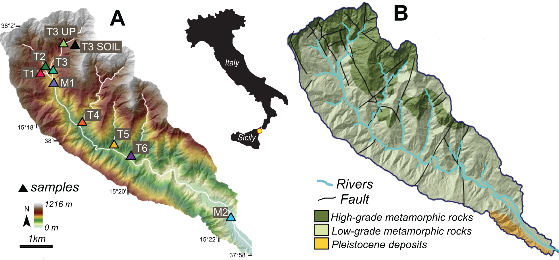
The Pagliara watershed is located in the tectonically active Peloritani Range in northeastern Sicily (Italy) and drains eastward toward the Ionian Sea (central Mediterranean) (Fig. 2). The area is one of the most seismically active regions of the Mediterranean and was struck by catastrophic earthquakes in the past (e.g., M7.1 Messina earthquake in 1908) (Boschi et al., Reference Boschi, Gasperini and Mulargia1995). The Pagliara River has a drainage area of ∼25 km2 and a relief of 1216 m and is underlain by mostly low and lesser amounts of high-grade metamorphic rocks (Fig. 2B). Steep hillslopes and channels result in the watershed acting as an effective conveyor of sediment where rapid rock uplift rates are matched with erosion rates at 1–2 mm/yr (Catalano and De Guidi, Reference Catalano and De Guidi2003; Ferranti et al., Reference Ferranti, Fabrizio Antonioli, Mauz, Amorosi, Dai Pra, Mastronuzzi and Monaco2006; Cyr et al., Reference Cyr, Granger, Olivetti and Molin2010; Pavano et al., Reference Pavano, Pazzaglia, Rittenour, Catalano, Corbett and Bierman2024). The steep headwaters are dominated by landslides (Bucci et al., Reference Bucci, Santangelo, Cardinali, Fiorucci and Guzzetti2016) and debris flows and river channels that coalesce downstream into wide, braided alluvial plains due to the high sediment supply. The localization of intense rainfall events or earthquake-induced surface shaking leads to slope failure and transient sediment pulses that move downstream to the coast (Aronica et al., Reference Aronica, Brigandí and Morey2012; Del Ventisette et al., Reference Del Ventisette, Casagli, Fortuny-Guasch and Tarchi2012; Goswami et al., Reference Goswami, Brocklehurst and Mitchell2012; De Guidi and Scudero, 2013; Ciampalini et al., Reference Ciampalini, Raspini, Bianchini, Frodella, Bardi, Lagomarsino and Di Traglia2015). The catchment has a Mediterranean climate and receives a mean annual precipitation of ∼800 mm (CHELSA dataset from Karger et al., Reference Karger, Conrad, Böhner, Kawohl, Kreft, Soria-Auza, Zimmermann, Linder and Kessler2017). The Pagliara River is ephemeral and commonly does not flow in the summer.
Location maps of the study area. (A) Digital elevation model of the Pagliara watershed with sample locations (triangles). Inset map shows the study location within Sicily, Italy. (B) Geologic map of the Pagliara watershed showing the distribution of low- and high-grade metamorphic rocks (modified from Pavano et al., Reference Pavano, Pazzaglia, Rittenour, Catalano, Corbett and Bierman2024).

Figure 2 Long description
A) The map displays the digital elevation model of the Pagliara watershed with sample locations marked by triangles labeled T1, T2, T3 UP, T3 SOIL, T4, T5, T6, M1 and M2. Elevation ranges from 0 m to 1216 m, with a scale bar indicating 1 km. The inset map shows the location within Sicily, Italy. B) The geologic map illustrates the distribution of high-grade metamorphic rocks, low-grade metamorphic rocks and Pleistocene deposits. Rivers are marked in blue and faults are indicated by black lines. High-grade metamorphic rocks are concentrated in the northern region, while low-grade metamorphic rocks and Pleistocene deposits are more prevalent in the southern areas.
Methods
Sample collection and processing
Ten samples were collected from the Pagliara watershed. Nine samples were from modern river-channel deposits—two from the mainstem (M1, M2) and seven from tributaries (T1, T2, T3, T3 UP, T4, T5, T6)—and one was from modern hillslope soil (T3 SOIL) near the headwaters (Fig. 2A). Each sample was processed to isolate the quartz grains following standard methods (for details, see Tanski et al., Reference Tanski, Rittenour, Pavano, Pazzaglia, Mills, Corbett and Bierman2024). All samples were wet-sieved to isolate the coarsest range of sand used for OSL dating (150–250 µm) to preferentially target fluvially transported sediment and reduce the influence of finer-grained, distally sourced aeolian material. Samples were treated with 3% H2O2 and 30% HCl to remove organic matter and carbonates, respectively, and density separated (2.7 g/cm3) to remove heavy minerals. The samples were etched in 48% HF and 30% HCl to dissolve any feldspar grains, etch the surface of the quartz grains, and prevent fluorite precipitation.
Luminescence measurements
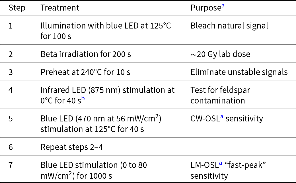
Quartz OSL sensitivity measurements were conducted at Utah State University on a Risø OSL/TL DA-20 instrument with blue-light LED (470 ± 30 nm) and a detection window with 7.5 nm UV filters (U-340) (Bøtter-Jensen et al., Reference Bøtter-Jensen, McKeever and Wintle2003). The sequence procedure is listed in Table 1. Small aliquots (2 mm, ∼80 grains) were mounted on stainless steel disks. The aliquots were first optically bleached to remove the natural signals, given a ∼20 Gy dose using a 90Sr/90Y beta source, and preheated at 240°C to remove unstable signals. This low dose was chosen to ensure OSL sensitivity estimates were derived from the linear portion of the dose–response curve, to reduce the likelihood of saturation effects on the OSL sensitivity calculation, and to provide consistency across samples. The aliquots were tested for feldspar contamination with infrared (IR) stimulation, and aliquots that displayed an IR response (first 0.6 s) greater than three times the background signal (average of the last 3.2 s) were rejected. OSL sensitivity is calculated using the continuous-wave (CW) OSL decay curve, where the luminescence signal is integrated over the first 0.6 s of stimulation with a background subtraction (average of the last 3.2 s). The OSL sensitivity was calculated as the OSL signal response per applied radiation dose and sediment volume on each disk, by estimating sediment volume based on mask size and assuming perfect packing of round grains. Final values are reported as the weighted mean of at least eight small aliquots from each sample. From the CW-OSL curve, we measure the fast ratio, a metric that compares the intensity of the fast decay component relative to the medium and slow components (Durcan and Duller, Reference Durcan and Duller2011). A fast ratio of 20 or greater is usually considered to be fast dominated (Durcan and Duller, Reference Durcan and Duller2011). The linear-modulated OSL (LM-OSL) signal was also measured to determine the relative contribution of the first component (typically considered to be the fast component but could include the medium component) in the LM-OSL decay curve (Bulur et al., Reference Bulur, Bøtter-Jensen and Murray2000). LM-OSL was measured over 1000 s from 0% to 100% LED power (80 mW/cm2) following a ∼20 Gy dose. The LM-OSL curve has an initial peak at 28 s and we measure the first component by integrating the signal over 20–36 s (1.5–3.0 mW/cm2) of stimulation. The LM-OSL sensitivity of the first component is then calculated by subtractintg a background signal measured from blank disks and normalizing by the applied dose and aliquot volume. We report the CW-OSL and LM-OSL sensitivity as the mean and standard error of at least eight aliquots. Additionally, we plot kernel density estimates (KDEs) of each sample to show aliquot variability within a sample.
Optically stimulated luminescence sensitivity sequence procedure.

Table 1 Long description
Columns are Step, Treatment, and Purpose with seven numbered steps. Step 1 is illumination with blue LED at 125 degrees Celsius for 100 seconds, with the purpose, Bleach natural signal. Step 2 is beta irradiation for 200 seconds, with the purpose, approximately 20 gray lab dose. Step 3 is preheat at 240 degrees Celsius for 10 seconds, with the purpose, Eliminate unstable signals. Step 4 is infrared LED stimulation at 875 nanometers at 0 degrees Celsius for 40 seconds with footnote marker b, with the purpose, Test for feldspar contamination. Step 5 is blue LED stimulation at 470 nanometers at 56 milliwatts per square centimeter at 125 degrees Celsius for 40 seconds, with the purpose, continuous wave optically stimulated luminescence sensitivity. Step 6 is repeat steps 2 to 4, and the Purpose cell is blank. Step 7 is blue LED stimulation from 0 to 80 milliwatts per square centimeter for 1000 seconds, with the purpose, linear modulated optically stimulated luminescence fast peak sensitivity.
a CW-OSL, continuous-wave optically stimulated luminescence; LM-OSL, linear-modulated optically stimulated luminescence.
b No heat was added at this step. The sample remained at room temperature (∼25°C).
Topographic metrics
We utilize topographic metrics to compare the geomorphic and evolutionary states of the catchments for each sample. Topographic metrics are extracted using a LIDAR data–derived 2 m digital elevation model (DEM) of the Pagliara watershed (source: Sicily Region–Territory and Environment Department). All topographic metrics were measured using TopoToolbox (Schwanghart and Scherler, Reference Schwanghart and Scherler2014; Forte and Whipple, Reference Forte and Whipple2019).
The fluvial network is extracted to derive the stream longitudinal profile and upstream contributing areas for each sample. We define the fluvial network using an upstream area threshold of 0.25 km2 based on the visual transition of slope to fluvial processes. The slope (S) of a river is defined as a power-law relationship with drainage area (A) known as Flint’s law:
 \begin{equation}S = {k_{\text{S}}}{\text{ }}{A^{ - {{\theta }}}}\end{equation}
where ks is the channel steepness and θ is the channel concavity (Hack, Reference Hack1957; Flint, Reference Flint1974). Channel steepness is normalized (k sn) by a reference concavity (θref) to allow for better comparison between tributary profiles (Wobus et al., Reference Wobus, Tucker and Anderson2006). We use a reference concavity of 0.45 to calculate the mean k sn for each catchment, which is a typical value used for terrain analyses in steady-state, tectonically active channels (Kirby and Whipple, Reference Kirby and Whipple2012) and has been calculated as the mean channel concavity for the Pagliara watershed and the entire Peloritani Range (Pavano et al., Reference Pavano, Pazzaglia and Catalano2016, Reference Pavano, Pazzaglia, Rittenour, Catalano, Corbett and Bierman2024; Pavano, Reference Pavano2025). In addition, for the river-long profile analysis, we applied the integral approach proposed by Perron and Royden (Reference Perron and Royden2013), which allows a horizonal transformation of channel distance (χ), thus linearizing a steady-state channel. For each sub-catchment, channel steepness, which represents the slope of the linearized profile in χ-elevation space, was calculated using the chi-plot TopoToolbox function that finds the concavity that best linearizes the χ-elevation profile (Schwanghart and Scherler, Reference Schwanghart and Scherler2014).
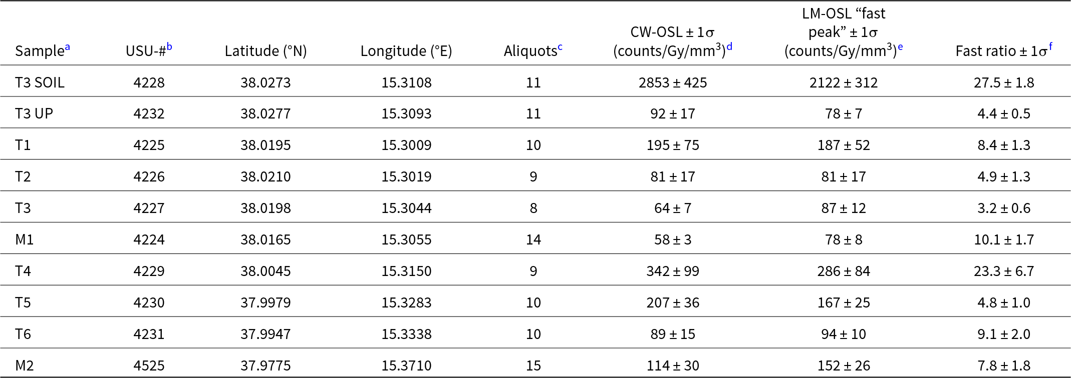
Optically stimulated luminescence (OSL) sensitivity results for samples from the Pagliara watershed.

Table 2 Long description
Ten samples list latitude and longitude, number of aliquots, CW OSL sensitivity and LM OSL fast peak sensitivity in counts per Gy per cubic millimeter, plus a fast ratio. Sample T3 up has CW OSL 92 plus or minus 17, LM OSL fast peak 78 plus or minus 7, and fast ratio 4.4 plus or minus 0.5. Sample T1 has CW OSL 195 plus or minus 75, LM OSL fast peak 187 plus or minus 52, and fast ratio 8.4 plus or minus 1.3. Sample T2 has CW OSL 81 plus or minus 17, LM OSL fast peak 81 plus or minus 17, and fast ratio 4.9 plus or minus 1.3. Sample T3 has CW OSL 64 plus or minus 7, LM OSL fast peak 87 plus or minus 12, and fast ratio 3.2 plus or minus 0.6. Sample M1 has CW OSL 58 plus or minus 3, LM OSL fast peak 78 plus or minus 8, and fast ratio 10.1 plus or minus 1.7. Sample T4 has CW OSL 342 plus or minus 99, LM OSL fast peak 286 plus or minus 84, and fast ratio 23.3 plus or minus 6.7. Sample T5 has CW OSL 207 plus or minus 36, LM OSL fast peak 167 plus or minus 25, and fast ratio 4.8 plus or minus 1.0. Sample T6 has CW OSL 89 plus or minus 15, LM OSL fast peak 94 plus or minus 10, and fast ratio 9.1 plus or minus 2.0. Sample M2 has CW OSL 114 plus or minus 30, LM OSL fast peak 152 plus or minus 26, and fast ratio 7.8 plus or minus 1.8.
a Samples arranged by position from upstream to downstream.
b Utah State University (USU) Luminescence Lab identification number.
c Number of aliquots used to calculate sensitivity.
d Mean of all aliquots. CW-OSL, continuous-wave optically stimulated luminescence.
e Mean of all aliquots. LM-OSL, linear-modulated optically stimulated luminescence.
f Mean of all aliquots. The fast ratio is based on the CW-OSL data.
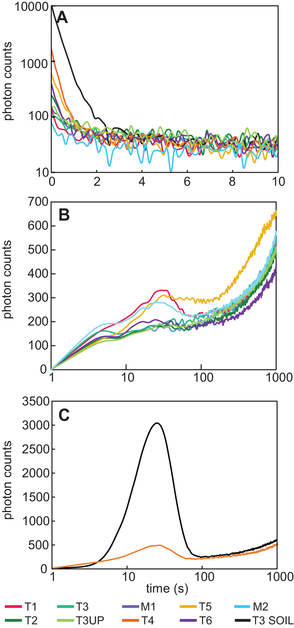
(A) Example continuous-wave optically stimulated luminescence (CW-OSL) curves for all samples from the Pagliara watershed. Averaged linear-modulated OSL (LM-OSL) curves for samples with low OSL sensitivity (B) and samples with high OSL sensitivity (C).

Figure 3 Long description
Panel A: A multi-line graph with the vertical axis labeled photon counts, ranging from 10 to 10000 and the horizontal axis labeled time in seconds, ranging from 0 to 10. The T3 SOIL curve starts near 10000 photon counts and drops steeply, while other curves start between 100 and 2000 photon counts, stabilizing between 20 and 80 photon counts by x equals 2. Panel B: A multi-line graph with the vertical axis labeled photon counts, ranging from 0 to 700 and the horizontal axis labeled time in seconds, ranging from 1 to 1000. Curves rise from near 0 to around 100 to 200 photon counts by x equals 10, with peaks between 250 and 330 photon counts around x equals 20 to 40, then dip and rise again, ending between 400 and 650 photon counts at x equals 1000. Panel C: A two-line graph with the vertical axis labeled photon counts, ranging from 0 to 3500 and the horizontal axis labeled time in seconds, ranging from 1 to 1000. The T3 SOIL curve peaks at about 3000 photon counts between 10 and 30 seconds, while the T4 curve peaks at about 500 photon counts. The legend identifies samples: T1, T2, T3, T3UP, M1, T4, T5, T6, M2, T3 SOIL. The graph demonstrates comparative photon-count dynamics, with T3 SOIL showing distinct behavior.
Hypsometric integral (HI) is a nondimensional metric that quantifies the distribution of elevation within a catchment, offering insight into the geomorphic conditions of the relief within a watershed. The hypsometric integral is here calculated upstream of each sample’s location as elevation-relief ratio, by using Equation 2:
 \begin{equation}{\text{HI}} = \left( {{H_{{\text{mean}}}} - {H_{{\text{min}}}}} \right)/\left( {{H_{{\text{max}}}} - {H_{{\text{min}}}}} \right)\end{equation}
where H mean, H max, and H min, are the mean, maximum, and minimum elevations in the catchment, respectively (Pike and Wilson, Reference Pike and Wilson1971).
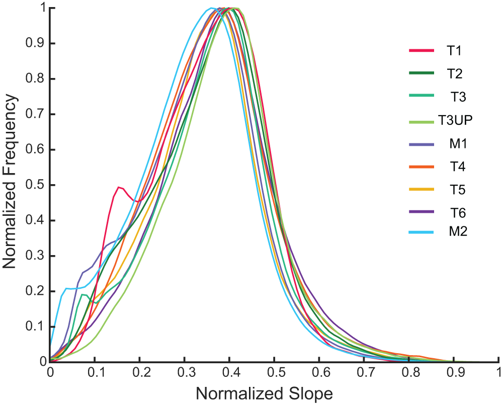
Local relief was calculated from the difference between maximum (H max) and minimum (H min) elevations using a 0.1 km2 moving window; then, for each sub-catchment, we used the mean value of local relief. Aspect was calculated for each catchment and organized into 12° bins. Hillslope gradient was calculated using the elevation change across cells of the DEM using the gradient8 function in TopoToolbox. Frequency distributions of hillslope gradient for each catchment were normalized for comparison between drainages. The hillslope gradient frequency distributions and their relative skewness are used to assess the dominant type of hillslope process (e.g., Wolinsky and Pratson, Reference Wolinsky and Pratson2005).
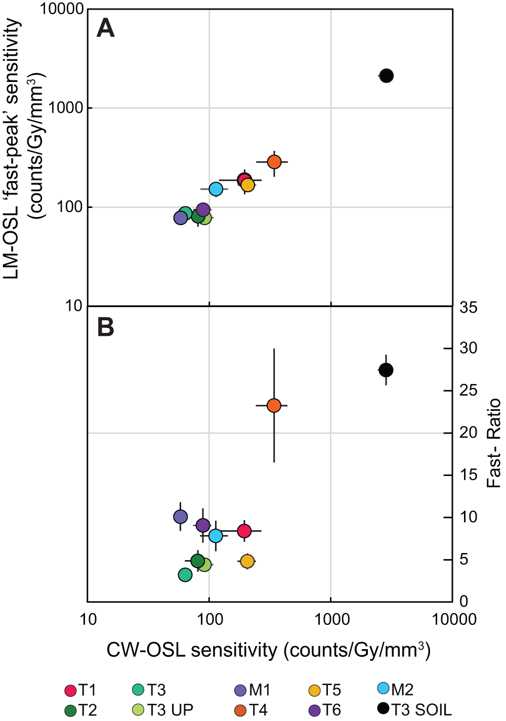
Continuous-wave optically stimulated luminescence (CW-OSL) sensitivity for samples from the Pagliara watershed versus (A) linear-modulated OSL (LM-OSL) “fast-peak” sensitivity and (B) the fast ratio with the gray horizontal line equal to a fast ratio of 20. The sensitivity of the LM-OSL fast peak and the fast ratio are positively related to the CW-OSL sensitivity.

Figure 4 Long description
A showing a scatter plot with the vertical axis label, LM OSL fast peak sensitivity, counts over Gy over millimeter superscript 3, with tick labels 10, 100, 1000, 10000. The horizontal axis uses the same scale as the lower plot, with tick labels 10, 100, 1000, 10000. Points are shown with horizontal and vertical error bars. The plotted points rise as the horizontal axis values increase. A dense group of points lies between approximately 60 and 300 on the horizontal axis and between approximately 70 and 300 on the vertical axis. A single point at approximately 3000 on the horizontal axis and approximately 2000 on the vertical axis is separated from the main group. B showing a scatter plot with the horizontal axis label, CW OSL sensitivity, counts over Gy over millimeter superscript 3, with tick labels 10, 100, 1000, 10000. The vertical axis label is Fast Ratio, with tick labels 0, 5, 10, 15, 20, 25, 30, 35. Points are shown with horizontal and vertical error bars. Most points lie between approximately 60 and 200 on the horizontal axis with fast ratio values between approximately 3 and 10. Two points at higher horizontal axis values are separated from the main group: a point at approximately 300 on the horizontal axis and approximately 23 on the vertical axis and a point at approximately 3000 on the horizontal axis and approximately 28 on the vertical axis. The point at approximately 300 on the horizontal axis and approximately 23 on the vertical axis has a longer vertical error bar spanning roughly from about 17 to about 30. Legend text at the bottom: T1, T2, T3, T3 UP, M1, T4, T5, T6, M2, T3 SOIL.
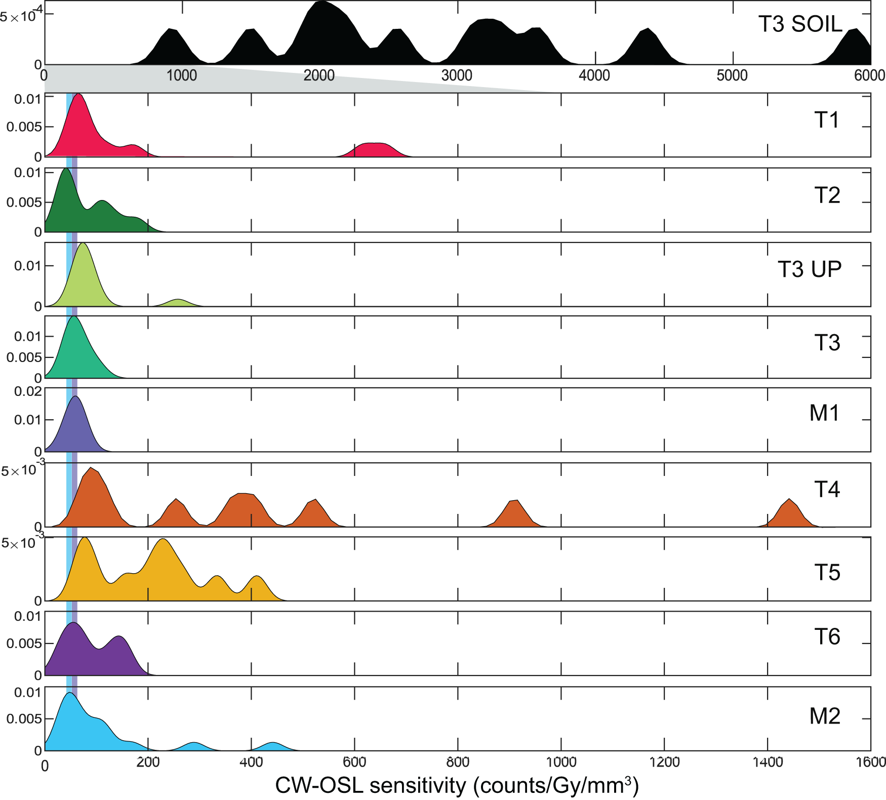
Continuous-wave optically stimulated luminescence (CW-OSL) sensitivity results for samples from the Pagliara watershed as kernel density estimates with a bandwidth of 20 counts/Gy/mm3 for the fluvial samples and 100 counts/Gy/mm3 for the soil sample. Note the change in x-axis for the soil sample relative to the fluvial samples. Blue and purple vertical lines align with the peaks of M2 and M1, respectively, and allow for ease in comparability between sample peaks.

Figure 5 Long description
Ten stacked density plots labeled, T3 SOIL, T1, T2, T3 UP, T3, M1, T4, T5, T6 and M2. Horizontal axis label: CW-OSL sensitivity (counts slash Gy slash mm superscript 3). Horizontal axis tick labels shown on the top plot: 0, 1000, 2000, 3000, 4000, 5000, 6000. Horizontal axis tick labels shown on the bottom plot: 0, 200, 400, 600, 800, 1000, 1200, 1400, 1600. Vertical axis tick labels shown on several plots: 0, 0.005, 0.01. Vertical axis tick labels shown on the T4 and T5 plots: 0 and 5 times 10 superscript 3. Vertical axis tick labels shown on the T3 SOIL plot: 0 and 5 times 10 superscript 4. T3 SOIL: filled density with multiple peaks across the horizontal axis, including peaks near 1000, near 2000, near 3000, near 3500, near 4500 and near 6000. T1: filled density with a main peak near the left side close to 0 and a smaller peak near 600. T2: filled density concentrated near the left side close to 0, with several small peaks between about 0 and 200. T3 UP: filled density with a main peak near the left side close to 0 and a small peak near 250. T3: filled density with a main peak near the left side close to 0. M1: filled density with a main peak near the left side close to 0. T4: filled density with multiple peaks, including peaks near 100, near 250, near 400, near 550, near 900 and near 1450. T5: filled density with multiple peaks between about 0 and 500. T6: filled density with two peaks near the left side, around 50 and around 150. M2: filled density with a main peak near the left side close to 0 and smaller peaks near 250 and near 450.
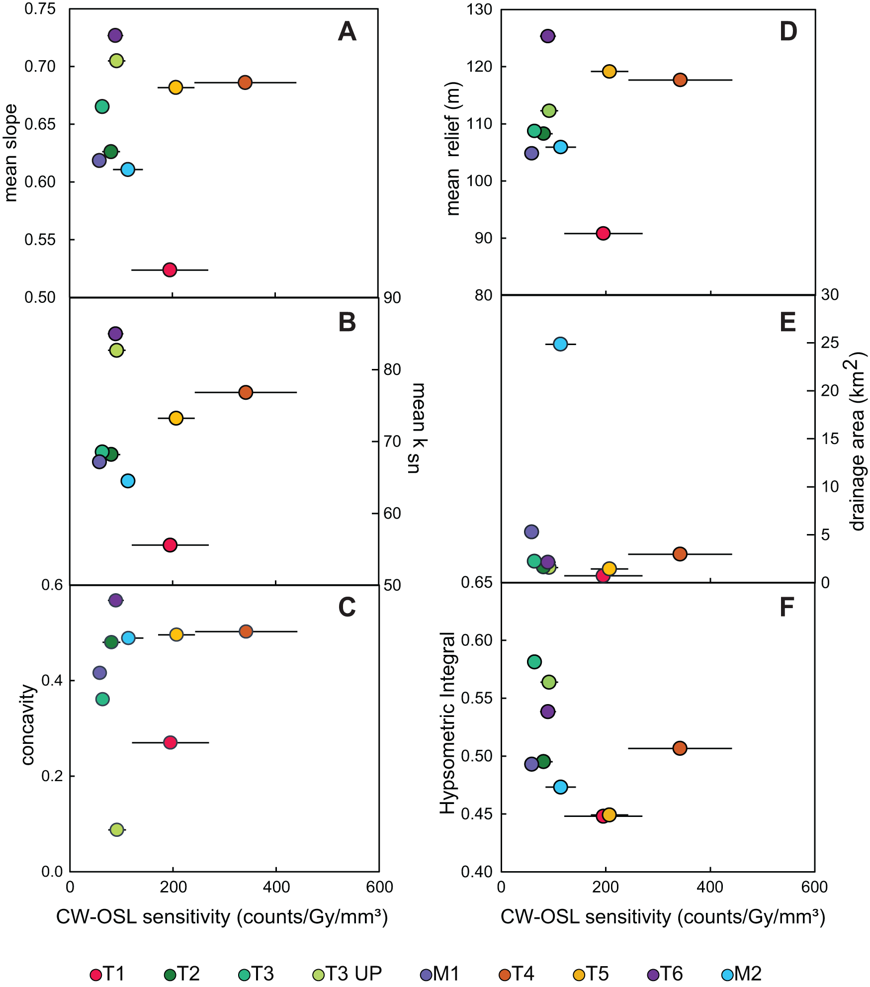
Mean continuous-wave optically stimulated luminescence (CW-OSL) sensitivity ± 1σ versus topographic metrics for samples from the Pagliara watershed: (A) mean slope, (B) mean channel steepness (k sn), (C) concavity, (D) mean relief, (E) drainage area, and (F) hypsometric integral.

Figure 6 Long description
A scatter plot with the horizontal axis labeled, CW OSL sensitivity counts over Gy over mm superscript 3, ranging from 0 to 600. The vertical axis is labeled, mean slope, ranging from 0.50 to 0.75. Points appear near CW OSL sensitivity about 50 to 100 with mean slope about 0.61 to 0.73, one point near about 200 with mean slope about 0.52, one point near about 250 with mean slope about 0.68 and one point near about 350 with mean slope about 0.69. Several points include horizontal error bars. The image B showing a scatter plot with the horizontal axis labeled, CW OSL sensitivity counts over Gy over mm superscript 3, ranging from 0 to 600. The vertical axis is labeled, mean k subscript sn, ranging from 50 to 90. Points appear near CW OSL sensitivity about 50 to 100 with mean k subscript sn about 65 to 85, one point near about 200 with mean k subscript sn about 55, one point near about 250 with mean k subscript sn about 75 and one point near about 350 with mean k subscript sn about 78. Several points include horizontal error bars. The image C showing a scatter plot with the horizontal axis labeled, CW OSL sensitivity counts over Gy over mm superscript 3, ranging from 0 to 600. The vertical axis is labeled, concavity, ranging from 0.0 to 0.6. Points appear near CW OSL sensitivity about 50 to 100 with concavity about 0.35 to 0.58, one point near about 100 with concavity about 0.08, one point near about 200 with concavity about 0.27, one point near about 250 with concavity about 0.50 and one point near about 350 with concavity about 0.50. Several points include horizontal error bars. The image D showing a scatter plot with the horizontal axis labeled, CW OSL sensitivity counts over Gy over mm superscript 3, ranging from 0 to 600. The vertical axis is labeled, mean relief m, ranging from 80 to 130. Points appear near CW OSL sensitivity about 50 to 100 with mean relief about 105 to 125, one point near about 200 with mean relief about 91, one point near about 250 with mean relief about 119 and one point near about 350 with mean relief about 118. Several points include horizontal error bars. The image E showing a scatter plot with the horizontal axis labeled, CW OSL sensitivity counts over Gy over mm superscript 3, ranging from 0 to 600. The vertical axis is labeled, drainage area km superscript 2, ranging from 0 to 30. Points appear near CW OSL sensitivity about 50 to 100 with drainage area about 1 to 6, one point near about 100 with drainage area about 25, one point near about 200 with drainage area about 1 and one point near about 350 with drainage area about 3. Several points include horizontal error bars. The image F showing a scatter plot with the horizontal axis labeled, CW OSL sensitivity counts over Gy over mm superscript 3, ranging from 0 to 600. The vertical axis is labeled, Hypsometric Integral, ranging from 0.40 to 0.65. Points appear near CW OSL sensitivity about 50 to 100 with Hypsometric Integral about 0.47 to 0.58, two points near about 200 with Hypsometric Integral about 0.45 and one point near about 350 with Hypsometric Integral about 0.50. Several points include horizontal error bars. A legend lists T1, T2, T3, T3 UP, M1, T4, T5, T6, M2.
Magnetic susceptibility
Magnetic susceptibility (m3/kg) quantifies the magnetic strength contributed by both ferromagnetic and paramagnetic minerals. A KT-10 handheld susceptibility meter was used in the field to measure the magnetic susceptibility and converted to SI units (m3/kg), assuming a known analysis volume and density of analyzed sample. The presented magnetic susceptibility is the average, and standard deviation as uncertainties, of three replicate measurements. We utilize magnetic susceptibility here as a provenance proxy for the relative recruitment of soils or weathered material relative to non-weathered bedrock, as soil horizons have greater magnetic susceptibility than the underlying parent material, likely due to dust influx and pedogenic production of ferromagnetic minerals (Le Borgne, Reference Le Borgne1955; Maher, Reference Maher1986). In addition, enhancement of magnetic susceptibility in soils has led to its use as a proxy for reconstructing paleoenvironmental conditions (e.g., An et al., Reference An, Kukla, Porter and Xiao1991; Geiss and Zanner, Reference Geiss and Zanner2007; Geiss et al., Reference Geiss, Egli and Zanner2008; Liu and Sun, Reference Liu and Sun2012; Jordanova et al., Reference Jordanova, Jordanova, Mokreva, Ishlyamski and Georgieva2019).
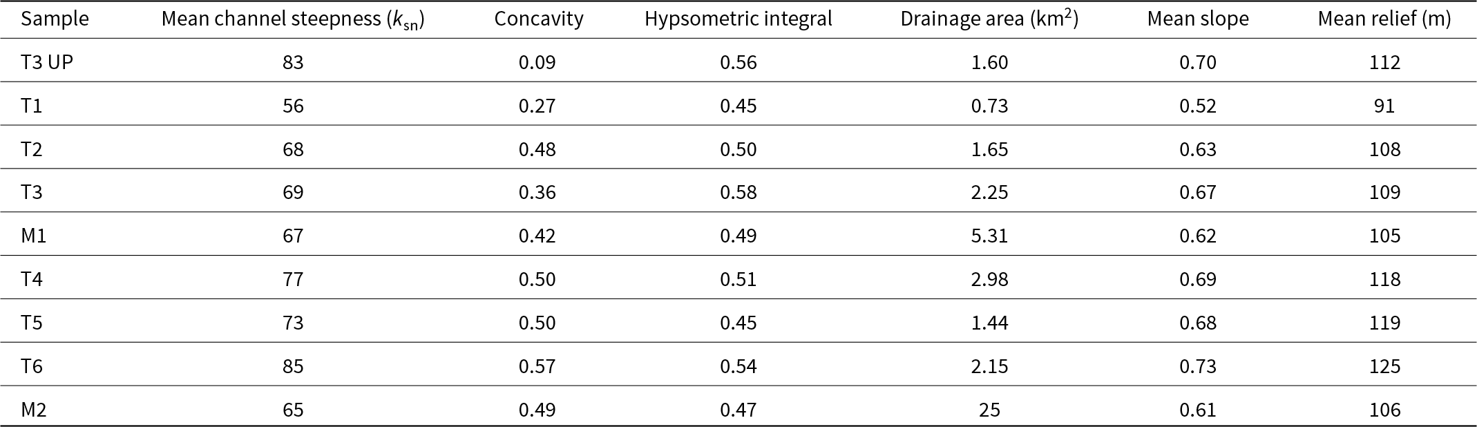
Topographic metrics for fluvial samples from the Pagliara watershed.

Table 3 Long description
Nine samples, T3 UP, T1, T2, T3, M1, T4, T5, T6, and M2, are listed with mean channel steepness, ksn, concavity, hypsometric integral, drainage area in square kilometers, mean slope, and mean relief in meters. T3 UP has ksn 83, concavity 0.09, hypsometric integral 0.56, drainage area 1.60, mean slope 0.70, and mean relief 112. T1 has ksn 56, concavity 0.27, hypsometric integral 0.45, drainage area 0.73, mean slope 0.52, and mean relief 91. T2 has ksn 68, concavity 0.48, hypsometric integral 0.50, drainage area 1.65, mean slope 0.63, and mean relief 108, and T3 has ksn 69, concavity 0.36, hypsometric integral 0.58, drainage area 2.25, mean slope 0.67, and mean relief 109. M1 has ksn 67, concavity 0.42, hypsometric integral 0.49, drainage area 5.31, mean slope 0.62, and mean relief 105. T4 has ksn 77, concavity 0.50, hypsometric integral 0.51, drainage area 2.98, mean slope 0.69, and mean relief 118, and T5 has ksn 73, concavity 0.50, hypsometric integral 0.45, drainage area 1.44, mean slope 0.68, and mean relief 119. T6 has ksn 85, concavity 0.57, hypsometric integral 0.54, drainage area 2.15, mean slope 0.73, and mean relief 125. M2 has ksn 65, concavity 0.49, hypsometric integral 0.47, drainage area 25, mean slope 0.61, and mean relief 106.
Proxies of chemical weathering
To assess relative chemical weathering intensity within samples, we measured common chemical weathering proxies, the Chemical Index of Alteration (CIA), the Chemical Proxy of Alteration (CPA), and the Weathering Index of Parker (WIP). Chemical weathering indices were calculated using elemental (Al, Na, Mg, K, Ca) concentrations of the sand fraction (<2000 μm) of all samples, measured from standard inductively coupled plasma mass spectrometry/optical emission spectroscopy (ICP-MS/OES) methods. Chemical weathering indices represent relative proportions of labile to stable elements, which are sensitive to rock provenance, weathering, and alteration of sediment during exposure to surface processes and sediment storage (e.g., Nesbitt and Young, Reference Nesbitt and Young1982; Heimsath and Burke, Reference Heimsath and Burke2013; Garzanti et al., Reference Garzanti, Padoan, Setti, López-Galindo and Villa2014; Dinis et al., Reference Dinis, Garzanti, Hahn, Vermeesch and Cabral-Pinto2020). Here, we use these indices as a proxy to understand the geochemical alteration of the sediments in the Pagliara catchment. The CIA measures the ratio between the molar proportion of a major immobile element (Al) to the molar proportions of mobile major elements (Na, K, Ca) (Nesbitt and Young, Reference Nesbitt and Young1982). However, because of the presence of pedogenic carbonate within the catchment, we applied the CIX, which excludes Ca from the mobile elements in its calculation (e.g., Garzanti et al., Reference Garzanti, Padoan, Setti, López-Galindo and Villa2014). The WIP weighs Na, Mg, K, and Ca by their bond strength with oxygen, reflecting their susceptibility to weathering. The CPA is a molar ratio between immobile Al and mobile Na, which is insensitive to carbonate weathering and illitization (Buggle et al., Reference Buggle, Glaser, Hambach, Gerasimenko and Marković2011).
Results
OSL sensitivity
CW-OSL sensitivity results span over three orders of magnitude and range from ∼60 to 2800 counts/Gy/mm3 (Table 2). The highest CW-OSL sensitivity is observed for the soil sample (T3 SOIL) at 2853 ± 425 counts/Gy/mm3. Among the fluvial samples, the tributary sample T4 has the highest OSL sensitivity, at 342 ± 99 counts/Gy/mm3. All the other fluvial samples have lower sensitivity and can be categorized into two groups; samples with OSL sensitivity <100 counts/Gy/mm3 (T3 UP, T2, T3, M1 and T6) and samples with OSL sensitivity values >100 counts/Gy/mm3 (T1, T5, and M2). The first component in the LM-OSL curves shows a similar relationship in terms of magnitude to the initial photon count in the CW-OSL curve (Fig. 3). The sensitivity of the first component from the LM-OSL curve shows an expected positive relationship to the CW-OSL sensitivity (Fig. 4A). All fluvial samples except T4 have fast-ratio values of less than 20, while T4 and T3 SOIL have mean fast-ratio values of 23 and 27, respectively (Table 2). There is a positive relationship between fast ratio and CW-OSL sensitivity (Fig. 4B). The KDEs of the samples show variability in the distribution of OSL sensitivity among aliquots. Samples M1 and T3 UP have a unimodal, normal distribution, while samples T1, T2, T3, T6, and M2 have a positive skew, and T4, T5, and T3 SOIL all have multiple prominent peaks in OSL sensitivity (Fig. 5).
Topographic metrics
The mean local relief of upstream contributing areas ranges from 91 to 125 m between the collected samples (Fig. 6A, Table 3). Drainage area for tributaries ranges from 0.7 to 5.3 km2, while the outlet of the mainstem (M2) has a drainage area of ∼25 km2 (Fig. 6B, Table 3). Hypsometric integral ranges from 0.45 to 0.58 (Fig. 6C, Table 3). Mean slopes range from 0.52 to 0.73 (Fig. 6D, Table 3). The mean channel steepness (k sn) ranges from 56 to 85 (Fig. 6E, Table 3). Stream concavity ranges from 0.09 to 0.57 (Fig. 6F, Table 3). Stream sample T4 appears to be anomalous relative to other samples when compared with slope, k sn, concavity, relief, and hypsometric integral (Fig. 6A–D, F). Normalized hillslope gradient frequencies of each of the catchments have similar distributions, with a peak location that is also negatively skewed (Fig. 7).
Normalized slope distribution for each catchment in the Pagliara watershed. The negative skew in the distribution is indicative of landslide-dominated hillslope processes across the Pagliara watershed (see Wolinsky and Pratson, Reference Wolinsky and Pratson2005).

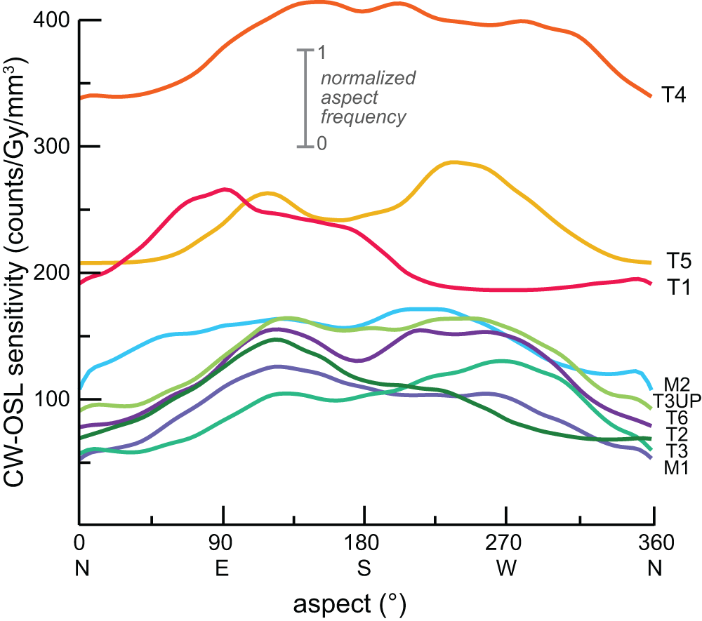
There are differences in the distribution of aspect between catchments (Fig. 8). Overall, there is a common bimodal distribution with aspects of 125° (southeast) and 225° (southwest) in most catchments. M1, T2, and T1 have a higher frequency of hillslope aspects at 125° (southeast) than at 225° (southwest). Alternatively, T3 and T5 have a higher frequency of slopes facing 225° (southwest) than 125° (southeast). T3 UP, M2, and T4 have hillslope frequencies that roughly plateau from 125° to 225° (southeast, south, and southwest). T3 UP and T4 have a greater proportion of south-facing aspects than other watersheds.
Stacked histogram displaying the aspect distribution of each sample’s catchment relative to the sample’s continuous-wave optically stimulated luminescence (CW-OSL) sensitivity (y-axis). Samples taken from the Pagliara watershed.

Figure 8 Long description
A multi-line graph. The horizontal axis label is, aspect, degree. The horizontal axis range is 0 to 360, with tick labels 0, 90, 180, 270, 360 and the letters N, E, S, W, N. The vertical axis label is, continuous wave optically stimulated luminescence sensitivity, counts slash Gy slash mm superscript 3. The vertical axis shows tick labels 100, 200, 300, 400. Text near the upper center reads, normalized aspect frequency, with a vertical scale marked 0 at the bottom and 1 at the top. Nine continuous lines are plotted and each line is identified by a text label placed near the right edge: T4, T5, T1, M2, T3UP, T6, T2, T3, M1. The lines are visually distinguished by different line colors. All lines are solid and no point markers are shown. Relative levels across the aspect range: T4 stays highest across the plot, remaining above the 300 tick and reaching above the 400 tick around the middle of the horizontal axis. T5 and T1 form the next highest group, staying around the 200 to below 300 region, with T5 rising to a broad high point near the 270 tick and T1 reaching a high point near the 90 tick before dropping toward the 180 to 270 region. M2, T3UP, T6, T2, T3 and M1 form a lower group, mostly between the 50 to below 200 region, with several of these lines rising from near the 0 to 90 region to higher values between about 90 and 270, then declining toward 360. No numeric data labels are printed on the lines and no plotted coordinates are explicitly shown.
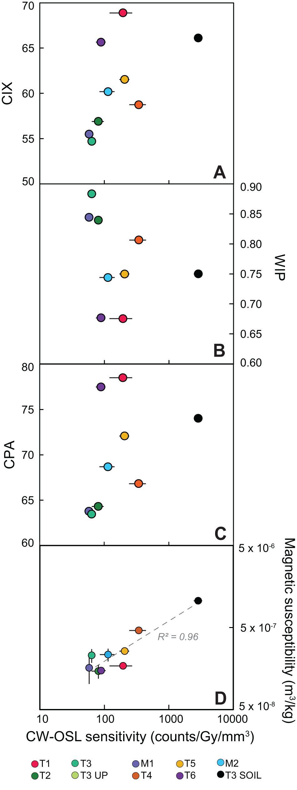
Continuous-wave optically stimulated luminescence (CW-OSL) sensitivity for samples from the Pagliara watershed versus (A) the Chemical Index of Alteration, (B) the weathering Index of Parker, and (C) the Chemical Proxy of Alteration. The CIX and CPA will increase and the WIP will decrease with chemical weathering intensity. (D) Magnetic susceptibility versus CW-OSL sensitivity.

Figure 9 Long description
A scatter plot comparing CW-OSL sensitivity (counts per Gy per mm cubed) with the Chemical Index of Alteration (CIX). The x-axis ranges from 10 to 10000 and the y-axis from 50 to 70. Data points are scattered, showing no clear trend. Panel B compares CW-OSL sensitivity with the Weathering Index of Parker (WIP), with the y-axis ranging from 0.60 to 0.90. Points are scattered similarly, indicating a weak relationship. Panel C compares CW-OSL sensitivity with the Chemical Proxy of Alteration (CPA), with the y-axis from 60 to 80. Again, the points are scattered without a strong trend. Panel D compares CW-OSL sensitivity with magnetic susceptibility (m cubed per kg), showing a strong positive correlation with an R squared value of 0.96. The x-axis ranges from 10 to 10000 and the y-axis from 5 times 10 superscript negative 8 to 5 times 10 superscript negative 6. The legend identifies samples T1, T2, T3, T3 UP, M1, T4, T5, T6, M2 and T3 SOIL, distinguished by colored markers. Panels A, B and C include horizontal error bars, while Panel D includes vertical error bars. The plots collectively show that only magnetic susceptibility has a strong relationship with CW-OSL sensitivity, while the other indices do not exhibit clear trends.
Magnetic susceptibility
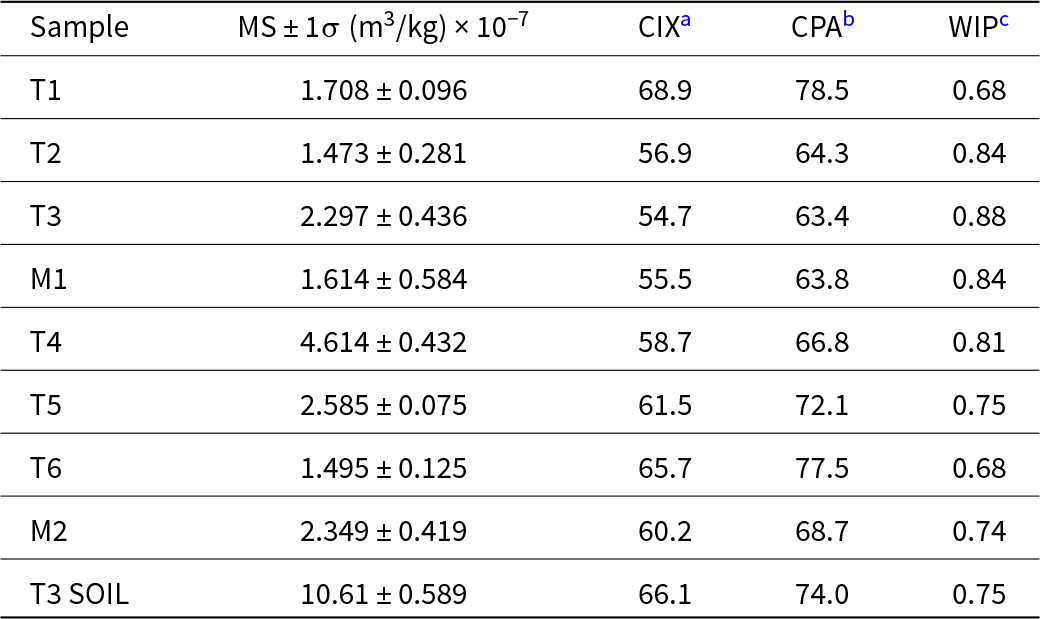
The magnetic susceptibility of the samples ranges from 1.47 × 10⁻⁷ m3/kg to 1.06 × 10− 6 m3/kg and appears to have a positive relationship to CW-OSL sensitivity (Fig. 9D, Table 4). Sample T3 SOIL has the highest magnetic susceptibility at 1.06 × 10− 6 m3/kg. The fluvial sample with the highest magnetic susceptibility is T4 at 4.61 × 10− 7 m3/kg. All other fluvial samples have magnetic susceptibility values between 1.47 × 10− 7 m3/kg and 2.58 × 10− 7 m3/kg. In addition, we note that it was observed in the field that soils displayed a high magnetic susceptibility, while bedrock displayed a low magnetic susceptibility, suggesting that magnetic susceptibility can be used as a provenance proxy for the relative recruitment of soils to the low non-weathered bedrock. Enhanced magnetic susceptibility in soil horizons, relative to the underlying parent material, is commonly attributed to atmospheric dust deposition and the in situ formation of ferromagnetic minerals through pedogenic processes (e.g., Le Borgne, Reference Le Borgne1955; Maher, Reference Maher1986).
Magnetic susceptibility (MS) results and chemical weathering indices for samples from the Pagliara watershed.

Table 4 Long description
Nine samples list magnetic susceptibility with plus or minus one sigma in cubic meters per kilogram scaled by ten to the minus seven, alongside CIXa, CPAb, and WIPc values. Magnetic susceptibility values are: T1 1.708 plus or minus 0.096, T2 1.473 plus or minus 0.281, T3 2.297 plus or minus 0.436, M1 1.614 plus or minus 0.584, T4 4.614 plus or minus 0.432, T5 2.585 plus or minus 0.075, T6 1.495 plus or minus 0.125, M2 2.349 plus or minus 0.419, and T3 soil 10.61 plus or minus 0.589. CIXa values range from 54.7 at T3 to 68.9 at T1, with T3 soil at 66.1. CPAb values range from 63.4 at T3 to 78.5 at T1, with T3 soil at 74.0. WIPc values range from 0.68 at T1 and T6 to 0.88 at T3, with T3 soil at 0.75.
a CIX, Chemical Index of Alteration.
b CPA, Chemical Proxy of Alteration.
c WIP, Weathering Index of Parker.
Proxies for chemical weathering intensity
Fluvial samples M1, T2, and T3 consistently exhibit lower weathering intensities based on CIX, CPA, and WIP values compared with the other samples in this study (Fig. 9A–C; Table 4). In contrast, T1, T3 SOIL, and T6 consistently show higher weathering intensities across all chemical weathering proxies (Fig. 9). Samples T4, T5, and M2 generally fall within the midrange of weathering intensity metrics (Fig. 9).
Discussion
Luminescence variability in nature
Our analyses reveal three orders of magnitude variability in CW-OSL sensitivity among the modern quartz samples from the Pagliara catchment. The fluvial samples have relatively dim OSL signals that decay rapidly to low background rates (Fig. 3A). The CW-OSL sensitivity has a positive relationship with the LM-OSL first-component sensitivity and the fast ratio, which is expected, as they should both be recording the initial rapid decay of the OSL signal (Fig. 4). The weaker but still positive relationship between CW-OSL sensitivity and the fast ratio is also expected due to the specific additional input of the medium component in the calculation (Durcan and Duller, Reference Durcan and Duller2011).
Many recent studies have examined variations in quartz luminescence behavior to investigate its controlling factors and potential applications for provenance and geomorphic research. Broadly, this work shows that crystallization properties initially govern the OSL sensitivity, and subsequent exposure to sedimentary processes can further enhance the OSL sensitivity (Sawakuchi et al., Reference Sawakuchi, Blair, DeWitt, Faleiros, Hyppolito and Guedes2011; Tanski et al., Reference Tanski, Rittenour, Pavano, Pazzaglia, Mills, Corbett and Bierman2024; Constantin et al., Reference Constantin, Dave, Grecu, Kabacińska, Antuzevics, Barla, Urdea, Ducea and Timar-Gabor2025). However, the degree to which sedimentary processes enhance OSL sensitivity appears to depend on the defects present in the quartz, as not all grains enhance at the same rate or magnitude (Constantin et al., Reference Constantin, Dave, Grecu, Kabacińska, Antuzevics, Barla, Urdea, Ducea and Timar-Gabor2025). Numerous studies highlight that fluvial transport (Pietsch et al., Reference Pietsch, Olley and Nanson2008; Constantin et al., Reference Constantin, Dave, Grecu, Kabacińska, Antuzevics, Barla, Urdea, Ducea and Timar-Gabor2025), coastal reworking (Sawakuchi et al., Reference Sawakuchi, Blair, DeWitt, Faleiros, Hyppolito and Guedes2011), exposure to natural fires (J. Zhang et al., Reference Zhang, Li, Sun, Tongyan, Zhou and Hao2023), and prolonged residence time in the critical zone or slow erosion rates (Sawakuchi et al., Reference Sawakuchi, Jain, Mineli, Nogueira, Bertassoli, Häggi and Sawakuchi2018; Tanski et al., Reference Tanski, Rittenour, Pavano, Pazzaglia, Mills, Corbett and Bierman2024) can enhance OSL sensitivity. With many geologic and geomorphic processes potentially contributing to quartz OSL sensitization, it remains challenging to isolate the natural controls on OSL sensitivity. In this context, our dataset from a steep, mountainous catchment, where we expect low OSL sensitivity, provides an opportunity to investigate if and potentially how quartz OSL can sensitize in an active tectonic setting. By quantifying the catchment’s geomorphic properties within its relatively simple geologic bedrock distribution, we explore potential links between landscape processes and the variability in sensitivity among samples.
Bedrock influences on OSL sensitivity
If bedrock source is the sole contributor to OSL sensitivity, we would expect samples draining different rock types to exhibit distinct OSL sensitivity values, while samples draining similar rock types would show comparable OSL sensitivity. Sample T1 exclusively sources low-grade-metamorphic rock (Fig. 2B), while T2 sources a mix of low- and high-grade metamorphic rock, yet the distribution of OSL sensitivity has a similar peak with a positive skew (Fig. 5). Adjacent catchments T5 and T6 both drain a similar mix of low- and high-grade metamorphic bedrock (Fig. 2B), yet T5 shows a broad CW-OSL sensitivity distribution, whereas T6 has two low, narrow peaks (Fig. 5), with mean values of 207 ± 36 counts/Gy/mm3 and 89 ± 15 counts/Gy/mm3 respectively. Perplexingly, M1, which should reflect the combined signals from upstream tributaries T1, T2, and T3, exhibits a unimodal distribution and lacks the positive skew or elevated OSL sensitivities observed in its tributaries (Fig. 5). These observations suggest that the OSL sensitivity inherited from bedrock may be modified in the tributaries and that the downstream signal records incomplete mixing of these contributions.
Do surface processes modulate OSL sensitivity?
There is an intriguing downstream pattern of generally decreasing OSL sensitivity, where tributaries have positively skewed distributions of OSL sensitivity (T1, T2, T3) or multiple peaks in OSL sensitivity (T4, T5, T6; Fig. 5). This is somewhat in contrast to the modern samples M1, which exhibits low OSL sensitivity and unimodal distribution, and M2, which is positively skewed but lacks significant peaks with higher OSL sensitivity (Fig. 5). This suggests that the repeated bleaching and irradiation with downstream fluvial transport does not influence OSL sensitivity. This pattern follows many recent studies that do not see a systematic increase in OSL sensitivity downstream (e.g., Capaldi et al., Reference Capaldi, Rittenour and Nelson2022; Tanski et al., Reference Tanski, Rittenour, Pavano, Pazzaglia, Mills, Corbett and Bierman2024; Constantin et al., Reference Constantin, Dave, Grecu, Kabacińska, Antuzevics, Barla, Urdea, Ducea and Timar-Gabor2025). This apparent decrease in OSL sensitivity in the mainstem relative to the tributaries could be a function of the degree of sediment mixing from tributary sources. This relationship requires some progressive downstream dilution of high-sensitivity quartz by low-sensitivity quartz in order to reduce the overall OSL sensitivity signal.
All samples show a similar prominent low peak in OSL sensitivity ∼70 counts/Gy/mm3 in their KDE curves, while few samples show significant multiple peaks at higher OSL sensitivity values (T4, T5, and T3 SOIL; Fig. 5). Additionally, all three of these samples (T4, T5, and T3 SOIL) show high values of magnetic susceptibility and generally trend to more intense chemical weathering relative to the other samples (Figs. 5 and 9). We expect higher magnetic susceptibility and chemical weathering in the soil samples relative to the fluvial samples. The fact that OSL sensitivity follows this pattern may suggest that the OSL signalmay also be sensitive to soil formation processes or residence time along hillslopes (e.g., Tanski et al., Reference Tanski, Rittenour, Pavano, Pazzaglia, Mills, Corbett and Bierman2024). Although we only have one hillslope soil sample, the contrast in OSL sensitivity between the soil and the fluvial sediment may be indicative of how hillslope processes such as soil development, prolonged exposure to charge-trapping radiation, or bioturbation contribute more to OSL sensitivity changes than fluvial processes.
Differences in transport and storage along hillslopes and channels may dilute the highly sensitized grains found in hillslope soils and a few tributaries. Catchments with lower normalized channel steepness (k sn) show more variable and multi-peaked KDEs of OSL sensitivity (T1, T4, T5, T6, M2), suggesting that steepness-driven differences in sediment sourcing and routing shape OSL sensitivity patterns. The hypsometric integral (HI) also shows a negative relationship with CW-OSL sensitivity, especially if T4 is excluded (Fig. 6F). High-HI catchments, which are steep, high-relief basins dominated by higher elevations, are more susceptible to landsliding and rapid transport, whereas low-HI catchments likely allow longer sediment storage and slower transport, promoting longer duration of charge trapping and bleaching. Hillslope aspect may further influence weathering through insolation-driven microclimates (e.g., Yimer et al., Reference Yimer, Ledin and Abdelkadir2006; Inbar et al., Reference Inbar, Nyman, Rengers, Lane and Sheridan2018). Most catchments show unimodal or bimodal aspect distributions, but T4 and T3 UP are strongly south-facing (Fig. 8). T4 exhibits the highest OSL sensitivity and magnetic susceptibility of the fluvial samples (Fig. 9D), which may suggest that south-facing microclimates with distinct wet−dry cycles or weathering regimes (e.g., Rech et al., Reference Rech, Reeves and Hendricks2001; Burnett et al., Reference Burnett, Meyer and McFadden2008) may enhance quartz OSL sensitization. Overall, these geomorphic factors appear to influence OSL sensitivity, but their relative contribution and the role of alternative controls remain uncertain.
If OSL sensitization is occurring in hillslope soils, these sensitized grains appear to be diluted before entering the fluvial network. Both landslide activity and fluvial bedrock erosion may contribute to this dilution. All catchments in the Pagliara watershed display slightly negatively skewed normalized slope distributions (Fig. 7), indicative of landslide-to-wash-dominated hillslopes (e.g., Wolinsky and Pratson, Reference Wolinsky and Pratson2005). Aerial imagery reveals the presence of recent bedrock landslides across the catchment, which would introduce minimally weathered bedrock into the system and could dilute any enhanced OSL sensitivity grains derived from the hillslope soils. In addition, the Pagliara catchment has high rates of erosion at 1–2 mm/yr (Cyr et al., Reference Cyr, Granger, Olivetti and Molin2010; Pavano et al., Reference Pavano, Pazzaglia, Rittenour, Catalano, Corbett and Bierman2024), and rapid incision along the fluvial network can also introduce minimally weathered bedrock.
Conclusion
We investigate the OSL sensitivity of quartz sand within a small, tectonically active catchment in Sicily using modern fluvial samples and a hillslope soil sample. We assess the relationships between OSL sensitivity and magnetic susceptibility, chemical weathering indices, bedrock lithology, and topographic metrics. OSL sensitivity varies by three orders of magnitude across the watershed, which is interpreted to reflect contrasts in bedrock versus soil contributions, geomorphic setting, and progressive dilution and mixing as sediment is transported downstream.
Bedrock lithology likely establishes the initial quartz OSL sensitivity through crystalline defects and impurities formed during crystallization. However, substantial variability among samples indicates that lithology alone cannot account for the observed patterns. Importantly, our results highlight that a hillslope soil sample has an order-of-magnitude-greater quartz OSL sensitivity than all fluvial sediment, suggesting that OSL sensitivity enhancement is primarily driven by hillslope or pedogenic processes. Positive relationships between OSL sensitivity, magnetic susceptibility, and chemical weathering indices further support the idea that prolonged residence in soils can promote quartz OSL sensitization.
In contrast, fluvial samples exhibit low OSL sensitivity, sometimes positively skewed toward higher OSL sensitivity values, and show a pattern of decreasing OSL sensitivity with downstream distance. We interpret this downstream decline as evidence that high OSL sensitivity quartz grains derived from hillslope soils are progressively diluted by low OSL sensitivity quartz supplied by deep-seated landslides and bedrock incision in this steep, rapidly eroding catchment. Catchments with high channel steepness and high hypsometry, conditions that promote landslides and rapid erosion, tend to produce sediment with lower OSL sensitivity than the catchments with lower channel steepness and hypsometry. As sources of low OSL sensitivity grains mix into the mainstem they dominate the downstream signal and obscure contributions from sources that contribute high OSL sensitivity grains.
Together, these results suggest a hierarchy of controls: bedrock lithology provides the initial quartz OSL sensitivity, hillslope pedogenic processes enhance the OSL sensitivity of the bedrock, and hillslope and fluvial transport processes modulate that material through dilution, storage, and mixing. This hierarchy may explain why tectonically active catchments often lack OSL-sensitized quartz grains, as rapid erosion, limited storage, and frequent sediment evacuations suppress the potential processes that enhance OSL sensitivity while simultaneously diluting any sensitized material that is produced. Future studies that broaden sampling across varied climatic and tectonic settings and incorporate more soil data and residence time constraints will be crucial for resolving how sediment dilution, storage, and routing collectively shape OSL sensitivity.
Acknowledgments
The authors thank Harrison Gray, Amanda Keen-Zebert, and one anonymous reviewer for their constructive feedback on the article.
Financial support
Funding was provided by Utah State University’s Undergraduate Research and Creative Opportunities Grant to JRM, NSF-EAR-1904278 to TMR, and NSF-EAR-1904262 to FJP.
Competing interests
The authors declare that they have no conflict of interest.