1. Introduction

Brine rejection during sea-ice formation plays a critical role in the increase of wintertime salinity over the continental shelf that is necessary for the formation of bottom water. Polynyas are regions where the rate of sea-ice formation may be up to 10 times greater than in the surrounding sea-ice zone (Reference Zwally, Comiso, Gordon and JacobsZwally and others, 1985). A detailed census of the significant polynyas between 40° and 160° E, using satellite passive-microwave data over an 8 year period, shows that the largest and most persistent polynyas are the Shackleton Ice Shelf and the Mertz polynyas, with an average area in winter of 30 000 and 23 000 km², respectively (Reference Massom, Harris, Michael and PotterMassom and others, 1998). However, in spite of its larger size the Shackleton Ice Shelf (near 95° E) is not associated with bottom water formation (Reference Bindoff, Rosenberg and WarnerBindoff and others, 2000a). The factors that affect ice production, and therefore brine rejection, are not limited to the size of the polynya alone, but also include the strength and direction of the local winds, and air and water temperatures. Along the Antarctic coastline, the Mertz polynya (67° S, 145° E) is in a region of some of the world’s strongest and most persistent winds (Reference BallBall, 1957; Reference Adolphs and WendlerAdolphs and Wendler, 1995). It is these intense meteorological conditions that give rise to the Mertz polynya having what is believed to be the greatest ice production in East Antarctica (Reference Cavalieri, Martin and JacobsCavalieri and Martin, 1985).

The Mertz polynya lies immediately above the Adelie Depression (Fig. 1) and forms to the west of Mertz Glacier. Its size is also partly controlled by the line of grounded icebergs and fast ice that extends north from this glacier (at 146° E), blocking the westward flow of sea ice into the polynya area. The katabatic winds are strongly offshore at the coastline, turning westwards within 20−30 km. However, the ice-free region extends well beyond the zone of strong winds, and this polynya (-200 km wide) is wider than most (Reference Massom, Harris, Michael and PotterMassom and others, 1998). Its unusual width is partly caused by the shape and northward orientation of Mertz Glacier Tongue blocking the westward transport of sea ice. However, the polynya also becomes ice-free earlier in the spring than locations immediately to the east and west (Reference Gloersen, Campbell, Cavalieri, Comiso, Parkinson and ZwallyGloersen and others, 1992; Reference Massom, Harris, Michael and PotterMassom and others, 1998), which may be the result of the upwelling of warm modified circumpolar deep water (MCDW) in the polynya region (Reference Rintoul, Jacobs and WeissRintoul, 1998). The polynya has a strong seasonal signal, with its areal extent typically becoming largest in October, ranging from 20 000 to 60 000 km² (Reference Massom, Harris, Michael and PotterMassom and others, 1998). Its fastest rate of growth tends to occur during August-September, which is consistent with observations of maximum sea-ice production and coincides with the colder bottom waters observed in temperature time series measured offshore (Reference FukumachiFukamachi and others, 2000).

Fig. 1.

The Terre Adélie coastline from 142° to 147° E, showing the geographical setting for the Mert zPolynya experiment and in particular the Adelie Depression and Mertz Glacier. The locations of the CTD stations along the western edge of Mertz Glacier are shown for repeat 3 of this section (stations 79−89). (Inset: the location of Mertz polynya in Antarctica.)

The Australian-Antarctic basin is associated with bottom water formation off the Terre Adelie coastline near 140° E (Reference Gordon, Tchernia and HayesGordon and Tchernia, 1972). However, this source has been considered relatively weak, and the bottom waters found in this basin were thought to be the product of mixing between Ross Sea bottom water (RSBW) and Weddell Sea bottom water (WSBW) (Reference Carmack and AngelCarmack, 1977). However, recent hydrographic observations along 140° E have shown a local maximum in bottom CFC-11 and oxygen concentrations, and a minimum in bottom temperatures (Reference Bindoff, Warner and NicolBindoff and others, 1997; Reference Rintoul and BullisterRintoul and Bullister, 1999). This maximum in CFC-11 and oxygen concentrations cannot be obtained by mixing RSBW and WSBW in this basin, because both of these water masses have lower CFC-11 and oxygen concentrations and warmer temperatures in this basin. This suggests that the bottom waters in this basin have a local source. The identification of a source of bottom water on the continental shelf in the Adélie Depression near Mertz Glacier (Reference Gordon, Tchernia and HayesGordon and Tchernia, 1972; Reference Rintoul, Jacobs and WeissRintoul, 1998) led to a reinterpretation of the volumetric census of bottom waters. This showed that Terre Adelie bottom water has a volume second only to WSBW and three times that of RSBW (Reference Rintoul, Jacobs and WeissRintoul, 1998).

This paper presents the first wintertime hydrographic sections taken in this important source region of Antarctic bottom water. We describe the distribution and circulation of water masses present along three repeats of a hydrographic section across the Adelie Depression. We then develop a simple model of the major processes of interactions with the atmosphere and ice shelf operating within the Mertz polynya that are responsible for forming the observed wintertime water masses.

2. Description of the Study Area

3. Property Distributions and Circulation

The temperature and salinity section along Mertz Glacier from the third and first repeats of the section (Figs 2 and 3, respectively) shows four distinct water masses and two frontal systems. This section was collected towards the end of the voyage (19−21 August) after an intense outbreak of cold air temperatures off the continent. The warmest waters (>−1.88°C) are observed on the northern side of the Adelie Depression, and the coldest at the southern end (<−2.0°C). The coldest waters form a local minimum at 300 dbar adjacent to the continent.

Fig. 2.

The potential temp>erature field (°c) along the section taken on repeat 3 CTD station numbers are shown along the top, the x axis representing the distance along mertz glacier from the northwest tip (top right corner) to the antarctic coast. isotherms are contoured from average 2 dbar CTD data, and the bottom topography from maximum pressures recorded by the CTD. isotherms are the thin lines, and the thick lines are the iso_pycnals separating the water masses shown in table 1.

Fig. 3.

The salinity field (_psu) along the section taken on repeat 1 (stations 22−31). the station locations are the same as those for repeat 3 shown in figure 1.

While the temperature section along Mertz Glacier is relatively simple, the salinity section is more complex. This is best seen in repeat 1 (Fig. 3), where the freshest waters occur near the surface to the north and progressively increase in salinity through a front into a region of very uniform salinity that extends from near the surface to 300−400 dbar. Further south, there is another strong gradient in salinity, with the fresher values observed close to the continent. The most saline waters in this experiment (>34.7psu), were found below a relatively homogeneous layer located over the middle of the depression and its northern flank.

In the salinity section, two fronts were observed. The first occurs on the northern side of the depression between stations 26 and 27. On the southern side of the depression there is a second front between stations 29 and 30. All three repeats of this section showed these two fronts. Although their position varied on each occupation, they are typified by a single potential density contour (Table 1). Both the northern and southern fronts are associated with a 27.88 kg m-³ potential density surface (Figs 2 and 3, shown as thick contours). The thick, relatively homogeneous water that lies between these two fronts is bounded at depth by the 27.91 kg m-³ potential density surface.

Table 1.

the major water masses that were found along the edge of mertz glacier in winter and their definitions in terms of potential density. also shown are area-averaged potential temperature and salinity for the three repeat sections

These horizontal gradients in the salinity (and hence density field) imply significant vertical shear in the ocean currents through this section. However, because of the difficulty in determining the precise reference velocity to use with the density field alone, we have used the horizontal components of the surface velocities from the ADCP measurements rotated normal to the section. The ADCP coverage along the section is not always complete, so the ADCP reference velocity field has been averaged over all three repeats of this section. This averaged reference velocity has been added to the geostrophic velocity field obtained by integrating the thermal wind equations from the surface to the ocean floor. In this way, the horizontal velocity through each vertical section was formed (third repeat is shown in Fig. 4). The maximum rms variability of the averaged ADCP velocities of about 9 cm s⁻¹ is an estimate of the uncertainty in the surface reference velocity (and velocity field at depth).

Fig. 4.

The geostrophic velocity field (cm s₋₁) normal to the section along mertz glacier for repeat 3, referenced to the average surface adcp velocities.

The ADCP surface reference (at 20 dbar) is quite large compared to the contribution to the velocity from the thermal wind equations and makes the velocity field largely barotropic. In the following, the flow is examined in terms of the velocity component normal to the section. Although the section does not run north-south, the direction of this component will subsequently be expressed as either eastward or westward. On the northern side of the Adelie Depression in ocean depths shallower than 500 dbar the flow field is westward (out of page). Over the Adelie Depression in ocean depths of > 500 dbar the direction of the flow field changes to eastward, i.e. into Mertz Glacier, before returning westward again in the shallower waters near the Antarctic continent. This westward return flow adjacent to Antarctica is where the flow is strongest, exceeding 20 cm s−1 and is quite narrow compared to the currents to the north.

4. Water Masses

We identify four distinct water masses in the CTD data in this section. The relatively warm, fresh and oxygen-poor water found north of the northern front is termed highly modified circumpolar deep water (HMCDW) (Figs 5 and 6). The relatively homogeneous and non-stratified water between the two fronts is called winter water (WW), and the cold water south of the southern front is called ice-shelf water (ISW). The densest water that lies in the Adélie Depression is typically deeper than 500 dbar and bounded above by a 29.1 kg m−3 potential density surface, and is termed high-salinity shelf water (HSSW). The bounding properties for each of these four water masses are listed in Table 1 and are marked in Figures 2–4.

Fig. 5.

6−s Scatter plot of all 2 dbar ctd data collected along the section (stations 22−3146−56, 79−92). lines of constant σ_θ are superimposed (dashed line) to highlight water-mass boundaries defined in table 1. shown also is the surface freezing-point curve (continuous line).

Fig. 6.

02−s scatter plots of all ctd bottle data collected on all three sections (stations 22−31, 46−56, 79−92).

These definitions differ from those of Reference Rintoul, Jacobs and WeissRintoul (1998) and Reference Whitworth, Orsi, Kim, Nowlin, Jacobs and WeissWhitworth and others (1998), but are consistent with the frontal locations and boundaries of the water masses observed in winter. HMCDW is equivalent to the densest varieties of MCDW presented in the nomenclature of Reference Whitworth, Orsi, Kim, Nowlin, Jacobs and WeissWhitworth and others (1998). Our WW and HSSW are both dense enough to be classified as shelf water in their scheme. The key distinction between our WW and HSSW is that WW is weakly stratified while HSSW is more strongly stratified and much saltier (> 34.66 psu).

The potential temperature and salinity diagram shows a strong relationship between HMCDW, WW and HSSW (Fig. 5). HMCDW, WW and HSSW have a broadly linear relation between the coldest and saltiest forms of HSSW and the warmest and freshest forms of HMCDW. The HSSW shows the least scatter from this linear relation, consistent with the water mass being isolated from the atmosphere (at the time of collection). Although the HSSW is colder than the surface freezing point, it is not supercooled compared with the freezing temperature at 40 dbar, suggesting that it was formed near the surface (unlike ISW). The WW (27.91−27.88 kg m⁻³ potential density) shows much more scatter from this linear relationship, being both warmer and cooler. The warm varieties of the WW occurred in repeat 2 when temperatures in the region were relatively high, and the cold forms of WW are actually slightly supercooled, reflecting contact with Mertz Glacier. It is likely that this variability in the WW properties and its low stratification reflects the interaction of this water mass with the atmosphere or ice shelf. The fourth water mass, ISW, is very distinctive as a result of being much colder ( <−2.0°C) than the other three water masses. This water is sufficiently cold to have originated from beneath Mertz Glacier. ISW does not belong to the linear relation between HSSW and HMCDW, and its properties are a result of its contact with Mertz Glacier.

A similar linear relation can be clearly seen in the oxygen concentration and salinity diagram (Fig. 6). HMCDW has the lowest concentrations of oxygen. Through the ocean-atmosphere interaction of the polynya processes, the oxygen concentration increases linearly through the conversion of the HMCDW (-82% saturation) into WW and HSSW (∼ 8 8% saturation). Although the HSSW is cut off from the atmosphere, it is higher in both salinity and oxygen, suggesting that it could have formed earlier in the winter prior to these measurements. As found in t-s space, the oxygen concentration of the ISW places it off the linear relation between HMCDW and HSSW. Note also that the oxygen concentration of ISW is slightly less than that in W W and significantly less than that in HSSW. Interestingly all four water masses are well beneath the oxygen saturation limit of approximately 380 μmol kg⁻¹ prescribed by the temperature range of the samples.

5. Discussion

The area-averaged properties of cross-sectional area, salinity, temperature, oxygen concentration, velocity and mass transport (normal to the section along Mertz Glacier) are presented for the individual water masses, in each section, in Table 2. The distribution of these water masses and their variability and transport through the sections suggests an overall pattern of circulation. The HMCDW is moving westwards along the shelf break north of the polynya with a transport of 0.7 Sv. The linear relation on the temperature−salinity diagram suggests that the WW waters are derived from the HMCDW. This transformation occurs through the direct interaction of the HMCDW with the cold atmosphere in the polynya region. The loss of heat and brine rejection from the formation of sea ice causes vertical convection within the WW layer, leading to a relatively salty and vertically homogeneous water mass. WW has the greatest cross-sectional area, of ∼ 2 × 10⁷ m², and is about twice the area of HMCDW, four times the area of ISW and twice the area of HSSW. Both WW and HSSW flow eastwards through the section, with a transport of 1.1 and 0.9 Sv, respectively, for a total of 2 Sv. These waters are modified by their interaction with Mertz Glacier and cooled and freshened to form ISW. About 6 0% of these two eastward-flowing water masses return as the fast narrow ISW current of 1.2 Sv against the Antarctic continent (Fig. 4).

Table 2.

Cross-sectional area averaged properties for the water masses designated in Table 1 along the section shown in Figure 1

Using this circulation pattern, a simple model (Fig. 7) was developed for estimating the ice production and heat flux of the entire polynya/glacier system for which we chose two distinct flow patterns. The first is associated with the observations taken during the experiment, where HMCDW is converted initially into WW and then into ISW (Fig. 7b). The pycnocline separating WW from the underlying HSSW (Fig. 3) suggests that these water masses were not actively mixing together during the experiment, and the reduction in cross-sectional area of WW by 5 0% during the experiment supports this idea (Table 2). The second flow pattern is associated with a time period prior to the voyage (Fig. 7a) where there is active formation of HSSWand it interacts with Mertz Glacier to form ISW. This flow pattern represents the process that would create the greatest brine rejection from sea-ice formation.

Fig. 7.

Model of the exchange between HMCDW, WW, HSSW and ISW used to estimate heat and fresh-water transports. (a) Scenario prior to the voyage where WW exchanges with HSSW which then exchanges with ISW (b) Scenario during voyage where WW exchanges directly with ISW

Although the volume transports through the section for each of the water masses shown in Table 2 vary significantly (0.2−1.5 Sv), we have assumed that the volume exchange (Q_mass) between all water masses and for both flow patterns is constant. The flux of heat (Qheat) and freshwater (Qfreshwater) through the surface area of the polynya (Ap) between two water masses can then be calculated as,

where θ and S are the observed area-averaged potential temperature and salinity values for each water mass. The subscripts indicate the different water masses. The S₀ term in Equation (2) is the average salinity between the two water masses for which the fresh-water exchange is being calculated. These equations are a simplification of the equations used to calculate heat and fresh-water transports beneath the Amery Ice Shelf by Reference Wong, Bindoff, Forbes, Jacobs and WeissWong and others (1998). The greatest mass transport, found for WW, is 1.458 Sv eastwards, with the other water masses approximately half this value. The total transport across the section was calculated and indicates that for each repeat there is a mass imbalance into the section of 0.01−0.81 Sv.

The size of the Mertz polynya has been estimated using passive-microwave data as ∼ 2 0 000 km² (Reference Massom, Harris, Michael and PotterMassom and others, 1998). This area, approximately defined by the 100 km length of the glacier and a width 200 km to the west, is much larger than the actual open-water area available to interact directly with the atmosphere during the experiment (Reference Massom, Hill, Lytle, Worby, Paget and AllisonMassom and others, 2001, fig. 1 and table 1). Here we choose the effective open-water area, A_p, to be 20% of the reported area, or 4000 km², to represent the total open-water component fraction of the polynya. This open area represents an average ice concentration of 80% and can be quite variable in space and season. The results presented in Table 3 are sensitive to this estimate of open area. A mass exchange (Q_mass) of 1.45 Sv between water masses was chosen. These two choices are somewhat arbitrary, but are consistent with the mass transport of WW and the mass exchange required to give the observed sea-ice growth in the polynya region (Reference LytleLytle and others, 2001).

Table 3.

fresh-water and heat exchanges using equations (1) and (2) for the area-averaged water-mass properties sampled from repeat 1( table 2)

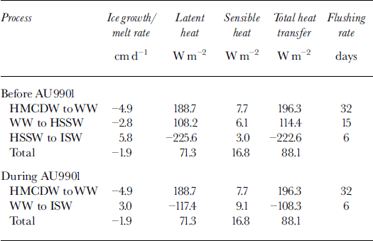
Using these parameters, and Equations (1) and (2), the "during-voyage" ice-production rate and heat flux out of the polynya are estimated to be 4.9 cm d⁻¹ and 196.3 W m⁻², respectively. In the scenario suggested for the period prior to the voyage, when the polynya processes were strong enough to produce HSSW, the corresponding results were 7.7 cm d⁻¹ and 310.7 Wm"² Sea-ice production rates estimated from direct observations of the sea-ice conditions during the voyage are approximately 7 cm d⁻¹, and in more extreme conditions could reach 10 cm d⁻¹ (Reference LytleLytle and others, 2001). Because of the high salinity of the sea ice (∼10psu), 7 cm d-¹ represents ∼5 cm d⁻¹ of fresh water.

The total heat exchange includes the sensible-heat contribution from advection between the water masses and the latent heat associated with the formation of sea ice. The sensible-heat contribution in converting HMGDW to WW is about 7.7 W m⁻² and represents only 3.9% of the total heat budget required for this conversion of 196.3 W m⁻² (Table 3). Similarly, for the conversion of WW to HSSW in the "before-voyage" scenario, the sensible heat is just 6.1 W m⁻² and represents 5.3% of the total heat budget. This low contribution occurs because the HMGDW is almost at freezing temperature and thus there is little scope for heat exchange between HMGDW and WW (or HSSW) through advection. By comparison, the salinity differences between HMGDWand WWor HSSWare large, and in terms of brine rejection imply large heat losses to the atmosphere from the ocean through sea-ice formation.

Although the ocean heat fluxes are small (13.8 W m⁻² for HMCDW to HSSW and 7.7 W m⁻² for HMCDW to WW) compared to the latent-heat fluxes, they are in good qualitative agreement with other direct and indirect measures of ocean heat fluxes. Reference Lytle, Massom, Bindoff, Worby and AllisonLytle and others (2000) estimate ocean heat fluxes of 13.0−14.5 W m⁻² over the Antarctic Divergence at 140° E. In the Weddell Gyre, Reference Fahrbach, Rohardt, Schroder and StrassFahrbach and others (1994) estimate 19 W m⁻² , while from observations of fast ice, Reference Heil, Allison and LytleHeil and others (1996) found a heat-flux range of 0−18 W m⁻². Similarly, the estimates of ocean heat fluxes inferred from models are 5−30 Wm"² depending on the season (Reference Wu, Simmonds and BuddWu and others, 1997).

The production of ISW is normalized to the area of the polynya for comparison with the sea-ice production rate. We find that in terms of the complete Mertz polynya/glacier system, the contribution of fresh water and heat loss from the base of the glacier are respectively 3.0 cm d⁻¹ and 108.3 W m⁻² during the voyage and 5.8 cm d⁻¹ and 222.6 W m⁻² at the time of HSSW formation.

The net fresh-water input from the Mertz polynya/ glacier system is the sum of the contributions from the ice production in the polynya and meltwater from the glacier. In the case of the before-voyage and during-voyage flow patterns, the meltwater from Mertz Glacier compensates 75% and 61% of the brine production from sea-ice formation, respectively. In both scenarios the sea-ice production is greater than the input of glacier meltwater, but close enough to suggest that during summer the region may be a net exporter of fresh water.

However, we found that of the four water masses reported here, ISW experienced the greatest change in cross-sectional area-averaged salinity and temperature over the period of the experiment, becoming steadily fresher (34.61−34.59) and significantly colder (-1.91° to −1.94°C). This result could be explained by the recirculation of waters beneath the glacier, increasing the loss of heat and injection of fresh water, but implies that the greatest uncertainty in our estimates of the net fresh-water flux is the meltwater contribution from Mertz Glacier. Our estimate of this contribution (for the conversion of WW to ISW), 44 Gt a⁻¹, is more than twice the melt rate estimated for Amery Ice Shelf, 10−21.9 Gt a"¹ (Reference Wong, Bindoff, Forbes, Jacobs and WeissWong and others, 1998).

The estimated flushing times of each of the water masses give an indication of how quickly each water mass could be overturned. WW has the largest cross-sectional area (and therefore volume), and subsequently has the longest flushing time of 32 days, while ISW has the shortest flushing time of 6 days. These time-scales are short enough for the seasonal cycle to control the wintertime water-mass distributions over the shelf and are consistent with the absence of WW during summer.

6. Conclusions

The calculations of ice production (4.9−7.7 cm d−¹ fresh­water equivalent) and corresponding heat transfer (196−310 W m⁻²) from the Mertz polynya, using fresh-water and heat-transport analysis of the water-mass properties sampled along the western edge of Mertz Glacier, are consistent with sea-ice observations. The WW and HSSW constitute most of the water found in the depression and are found to have an easterly flow. This flow is in almost the opposite direction to the drifting buoys deployed in the same area (Reference LytleLytle and others, 2001) and suggests that locally the circulation of WW is controlled by pressure gradients within the water column rather than by the local winds.

A number of questions arise from this study regarding the mechanism of bottom water formation from the Mertz polynya area. The salinity of the WW is sufficiently high to become bottom water (Reference Bindoff, Rintoul and MassomBindoff and others, 2000b). Unlike HSSW, this water is not trapped by the Adélie Depression, but it is possible that the volume of HSSW does increase sufficiently to spill out of the trough and down the continental slope. The question of how and when HSSW is formed is also important. Although the RSV aurora australis was in the polynya for 1 month during winter, none of the CTDs revealed convection through the entire water column in the depression. This suggests that HSSW was formed either earlier in the season, or over shallow topography ( <100 dbar) and then drained into the depression.