


1. Introduction
Population aging is increasing demand for aged care services in Australia. Older people are more likely to experience disability, chronic conditions, cognitive impairment, and complex care needs, which increases the likelihood of requiring formal support in later life (Australian Bureau of Statistics, 2024; Australian Institute of Health and Welfare, 2024a). Residential aged care (RAC) is therefore a central part of the care system for older Australians whose needs can no longer be met adequately in the community. In this setting, stronger evidence on duration in care is important for planning, funding, and resource allocation (Australian Government Department of Health and Aged Care, 2026; Fracalossi et al., Reference Fracalossi, Zhang, Lee and Shi2025; Zhang et al., Reference Zhang, Shi and Huang2023). Length of stay (LOS) is especially important because it affects bed demand, staffing requirements, case-mix management, long-term expenditure, and the valuation of aged-care liabilities. At the resident level, LOS reflects the joint role of physical dependency, behavioral symptoms, psychological wellbeing, and medical complexity after admission.
Beyond its operational relevance, LOS is also an actuarially important component of long-term care risk. In retirement and aged-care systems, duration in care shapes the timing and magnitude of future cash flows and therefore affects the projection of long-dated care liabilities, expenditure commitments, and funding requirements. From this perspective, modeling LOS is not only a question of service utilization, but also one of measuring how heterogeneity in long-term care trajectories translates into retirement-related financial risk. More broadly, actuarial work at the finance–insurance interface has emphasized that long-dated liabilities are jointly shaped by biometric and financial risk, including longevity risk and market-consistent valuation considerations (Bacinello et al., Reference Bacinello, Millossovich and Chen2017, Reference Bacinello, Chen, Sehner and Millossovich2021).
This paper studies LOS in Australian RAC using historical data from the Australian Aged Care Funding Instrument (ACFI). Our central research question is whether detailed assessment and diagnosis information improves the prediction of LOS beyond demographic characteristics and broad measures of care need. In addressing this question, the paper targets two related gaps in the literature. The first is empirical. The second is methodological. This actuarial perspective is especially relevant in the context of retirement risk, where long-term care needs represent an important channel through which biometric risk generates persistent financial obligations. Better modeling of LOS can therefore improve not only statistical prediction but also the measurement of heterogeneity in long-term care duration risk for forecasting, liability assessment, and resource planning. This is especially important where long-term care needs form part of the broader financial challenge of retirement provision, since uncertainty in care duration directly affects the scale and timing of future obligations.
The empirical gap concerns the role of detailed clinical information in predicting LOS. Existing RAC studies have established the importance of age, sex, admission timing, dementia, and the broad ACFI domains (Fracalossi et al., Reference Fracalossi, Zhang, Lee and Shi2025; Xu & Yan, Reference Xu and Yan2025; Zhang et al., Reference Zhang, Shi and Huang2023). However, they provide limited evidence on the additional predictive role of more detailed mood-related and diagnosis variables. This gap matters because the ACFI contains information that goes well beyond broad care-need categories. In addition to the core domains of Activities of Daily Living (ADL), Behavior (BEH), and Complex Health Care (CHC), ACFI records chronic mood disturbance, the Cornell Scale for Depression (CSD) score, and detailed mental-behavioral and medical diagnoses (Australian Government Department of Health, 2020). These variables may matter for LOS because they capture dimensions of resident need that are not fully reflected in demographics, dementia status, or domain-level dependency alone. From an actuarial perspective, this richer information may also improve the representation of heterogeneity in long-term care duration risk, which is central to forecasting care costs and related liabilities.
The case for these richer variables is substantive as well as statistical. Depression and related symptoms are common in RAC and may affect functioning, social engagement, care needs, and overall quality of life (Australian Institute of Health and Welfare, 2024b; Sakai et al., Reference Sakai, Jadczak, Visvanathan, Schultz and Inacio2024). This psychosocial dimension is especially relevant during the transition into residential care, which often involves loss of independence, bereavement, loneliness, and reduced social connection (Scott et al., Reference Scott, Raynor, Dare, Grieve and Costello2024; Tan et al., Reference Tan, Maneze, Montayre, Ramjan, Wang and Salamonson2023). Mood disturbance should therefore not be viewed only as a quality-of-life outcome. It may also shape subsequent care trajectories and duration in care through its interaction with behavior, frailty, dementia, and broader clinical complexity. The Cornell Scale is also of direct relevance here, because recent evidence continues to support its usefulness in identifying depression among older people with dementia (Atchison et al., Reference Atchison, Nazir, Wu, Seitz, Watt and Goodarzi2024). Historical ACFI data are therefore especially valuable for studying heterogeneity in LOS, even though the funding system has since shifted from ACFI to AN-ACC (Australian Government Department of Health and Aged Care, 2026; Fracalossi et al., Reference Fracalossi, Zhang, Lee and Shi2025). More broadly, recent work on institutional long-term care suggests that duration of stay and care intensity are closely linked, which further strengthens the case for a richer representation of resident need (Bladt et al., Reference Bladt, Fuino, Shemendyuk and Wagner2023). This broader actuarial context also includes work on long-term care and retirement-related products, including valuation of long-term care options embedded in life annuities (Chen et al., Reference Chen, Fuino, Sehner and Wagner2022), longevity-linked post-retirement benefit design (Olivieri & Pitacco, Reference Olivieri and Pitacco2020), and modeling the burden of institutional long-term care using duration and intensity (Bladt et al., Reference Bladt, Fuino, Shemendyuk and Wagner2023). Our paper complements this literature by focusing on resident-level heterogeneity in care duration as an actuarially important driver of long-term care risk.
The methodological gap lies in how LOS is modeled. Length of stay is typically observed as a censored time-to-event outcome rather than as a conventional complete variable. However, the existing literature does not fully combine rich resident-level ACFI information with a flexible survival framework. Specifically, in the Australian RAC literature, Zhang et al. (Reference Zhang, Shi and Huang2023) analyze LOS using a weighted Cox model that is limited to linear effects, whereas Fracalossi et al. (Reference Fracalossi, Zhang, Lee and Shi2025) apply more flexible machine-learning methods but to observed LOS in complete-case data only. Thus, they do not comprehensively address three main features of LOS modeling: right-censoring, potentially complex nonlinear relationships, and strong interdependence among ACFI-based predictors. This modeling issue is also relevant in light of the broader healthcare literature, which has highlighted the value of flexible machine-learning methods when clinical data are high-dimensional, nonlinear, and heterogeneous (Kolasa et al., Reference Kolasa, Admassu, Hołownia-Voloskova, Kędzior, Poirrier and Perni2024). More generally, from an actuarial perspective, restrictive modeling assumptions may also create model risk when long-term care duration is used to support liability assessment, expenditure forecasting, and resource planning.
Our empirical analysis uses comprehensive ACFI administrative records spanning 2008–2022. After standard sample preprocessing, the final sample contains more than 1.5 million observations. To model LOS, we include a rich set of covariates covering sex, admission year, age group at admission, the three core ACFI domain scores and their categorical levels, the CSD, chronic mood disturbance, and grouped mental-behavioral and medical diagnosis measures. This information set is considerably richer than that used in the existing literature and therefore provides a stronger basis for analyzing LOS in residential aged care and for understanding heterogeneity in long-term care duration risk.
The paper proceeds in two analytical stages. We first document the main features of the data that are relevant for model selection. Our preliminary analysis indicates pervasive violations of the proportional hazards assumption, clear nonlinearity in continuous covariates, and strong dependence among predictors. These features motivate a flexible survival-learning approach beyond those used in the existing literature (Fracalossi et al., Reference Fracalossi, Zhang, Lee and Shi2025; Xu & Yan, Reference Xu and Yan2025; Zhang et al., Reference Zhang, Shi and Huang2023). We therefore model LOS using the accelerated oblique random survival forest (AORSF) proposed by Jaeger et al. (Reference Jaeger, Welden, Lenoir, Speiser, Segar, Pandey and Pajewski2024). Unlike standard Cox-type models, this framework is designed for right-censored outcomes and can flexibly accommodate nonlinear effects and complex interactions. Relative to axis-aligned survival forests, oblique splits are particularly well suited to our setting because the ACFI variables are strongly related by construction and capture overlapping dimensions of care need, mood disturbance, and diagnosis burden (Berkowitz et al., Reference Berkowitz, Altman and Loughin2024; Jaeger et al., Reference Jaeger, Long, Long, Sims, Szychowski, Min, Mcclure, Howard and Simon2019; Menze et al., Reference Menze, Kelm, Splitthoff, Koethe and Hamprecht2011). We then examine variable importance, interaction patterns, and heterogeneity across care-need profiles, admission cohorts, and age groups.
The paper makes three contributions to the actuarial analysis of residential aged care and long-term care risk. First, it helps fill the empirical gap by extending the RAC literature to incorporate detailed mood-related and diagnosis information from the ACFI. Second, it addresses the methodological gap by applying a flexible survival machine-learning framework to the Australian RAC LOS setting and by providing empirical evidence of its suitability relative to more conventional survival approaches. Third, it provides new evidence on heterogeneity in the predictors of LOS. In addition to admission year and age, ADL and CSD emerge as highly important predictors. The subsample analysis further shows that broad medical diagnoses are more informative in lower-ADL strata and at younger old ages, whereas depression-related and mental-behavioral variables become especially important in higher-need groups and in more recent admission cohorts. Overall, the findings show that LOS in RAC is shaped not only by demographics and physical dependency but also by mood-related symptoms and diagnosis structure. This has direct relevance for actuarial forecasting, long-term care liability projection, occupancy planning, and resource allocation in aged care. More broadly, the paper contributes to actuarial work on long-term care and retirement risk by showing how richer resident-level assessment information can improve the representation of duration heterogeneity in care trajectories, with direct relevance for long-dated liability projection and expenditure forecasting.
The remainder of the paper is organized as follows. Section 2 describes the data, variable construction, and sample design. Section 3 presents the empirical methodology. Section 4 reports the main results and discusses their implications. Section 5 concludes.
2. Data and sample
This section describes the data used in the analysis and the construction of the empirical sample. Our study draws on de-identified administrative records from the Australian ACFI, which provide detailed information on residential aged care residents and their assessed care needs. The empirical sample is aligned with prior studies, including Zhang et al. (Reference Zhang, Shi and Huang2023), Fracalossi et al. (Reference Fracalossi, Zhang, Lee and Shi2025), and Xu and Yan (Reference Xu and Yan2025), making it well suited for examining length of stay in residential aged care.
2.1 Data description
The raw dataset contains 2,014,636 records and 24 variables spanning the period 2008–2022. The variables can be classified into eight groups: one resident identifier, two demographic variables, three year variables, two outcome variables, six Question 10 variables relating to depression appraisal, three Question 13 variables relating to mental and behavioral diagnoses, three Question 14 variables relating to medical diagnoses, and four core ACFI assessment variables. The demographic variables are sex and age group at assessment. The year variables are admission year, assessment year, and discharge year. The outcome variables are length of stay and discharge reason. The core ACFI assessment variables comprise the overall ACFI category and the three domain scores for ADL, Behavior (BEH), and CHC. The remaining variables are detailed in Section 2.2.
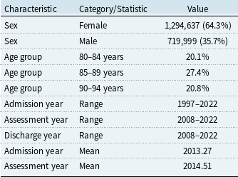
Selected demographic and temporal characteristics

Table 1. Long description
The table presents selected demographic and temporal characteristics. It has 10 rows and 3 columns. The columns are labeled Characteristic, Category/Statistic, and Value. The table includes data on sex, age group, admission year, assessment year, and discharge year. For sex, there are 1,294,637 females (64.3%) and 719,999 males (35.7%). Age groups include 80-84 years (20.1%), 85-89 years (27.4%), and 90-94 years (20.8%). Admission year ranges from 1997 to 2022 with a mean of 2013.27. Assessment year ranges from 2008 to 2022 with a mean of 2014.51. Discharge year ranges from 2008 to 2022.
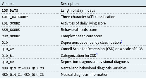
For the year variables, admission year refers to the year in which a resident entered residential aged care and may precede 2008. Assessment year refers to the year in which the recorded ACFI assessment was conducted.Footnote 1 Discharge year denotes the year in which the resident exited care or was formally recorded as discharged. Table 1 presents selected summary statistics for the main demographic and temporal characteristics. Table 2 outlines the information of outcome, assessment, depression, and other diagnostic variables.
Summary of key outcome and assessment variables

Table 2. Long description
A table with two columns and twelve rows. The columns are labeled ‘Variable’ and ‘Description’. Row 1: Variable, LOS_DAYS; Description, Length of stay in days. Row 2: Variable, ACFI_CATEGORY; Description, Three-character ACFI classification. Row 3: Variable, ADL_SCORE; Description, Activities of daily living score. Row 4: Variable, BEH_SCORE; Description, Behavioral needs score. Row 5: Variable, CHC_SCORE; Description, Complex health care score. Row 6: Variable, Q10; Description, Depression/dependency classification. Row 7: Variable, Q10_A2; Description, Cornell Scale for Depression (CSD) on a scale of 0-38. Row 8: Variable, Q10_R1; Description, Categorization for CSD. Row 9: Variable, Q10_R2; Description, Depression diagnosis/provisional diagnosis. Row 10: Variable, MBD_Q13_C1-MBD_Q13_C3; Description, Mental and behavioral diagnosis variables. Row 11: Variable, MED_Q14_C1-MED_Q14_C3; Description, Medical diagnosis information.
Overall, the data offer a rich and comprehensive basis for analyzing length of stay in residential aged care. Their main strengths are the large sample size, the long period of coverage, and the breadth of resident-level assessment and diagnosis information.
2.2 Assessment, depression, and diagnostic variables construction
This subsection describes the construction of the assessment, depression, and diagnosis variables used in the empirical analysis. We derive these variables from the ACFI assessment items, the Question 10 depression appraisal, and the diagnosis fields in Questions 13 and 14.
2.2.1 Question 10-related variables
Under the ACFI framework, Question 10 belongs to the Behavior domain and records information related to depression and dysthymia (Australian Government Department of Health, 2020). The raw data contain six Question 10 variables: Q10, Q10_A1, Q10_A2, Q10_A3, Q10_R1, and Q10_R2. Q10 is the rating from A to D, reflecting the dependence symptoms associated with depression and dysthymia. Additionally, Q10_A2 records the CSD score on a 0 to 38 scale while Q10_A1 indicates whether the CSD assessment was undertaken, Q10_A3 records whether supporting clinical information was provided, Q10_R1 classifies the CSD score of Q10_A2 into four categories,Footnote 4 Q10_R2 captures diagnosis or provisional diagnosis status. Here, Q10 is the main variable which combines Q10_R1 and Q10_R2 to produce the ACFI rating for chronic mood disturbance. Therefore, these six Question 10 variables can be summarized and extracted into two Question 10 measures for the analysis. First, we define CSD as the continuous depression measure given by Q10_A2. Second, we define CMD as the categorical measure of chronic mood disturbance given by Q10. This construction preserves both the raw severity information from the Cornell scale and the broader ACFI classification of mood disturbance.
2.2.2 Question 13-related variables
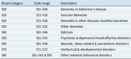
Question 13 records mental and behavioral diagnosis (MBD) information. It contains three fields, MBD_Q13_C1, MBD_Q13_C2, and MBD_Q13_C3, which allow up to three mental or behavioral diagnoses to be recorded in descending order of relevance to care needs, with C1 denoting the primary diagnosis, C2 the secondary diagnosis, and C3 the tertiary diagnosis (Australian Government Department of Health, 2020). These diagnosis codes fall within the ACFI MBD code range 500–599. Table 3 summarizes the corresponding broad code groups.
Mental and behavioral diagnosis code

Table 3. Long description
The table categorizes mental and behavioral diagnosis codes into broad categories with corresponding code ranges and descriptions. It has four columns: Broad category, Code range, and Description. The table contains eight rows with the following data: Row 1: Broad category, 500; Code range, 501-504; Description, Dementia in Alzheimer’s disease. Row 2: Broad category, 510; Code range, 511-516; Description, Vascular dementia. Row 3: Broad category, 520; Code range, 521-526; Description, Dementia in other diseases classified elsewhere. Row 4: Broad category, 530; Code range, 531-532; Description, Other dementia. Row 5: Broad category, 540; Code range, 541-544; Description, Delirium. Row 6: Broad category, 550; Code range, 551-553; Description, Psychoses & depression/mood affective disorders. Row 7: Broad category, 560; Code range, 561-564; Description, Neurotic, stress-related & somatoform disorders. Row 8: Broad category, 570; Code range, 571-572; Description, Intellectual & developmental disorders. Row 9: Broad category, 580; Code range, 581-583 & 599; Description, Other mental & behavioral disorders.
To obtain an empirically tractable diagnosis measure, we collapse the raw MBD codes into three broad groups: Organic & Cognitive Disorders (501–544), Psychotic & Mood Disorders (551–553), and Other Mental & Behavioral Disorders (561–599). We then aggregate information across C1, C2, and C3 to identify whether each diagnosis group is present for a resident. This procedure yields an eight-category variable, denoted by MBD: No Diagnosis, Other Only, Mood Only, Mood & Other, Organic Only, Organic & Other, Organic & Mood, and All Disorders.
2.2.3 Question 14-related variables
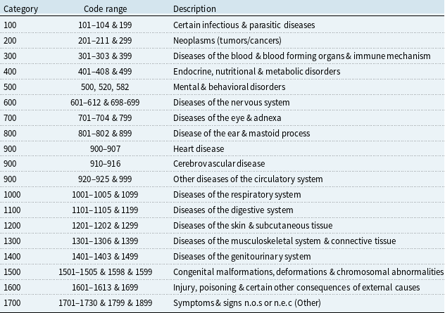
Question 14 records medical diagnosis information. This contains three fields, MED_Q14_C1, MED_Q14_C2, and MED_Q14_C3, which again record up to three diagnoses in descending order of relevance to care needs. The corresponding diagnosis codes span the broader ACFI medical diagnosis ranges outside the MBD block. Table 4 summarizes the main code groups.
Medical diagnosis code

Table 4. Long description
A table categorizing medical diagnosis codes and their descriptions. The table has three columns: Category, Code range, and Description. It contains 18 rows, each representing a different category of medical diagnosis codes. Row 1: Category, 100; Code range, 101-104 & 199; Description, Certain infectious & parasitic diseases. Row 2: Category, 200; Code range, 201-211 & 299; Description, Neoplasms (tumors/cancers). Row 3: Category, 300; Code range, 301-303 & 399; Description, Diseases of the blood & blood forming organs & immune mechanism. Row 4: Category, 400; Code range, 401-408 & 499; Description, Endocrine, nutritional & metabolic disorders. Row 5: Category, 500; Code range, 500, 520, 582; Description, Mental & behavioral disorders. Row 6: Category, 600; Code range, 601-612 & 698-699; Description, Diseases of the nervous system. Row 7: Category, 700; Code range, 701-704 & 799; Description, Diseases of the eye & adnexa. Row 8: Category, 800; Code range, 801-802 & 899; Description, Disease of the ear & mastoid process. Row 9: Category, 900; Code range, 900-907; Description, Heart disease. Row 10: Category, 900; Code range, 910-916; Description, Cerebrovascular disease. Row 11: Category, 900; Code range, 920-925 & 999; Description, Other diseases of the circulatory system. Row 12: Category, 1000; Code range, 1001-1005 & 1099; Description, Diseases of the respiratory system. Row 13: Category, 1100; Code range, 1101-1105 & 1199; Description, Diseases of the digestive system. Row 14: Category, 1200; Code range, 1201-1202 & 1299; Description, Diseases of the skin & subcutaneous tissue. Row 15: Category, 1300; Code range, 1301-1306 & 1399; Description, Diseases of the musculoskeletal system & connective tissue. Row 16: Category, 1400; Code range, 1401-1403 & 1499; Description, Diseases of the genitourinary system. Row 17: Category, 1500; Code range, 1501-1505 & 1598 & 1599; Description, Congenital malformations, deformations & chromosomal abnormalities. Row 18: Category, 1600; Code range, 1601-1613 & 1699; Description, Injury, poisoning & certain other consequences of external causes. Row 19: Category, 1700; Code range, 1701-1730 & 1799 & 1899; Description, Symptoms & signs n.o.s or n.e.c (Other).
Given that the core predictive variables of this study are functional status (ADL), behavioral symptoms (BEH), and comprehensive care needs (CHC), medical diagnoses are primarily included as adjustment covariates for baseline health status in the model. Based on clinical prevalence distribution and statistical stability considerations, we classify the raw medical diagnosis codes into three broad groups: Cancer (200–299), Diseases of the Circulatory System (900–999), and Other Disease (all remaining medical diagnosis codes). Circulatory diseases and cancer are not only the most prevalent in the long-term care population, but also represent the primary disease burden affecting survival prognosis in the elderly. The prevalence of each remaining diagnostic category is less than 5%. Classifying them separately would lead to sparse data issues and highly unstable risk estimates. Therefore, consolidating these low-frequency categories into an ”Other” category ensures both the computational feasibility of the model within the large-scale survival forest algorithm and the statistical reliability of risk estimates within each stratum.
By doing this, we construct a grouped diagnosis variable for empirical analysis as with Question 13. Specifically, We then combine information across C1, C2, and C3 to determine whether each group is present. This produces an eight-category variable, denoted by MED: No Diagnosis, Other Only, Circulatory Only, Cancer Only, Circulatory & Other, Cancer & Other, Cancer & Circulatory, and Cancer & Circulatory & Other.
2.2.4 ACFI category variables
In addition to the depression variables above, we construct continuous and categorical representations for each of the three core ACFI domains. The continuous measures are given directly by the recorded domain scores: ADL_SCORE, BEH_SCORE, and CHC_SCORE, which we denote by ADL, BEH, and CHC, respectively. The categorical measures are derived from the three-character ACFI_CATEGORY, where the first character records the level for ADL, the second character records the level for Behavior, and the third character records the level for CHC. Each domain is classified into four levels: Nil (N), Low (L), Medium (M), and High (H).
Accordingly, we define ADL_CAT as the first character of ACFI_CATEGORY, BEH_CAT as the second character, and CHC_CAT as the third character. This yields, for each domain, a continuous score that preserves within-category variation and a categorical level that reflects the discrete ACFI classification.
2.3 Data pre-processing
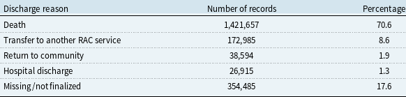
Following Zhang et al. (Reference Zhang, Shi and Huang2023), we define death as the event of interest and treat all other discharge outcomes as right-censored observations. Table 5 reports the distribution of discharge reasons in the raw data.
Distribution of discharge outcomes

Table 5. Long description
The table presents the distribution of discharge outcomes, detailing the reasons for discharge, the number of records, and the corresponding percentages. It has four columns: Discharge reason, Number of records, and Percentage. The table includes the following data: Row 1: Death, 1,421,657, 70.6 percent. Row 2: Transfer to another RAC service, 172,985, 8.6 percent. Row 3: Return to community, 38,594, 1.9 percent. Row 4: Hospital discharge, 26,915, 1.3 percent. Row 5: Missing/not finalized, 354,485, 17.6 percent.
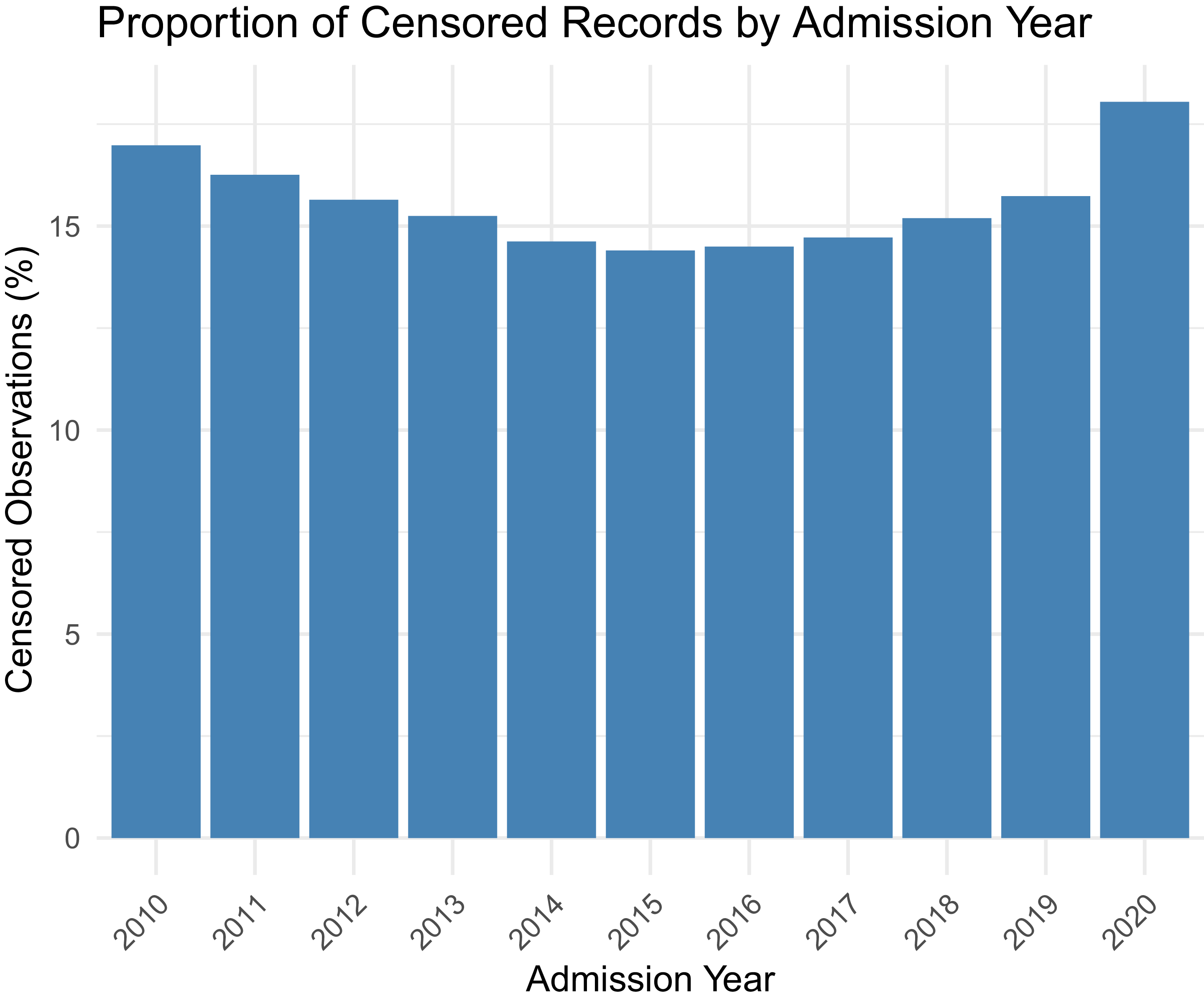
Proportion of right-censored records by admission year.

Consistent with Zhang et al. (Reference Zhang, Shi and Huang2023) and Fracalossi et al. (Reference Fracalossi, Zhang, Lee and Shi2025), we adopt the following steps to pre-process our dataset. First, we exclude residents aged 1–49 at assessment. This group accounts for only 0.27% of the raw sample and is not representative of the mainstream residential aged care population. Second, because age at admission is not directly observed, we estimate the admission age group using age at assessment together with admission year and assessment year, following the midpoint approach under a uniform distribution assumption in Zhang et al. (Reference Zhang, Shi and Huang2023). Third, we exclude the open-ended age group 100+, which represents a small share of the data, around 0.9%, and is not directly comparable with the closed five-year age intervals used for the remaining sample. Fourth, to limit the influence of extreme observations, we trim the bottom and top 2.5% of the length-of-stay distribution. This removes observations with length of stay below 0.6 months and above 129 months. Finally, we restrict admission year to the period 2000–2022 and remove observations with missing values in the variables required for analysis.
After these steps, the final analytic sample contains 1,583,368 observations. The response variable is LOS, measured in months, together with the event indicator censor. The covariates used in the analysis are AGE, YEAR (admission year), SEX, ADL, ADL_CAT, BEH, BEH_CAT, CHC, CHC_CAT, CSD, CMD, MBD, and MED.
2.4 Preliminary analysis
This section provides a brief descriptive overview of the data and highlights several broad empirical patterns. One of most important features of the data is the presence of right-censored records. Figure 1 presents the proportion of right-censored records by admission year for the period 2010–2020. The censoring proportion fluctuates around 15%, with an initial decline, a stable trough, and a slight increase recently. It should be noted that the proportion of uncensored records differs from the proportion of deaths in Table 5, as observations with missing values and those from certain age groups were removed. Despite the mechanical truncation of observed stays for cohorts closer to the end of the observation period, the overall censoring rate does not exhibit a substantial increase. However, this does not eliminate the concern that simple average uncensored lengths of stay are misleading. Even with a stable censoring proportion, the longest stays in later cohorts are systematically more likely to be censored (and thus excluded from average uncensored calculations), because the maximum possible follow-up time is mechanically shorter for these cohorts. This figure therefore provides important context for interpreting the Kaplan–Meier (KM) (Kaplan & Meier, Reference Kaplan and Meier1958) estimates that follow.
Figure 2 presents KM survival curves stratified by admission year (2010–2020), showing the proportion of residents remaining in care over time (in months). Several patterns emerge. First, the KM-estimated survival curves for later cohorts (post-2016) drop more steeply in the early months following admission compared with earlier cohorts, suggesting a shortening of length of stay in more recent years. Second, the gap between the KM curves and the naive estimates based on uncensored records are close because the proportion of censored records is just around 15%, however, this does not mean that the difference can be ignored. Hence, it is important to take the censorship into account. Third, the median survival time provides a clear summary, the medians length of stay of later years are declining. This decline is consistent with broader trends documented in the Australian residential aged care sector, where average length of stay has decreased from approximately 34–35 months (2007–2008 to 2010–2011) to around 30 months (2016–2017 to 2017–2018) and is projected to continue declining (Zhang et al., Reference Zhang, Shi and Huang2023).
Figure 3 presents KM survival curves stratified by key resident characteristics, SEX, AGE, ADL_CAT, BEH_CAT, CHC_CAT, CMD, MBD, and MED. This allows for direct comparison of survival trajectories across groups using the 50% threshold (median length of stay). The figures reveal considerable heterogeneity across resident groups. The survival probability differs persistently by sex, with females tending to remain in care longer than males. Differences are also evident across age groups, with older residents generally experiencing shorter stays, consistent with their higher mortality risk. In addition, the length of stay varies across ACFI domain levels, mood disturbance categories, and diagnosis profiles. The visual patterns further suggest that the association between care needs and length of stay is not uniform across domains. Higher levels of ADL and CHC are generally associated with shorter stays, whereas the relationships for BEH and CMD are not that obvious. These differences provide preliminary evidence that the relationship between resident characteristics and length of stay is heterogeneous and unlikely to be adequately captured by simple linear effects.
Kaplan–Meier estimates of the survival curve for residents by admission year.

Figure 2 Long description
Panel A: A line graph depicting survival probability in percent on the vertical axis and length of stay in months on the horizontal axis. The graph includes multiple lines representing different admission years from 2010 to 2020. Solid lines indicate total survival probability, while dashed lines indicate uncensored data. Each line shows a downward trend, indicating a decrease in survival probability over time. The lines for different years vary in their steepness and starting points, reflecting differences in survival probabilities based on the admission year.
Kaplan–Meier estimates of the survival curve for residents with different characteristics.

We next examine how the ACFI domain levels vary across diagnosis profiles. Figure 4 reports the distribution of ADL, BEH, and CHC levels within each category of MBD and MED. The figure suggests that more severe MBD profiles are associated with higher assessed needs in ADL and, more clearly, in BEH. By contrast, the distribution of CHC levels appears less sharply differentiated across MBD categories. For MED, the distributions of ADL, BEH, and CHC appear comparatively more stable across diagnosis groups. These descriptive patterns indicate that the diagnosis variables are related to the ACFI assessment profiles, although the strength and form of the relationship differ across domains.
Proportions of ADL, BEH, and CHC levels by categories of MBD and MED.

Figure 4 Long description
Panel A: A vertical bar graph shows the distribution of levels of ADL by MBD diagnoses. The x-axis represents different MBD diagnoses, and the y-axis represents the percentage. The legend indicates levels N, L, M, and H. Panel B: A vertical bar graph shows the distribution of levels of BEH by MBD diagnoses. The x-axis represents different MBD diagnoses, and the y-axis represents the percentage. The legend indicates levels N, L, M, and H. Panel C: A vertical bar graph shows the distribution of levels of CHC by MBD diagnoses. The x-axis represents different MBD diagnoses, and the y-axis represents the percentage. The legend indicates levels N, L, M, and H. Panel D: A vertical bar graph shows the distribution of levels of ADL by MED diagnoses. The x-axis represents different MED diagnoses, and the y-axis represents the percentage. The legend indicates levels N, L, M, and H. Panel E: A vertical bar graph shows the distribution of levels of BEH by MED diagnoses. The x-axis represents different MED diagnoses, and the y-axis represents the percentage. The legend indicates levels N, L, M, and H. Panel F: A vertical bar graph shows the distribution of levels of CHC by MED diagnoses. The x-axis represents different MED diagnoses, and the y-axis represents the percentage. The legend indicates levels N, L, M, and H.
Overall, the exploratory analysis highlights three key features of the data. First, length of stay varies substantially across demographic, assessment, and diagnosis groups. Second, the diagnosis variables are associated with distinct ACFI profiles, particularly for mental and behavioral diagnoses. Third, the visual patterns indicate heterogeneity across resident groups and potential nonlinearity in the relationship between covariates and length of stay. These features suggest the need for a more sophisticated statistical framework capable of accommodating such complexities.
2.5 Preliminary tests
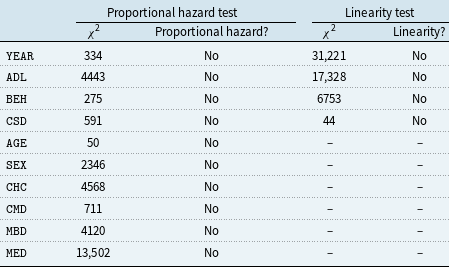
We begin by examining three features of the data that are central to model choice: the proportional hazards assumption, the functional form of continuous covariates, and the dependence structure among predictors. For the proportional hazards assumption, we use the test of Grambsch and Therneau (Reference Grambsch and Therneau1994). For linearity, we use the test implemented in Harrell et al. (Reference Harrell, Harrell and Hmisc2017). The resulting test statistics are reported in Table 6.
Test statistics on proportional hazard and linearity of variables

Table 6. Long description
A table with two columns: Proportional hazard test and Linearity test. Each column has two sub-columns: chi-squared values and results. The table has 10 rows labeled with different variables: YEAR, ADL, BEH, CSD, AGE, SEX, CHC, CMD, MBD, MED. Each row contains chi-squared values and results for proportional hazard and linearity tests. All variables show ‘No’ for both proportional hazard and linearity.
It is clear that the results provide little support for a standard Cox specification. The proportional hazards assumption is rejected for all variables considered. In addition, the continuous covariates do not exhibit simple linear effects. Taken together, these findings suggest that the relationship between resident characteristics and length of stay is more complex than can be adequately captured by a conventional proportional hazards model with linear terms.
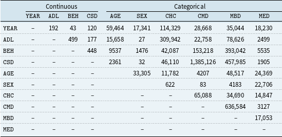
Next, we examine the dependence structure among the covariates. Table 7 reports the corresponding test statistics. Following the measurement scale of each variable pair, we use Pearson’s correlation test for pairs of continuous variables, the Kruskal–Wallis test for continuous and categorical pairs, and Pearson’s chi-squared test for pairs of categorical variables. Overall, our results indicate strong dependence across the covariates.
Test statistics of independence tests among variablesFootnote 5

Table 7. Long description
The table presents test statistics of independence tests among variables, divided into continuous and categorical sections. It includes 10 rows and 11 columns. The columns are labeled as follows: YEAR, ADL, BEH, CSD, AGE, SEX, CHC, CMD, MBD, and MED. Each row represents a variable and its corresponding test statistics with other variables. Row 1: YEAR, 192, 43, 120, 59,464, 17,341, 114,329, 28,668, 35,044, 18,230. Row 2: ADL, 499, 177, 15,658, 27, 309,942, 22,758, 78,626, 2499. Row 3: BEH, 448, 9537, 1476, 42,087, 153,218, 393,042, 5535. Row 4: CSD, 2361, 32, 46,110, 1,385,126, 457,985, 1905. Row 5: AGE, 33,305, 11,782, 4207, 48,517, 24,369. Row 6: SEX, 622, 83, 4183, 22,706. Row 7: CHC, 65,088, 34,690, 14,847. Row 8: CMD, 636,584, 3127. Row 9: MBD, 17,053. Row 10: MED.
In summary, the preliminary tests point to three important features of the data: departures from proportional hazards, nonlinear covariate effects, and substantial dependence among predictors. These findings support the use of a more flexible survival modeling framework and provide empirical justification for the AORSF adopted in this study, which is to be discussed in Section 3.
3. Methodology
As explained in Section 2, the primary outcome of interest is length of stay in residential aged care, which is observed as a right-censored time-to-event variable. This section describes the empirical methodology used to model length of stay by incorporating the full set of explanatory variables.
Let
 $T_i$
denote the observed stay duration for resident
 $i$
, measured in months, and let
 $\delta _i$
be the event indicator, where
 $\delta _i=1$
if the resident dies and
 $\delta _i=0$
otherwise. For a covariate vector
 $\mathbf{x}_i$
, our primary target is the conditional survival function
 \begin{equation*} S(t \mid \mathbf{x}_i)=\Pr (T_i\gt t \mid \mathbf{x}_i), \end{equation*}
which characterizes the full distribution of remaining stay duration given resident characteristics.
A natural starting point for survival analysis is the Cox proportional hazards model (Cox, Reference Cox1972). However, its usefulness depends on a proportional hazards structure and a sufficiently parsimonious functional form. When the proportional hazards assumption fails, the estimated regression effects may be difficult to interpret and may not represent stable effects over time (Dunkler et al., Reference Dunkler, Schemper and Heinze2010; Xu & O’Quigley, Reference Xu and O’Quigley2000). Weighted Cox regression and related extensions can partially address this issue, while stratification can accommodate some forms of non-proportionality for categorical variables (Dunkler et al., Reference Dunkler, Ploner, Schemper and Heinze2018; Schemper et al., Reference Schemper, Wakounig and Heinze2009). However, these approaches still require specifications of nonlinear terms, time-varying effects, and interaction structures in advance. In large administrative care datasets, where demographic characteristics, ACFI scores, depression indicators, and diagnosis variables may interact in complicated ways, such specification can become restrictive. In the Australian residential aged care setting, Zhang et al. (Reference Zhang, Shi and Huang2023) address these issues using an extended Cox framework. Adopting this approach requires explicit modeling decisions regarding stratification and nonlinear adjustment and is not well suited to our sample size.Footnote 6
These considerations motivate a more flexible survival modeling framework. A natural candidate is the random survival forest (RSF), which extends the random forest approach of Breiman (Reference Breiman2001) to censored time-to-event data (Ishwaran et al., Reference Ishwaran, Kogalur, Blackstone and Lauer2008). Relative to Cox-type models, RSF is particularly well suited to our setting for two reasons. First, RSF recursively partitions the covariate space and can therefore capture heterogeneous relationships across resident groups without requiring interactions or subgroup structures to be specified in advance. This is especially important in our setting, where demographic characteristics, ACFI assessments, depression indicators, and diagnosis variables may interact in complex ways. Second, RSF accommodates nonlinear covariate effects and does not rely on the proportional hazards assumption. This is therefore well suited to the empirical patterns identified in Section 2, including heterogeneity across groups and potentially nonlinear associations between resident characteristics and length of stay. Compared with the approach used by Fracalossi et al. (Reference Fracalossi, Zhang, Lee and Shi2025), RSF retains the survival structure of the data and directly accounts for censoring. Compared with the extended Cox model in Zhang et al. (Reference Zhang, Shi and Huang2023), it allows for more flexible dependence among predictors and can produce robust estimates of the conditional survival function. The ability of RSF to accommodate nonlinearity, covariate dependence, and departures from proportional hazards is also well recognized in the literature (Birolo et al., Reference Birolo, Rossi, Sartori, Rollo, Fariselli and Sanavia2025; Cui et al., Reference Cui, Zhu, Zhou and Kosorok2022).
In this paper, we adopt the AORSF of Jaeger et al. (Reference Jaeger, Welden, Lenoir, Speiser, Segar, Pandey and Pajewski2024). Relative to standard RSF, which uses axis-aligned splits based on a single predictor at each node, oblique forests split on linear combinations of predictors. This is attractive in our sample because the covariates are strongly associated by construction and include overlapping continuous and categorical measures of care needs, mood disturbance, and diagnosis burden. Prior work shows that oblique forests can improve predictive performance over axis-based forests under such cases with correlated predictors (Jaeger et al., Reference Jaeger, Long, Long, Sims, Szychowski, Min, Mcclure, Howard and Simon2019; Menze et al., Reference Menze, Kelm, Splitthoff, Koethe and Hamprecht2011). Recent evidence further suggests that oblique survival forests perform well in moderate-to-large samples, which is also related to our case (Berkowitz et al., Reference Berkowitz, Altman and Loughin2024).
Formally, let
 \begin{equation*} \mathcal{D}_n=\{(T_i,\delta _i,\mathbf{x}_i)\}_{i=1}^n \end{equation*}
denote the observed sample. AORSF grows an ensemble of survival trees by recursively partitioning the covariate space. At each non-terminal node, the split direction is determined by an oblique combination of predictors. In the accelerated implementation of Jaeger et al. (Reference Jaeger, Welden, Lenoir, Speiser, Segar, Pandey and Pajewski2024), this linear combination is obtained using a one-step Newton scoring update based on the Cox partial likelihood, which substantially reduces computational cost relative to earlier oblique survival forests. Each tree yields an estimated survival function for observations falling in the relevant terminal node, and the forest prediction is the average of the tree-level survival estimates:
 \begin{equation*} \widehat {S}(t \mid \mathbf{x})=\frac {1}{B}\sum _{b=1}^{B}\widehat {S}_b(t \mid \mathbf{x}), \end{equation*}
where
 $B$
is the number of trees and
 $\widehat {S}_b(t \mid \mathbf{x})$
is the survival estimate from tree
 $b$
.
Model performance was evaluated using OOB estimates to avoid overfitting. The primary metric was Harrell’s C-index (Harrell et al., Reference Harrell, Califf, Pryor, Lee and Rosati1982), which measures the model’s ability to correctly rank the risk of residents; higher values indicate better discrimination between those who exit care earlier and those who remain longer. The aorsf package uses the OOB C-index as its default evaluation metric for variable importance computation and model tuning. For benchmark comparison, a Cox proportional hazards model with the same set of covariates was fitted and evaluated using 100-repetition bootstrap cross-validation.
4. Results
This section presents the empirical results. We first evaluate the predictive performance against the benchmark model, Cox proportional hazards model in Zhang et al. (Reference Zhang, Shi and Huang2023), using bootstrap cross-validation (100 repetitions). Based on the AORSF model that we fit, we then report the main findings from the AORSF specification and examine how the importance of key predictors varies across resident groups and care profiles.
4.1 Predictive performance evaluation
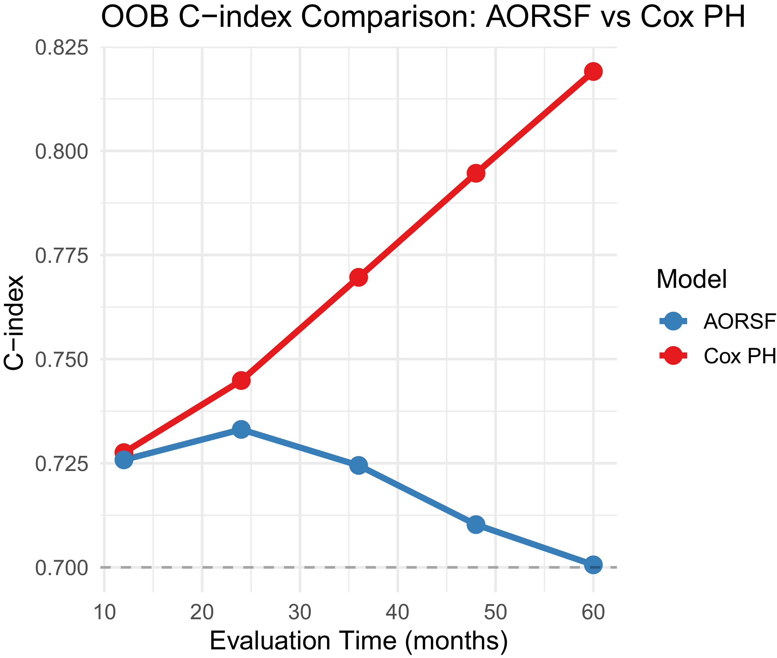
The predictive performance of the AORSF against the Cox proportional hazards model is displayed in Figure 5. The OOB Harrell’s C-index for AORSF ranged from 0.70 to 0.72 across the five evaluation time points, indicating stable discrimination throughout the follow-up period. This stability is a characteristic of the ensemble learning approach, which does not rely on the proportional hazards assumption. For comparison, the Cox proportional hazards model showed an increasing C-index from 0.73 at 12 months to 0.82 at 60 months, consistent with the proportional hazards assumption becoming more pronounced over longer follow-up. This pattern reflects the fundamental difference between the two modeling approaches: the parametric Cox model can amplify long-term discrimination under its assumptions, while the non-parametric AORSF provides stable, robust predictions without such assumptions.
Out-of-bag Harrell’s C-index comparison.

Bar plot of variable importance.

4.2 Baseline results: full-sample variable importance
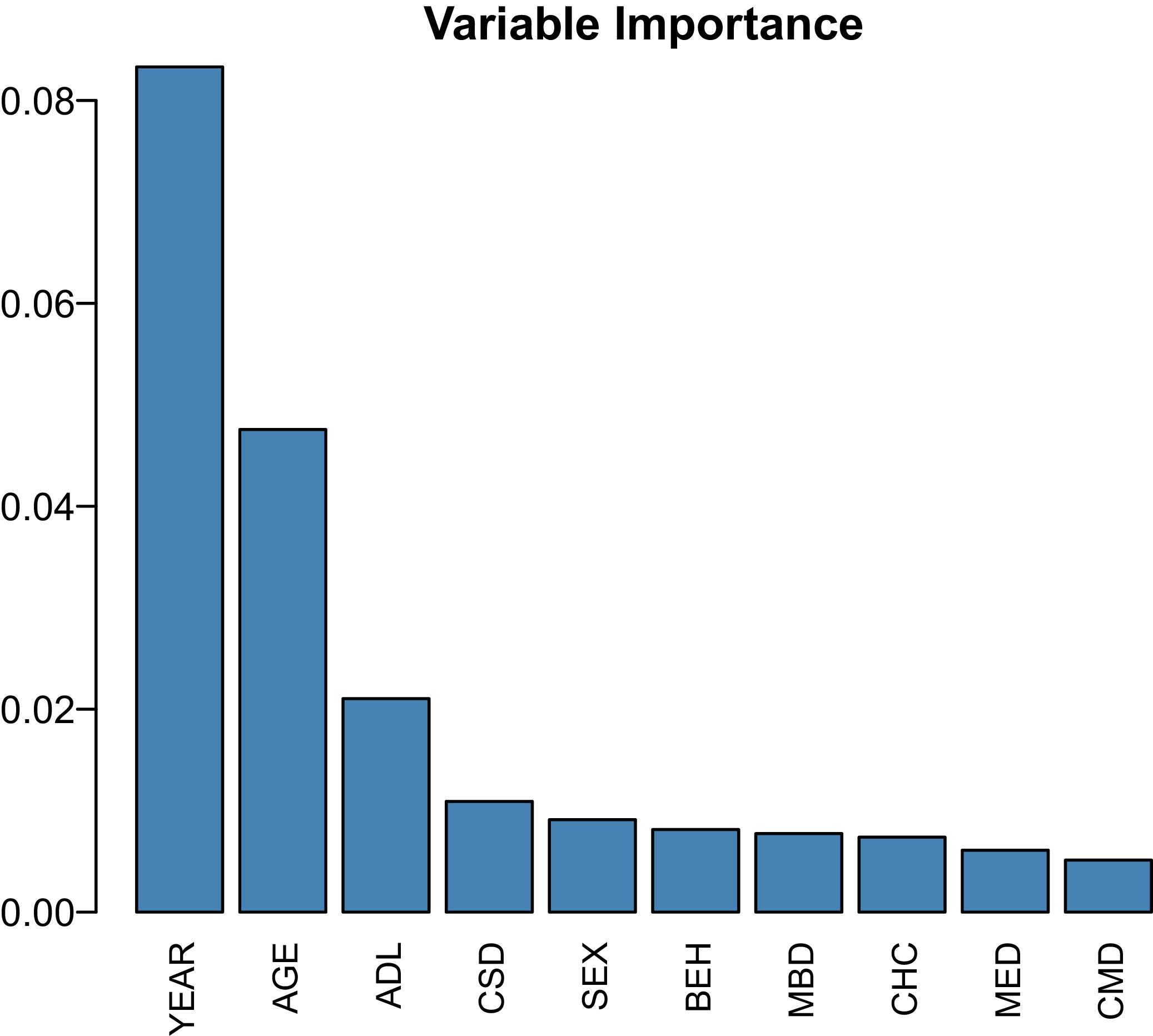
We present the baseline findings from the AORSF model in this section. We used permutation variable importance as implemented in the aorsf package. Figure 6 reports the variable importance ranking for the full sample. Three variables emerge as the most important predictors: YEAR, AGE, and ADL. This suggests that the intensity of residents’ daily care needs, as measured by ADL, is a critical determinant of length of stay in residential aged care, alongside the expected effects of admission year and admission age.
Beyond these leading predictors, the full-sample ranking also highlights the importance of mental and behavioral information. In particular, CSD emerges as one of the most influential variables, followed by SEX and BEH. The prominence of CSD is especially notable, as it suggests that depression-related symptoms contain substantial predictive information for length of stay even after accounting for age, admission year, and physical dependency. By contrast, the broader diagnosis indicators MBD and MED, together with CHC and CMD, appear lower in the overall ranking. Taken together, this suggests that detailed assessment-based measures, particularly those related to function and mood, are more informative than broader grouped diagnosis categories.
A further variable-selection exercise based on the optimal OOB prediction accuracy yields a parsimonious set of predictors consisting of YEAR, AGE, ADL, CSD, SEX, and BEH. This reduced set is informative in two respects. First, it confirms the central role of admission year, age, and functional dependency in explaining length of stay. Second, it shows that mental and behavioral variables remain important even after applying a predictive selection criterion. In particular, both CSD and BEH are retained, which reinforces the view that mood and behavioral symptoms should not be treated as peripheral characteristics in modeling residential aged care trajectories.
Scree plot of interaction effects among covariates.

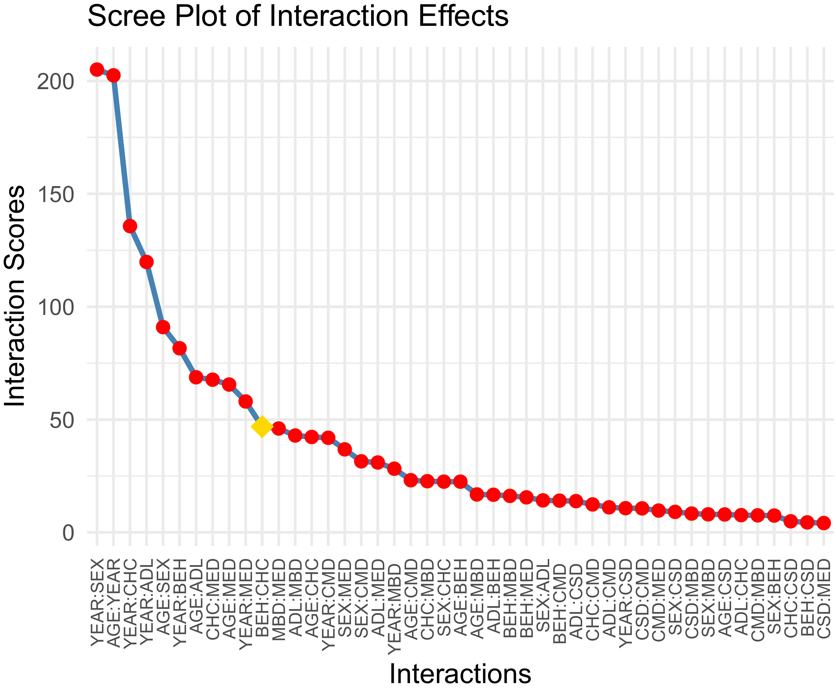
To complement the main-effect ranking, Figure 7 reports the interaction scores for all two-way combinations of covariates. The highest-ranked interactions are concentrated around YEAR and AGE, with particularly strong pairings involving SEX, CHC, ADL, BEH, and MED. This pattern suggests that admission year and age do not merely enter as dominant marginal predictors. Rather, they appear to influence the predictive role of other resident characteristics. In practical terms, the importance of care-need measures and diagnosis variables is likely to depend on when the resident entered care and how old the resident was at admission.
In summary, the baseline results deliver two main messages. First, the full-sample evidence points to a clear core set of predictors, centered on admission year, age, functional dependency, and depression-related symptoms. Second, the interaction structure indicates that these aggregate rankings are unlikely to be uniform across resident groups. This leaves clear room for a more detailed subsample analysis, which is undertaken in the next subsection.
4.3 Subsample analysis: heterogeneity across care profiles, admission year, and age
To examine the heterogeneity across residents more closely, we consider three dimensions of variation: care profiles defined by the ACFI domains, admission year, and age group. Across these dimensions, the main objective is to assess how the relative importance of the clinical and assessment variables changes across resident groups. For each subgroup analysis, we refitted the oblique RSF model independently on the respective subset and computed variable importance measures from that subset-specific model, rather than applying a global model fitted on the full sample. To assess the predictive contribution of each covariate, we used permutation variable importance as implemented in the aorsf package (Jaeger et al., Reference Jaeger, Long, Long, Sims, Szychowski, Min, Mcclure, Howard and Simon2019).
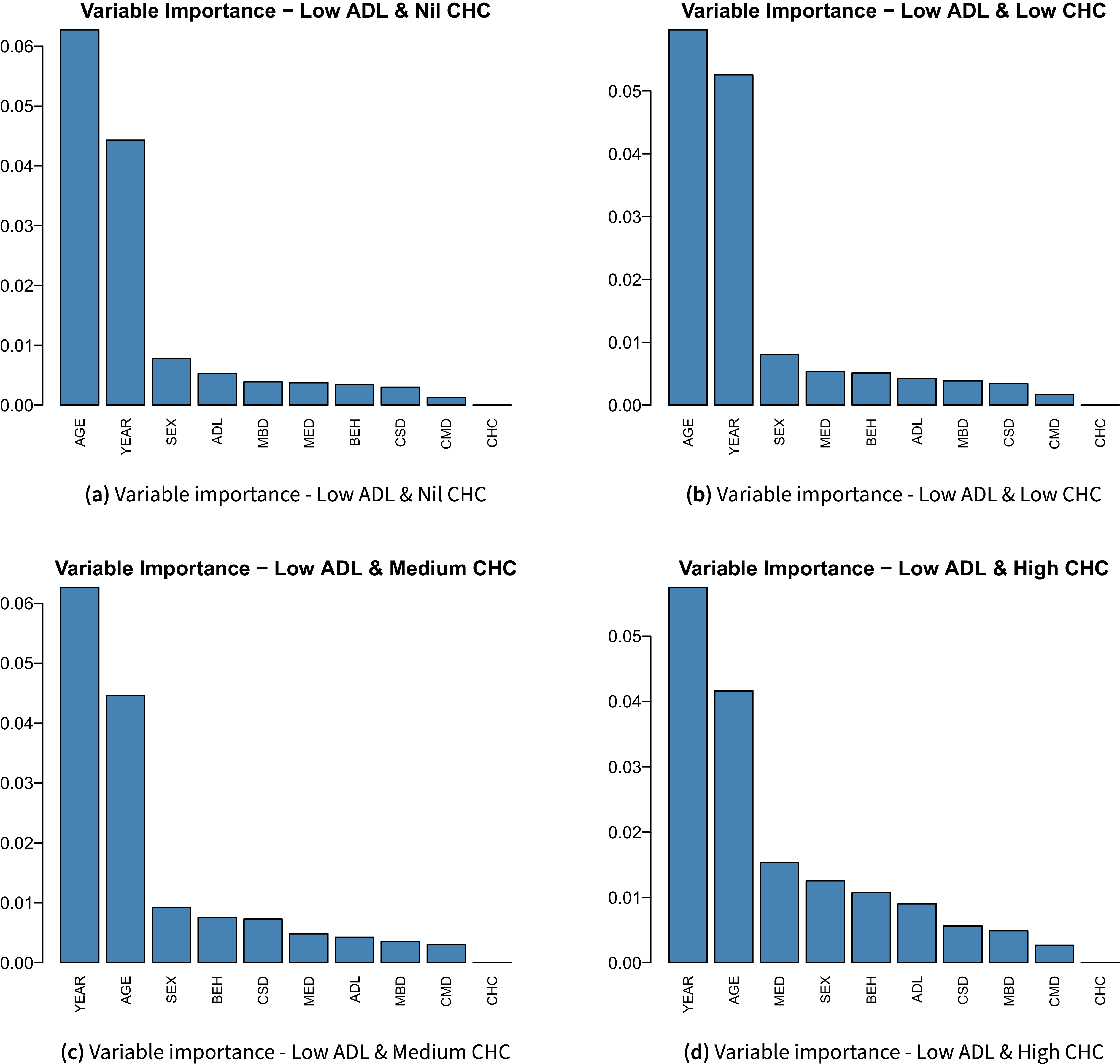
Variable importance in predicting LOS for different levels of CHC with nil level of ADL.

Variable importance in predicting LOS for different levels of CHC with low level of ADL.

Figure 9 Long description
Panel A: A vertical bar graph titled ‘Variable Importance - Low ADL & Nil CHC’ shows the importance of various variables in predicting length of stay. The x-axis lists variables such as AGE, YEAR, SEX, ADL, MBD, MED, BEH, CSD, CMD, and CHC. The y-axis represents variable importance ranging from 0.00 to 0.06. AGE and YEAR are the most important variables. Panel B: A vertical bar graph titled ‘Variable Importance - Low ADL & Low CHC’ shows the importance of various variables in predicting length of stay. The x-axis lists variables such as AGE, YEAR, SEX, MED, BEH, ADL, MBD, CSD, CMD, and CHC. The y-axis represents variable importance ranging from 0.00 to 0.06. AGE and YEAR are the most important variables. Panel C: A vertical bar graph titled ‘Variable Importance - Low ADL & Medium CHC’ shows the importance of various variables in predicting length of stay. The x-axis lists variables such as YEAR, AGE, SEX, BEH, CSD, MED, ADL, MBD, CMD, and CHC. The y-axis represents variable importance ranging from 0.00 to 0.06. YEAR and AGE are the most important variables. Panel D: A vertical bar graph titled ‘Variable Importance - Low ADL & High CHC’ shows the importance of various variables in predicting length of stay. The x-axis lists variables such as YEAR, AGE, MED, SEX, BEH, ADL, CSD, MBD, CMD, and CHC. The y-axis represents variable importance ranging from 0.00 to 0.06. YEAR and AGE are the most important variables.
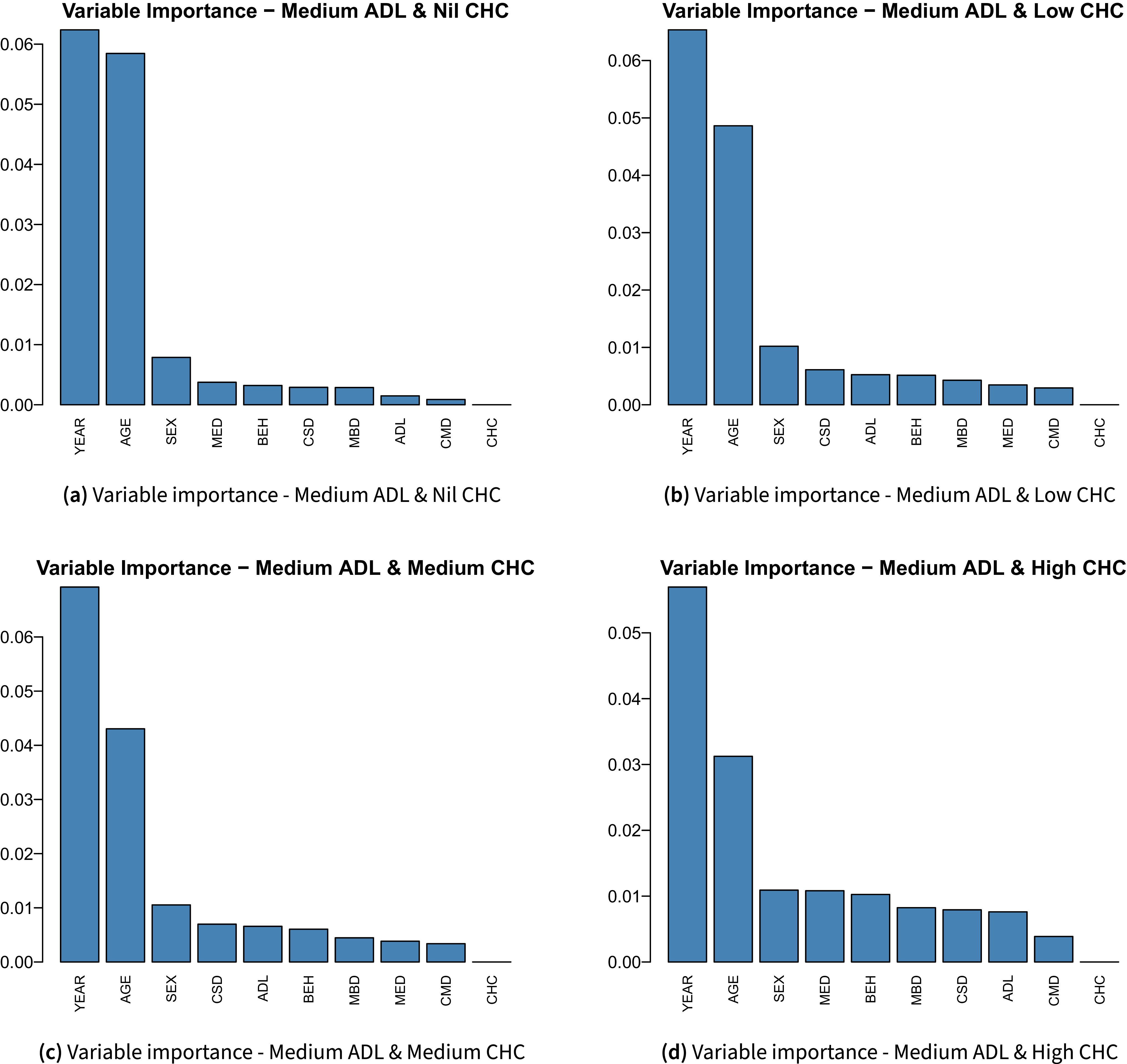
Variable importance in predicting LOS for different levels of CHC with medium level of ADL.

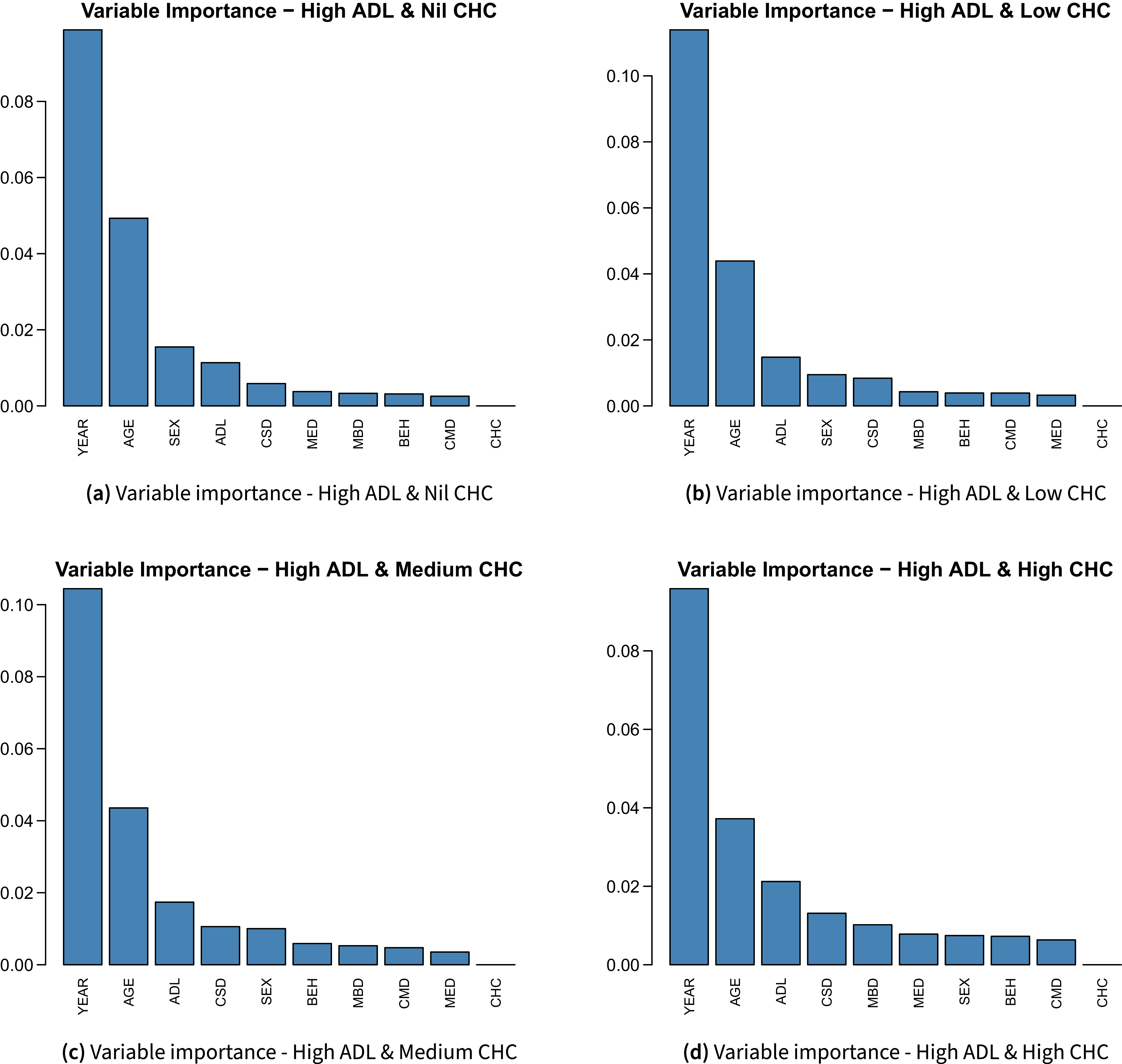
Variable importance in predicting LOS for different levels of CHC with high level of ADL.

Figure 11 Long description
Panel A: A vertical bar graph titled ‘Variable Importance - High ADL & Nil CHC’ shows the importance of various factors in predicting length of stay. The horizontal axis lists factors such as YEAR, AGE, SEX, ADL, CSD, MED, MBD, BEH, CMD, and CHC. The vertical axis represents the importance value ranging from 0.00 to 0.08. YEAR has the highest importance, followed by AGE, SEX, and ADL. Panel B: A vertical bar graph titled ‘Variable Importance - High ADL & Low CHC’ shows the importance of various factors in predicting length of stay. The horizontal axis lists factors such as YEAR, AGE, ADL, SEX, CSD, MBD, BEH, CMD, MED, and CHC. The vertical axis represents the importance value ranging from 0.00 to 0.10. YEAR has the highest importance, followed by AGE, ADL, and SEX. Panel C: A vertical bar graph titled ‘Variable Importance - High ADL & Medium CHC’ shows the importance of various factors in predicting length of stay. The horizontal axis lists factors such as YEAR, AGE, ADL, CSD, SEX, BEH, MBD, CMD, MED, and CHC. The vertical axis represents the importance value ranging from 0.00 to 0.10. YEAR has the highest importance, followed by AGE, ADL, and CSD. Panel D: A vertical bar graph titled ‘Variable Importance - High ADL & High CHC’ shows the importance of various factors in predicting length of stay. The horizontal axis lists factors such as YEAR, AGE, ADL, CSD, MBD, MED, SEX, BEH, CMD, and CHC. The vertical axis represents the importance value ranging from 0.00 to 0.10. YEAR has the highest importance, followed by AGE, ADL, and CSD.
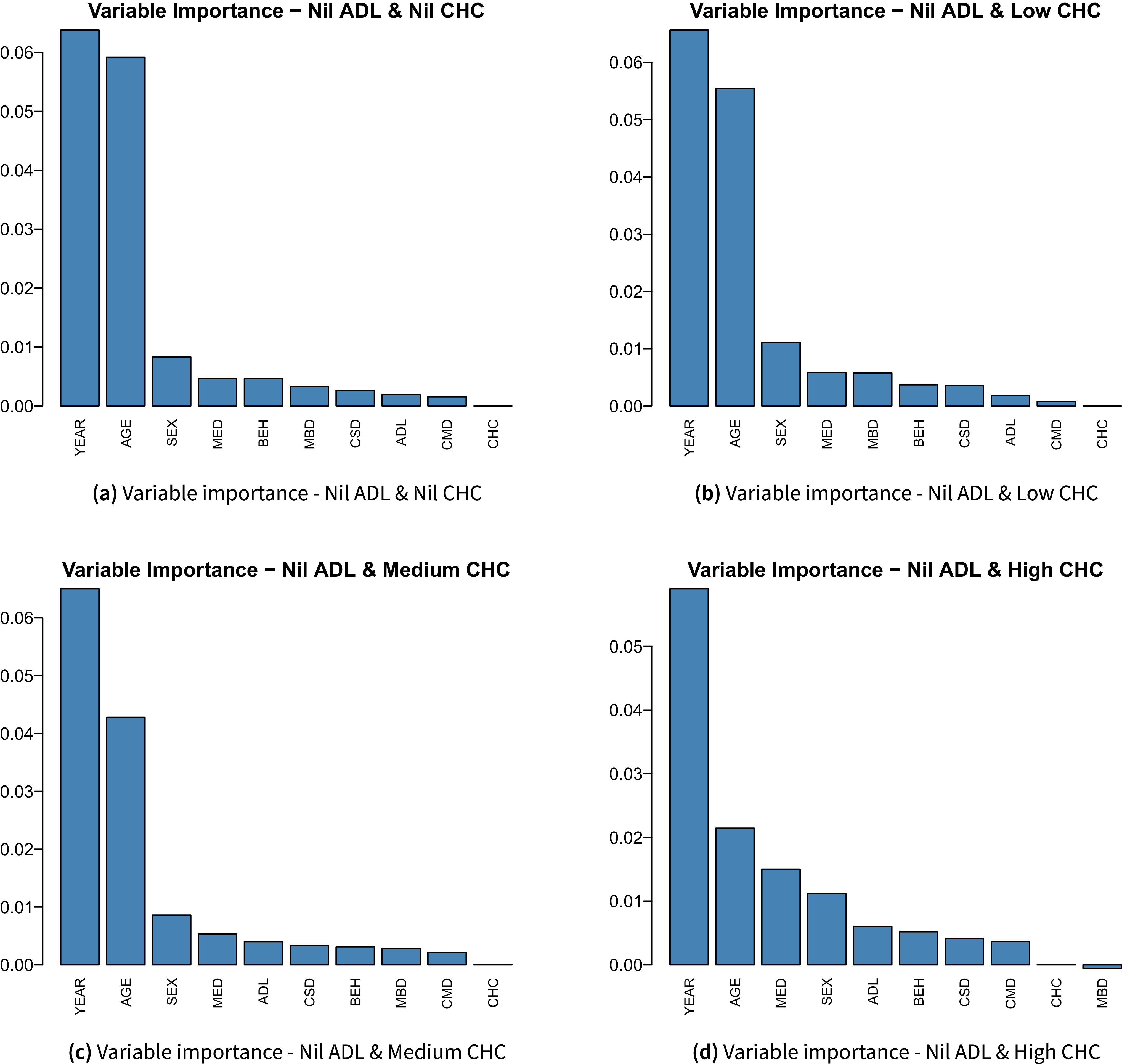
We begin with the ACFI-based subsample analysis. Figures 8–11 report variable-importance rankings across combinations of ADL and CHC levels. A consistent pattern across all panels is that YEAR and AGE remain among the most important predictors, as expected. The more informative heterogeneity therefore lies in the relative importance of the remaining covariates. When ADL is at the Nil or Low level, medical diagnosis burden, measured by MED, remains highly influential and becomes more prominent as CHC increases. In these lower-need strata, depression-related and behavioral variables appear in the rankings but do not consistently occupy the top positions. Their importance becomes more apparent only when CHC reaches at least the Medium level.
A different pattern emerges when ADL is at the Medium or High level. In these higher-need strata, depression-related and mental-behavioral variables become much more prominent. In particular, CSD moves into the upper tier of predictors and, in some cases, ranks ahead of broader diagnosis measures. A similar, although less uniform, pattern is observed for MBD and BEH. This tendency is strongest in the highest-need groups, especially when both ADL and CHC are high, where CSD and MBD stand out much more clearly than in the lower-need strata. Overall, Figures 8–11 suggest that as residents’ care needs intensify, predictive importance shifts away from broad medical burden alone and increasingly toward depression-related and mental-behavioral conditions.
Changes in ranks of variable importance by admission year.

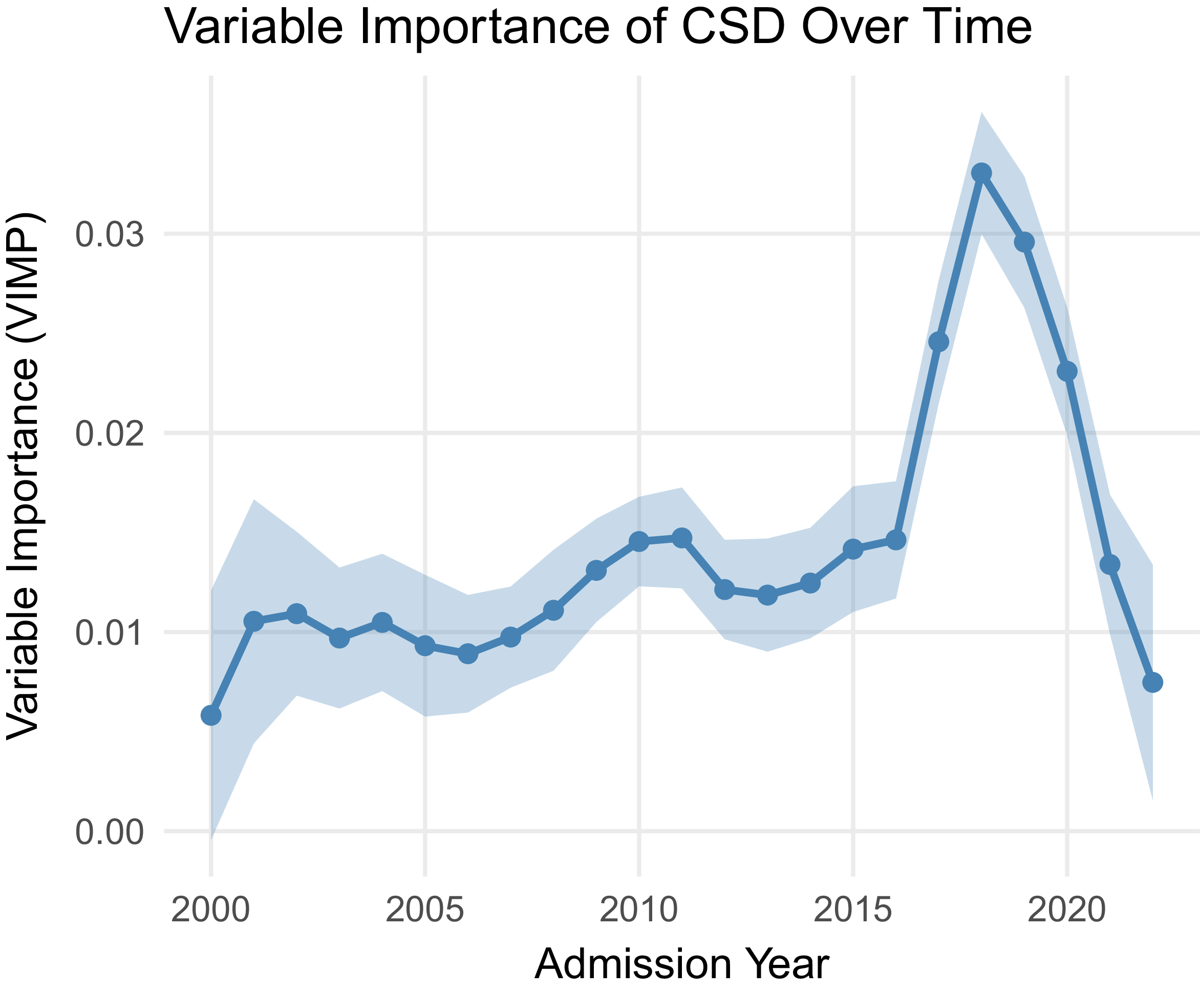
We next examine heterogeneity across admission cohorts. Figure 12 shows that the relative importance of the clinical and assessment variables changes materially over time. From 2000 to 2015, ADL is the dominant predictor in every admission cohort. Within this period, the overall ranking is fairly stable: CSD, BEH, and SEX typically form the next tier, while MBD, CHC, CMD, and MED are generally less influential. A clear shift emerges in the 2016–2020 cohorts. During these years, CSD becomes the leading predictor in most cohorts, and MBD also rises sharply into the upper tier. This suggests that depression-related symptoms and broader mental and behavioral diagnoses become substantially more informative in the more recent cohorts. The pattern changes again in 2021 and 2022. In 2021, ADL regains first place, while CSD and MED remain important. In 2022, ADL becomes overwhelmingly dominant and CHC rises to second place, whereas the importance of the mental and behavioral variables declines. Overall, Figure 12 indicates that the determinants of length of stay vary across admission cohorts, with the relative importance of physical dependency, depression, and diagnosis information shifting over time.
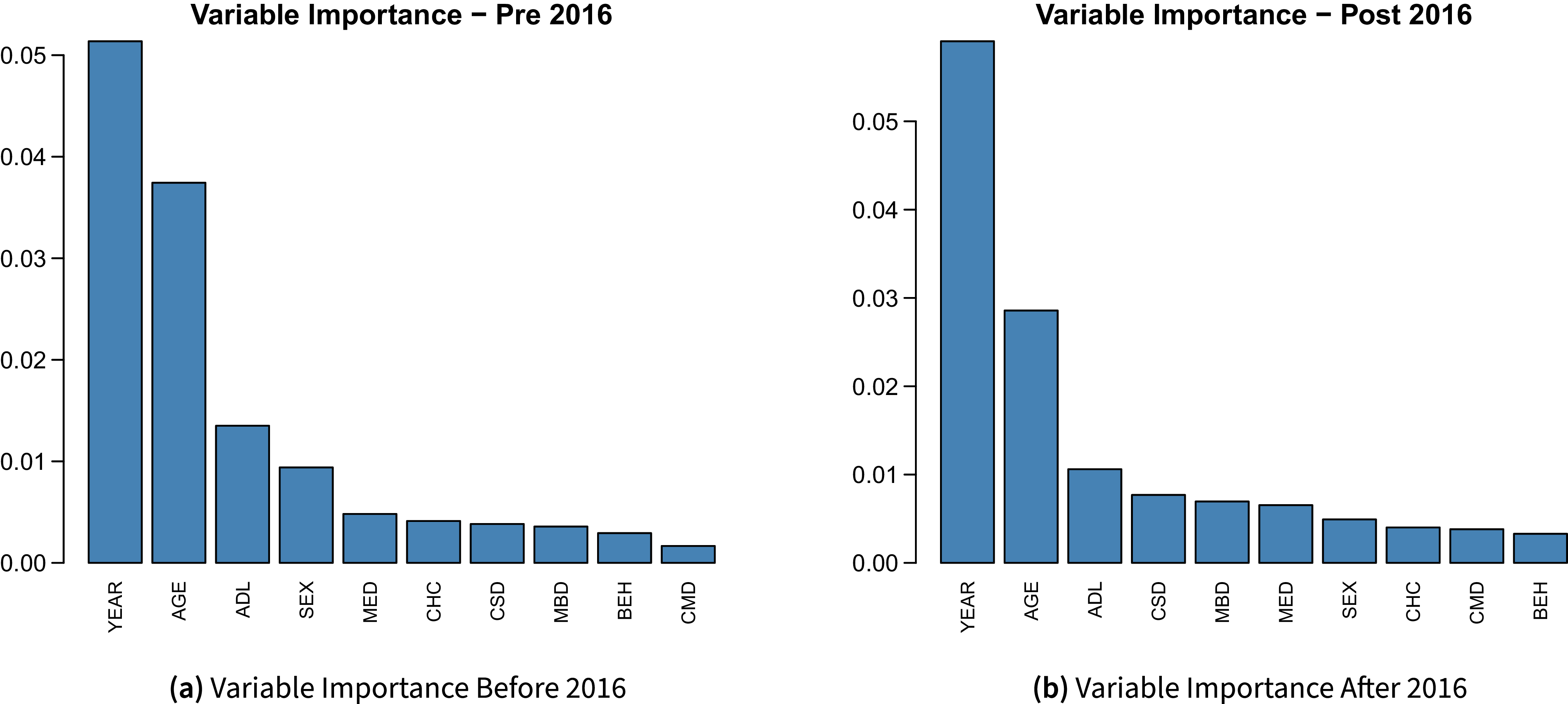
To investigate the observed shift in variable importance, particularly the rise of CSD in recent cohorts, we stratified the sample into pre-2016 and post-2016 periods, corresponding to the major ACFI reforms that took effect from 1 July 2016. These reforms primarily targeted the CHC domain, redesigning the scoring matrix and halving indexation of the CHC subsidy.
Shifts in variable importance before and after 2016.

Figure 13 reveals that CSD importance increases markedly in the post-2016 period. We interpret this as follows: the ACFI reforms systematically attenuated the signal carried by CHC-related variables. In the presence of a weakened CHC signal, the model naturally shifted predictive weight toward other informative variables, most notably CSD. Thus, the rise of CSD may be partially mediated by changes in the recording and funding of CHC needs, rather than reflecting solely a genuine change in the underlying resident population.
To assess the uncertainty of variable importance estimates for CSD, we employed the subsampling approach similar to Ishwaran and Kogalur (Reference Ishwaran and Kogalur2019). This method constructs standard errors and confidence intervals for permutation-based VIMP by repeatedly subsampling the original training data and re-computing VIMP on each subsample. Figure 14 shows the 95% confidence intervals along with the point estimates for CSD over admission years. As we can see, the confidence intervals for all the admission years do not contain 0, indicating the significance of importance of CSD.
Variable importance changes of CSD over time.

Heterogeneity across age groups is reported in Figure 15. In addition, we also constructed the bootstrapped confidence interval for ADL, CSD, CHC, and MED across different age groups, as demonstrated by Figure 16. The most prominent feature is the central role of ADL. It is the most important variable in all age groups except 50–54, where CHC is ranked slightly higher. At younger admission ages, especially from 50 to 64, CHC, MED, and CSD remain relatively prominent, indicating that CHC needs and broader medical burden are more informative in these groups. From age 65 onward, the ranking shifts. SEX moves into the upper tier and is the second most important variable for ages 65–89. At the same time, CSD becomes increasingly salient and ranks among the leading predictors from age 70 onward. By contrast, the importance of MED declines steadily with age and becomes negligible in the oldest groups. The two oldest groups also display a distinct pattern. For ages 90–94 and 95–99, CSD remains the second most important predictor after ADL, while CHC regains prominence in the 95–99 group. Taken together, Figure 15 suggests that the balance between physical dependency, depression, complex care needs, and broader medical burden varies systematically across the age distribution.
Changes in ranks of variable importance by age group.

Confidence intervals for VIMP of important variables across age group.

Overall, the subsample analysis leads to a clear conclusion: predictor importance is not constant across care-need profiles, admission cohorts, or age groups. Functional dependency remains fundamental throughout, but its role is systematically complemented by other variables. Broad medical diagnoses are more informative in lower-ADL strata and at younger old ages, whereas depression-related and mental-behavioral variables become especially important in higher-need groups and in more recent admission cohorts.
4.4 Discussion and implications
The results in this section convey a clear message. Although YEAR, AGE, and ADL remain the main predictors of length of stay, depression-related and mental-behavioral measures, especially CSD, provide important additional predictive power. Their role is most pronounced in higher-need ACFI strata and becomes more prominent in recent admission cohorts. Overall, the findings indicate that length of stay is shaped not only by demographics and physical dependency, but also by mood-related symptoms and diagnosis structure, particularly among residents with more complex care needs. More specifically, the subsample results show that broad medical diagnoses are relatively more informative in lower-need strata and at younger old ages, whereas depression-related and mental-behavioral variables become more prominent in higher-need groups and several recent admission cohorts. These cohort-specific shifts may also reflect major policy and assessment changes over time, with mental, behavioral, medical, and depression-related factors becoming more prominent in recent cohorts and potentially supporting more targeted resource allocation.
Our findings extend the Australian literature on residential aged care length of stay in several ways. First, in Zhang et al. (Reference Zhang, Shi and Huang2023), age, sex, marital status, and admission year are identified as key predictors using a weighted Cox framework. Our results further demonstrate that demographic factors alone do not capture the full heterogeneity in length of stay. Once detailed ACFI assessments and diagnosis information are incorporated, functional dependency remains central. However, depression-related and mental-behavioral variables also become important, particularly in higher-need strata. Relative to Zhang et al. (Reference Zhang, Shi and Huang2023), the present analysis therefore adds both richer resident-level information and a more flexible survival modeling framework.
Second, our results refine the conclusions of Fracalossi et al. (Reference Fracalossi, Zhang, Lee and Shi2025) on the importance of ACFI variables in two ways. First, their analysis models observed length of stay using conventional machine-learning methods on complete data only, rather than a survival framework that explicitly accounts for right-censoring for a richer and more informational sample. Second, their clinical information is mainly captured by dementia status and the three broad ACFI domains. By contrast, we introduce more detailed variables from Question 10 and the diagnosis sections, including CSD, CMD, MBD, and MED. Our results show that depression-related information is itself highly informative and, in several subsamples, more important than broader grouped measures. This refines the ACFI-based evidence in Fracalossi et al. (Reference Fracalossi, Zhang, Lee and Shi2025) by showing that mood disturbance deserves separate consideration.
Third, our study complements Xu and Yan (Reference Xu and Yan2025), which shows that facility and organizational characteristics also matter for length of stay in Australian residential aged care. While their focus is on institutional heterogeneity, our results emphasize resident-level clinical heterogeneity derived from the ACFI assessment framework. In particular, beyond demographic and institutional factors, detailed differences in dependency, mood disturbance, and diagnosis burden also play an important role in predicting length of stay for residential aged care.
Our findings have critical implications for actuarial and service-planning applications. Length of stay in residential aged care matters for expenditure forecasting, occupancy planning, and the valuation of accommodation-related liabilities (Xu & Yan, Reference Xu and Yan2025; Zhang et al., Reference Zhang, Shi and Huang2023). Our results therefore suggest that projections based only on demographic segmentation may miss important variation in duration risk. In particular, models of expected stay and case mix are likely to be more informative when they account for functional dependency together with depression-related and diagnosis variables.
These implications also place the analysis within the broader actuarial study of retirement and long-term care risk. Residential aged care LOS is a key determinant of the duration and uncertainty of care-related financial commitments, and therefore sits at the intersection of biometric modeling and financial planning. In this sense, the present analysis speaks directly to the interaction between insurance-type risks associated with health, frailty, and mortality, and the financial management of long-dated care obligations.
The findings also have a model-risk dimension. If LOS is modeled using frameworks that impose restrictive proportional hazards or linearity assumptions, important heterogeneity in care duration may be missed. A more flexible survival-learning approach can therefore be viewed as part of a robustness agenda in actuarial modeling, helping reduce misspecification risk when projecting long-term care duration and associated liabilities.
Our research also sheds light on improving long-term care financing and provider planning. For instance, for residents with high care needs, depression-related and mental-behavioral indicators are critical predictors. Hence, they can be leveraged for improving risk stratification, scenario analysis, and resource planning where data and regulation permit. More broadly, our results support a more person-centered view of residential aged care duration, in which expected stay reflects the joint role of physical dependency, mood disturbance, and diagnosis complexity rather than demographics alone.
5. Conclusion
This study investigates length of stay in Australian residential aged care using a comprehensive dataset derived from the ACFI. In contrast to existing Australian studies that focus mainly on demographic, broad ACFI, dementia, or institutional factors (Fracalossi et al., Reference Fracalossi, Zhang, Lee and Shi2025; Xu & Yan, Reference Xu and Yan2025; Zhang et al., Reference Zhang, Shi and Huang2023), our analysis incorporates richer resident-level assessment and diagnosis information, including depression-related appraisal variables from Question 10 and grouped diagnosis variables from Questions 13 and 14. To accommodate the right-censored nature of the outcome, together with non-proportional hazards, nonlinear covariate effects, and strong dependence among predictors, we employ the AORSF.
Our results show that admission year, age at admission, and functional dependency remain the main predictors of length of stay at the overall level. However, once richer variables derived from the ACFI are introduced, depression-related and mental and behavioral factors also emerge as important predictors. In particular, the CSD provides substantial predictive information beyond the broader ACFI domain measures, and its importance varies across residents. In the subsample analyses, the CSD and MBD become much more prominent in higher-need groups, especially when both ADL and CHC needs are high. The relative importance of the predictors also changes across admission cohorts and age groups, indicating that the determinants of length of stay are heterogeneous rather than stable across the residential aged care population.
These findings substantially complement the existing literature in several ways. Relative to Zhang et al. (Reference Zhang, Shi and Huang2023), our paper considers a richer set of care-need and diagnosis variables and adopts a more flexible survival-learning framework. Compared with Fracalossi et al. (Reference Fracalossi, Zhang, Lee and Shi2025), our analysis explicitly accounts for right-censoring and shows that depression-related variables deserve separate consideration rather than being absorbed into broader behavioral or dementia-related measures. With respect to Xu & Yan (Reference Xu and Yan2025), which emphasizes institutional and facility-level heterogeneity, our results highlight the importance of resident-level clinical heterogeneity.
Our study provides critical actuarial implications. Length of stay is closely related to expenditure forecasting, bed demand, care-mix planning, and the valuation of accommodation-related commitments in residential aged care. The present findings suggest that actuarial models of length of stay and long-term care commitments should move beyond demographic segmentation alone. In particular, projections of expected stay and resource use should account more explicitly for functional dependency, depression severity, and diagnosis structure. Ignoring these dimensions may understate the heterogeneity of duration risk across residents and reduce the precision of planning and funding decisions.
More broadly, the paper highlights how long-term care duration modeling contributes to the actuarial understanding of retirement-related risks by linking resident-level biometric heterogeneity to the financial assessment of long-dated care commitments. This connection between biometric risk and financial planning is central to contemporary work at the interface of insurance, pensions, and aged-care systems.
Future research could proceed in two directions. First, newer admission cohorts and linked datasets, such as those based on the Australian National Aged Care Classification funding model, could be incorporated into the analysis. Second, combining resident-level assessment variables with institutional characteristics, as examined by Xu & Yan (Reference Xu and Yan2025), may further improve forecasting accuracy.
Data availability statement
This study uses de-identified administrative records derived from the Australian Institute of Health and Welfare. The authors do not have permission to share the raw data.
Funding statement
This work received no specific grant from any funding agency, commercial, or not-for-profit sectors.
Competing interests
The authors declare no competing interests.





 Open access

