INTRODUCTION
What are abundance–occupancy relationships?
There are three possible types of relationships between the density of individuals of a species (that is the number per unit of space) and the size of the total area occupied by that species (that is the sum of all locations where it occurs). Firstly, the density of individuals within the occupied area can remain constant as the area occupied changes (Type 1 relationship in the Appendix). Secondly, the density of individuals may change as the area occupied changes in a consistent manner (Type 2 relationship in the Appendix). Thirdly, the density of individuals may change but the area occupied may remain constant (Type 3 relationship in the Appendix). Of these three possibilities, a positive relationship of the second type is by far the most common and is usually referred to as an abundance–occupancy relationship (Brown, Reference Brown1984; Gaston, Reference Gaston1996; Gaston et al., Reference Gaston, Blackburn, Greenwood, Gregory, Quinn and Lawton2000). In its general form, the ‘classic’ abundance–occupancy relationship states that as the number of locations where a species occur changes, the local density of individuals will also change in a similar direction (Brown, Reference Brown1984; Gaston, Reference Gaston1996; Gaston et al., Reference Gaston, Blackburn, Greenwood, Gregory, Quinn and Lawton2000). More specifically, it means that when a species occupies a large number of sites within an area, it will also have a higher average density of individuals across those sites where it occurs and vice versa. As a result, density will change at a faster rate than the number of sites occupied. However, why the density of individuals and the area occupied should generally be related in this manner, and not follow either of the other two possible relationships, remains unclear (Gaston et al., Reference Gaston, Blackburn and Lawton1997a).
Are abundance–occupancy relationships universal?
A positive relationship between abundance and occupancy is one of the most robust and widely documented patterns in macro-ecology (Gaston, Reference Gaston1996). Such relationships have been described in taxa as diverse as birds and terrestrial plants to fish and diatom assemblages (Crecco & Overholtz Reference Crecco and Overholtz1990; Swain & Wade Reference Swain and Wade1993; Gaston et al., Reference Gaston, Blackburn and Gregory1997b, Reference Gaston, Blackburn and Gregoryc; Blackburn et al., Reference Blackburn, Gaston, Greenwood and Gregory1998; Johnson, Reference Johnson1998; Falster et al., Reference Falster, Murray and Lepschi2001; Foggo et al., Reference Foggo, Frost and Attril2003; Fisher & Frank, Reference Fisher and Frank2004; Frost et al., Reference Frost, Atrill, Rowden and Foggo2004; Soininen & Heino Reference Soininen and Heino2005; Zuckerberg et al., Reference Zuckerberg, Porter and Corwin2009), for many different biogeographical regions (e.g. Gaston et al., Reference Gaston, Blackburn and Gregory1997b; Johnson, Reference Johnson1998; Fisher & Frank, Reference Fisher and Frank2004; Soininen & Heino Reference Soininen and Heino2005; Zuckerberg et al., Reference Zuckerberg, Porter and Corwin2009) and exists both within and across species (for a review see Gaston et al., Reference Gaston, Blackburn, Greenwood, Gregory, Quinn and Lawton2000). However, despite its widespread occurrence, there are some exceptions to this general ecological principle. For example, changes in abundance have been shown not to correlate with changes in occupancy in herbaceous flora (Thompson et al., Reference Thompson, Hodgson and Gaston1998) and in Australian passerines (Symonds & Johnson, Reference Symonds and Johnson2006). Furthermore, not all abundance–occupancy relationships take the same form, with Conrad et al. (Reference Conrad, Perry and Woiward2001) demonstrating a time lag between the decline in abundance of the arctiid moth, Arctia caja (Linnaeus), and the decline in its occupancy.
Do abundance–occupancy relationships exist in cetaceans?
Although a significant amount of research has been undertaken to document these fundamental ecological relationships in various taxonomic groups, there are few examples for marine systems and further research is required for varying combinations of scale, taxa and regions (Gaston, Reference Gaston1996). Therefore, while the main focus of research on abundance–occupancy relationships is now shifting towards identifying the mechanisms behind them, with varying levels of success, there are still many groups of organisms for which the existence of such patterns have yet to be documented. This includes cetaceans, in which there have been no previous studies of the relationship between abundance and occupancy. Thus, the aim of this study was to examine whether there is any evidence that abundance–occupancy relationships, both within and across species, exist in cetaceans.
MATERIALS AND METHODS
Data collection
Data were collected from 104 surveys along passenger ferry routes throughout the study area on the west coast of Scotland (Figure 1). At least four surveys were conducted per month throughout the study period, during May–July in 2003, 2004 and 2006 and June–August in 2005. These ferry routes can be considered as fixed transects, thus allowing the same area to be surveyed repeatedly in different months and years, providing spatial consistency in the survey effort between different time periods.
Study area on the west coast of Scotland. The black lines represent all survey effort in sea states of less than two for dolphins and porpoises. Grey lines represent the boundaries between the five regions: (a) Sea of Hebrides; (b) Straits of Tiree; (c) Inner Firth of Lorne; (d) Outer Firth of Lorne; and the narrow channel by the Isle of Mull is the Sound of Mull. Note: relative density and occupancy values were only calculated and analysed within the surveyed areas of each region and not for the whole extent of each region as defined by the boundaries in this figure.

The surveys were conducted by trained and experienced observers using two separate passenger ferries as research platforms. The ferries were virtually identical and were the MV ‘Clansman’ (eye height for surveying: 14.7 m) and the MV ‘Lord of the Isles’ (eye height for surveying: 14.2 m), with both following regular routes from Oban to the islands of Coll, Tiree, Colonsay and Barra (Figure 1). A single observer was situated on the port (left) side of the ship's bridge and recorded the ship's position (latitude and longitude), direction of travel (bearing in degrees) and speed (km/h) every 15 minutes, using a Global Positioning System (GPS) receiver, to provide information on survey coverage and effort. Environmental parameters, including sea state and visibility were also recorded every 15 minutes. Observational scans were conducted of an area directly ahead of the ship to approximately 135 degrees from the bow using reticulated binoculars (7 × 50 EWP) or the naked eye on a regular basis. When a group of cetaceans was sighted, the following parameters were recorded: the time; ship's position; direction of travel; the relative bearing to the sighting (from the ship's bow) using a compass rose, the number of reticules vertically from the cetacean to either land or horizon; the species; and the group size. For the purposes of this study, a sighting was defined as a group of animals seen in close spatial (within a few body lengths) and temporal (within a few seconds) proximity to each other, apparently involved in the same behaviour.
Data processing
This study aimed to measure and compare relative cetacean density and occupancy within the surveyed sections of the study area for the same time period. To maximize the number of comparisons available for analysis and account for potential variation in local cetacean occurrence due to habitat preferences, the study area was divided into five separate regions. The division into regions was based on coarse-scale oceanographic parameters, such as water depth, currents and tidal regimes which would be expected to affect cetacean occurrence and density. The five regions were the Sound of Mull, Straits of Tiree, Sea of Hebrides, inner Firth of Lorne and outer Firth of Lorne (Figure 1).
Cetacean density and occupancy were compared only for the specific area surveyed within each of the five regions at a particular point in time. Therefore, it was important that the probability of missing cetaceans was relatively consistent across all areas around the transect line that were considered to have been surveyed. For the majority of commonly utilized cetacean survey techniques, cetacean detectability decreases with increasing distance from the observer. Therefore, only data from a relatively narrow strip width around the survey transect, where the probability of detection would be highest, were analysed and used to calculate survey effort (in km2). In addition, only data collected in Beaufort sea states of two or less were analysed to account for the fact that the presence of smaller cetaceans is likely to be missed at higher sea states (Palka, Reference Palka1996). However, there is still some variability in cetacean detectability within sea states between zero and two, particularly at greater distances. To account for this, a narrower strip width around the survey transect was used at higher sea states. For small cetaceans (dolphins and porpoises) a strip width of 300 m was used for sea state zero, 250 m for sea state one and 200 m for sea state two. For minke whales (Balaenoptera acutorostrata Lacépède, 1804), which are more detectable at greater distances at all sea states due to their larger size, a strip width of 500 m was used for sea state zero, 400 m for sea state one and 300 m for sea state two. These strip widths are highly conservative estimates of the detectability distances for different cetacean species based on previous experience of using these passenger ferries as research platforms. Furthermore, if any detection bias was to occur within these extremely narrow strip widths then it would most likely cause an equal bias to all calculated variables throughout the entire study area. Only areas that fell within these narrow strip widths were considered to have been surveyed, and any sightings that fell outside the appropriate survey strip width were not used in any subsequent calculations.
For each cetacean species recorded, two density indices were calculated for the surveyed area of each region in each surveyed month of each year. These were the relative density of groups and the relative density of individuals. The relative density of groups was used as a density variable to explore the potential effect of social group structure (which may be influenced by social rather than purely ecological factors) on any abundance–occupancy relationships identified. The relative density of individuals was calculated by dividing the total number of individuals for each cetacean species in the surveyed area of a particular region and time period by the total area surveyed (km2) within that region and time period. The relative density of groups was calculated by dividing the total number of sightings for each cetacean species in the surveyed area of a particular region and time period by the total area surveyed (km2) within that region and time period. For both of these variables, relative densities, rather than absolute densities, were calculated as the correction factor g(0) (which accounts for animals missed on the transect line due a number of factors, such as being away from the surface on a dive), has not yet been estimated for the research platforms utilized in this study. However, it was assumed that there would be a reasonable correlation between relative and absolute density values. In all cases, the relative densities calculated refer only to the areas surveyed and no attempts were made to extrapolate these relative densities to any surrounding, non-surveyed parts of any region.
In most macro-ecological studies, occupancy is calculated as the number of grid squares in which a species occurs (e.g. Gaston et al., Reference Gaston, Blackburn and Gregory1997c). In this study, a similar approach was used, but occupancy measurements were corrected for the spatial coverage of the surveys to ensure the occupancy measure was calculated from the same surveyed areas as the density values. One potentially important issue when investigating abundance–occupancy relationships is the resolution of grid cells used to identify the proportion of area occupied by a species. In terms of this study, based on extensive modelling, it is known that the spatial distribution of cetaceans in this area is closely linked to the fine-scale distribution of ecogeographical variables (EGVs) at a 1 km2 resolution, with the likelihood of occurrence varying over relatively short spatial scales depending on the combinations of EGVs present (MacLeod et al., Reference MacLeod, Mandleberg, Schweder, Bannon and Pierce2008; Bannon, unpublished analysis). Therefore, this grid cell resolution was used to calculate occupancy within each region for each time period. To calculate occupancy, a grid was placed over the entire study area and only grid cells with more than 10% of their area included in the strip width were considered as having being surveyed. For each region and time period, occupancy was calculated by dividing the total number of grid cells containing at least one sighting of a particular species by the total number of grid cells surveyed at least once. Again, this occupancy value refers only to the surveyed areas within a region and was not extrapolated to any surrounding, non-surveyed parts of any region.
Statistical analysis
In most abundance–occupancy studies, the density of individuals at specific locations is measured and the average density across these locations relates to the proportion of locations sampled where the species was recorded as present (referred to as the ‘standard’ format in the Appendix). Any significant positive relationship between these two variables then represents a classic abundance–occupancy relationship. However, due to the type of survey effort available for this study and the highly mobile nature of cetaceans, it was not possible to calculate both variables in this format. Instead, occupancy for a whole region for a specific time period was compared to the overall density within this region for the same time period. In this format, an abundance–occupancy relationship is identified when there is a curvilinear relationship between the untransformed density and occupancy measures (see the Appendix for details). This is because this represents a situation where the density of individuals changes at a faster rate than occupancy, and therefore, the density of individuals within occupied areas is higher when occupancy is higher. In contrast, when there is no abundance–occupancy relationship, this will be represented by either a linear relationship or no relationship between the two untransformed variables (see the Appendix for details).
Once it had been established whether the relationship within the data set was consistent with the classic abundance–occupancy relationship (i.e. the relationship between the untransformed variables was curvilinear—see the Appendix), the variables were log-transformed to improve normality and allow a Gaussian distribution to be applied. Generalized additive modelling (GAM) was then used to define the shape of this abundance–occupancy relationship and investigate whether it differed between different species and measures of density. Relative density was used as the independent variable as it is more likely that population abundance and/or density determines the area occupied than vice versa (Holt & Gaston, Reference Holt and Gaston2003). Each data point in the GAM represents a relative density and occupancy measurement for one species in one region of one month of one year. Separate models were run using relative density of groups and relative density of individuals as independent variables. Models were run for each cetacean species separately and then for all cetacean species together, with species included in the latter model as a fixed factor in order to test whether the form of the abundance–occupancy relationships differed between the four cetacean species tested.
Spatial and/or temporal autocorrelation were not specifically taken into account in the modelling process by, for example, using a generalized additive mixed model. We were interested in whether, as relative density changed between relatively large spatial areas (regions) and/or relatively long periods of time (months and/or years), occupancy also changed in a consistent manner, regardless of whether changes in both are driven by the same underlying factor not included in the model. As a result, if we had removed such autocorrelation we would potentially have removed, or reduced, the actual relationship we wished to investigate. However, in order to assess whether the identified relationship could be an artefact of other potential spatial biases within the data (i.e. some regions may always have higher values than others due to differences in habitat between them) and/or temporal biases (i.e. some months and/or years may have consistently higher values due to temporal variations in conditions), where possible, the models were repeated with region, month and year included as covariates.
Generalized additive models were used in this study, rather than the linear models used in previous studies of abundance–occupancy relationships, as there is no theoretical reason that the relationship between abundance and occupancy must be linear. GAMs are particularly useful in this respect because they do not make any a priori assumptions as to the shape of the relationship (i.e. whether the best fit is linear, curvilinear, sigmoidal etc). All statistical analysis was performed using the statistical software package Brodgar version 2.5.1 (Highland Statistics Ltd).
Assessing whether cell resolution affects abundance–occupancy relationships in cetaceans
Since occupancy was measured using a grid structure, it is possible that the resolution of this grid could influence whether or not a positive abundance–occupancy relationship was identified in the data. In particular, while the choice of a 1 km2 cell resolution was based on a detailed understanding of what determines the spatial distribution of cetaceans within the study area (e.g. MacLeod et al., Reference MacLeod, Mandleberg, Schweder, Bannon and Pierce2008), it may be that these relationships will only exist using such fine-scale resolutions and not when larger cell sizes are used to calculate occupancy. Therefore, using the harbour porpoise (Phocoena phocoena Linnaeus, 1758) as a case study, the intraspecific analysis was repeated using three cell sizes (1 km2, 25 km2 and 100 km2). If cell resolution has an influence on the abundance–occupancy relationship, it would be expected that a clear pattern of presence and strength of the relationship would be obtained when models based on these different scales are compared. If no such pattern exists, then it would suggest that abundance–occupancy relationships exist in cetaceans independent of the resolution of the grid used to calculate occupancy.
RESULTS
Four cetacean species were recorded during this study: the harbour porpoise, the bottlenose dolphin (Tursiops truncatus Montagu, 1821), the short-beaked common dolphin (Delphinus delphis Linnaeus, 1758) and the northern minke whale. In the summer months of 2003 to 2006, 5585 km2 were considered surveyed for the three small cetacean species and 8509 km2 for minke whales. A total of 248 sightings consisting of 542 animals were recorded within the survey strips, which corresponded to 180 harbour porpoise sightings, 10 bottlenose dolphin sightings, 16 common dolphin sightings and 42 minke whale sightings in total.
From all the possible combinations of individual species, regions, months and years, zero values (i.e. points in time and/or space where an individual species was not recorded within the relevant survey strip) were removed from any subsequent statistical analysis. This ensured that these values were not responsible for any apparent abundance–occupancy relationship (i.e. by forming a cluster of points at the base of the trend and thereby inflating the significance of any potential relationship). When all the untransformed density and occupancy values were compared, the relationships identified were curvilinear, indicating, that given the format used to measure density and occupancy in this study, a ‘classic’ abundance–occupancy relationship existed within the data (i.e. a Type 2 relationship as defined in the Appendix). The exact form of the abundance–occupancy relationship was then tested for each cetacean species separately and then for all cetacean species together, using the log-transformed density and log-transformed occupancy measures.
Intraspecific relationships
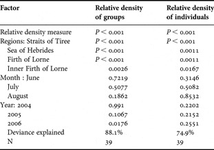
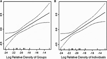
A positive, non-linear, relationship was identified between both log relative density of groups and log occupancy (Figure 2A, smoother P < 0.001, deviance explained = 45.3%, N = 39) and log relative density of individuals and log occupancy for harbour porpoise (Figure 2B, smoother P < 0.001, deviance explained = 46%, N = 39). When region, month and year were included in the relative density of groups GAM a significant abundance–occupancy relationship was still evident, with the model now explaining 88.1% of the deviance in occupancy. However, significant differences were noted for 2006 and for all regions, but not for month (Table 1). When region, month and year were included in the relative density of individuals GAM a significant non-linear relationship was still apparent, with the model now explaining 74.9% of the deviance in occupancy and significant differences noted for all regions, but not month and year (Table 1). Therefore, while there are some spatial and/or temporal biases within the harbour porpoise data, these biases are not sufficient to create a significant abundance–occupancy relationship where none exists. In addition, given the strength of the relationship between density and occupancy, it is extremely unlikely that it is an artefact of some underlying undetected bias.
Generalized additive model for harbour porpoise of: (A) log relative density of groups against log occupancy (P < 0.001, deviance explained= 45.3%, N= 39); (B) log relative density of individuals against log occupancy (P < 0.001, deviance explained= 46%, N= 39).

Results of the generalized additive model for both relative density of groups and relative density of individuals for harbour porpoise, with region, month and year as co-variates.

A positive, linear, relationship was identified for minke whales between both log relative density of groups and log occupancy (Figure 3A, smoother P < 0.05, deviance explained = 65.1%, N = 15) and log relative density of individuals and log occupancy (Figure 3B, smoother P < 0.05, deviance explained = 67.4%, N = 15). There were insufficient numbers of regions and time periods when minke whales were recorded (i.e. had non-zero values) to run a second GAM to assess the effect of other variables such as region, month and year on this relationship.
Generalized additive model for minke whale of: (A) log relative density of groups against log occupancy (P < 0.05, deviance explained= 65.1%, N= 15); (B) log relative density of individuals against log occupancy (P < 0.05, deviance explained= 67.4%, N= 15).

In contrast, no abundance–occupancy relationship was found for bottlenose dolphins using either log relative density of groups (smoother P > 0.05, deviance explained = 40.7%, N = 10) or log relative density of individuals (smoother P > 0.05, deviance explained = 48.6%, N = 10) as the density index. Similarly, there was no abundance–occupancy relationship for the common dolphin data, using either log relative density of groups (smoother P > 0.05, deviance explained = 1.0%, N = 10) or log relative density of individuals (smoother P > 0.05, deviance explained = 20.9%, N = 10).
Interspecific comparisons
When data from all four cetacean species were included in the same GAM, a significant, positive and non-linear relationship was found between log relative density of groups and log occupancy (Figure 4A, smoother P < 0.001, deviance explained = 64.3%, N = 74), with no significant differences between the four cetacean species noted. Therefore, all four species conform to the same relationships between occupancy and the density of groups within those sites occupied. In terms of the relative density of individuals, while there was still an overall significant, positive, non-linear relationship between log relative density of individuals and log occupancy, there were significant differences between the pairing of harbour porpoise and minke whales, and the other two species (Figure 4B, smoother P < 0.001, deviance explained = 57%, N = 74). This suggests that in terms of relative density of individuals, harbour porpoises and minke whales conform to the same abundance–occupancy relationship, but that common dolphin and bottlenose dolphin conform to significantly different abundance–occupancy relationships.
Scatterplot of the positive abundance–occupancy relationship for the four cetacean species recorded with the fitted smoother from the generalized additive model shown on the right for: (A) log relative density of groups against log occupancy (P < 0.001, deviance explained= 64.3%, N= 74); (B) log relative density of individuals against log occupancy (P < 0.001, deviance explained= 57%, N= 74). Different species are indicated by different shapes: diamond, harbour porpoise; square, bottlenose dolphin; triangle, minke whale; circle, common dolphin.

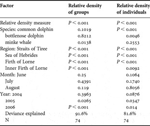
Furthermore, when potential spatial and/or temporal biases were accounted for in all the models, significant abundance–occupancy relationships were still apparent. For the relative density of groups GAM, using logged variables, a non-linear abundance–occupancy relationship was evident, with the model now explaining 91.6% of the deviance in occupancy and significant differences noted for minke whales, all regions, 2005 and 2006, but not month (Table 2). For the relative density of individuals GAM, using logged variables, a significant non-linear abundance–occupancy relationship was apparent, with the model explaining 81.6% of the deviance in occupancy and significant differences noted for common and bottlenose dolphins, all regions, 2005 and 2006, but not month (Table 2). Therefore, while there are some spatial and/or temporal biases within the dataset, these biases are not sufficient to create a significant abundance–occupancy relationship where none exists.
Results of the generalized additive model for both relative density of groups and relative density of individuals for all cetacean species, with region, month and year as co-variates.

The effect of cell resolution on the harbour porpoise abundance–occupancy relationship
Positive abundance–occupancy relationships were identified for harbour porpoise using both density indices at all cell resolutions tested. In both cases, the highest deviance explained was obtained using the 1 km2 cell resolution, followed by the 100 km2 cell resolution, whilst the lowest deviance explained was obtained using the 25 km2 cell resolution (Table 3). Therefore, a positive abundance–occupancy relationship exists at all spatial scales examined and the strength of this relationship does not decrease consistently with increasing cell size. As such, the identified relationships between abundance and occupancy at the 1 km2 cell resolution are unlikely to be an artefact of the cell resolution used to calculate occupancy.
Results of the generalized additive model for harbour porpoise at three different cell resolutions for both relative density of groups and relative density of individuals.

edf, estimated degrees of freedom.
DISCUSSION
Intraspecific relationships
Positive intraspecific abundance–occupancy relationships were found for both harbour porpoise and minke whales, using both density indices, within the surveyed areas of the west coast of Scotland. However, there was no relationship between abundance and occupancy in either common or bottlenose dolphins, using either density index. There is a possibility that this reflects the non-linear nature of the abundance–occupancy relationship in cetaceans, and that the relative densities at which these species were recorded fall within the portion of the overall non-linear relationship that has a slope at or close to zero at the lowest densities and occupancies (see Interspecific Comparisons). Alternatively, the sample size and/or the range of values for densities and occupancies recorded for these two species may have been too narrow to accurately estimate the true relationship between these variables. Further data are required, across a wider range of densities, in order to investigate whether either of these possibilities is correct.
Interspecific comparisons
In terms of the relative density of groups, all species examined conformed to the same abundance–occupancy relationship. The species composition at different points on this relationship varied from species with low density and low occupancy at the bottom left hand corner (common and bottlenose dolphins) towards species with high density and high occupancy (harbour porpoise and minke whales), with an overlap between these two groups at intermediate densities (Figure 4A). As a result, a consistent relationship was evident across all species even though not all intraspecific analyses demonstrated a relationship. Similar findings have been obtained for breeding birds, in which an overall interspecific relationship was evident (Gaston et al., Reference Gaston, Blackburn, Gregory and Greenwood1998), yet intraspecific analysis showed a variety of relationships to exist (Blackburn et al., Reference Blackburn, Gaston, Greenwood and Gregory1998).
In contrast, when the relative density of individuals was used as the density index, some species conformed to significantly different relationships. In particular, while minke whales and harbour porpoises conformed to the same abundance–occupancy relationship, the two dolphin species conformed to different abundance–occupancy relationships. This is most likely due to the differences in social structure between these pairs of species. While minke whales and harbour porpoises are predominantly solitary species (>60% of encounters were of single individuals), both bottlenose and common dolphins are more gregarious and commonly occur in groups (<50% of sightings were of single animals). This possibility is further supported by the fact that, within the study area, common dolphin occur in the largest and most variable group sizes and have the greatest difference, in terms of the coefficient of the model intercept, from the primarily solitary species whose sightings make up the majority of the data analysed (coefficients of common and bottlenose dolphins in comparison to harbour porpoise: –0.38 and –0.21). Therefore, for the interspecific relationship, occupancy is a more consistent measure of relative density of groups rather than relative density of individuals, due to potential differences in social structure between cetacean species.
Are the observed abundance–occupancy relationships an artefact of the survey and analysis methods used?
There are a number of potential factors within the design of this study that could have contributed towards the observed abundance–occupancy relationships in cetaceans. Firstly, the cell resolution used to identify the proportion of area occupied needs to be considered as a potential confounding factor. However, a positive abundance–occupancy relationship was identified for harbour porpoise at three different cell resolutions using both density indices. This relationship was stronger at the 1 km2 and 100 km2 resolutions compared to the 25 km2 resolution. This suggests that both the intraspecific and interspecific abundance–occupancy relationships identified in this study at the 1 km2 resolution are unlikely to be an artefact of the cell resolution used to calculate occupancy. It does, however, highlight that abundance–occupancy relationships identified at one spatial scale should not be directly applied to another spatial scale. The fact that the 1 km2 resolution performed the best in all of the models tested in this study is likely to be due to the influence of relatively fine-scale variations in habitat on the occurrence of cetaceans within this environmentally heterogeneous region (MacLeod et al., Reference MacLeod, Mandleberg, Schweder, Bannon and Pierce2008).
Secondly, the survey effort and analysis methods used need to be considered. There is no a priori reason that a given level of survey effort in different regions (or the same region at different times) will always give a correlated abundance and occupancy measurement unless there is an underlying relationship between these two variables. As a result, a positive abundance–occupancy relationship is unlikely to be generated by specific levels of survey coverage within a specific region. For example, for the same levels of effort and survey design, it is possible to identify any of the three possible forms of the relationship between the density of individuals and the occupancy within a region, given differences in how these two variables are related (see the Appendix). Therefore, the results of this study are unlikely to be an artefact of the methods used to collect, process, analyse or compare the data.
Thirdly, there is a possibility that the results are driven by spatial and/or temporal biases in the data. However, when such potential biases could be accounted for within the modelling process, while there were some differences between regions and years, there was still a significant relationship between occupancy and abundance for both relative density indices tested. Therefore, it is unlikely that the identified relationships are an artefact of such spatial and/or temporal biases. Finally, this study used a relative density of cetaceans as an index of abundance rather than measuring the absolute density directly. While it would be expected that variations in relative density would reflect variations in absolute density, this study was not able to empirically test whether these are directly comparable.
Despite these factors, this study demonstrates that cetaceans can be added to the great diversity of taxa for which this most general pattern in macro-ecology applies. However, differences in social structure between cetacean species need to be accounted for when comparing abundance–occupancy relationships between species, as while all species conform to the same relationship for the relative density of groups, species with different social structures differ in terms of the form of the relationship with the relative density of individuals. Nevertheless, the positive relationships identified here suggest that any change in the local density of a cetacean species is likely to be mirrored by a change in occupancy, with a species being recorded in more grid cells when its density per grid cell occupied is higher and fewer grid cells when its density per grid cell occupied is lower.
Implications of abundance–occupancy relationships for cetacean conservation and management
The existence of positive abundance–occupancy relationships in cetaceans has a number of important implications for cetacean conservation and management. Firstly, a positive abundance–occupancy relationship implies that species (or populations) that decline in range size can face ‘double jeopardy’ (Lawton, Reference Lawton1993), due to being simultaneously at risk from small geographical range size and low local abundance, hence facing a higher likelihood of extinction. As climate change is likely to result in a decline in range size for many species that are limited to cooler waters (Learmonth et al., Reference Learmonth, MacLeod, Santos, Pierce, Crick and Robinson2006; MacLeod, Reference MacLeod2009), a positive abundance–occupancy relationship implies that any such declines in range size may be accompanied by a corresponding decline in density and, therefore, overall abundance.
Secondly, the exclusion of a population from part of their range could result in a decline in population size, particularly if it is prolonged and there are no other neighbouring, but unoccupied, areas of suitable habitat for individuals to move into. This exclusion could arise due to various anthropogenic activities, for example, noise impacts associated with oil and gas activities and wind turbines (e.g. Carstensen et al., Reference Carstensen, Henriksen and Teilmann2006; Stone & Tasker, Reference Stone and Tasker2006; Thomsen et al., Reference Thomsen, Lüdemann, Kafemann and Piper2006), military activities (Parsons et al., Reference Parsons, Dolman, Wright, Rose and Burns2000), acoustic deterrent devices in relation to aquaculture (e.g. Johnston, Reference Johnston2002; Morton & Symonds, Reference Morton and Symonds2002; Olesiuk et al., Reference Olesiuk, Nichol, Sowden and Ford2002), as well increased boat traffic in relation to the development of marinas and whale-watching activities (e.g. Lusseau, Reference Lusseau2005).
Thirdly, a positive abundance–occupancy relationship is relevant for the establishment of marine protected areas (MPAs). In particular, if the aim of a specific MPA is to aid an increase in the size of a particular population, it will need to provide a sufficient area for that population to expand into. Consequently, buffer zones around proposed MPAs may be needed. Similarly, if only part of a species range is protected and the population is adversely affected outside this protected range, then the overall population may decline to the size that the MPA can support. Therefore, it is important to ensure the MPA is not too small in order for a viable and genetically diverse population to be supported. As such, the existence of a positive abundance–occupancy relationship for cetaceans may aid in identifying the minimum size required by an MPA in order to maintain such population sizes.
Finally, by examining changes in occupied grid cells over time, occupancy may be able to provide additional information on changes in abundance of a cetacean species within a specific area, as well as changes in species range and/or changes in spatial aggregations (e.g. MacLeod et al., Reference MacLeod, Brereton and Martin2009). All of this may provide further information on changes in population status for cetacean species, potentially aiding cetacean conservation and management strategies.
Although this study has demonstrated the existence of abundance–occupancy relationships in the cetacean community of the west coast of Scotland, before their full implications for cetacean conservation can be investigated, it is important to establish whether such relationships also exist in other cetacean species and in other geographical locations. Where possible this should be tested measuring absolute densities rather than relative densities to ensure that the relationships still hold under such conditions. Careful consideration of the differences in social structure between cetacean species will also be required, as well as ensuring that the cell resolution used to calculate occupancy is appropriate to the cetacean species and study area being tested.
ACKNOWLEDGEMENTS
The authors would like to thank the captains and crew of the Caledonian MacBrayne ferries (MV ‘Clansman’ and MV ‘Lord of the Isles’) for their help and assistance in making this project possible and also to all volunteers who helped collect data during the study. Funding was provided for K.H. through an MSc grant courtesy of NERC, C.D.M. and S.M.B. were funded through DSTL and G.J.P. was funded through the ANIMATE project (MEXC-CT-2006-042337).
Appendix
Examples of the three possible types of relationship between abundance and occupancy: Type 1: the density of animals within the occupied area remains the same as the occupied area changes; Type 2: the density of animals within the occupied areas changes as the occupied area changes; Type 3: the density of animals within the occupied area changes but the area occupied may remain constant. Of these three possibilities, only Type 2 relationships are considered ‘classic’ abundance–occupancy relationships, as in the other two cases the density of individuals within the occupied areas does not change as the area of occupancy changes. Theoretical examples are provided for each type of relationship assuming a study area of 100 km2 that has been divided into 1 km2 grid cells. The form of the relationships between abundance and occupancy are presented for each type based on these theoretical examples. These are provided in the ‘standard format’ (density of individuals within the occupied areas versus the size of the occupied areas) and in the ‘format’ used in this study (density of individuals within the whole study area versus the proportion of grid cells within the study area which are occupied). In the standard format, ‘classic’ abundance-occupancy relationships (Type 2) are represented by a significant relationship between the two variables indicating that as the size of the area occupied increases so does the density within those areas. In the format used in this study, ‘classic’ abundance–occupancy relationships (Type 2) are represented by a curvilinear relationship between the measures of density and occupancy (before any data transformations are conducted to improve normality or for other reasons), such that the measure of density changes at a greater rate than that for occupancy. This indicates that as the size of the area occupied increases, the density of individuals within these areas increases. Theoretical ‘survey effort’ within these study areas is represented by two randomly-positioned parallel 10 km transects with a swath width of 1 km. The number of animals and number of occupied cells expected from this level of survey effort for each example is also provided. This demonstrates that given a specific level of survey effort, a ‘classic’ abundance–occupancy relationship (Type 2) will only be obtained from such survey effort if this represents the true underlying situation. This applies regardless of the ‘format’ used to express these relationships.