1. Introduction
In the 1990s, trade policies pushed for regional integration in Latin America and the Caribbean. In the 2000s, a new modality emerged in which integration has been driven mainly by bilateral agreements both with other countries in the region and with countries in other regions of the world (ECLAC, 2006). Chilean leadership in this process has been clear. In the last 20 years, Chile has entered numerous Free Trade Agreements (FTAs) and in 2006, 74 per cent of total exports were under preferential agreements, the largest share in South America.
Chile has a small open economy that has based its economic growth on increasing exports,Footnote 1 mostly natural resources,Footnote 2 and responsible management of its main economic variables. Its stability over the last 20 years has improved Chile's international standing and attracted increasing levels of foreign direct investment (FDI).
For over two decades, Chile has engaged in a process of liberalizing its economy and has developed a trade policy based on three complementary strategies: (1) unilateral opening; (2) bilateral negotiations; and (3) multilateral negotiations, an approach similar to ‘open regionalism’. Unilateral opening has consisted of reducing tariffs from 15 per cent in 1990 to 6 per cent in 2006, for all products regardless of their origin or value. Only a few products were excluded under a price band system, such as wheat, sugar, oleaginous seed, and oil. After 1995, this strategy was subject to discussion and it was not clear whether reducing tariffs unilaterally should continue or if more emphasis should be put on FTAs with specific countries. Nor was it clear what the tradeoffs were associated with each strategy and whether complementary policies were required.
Even so, by 2006, Chile had signed trade agreements with most of its trade partners as part of a bilateral strategy oriented to increasing and securing market access. Initially, the negotiations focused on regional partners: Mexico 1990, Venezuela 1993, Colombia 1993, Ecuador 1994, Southern Cone Common Market (MERCOSUR) 1996, etc. Afterward, developed countries/areas were targeted: Canada and the USA 1997, the European Union, the European Free Trade Association and South Korea in 2002. In 2005, Chile focused on the Asian-Pacific Rim, finishing the P-4 Strategic Economic Partnership Agreement, the FTA with China and a framework agreement with India. Chile has signed an FTA with Peru, Japan, and China as well.
Despite this extensive level of international activity, there has been little empirical analysis of these agreements, and the work that has been done so far has usually operated within partial equilibrium frameworks. However, the impacts of an FTA negotiation spill over to the whole economy. General equilibrium analysis is necessary to identify the cause-effect chains and indirect effects that accumulate over time. Because of this, Computable General Equilibrium (CGE) models are increasingly being used to analyze such policies in other countries. For example, trade-related dynamic CGE models have been used to analyze the impacts of unilateral trade liberalizations (Zarazaga, Reference Zarazaga2000), migration in contexts of trade liberalization (Cogneau and Tapinos, Reference Cogneau and Tapinos1995), regional trade integrations (Diao et al., Reference Diao, Diaz-Bonilla and Robinson2002; Monteagudo and Watanuki, Reference Monteagudo and Watanuki2002; Roland-Holst and Van Der Mensbrugghe, Reference Roland-Holst and Van Der Mensbrugghe2002), trade reforms (Diao et al., Reference Diao, Yeldan and Roe1998), agriculture and trade (Storm, Reference Storm1997), external penalties (Canes, Reference Canes2000), environmental impacts of trade agreements (Gale, Reference Gale1994), FTAs and effects on employment (Gilbert, Reference Gilbert2003; Decreux et al., Reference Decreux, Guérin and Jean2003), and trade and environment linkages (Vennemo, Reference Vennemo1997). Dynamic impacts of trade liberalizations are extensively explored in trade literature (Srinivasan and Bhagwati, Reference Srinivasan, Bhagwati, Chipman and Kindleberger1980; Baldwin and Martin, Reference Baldwin and Martin1999). Several studies of the Uruguay and Doha Rounds have also incorporated variations on this mechanism. The use of the Global Trade Analysis Project (GTAP) database and model has allowed an extensive trade analysis. The development of the dynamic version of this worldwide CGE model facilitates long-term assessments.
Although most CGE applications use static models, interest in long-term forecasting and analysis of trends has triggered the flourishing of dynamic CGE models that explicitly incorporate the accumulation processes of an economy, thus increasing the mid-/long-term predictive capability of the simulations. Nevertheless, they increase the complexity of the assessment, adding the trends of economic variables to their interrelations in a specific period of time. Accumulation and distribution processes determine the final result. Therefore, there is a tradeoff between sectoral desegregation and dynamic specification (Pereira and Shoven, Reference Pereira and Shoven1988). Most dynamic CGEs are recursive and assume that agents are myopic; therefore, they do not incorporate the future in their current decisions. Each period is solved independently, although the evolution of capital stock links one period to another.
Some CGE models have also been applied to assess trade in Chile. Coeymans and Larraín (Reference Coeymans and Larraín1994) used a static model to study the consequences of joining the North American Free Trade Agreement (NAFTA). The model is set up for a small and open economy, and includes only six productive sectors and three regions that trade with each other (Chile, the United States, and the rest of the world). Data used for this study come mainly from the 1986 Input/Output (I/O) Table. The results showed that an agreement between Chile and the United States would generate a new pattern of trade composition with the United States and, in general, multiple benefits would follow. Harrison et al. (Reference Harrison, Rutherford and Tarr2003) used a multisector multicountry CGE model to compare different trade policy options. They concluded that due to preferential market access, additive regionalism is likely to provide Chile with many more benefits than the static welfare gains coming from the unilateral liberalization. Holland et al. (Reference Holland, Figueroa, Alvarez, Gilbert, Chumacero and Schmidt Hebbel2005) assessed imperfect labor mobility, urban employment and agricultural trade reform (considering price bands of selected commodities). The sustainable impact assessment of the trade aspects of the Association Agreement between the European Commission and Chile in 2002 included a GTAP-type CGE model as a first approach to identify the most affected sectors and the principal macroeconomic impacts. Rutherford and Tarr (Reference Rutherford and Tarr2003) developed a dynamic CGE based on their GTAP-type static version to assess the consequences of a Chilean FTA with MERCOSUR and NAFTA. The agreement with MERCOSUR resulted in reductions of welfare in Chile. The main finding is that there are equivalent effects on welfare in both the static and the dynamic versions of the model, although the dynamic model slightly underestimates the positive outcomes found in the static version. Cabezas (Reference Cabezas2003) reviewed most models on the FTA between Chile and the United States. Finally, Schuschny et al. (Reference Schuschny, Durán and de Miguel2008) analyzed Chile's trade policy with Japan and China, assessing the impacts on welfare and the economic structure of Chile. The document includes the changes in exports from environmentally sensitive industries.
The GTAP multicountry framework is adequate to assess feedbacks among trade partners. However, there is an important tradeoff with a more detailed assessment of intracountry impacts, in particular, fiscal and environmental ones. As an alternative, Beghin et al. (Reference Beghin, Bowland, Dessus, Roland-Holst and Van Der Mensbrugghe2002) used a more disaggregated model that considers 72 sectors and multiple trade partners, although it is not multicountry. Using their Trade and Environment Equilibrium Analysis (TEQUILA) model, they simulated the integration to NAFTA and MERCOSUR to quantify health impacts of the environmental consequences. However, it uses transferred coefficients to estimate the emissions of pollutants.
In this paper, we apply the Environmental Computable General Equilibrium Model (ECOGEM)-Chile model, an adapted version of the TEQUILA model, to examine the impacts and tradeoffs over time of the two trading schemes considered by ChileFootnote 3 in the 2000s, unilateral liberalization and trade-agreements with main partners. Three relevant policy issues are examined:
(1) The expected economic impacts of the trade policy, particularly on GDP and labor markets.
(2) The socioeconomic and environmental tradeoffs. The environmental consequences, usually not considered in these evaluations, are quantified both in terms of pressures on natural resource intensive sectors and local and global pollution. Emissions of pollutants are estimated based on coefficients developed specifically for Chile with domestic data. The social consequences, particularly distributive effects, are also addressed.
(3) Policy responses that may improve economic performance or mitigate negative outcomes of the trade policies. First, an increase of the value added tax (VAT) to compensate for the loss in fiscal revenues due to the reduction in external tariffs is analyzed. In 2003, the Chilean Government justified a one-point VAT increment, based on this type of consideration, but without any comprehensive analysis. Second, an external shock is considered, assuming an increase in FDI, particularly in natural resources-intensive sectors, based on an improvement of Chile's international reputation after the agreements.
Consequently, the main contribution of this paper is a better treatment of the agreements actually considered and finally implemented by Chile; the inclusion of a detailed analysis of policy responses to the expected reduction in government revenues due to the trade agreements;Footnote 4 a quantitative assessment of the pressures on the natural resource sectors affected; and an analysis of environmental consequences based on national data. These are key results that help focus policy responses when complex economic decisions – with multisectoral impacts – such as trade agreements are being considered.
In the following section, we present a concise description of the characteristics of the dynamic version of the ECOGEM-Chile model, the data used and assumptions of the initial trend or business-as-usual scenario. Section 3 discusses the macroeconomic impacts of the different trade policy scenarios. Section 4 presents the sectoral, environmental, and social impacts of business as usual (BAU) and the trade-policy scenarios. The following section presents the effects of two complementary scenarios to put into new context the trade agreements, a fiscal policy, and a foreign investment shock. Finally, Section 6 explains the main conclusions.
2. The dynamic ECOGEM-Chile model
The ECOGEM-Chile model has been designed to assess trade and environmental policies. It is a dynamic recursive CGE model.Footnote 5 It is divided into two components: (1) one static that is solved for selected points in time within the 1996–2020 forecast framework [these points are 1996 (base year), 1997, 2000, 2005, 2010, 2015, and 2020] and (2) the other dynamic that connects the static simulation periods through accumulation of productive capital, labor growth and, eventually, shifts in production technology.
2.1. The model
Most basic assumptions and characteristics of the static model, discussed in O'Ryan et al. (Reference O'Ryan, Miller and de Miguel2003) and O'Ryan et al. (Reference O'Ryan, de Miguel, Miller and Munasinghe2005) are also part of the dynamic version. It is a very detailed model that considers: disaggregation by productive sectors and services; labor and income groups’ differentiation; different consumption levels by socioeconomic groups; a variety of trading partners grouped in different trading blocks; and emissions of different pollutants, among others.
Sectoral production is modeled under constant returns to scale and cost optimization. Production technology is modeled as a constant elasticity of substitution (CES) nested function, with intermediate input substitution based on a Leontief function, and factors and energy following a nested CES. The supply of capital and labor factors is predetermined. The model includes factor-adjustment rigidities. In particular, two capital vintages (old and new) are considered, which drive substitution and rates of return. In addition, capital is assumed to be partially mobile. Labor is assumed to be mobile across sectors and, consistent with historical data, full employment is also assumed.Footnote 6
Consumption assumes an extended linear expenditure system function, which includes minimum subsistence consumption. Each representative consumer allocates optimally the disposable income among the different commodities and savings. The consumption/savings decision is completely static: savings is treated as a ‘good’ and its level is determined simultaneously with the demand for the other commodities, the price of saving being set arbitrarily as equal to the average price of consumer goods.
Imports are modeled with the Armington assumption, i.e., domestic and imported products are imperfect substitutes, whereas exports are modeled as a constant elasticity of transformation function, with domestic production as an imperfect substitute for exports. For both cases, imperfect substitution is also assumed for products from/to different regions of the world. Other final demands, government expenditure, investment expenditure, and transfers are assumed as fixed shares.
There are different types of taxes, subsidies, and transfers used by Chile's fiscal system. The government collects direct taxes, including labor taxes and household and business income taxes, import tariffs, VATs, and some specific taxation. As a closure condition for public finances, it is assumed that government savings is defined as flexible, while spending is fixed and equal to the original level previous to any simulation. Tax and transfer coefficients are kept constant.
In each period, the value of the demand for gross investment must equal the economy's net aggregate savings (equal to the sum of savings by firms, households, government, and net flows from abroad). This closure rule implies that investment is driven by savings. As well, the investment in each firm is distributed by relative rates of return. The last closure rule refers to balance of payment equilibrium, while the model numeraire is the nominal exchange rate.
The dynamic in the model is of the recursive type, in which agents are considered myopic and base their decisions on static expectations about prices and quantities. The dynamic structure of the model includes a semiputty capital substitution possibility. New capital (putty) has a higher degree of substitution than old capital (semiputty). Short-term or long-term elasticities can be chosen for the substitution between the factor nest and nonenergy-producing inputs, as well as for the CES between capital–energy and labor, between capital and energy, and for the various energy producing sectors.
To link one period to another, a behavioral equation for investment is included: savings (Investment) in period T is allocated as new capital in period T + 1. Investment is allocated across sectors until the relative rate of return is equalized among them, unless a given sector is reducing its output. In that particular case, the sector may disinvest part of its capital depending on the disinvestment elasticity. Inventory stocks are assumed to be reduced by 50 per cent each period. Other relevant variables in the dynamic model are GDP growth rate, population growth rate, and labor productivity growth rate. These variables are exogenous in the base case scenario and endogenously determined for the subsequent simulations, with the exception of population growth, which is always exogenous. Growth in the model is assumed to be of a Hicks-type since labor productivity and GDP growth determines capital productivity endogenously.
2.2. Air pollution in the model
The model has environmental features that allow for forecasting emissions of both local pollutants such as particulate material of 10 μm or less (PM-10) and a global pollutant, carbon dioxide (CO2). An important contribution of the paper is that the coefficients for these pollutants are obtained from econometric research based on Chilean data and adapted to the model. It also incorporates energy-input substitution as a mechanism to reduce emissions, since emissions are related to the use of different inputs, as well as to production and consumption levels. The ECOGEM-Chile model calculates total emissions following the approach of input use, via emission factors for production and consumption, although the production process may also emit per se according to empirical evidence. The following equation shows the application of these factors to calculate emissions in the model:

where EP is the amount of emissions of pollutant p – measured in physical units – which are released into the environment in 1 year; XPj is the value of the production by industry j; XApij is the value of a good i consumed as an input in industry j; XAhih is the value of the good i consumed by household type h; and XAfdif is the value of the good i consumed by another final demand component f. These values, measured in monetary units, are given by the social accounting matrix (SAM). Finally, emission factors by production and input-consumption are vPj and πPi, respectively, measured in tons emitted per monetary unit of the SAM.
As explained, the first term in equation (1) captures emissions generated in the production process of each sector that cannot be explained by input use. In this case, it is assumed that neither the working capital nor labor produces emissions. The second term is associated with the consumption of goods by firms and other actors considered in the model (these goods are, e.g., coal, oil and gas, and refined fuels).
The emission factors previously implemented in the ECOGEM-Chile model were adapted from Dessus et al. (Reference Dessus, Roland-Holst and Van Der Mensbrugghe1994), based on the industrial pollution projection system data, from the United States. This paper makes an innovation by using national emission factors, whose estimations followed the methodology of Dessus et al., but with data from Chile (Carriquiry, Reference Carriquiry2008). Thus, the national emission factors use data from the Registry of Emissions and Pollutant Transfer in Chile, which was implemented in the late 2007. Contaminants from this database include CO2 and PM-10. The major polluting activities in Chile are in the energy, manufacturing, and transport sectors. These three sectors account for 91 per cent of CO2 emissions and 72 per cent of PM-10 emissions.
2.3. The data and basic assumptions of the model
Since the simulation is for trade agreements signed in 2002 and 2003, we developed a 2001 SAM for the Chilean economy (O'Ryan et al., Reference O'Ryan, de Miguel, Miller and Lagos2002), based on the official 1996 input-matrix (Central Bank of Chile, 2003). It has 73 sectors; however, to follow the interrelations among variables and the adjustment process during the shocks in the dynamic framework, these were aggregated to 25 sectors. Particular emphasis is placed on the natural resource sectors. Skilled and unskilled labor, five types of consumption based on income-households, and five relevant trading groups of countries (USA, European Union, Rest of America, Japan and Rest of World) are also specifications of the SAM.
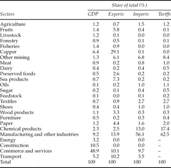
As a result of the variety of trade agreements signed by Chile, the share of tariffs among total revenues of the government declined. For the base year, tariffs were 12 per cent of government revenue, in comparison to specific taxes (11 per cent), VATs (47 per cent), and income taxes (24 per cent). Chilean exports are mainly from primary products, in particular natural resources-based sectors such as copper (table 1). On the other hand, imports include products with a higher degree of manufacturing. Manufactured goods, chemicals, along with other mining and textile products, provide most of the revenues from tariffs.
Sectors considered and structure of Chile's economy

Source: Authors, based on the Chilean I/O matrix.
Households have different consumption and savings characteristics depending on the income quintile they belong to. There is a high degree of inequality in Chile; therefore, the richest quintile receives 14 times as much income as the poorest.Footnote 7 Nevertheless, the poorest quintile receives almost 40 per cent of total income from government transfers, while the remaining 60 per cent comes from labor earnings.
Consumption patterns differ among income quintiles. In fact, the richest spend a larger proportion of their income on services (41 per cent for the fifth quintile vs. 31 per cent for the first quintile) and industrial products (36 per cent vs. 34 per cent), while the poorest quintiles spend a larger proportion on food (14 per cent for the fifth quintile vs. 23 per cent for the first quintile), and energy (2 per cent vs. 4 per cent).
The BAU scenario simulates the growth of the Chilean economy until 2020. Several assumptions must be made about the following variables: growth of GDP, labor force, population and labor productivity; as well as the share of foreign savings over GDP. For the baseline, the values used from 1996 to 2005 are the existing values for the Chilean economy. For the period 2006–2020, estimations of the growth of key variables prevalent in the period when the agreements were being considered are used. The trend assumes GDP annual growth rates of 5 per cent until 2010 and 4.5 per cent for 2010–2020.Footnote 8 Population, labor force, and labor productivity growth rates are assumed to be 1 per cent, 1.2 per cent, and 0.5 per cent, respectively, over the period 2006–2020. Finally, net foreign savings as a share of GDP are assumed to be 4.2 per cent for 1997 and are held constant at 1.5 per cent of GDP from 2000 on.Footnote 9
3. Macroeconomic effects of FTAs
Using the dynamic CGE model, in this section we analyze the macroeconomic effects of the two trade scenarios considered for Chile and compare them to BAU. Specifically, we focus on the impacts on GDP and wages. The first scenario consists of unilateral trade liberalization (UL) by Chile. In 2006, Chile's common external tariff was 6 per cent. For this reason, it is assumed that the policy consists of a unilateral six-point reduction in all tariffs for all countries.Footnote 10
The second scenario simulates the combined effects of trade agreements with the EU and USA (FTA EU-USA). A detailed analysis was carried out, sector by sector, defining specific reductions in tariffs to Chilean exports by the United States and EU. Tariffs from 14 productive sectors in the United States are considered, including important sectors such as textiles, shoes, and dairy products. For the European Union, 15 sectors are analyzed where livestock, preserved foods, shoes, and sea products stand out.Footnote 11 In the case of Chile, it was assumed that tariffs on imports from these countries are reduced by six points.
3.1. Impacts on GDP and wages
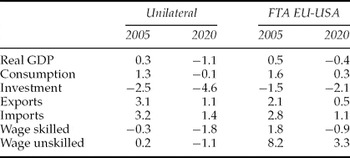
Trade liberalization improves growth – relative to BAU – in the short run, although this positive effect tends to revert in the long term. Trade agreements report better results than unilateral liberalization. Table 2 presents the expected impact on GDP and wages of skilled and unskilled workers between 2005 and 2020. The results correspond to the difference of each scenario with respect to the BAU path considered.
Macroeconomic results for Chile (percentage variation compared to the baseline)

Source: Authors, based on the ECOGEM-Chile model.
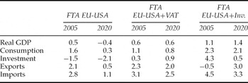
The GDP performs worse in the medium and long term under both scenarios compared to BAU. National product under FTA EU-USA increases less than under BAU from 2015 onward. Under UL, GDP only performs better up to 2005. Table 2 presents additional macroeconomic impacts for the short (2005) and long term (2020) that help to explain these results. Positive trade effects are compensated in the long run by a reduction in public domestic savings connected to the loss in tariff revenues. As this loss is not compensated by the rise in other revenues or by private savings, it causes a decrease in investment. Furthermore, as net exports decrease over time, the overall balance of Chilean GDP becomes negative.
As can be seen, a second surprising result that emerges from table 2 is that the effect on trade is rather weak, particularly in the combined FTA EU-USA scenario. Exports that put pressure on resources for their production would increase only modestly in the long run, compared to their growth in the BAU scenario.
The chain of events begins with the tariff reductions that generate a decrease in the price of imports. As expected, this leads to an increase in the demand for these products from both trading partners. Two effects appear. First, as imported inputs become cheaper, some sectors benefit from lower costs, increasing their competitiveness and consequently their output for domestic and foreign consumption. On the other hand, some sectors become less competitive since cheaper imports will replace domestic production to some extent. The first effect dominates in the short run, both in production and in exports. However, in the long run, the second effect is greater and dominates the GDP results and leads to a lower increase in exports. Therefore, the impact on production and exports depends on the timeframe being considered. There is an initial increase in aggregate exports that diminishes over time due to the equalization of domestic and import prices. Additionally, the effect on current accounts is initially small, but positive. However, the loss of competitiveness of domestic producers generates an increasing negative effect in the long run.
The main explanation for the reversal in the long run is that the tariff cut would reduce fiscal income compared to the base-line scenario. In particular, the reduction of tariff-related revenues under the UL scenario reaches 43 per cent in 2005, compared to only 24 per cent in the case of combined FTA EU-USA. This leads to a reduction in public savings,Footnote 12 which negatively affects total investment (−2.5 per cent to −4.6 per cent for unilateral liberalization and −1.5 to −2.1 for the FTA EU-USA). There are moderate increases in other revenues, but they do not compensate the shortfall of revenue from the tariff cutback. This affects some specific and sizeable sectors of the economy, such as construction, which decreases by a similar proportion to that of investment as compared to the baseline.
In summary, average growth rates over the period and the final GDP level will be slightly lower than in the base scenario for two main reasons: the loss of competitiveness of domestic sectors due to lower prices of imported goods, and the negative impact on investment of an uncompensated loss of fiscal revenue due to lower tariffs.
Wages increase under all scenarios as a result of the assumption that the economy grows in the baseline. However, table 2 shows that under both liberalization scenarios wages follow different and interesting paths that would have social impacts. These are analyzed in the next section. Skilled workers see a decline in their wages relative to BAU, except initially under FTA EU-USA where they increase by less than 2 per cent. This negative effect is more pronounced under unilateral liberalization. Unskilled workers benefit significantly under FTA EU-USA, however under UL, the impact is ambiguous: initial improvement is followed by a decrease in wages.
These results are explained by the major expansion of sectors that are intensive in the use of unskilled labor. In fact, as will be discussed in section 4, under the FTA EU-USA, fruits, agriculture, sea products, and preserved foods, which are sectors that basically employ unskilled labor, grow the most. Under UL, the main economic sectors grow less than under FTA EU-USA. Even though the copper sector, which employs relatively more skilled labor, increases compared to under BAU,Footnote 13 the increase is not sufficient to compensate for the decrease in the demand from other skilled-labor-intensive sectors, such as manufacturing, commerce, and services.
In conclusion, GDP under trade agreements with the EU and the United States performs better than under unilateral liberalization. Similarly, wages also perform better and unskilled workers see an absolute increase in their wages compared to under BAU. Establishing trade agreements with both trading partners is then clearly a dominant strategy considering these indicators.
4. Sectoral, environmental, and distributive impacts
Different trade liberalization policies have different impacts on natural resource-based sectors, local and global emissions, and social variables. These are analyzed below.
4.1. Impacts on natural resource-based sectors
Output of all natural resource-based sectors increases under any of the scenarios between 2005 and 2020, reflecting Chile's comparative advantage in these sectors. In the BAU scenario, copper production increases by almost three times in the period, agriculture and livestock by almost two times. Clearly, Chile's growth strategy will put significant pressure on water and land to develop these sectors as well as generate increasing environmental liabilities. Forestry and fisheries will also increase their production significantly.
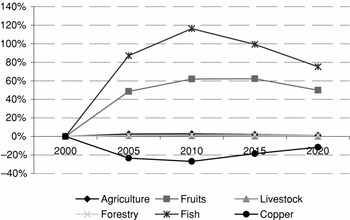
However, each type of agreement results in different impacts on natural resource-based sectors due to the changes in their relative profitability. The following figures present the differences in the paths of natural resource-based sectoral production compared to the BAU, due to the unilateral tariff reduction and the simultaneous FTA EU-USA.Footnote 14 The latter has a very significant impact on the fishery (around 100 per cent from 2010 on) and fruit sectors (60 per cent).
The important increase in the value of production of the fishery sector may be excessive and biologically unsustainable. It is however interesting to note that these exports to Europe effectively increased by 88 per cent, and to the United States by 33 per cent, between 2004 and 2008. Considering separately open fisheries and aquiculture – mainly salmon – the value of production of the former increased 46 per cent and of the latter by 60 per cent in the period. Consequently, the results of the model concur with observed data. However, this may not be sustainable in the longer term, at least for open fisheries, because of biological thresholds.Footnote 15 However, these results highlight the stress to which these sectors may be exposed due to liberalization. Unilateral liberalization has a much lower impact, lower than 6 per cent on the value of production of the affected sectors.
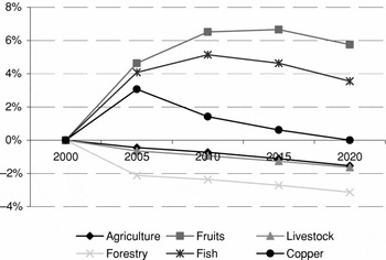
Under unilateral liberalization, the natural resource sectors that improve their production relative to BAU are fruits, fish, and copper. Forestry, livestock, and agriculture are negatively affected (figure 1). On the other hand, simultaneous FTA EU-USA also significantly benefits fisheries and fruits, and additionally, agriculture, forestry and livestock. However, production in the copper sector grows less than under BAU (figure 2).
Path of impacts on sectoral production with unilateral liberalization (percentage variation compared to the baseline)

Path of impacts on sectoral production with simultaneous FTA EU-USA (percentage variation compared to the baseline)

Sectoral results are explained by changes in relative profitability. Increasing production in a specific sector requires new investment. However, in these scenarios, there are no additional sources of financing associated with the agreements. Consequently, since overall savings decrease, the adjustment has to be made among sectors and factors. Therefore, the sectors with comparative advantages after the agreement will demand resources (mainly capital and labor) from those less favored.
The specific sectors affected depend ultimately on the characteristics of each agreement. For example, copper production is lower under FTA EU-USA compared to BAU, while the contrary occurs under UL. Under FTA EU-USA, noncopper exporting sectors are favored strongly by the reduced tariffs. As a result, exports of fruits, preserved foods, and sea products increase relatively. This generates an increase in the terms of trade and in the demand for capital and labor, increasing the price of each, which is not compensated by the reduction in tariffs, resulting in a reduction in the production of the copper. Under UL, even though exports in the aforementioned sectors also increase relative to BAU, the magnitude of the increase is much lower. The pressure on relevant prices for copper is much less, and its production finally increases more than under BAU as a result of the reduction in tariffs.
4.2. Environmental impacts
The simulation based on Chilean coefficients shows that absolute levels of CO2 and PM-10 emissions increase significantly under BAU between 2005 and 2020, reflecting the weight in environmentally sensitive industries in Chile: CO2 increases by 90 per cent and PM-10 by 80 per cent. This obviously would put a burden on regulators, both to control local pollutants and to comply with future restrictions on greenhouse gas emissions.Footnote 16
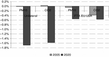
Trade liberalization does not change this situation dramatically. Figure 3 suggests that both PM-10 and CO2 emissions decrease – relative to BAU – but not significantly. The maximum reduction – around 1.6 per cent in 2020 – happens with unilateral liberalization, which presents higher reductions than FTA EU-USA in the long run, whereas FTA EU-USA reduces emissions more in the initial period. This is because under UL, the sectoral productions that fall more in the long run are manufacturing and energy (which represent 80 per cent and 70 per cent of CO2 and PM-10, respectively). On the other hand, with FTA EU-USA, these two sectors are less affected; therefore, their emissions experience less variation; while the copper sector, the sixth largest CO2 emitter, grows less than it would in the case of UL, and as a result the reduction in emissions is relatively higher in the short term.
Environmental effects (percentage variation compared to the baseline)

4.3. Social impacts
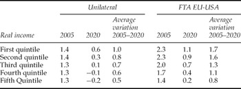
Table 3 shows that both trade policies improve income for all quintiles (with the exception of the richest in the case of UL in the long run). Lower domestic prices, combined with an increase in wages, especially those of unskilled labor, have a positive effect over real disposable income for all households.
Real disposable income by quintile (percentage variation compared to the baseline)

Source: Authors, based on the ECOGEM-Chile model.
This effect is higher for the poorer quintile groups. Indeed, for the FTA EU-USA scenario, the poorest quintile increases income – in the period – by 1.7 per cent compared to 0.8 per cent for the richest. For the UL, this effect is also progressive but lower than the FTA EU-USA (table 3). This is explained by the fact that the winning sectors are unskilled labor intensive.
In conclusion, there are tradeoffs associated with each agreement compared to BAU. The fruit and fishery sectors will receive increased demands under both trade agreements, forcing overexploitation of biomass stocks and affecting quality and availability of productive land. However, these effects will be much stronger under the FTA EU-USA. On the other hand, in relation to BAU, both trade agreements will improve air quality and contribute less to climate change. However, under the FTA EU-USA, emissions are lower in the short run, while UL performs better in the long run. Finally, income distribution improves under both agreements, though this effect is much stronger under the FTA EU-USA.
5. Additional investment and VAT policies
During the discussions in Chile, policy makers argued that FTAs with the EU and the United States would also offer additional positive effects that would increase FDI. The argument was mainly that an FTA would attract foreign investors since the country would be perceived as a safer place to undertake business. For example, through lower country risk premiums and/or policies to promote investments, such as parallel international double taxation agreements or accelerated capital depreciation rules.Footnote 17 Policy makers who were also concerned with the reduction in revenue from lower tariffs proposed an increase in VAT to offset the reduction in fiscal revenues due to the agreements.
In this section, we simulate both of these cases. The first scenario considers the FTAs with an increase in foreign investments, and the second one the FTAs with an increase in the VAT to keep fiscal revenues constant.
In the FDI scenario, we double foreign savings for the period 2005–2010, assuming it is a positive supplementary effect from the FTA EU-USA.Footnote 18 Additional savings trigger an increase in investment in the more competitive sectors, improving economic performance. Thus investment capital is not constrained and competitive exporting sectors develop without draining resources from the rest.
The second scenario – trade agreements together with an increase in VAT to keep public ‘savings’ constant – is similar to the policies applied by the Chilean government: (1) FTA with USA (2003), (2) FTA with EU (2002), (3) increase in VAT by one point, reaching 19 per centFootnote 19 to mitigate the negative effect on the public budget of decreasing tariff revenues.
5.2. Macroeconomic effects
As a result of both complementary policies, macroeconomic performance improves significantly (table 4), particularly in the long run. There is a significant increase in GDP – between 1 per cent and 2 per cent over the period – compared to the baseline. Absorption overreacts in the short run (2.5 per cent–3.2 per cent), prompting a strong increase of imports (trade + investment effect), which moderates over time. The initial impact of the agreements, plus higher external savings, also hits current accounts initially, but this effect is reversed by the end of the period, when investment in winning exporting sectors takes place. Consumption also increases compared to prior simulations.
Macroeconomic results for FTA EU-USA plus VAT and investment (%) (percentage variation compared to the baseline)

Source: Authors, based on the ECOGEM-Chile model.
The results also show that to keep public savings constant, it would be necessary to increase VAT by 1.35 points to 19.35 per cent. This is an interesting result, which is slightly higher than the 1 per cent increase that was actually implemented in 2003.
5.3. Distributive effects
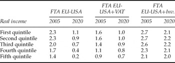
Table 5 presents the main distributive impacts under the new scenarios. A first conclusion is that all quintiles improve their incomes under the FTA EU-USA scenario with the VAT and investment scenarios.
Distributive effects for FTA EU-USA plus VAT and investment (percentage variation compared to the baseline)

Source: Authors, based on the ECOGEM-Chile model.
In addition, it can be concluded that all but one scenario are progressive, i.e., the poorest groups benefit more than the richest, compared to BAU. Under the higher foreign investment scenario, impacts on income distribution seem more neutral and the middle-income groups benefit the most, offsetting the progressive effect obtained from the FTA EU-USA. Nevertheless, it has the most positive impact on income level for all households. In the VAT scenario, since the poorest sector consumes a larger share of its income, an increase in this tax reduces the progressivity of the trade policy.
The complementary scenarios present differences between the long and short run. In the short run, both are progressive, but slightly less than in the FTA EU-USA scenario. The long run is less progressive than the short run, especially under the investment scenario.
5.4. Impact on emissions
Impacts on emissions depend on the specific scenarios since they are directly related to the winning and losing sectors and their relative sizes in the economy. In fact, changes in emissions are the result of a scale effect that increases emissions in each sector as it grows and a composition effect that can increase or reduce emissions, depending on the emission intensity of the sectors that grow or shrink relative to BAU.
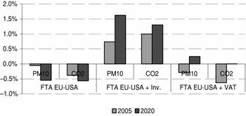
As can be seen in figure 4, the scale effect dominates in the investment scenario and consequently emissions of both PM-10 and CO2 increase relative to BAU.Footnote 20 Under the VAT scenario, growth is not as strong and the composition effect dominates in the short run, allowing a reduction in emissions relative to the BAU. In the long run, emissions increase slightly.
FTA EU-USA plus VAT and investment: environmental effects (percentage variation compared to the baseline)

The differences in CO2 emissions are summarized in the performance of the manufacturing, transport, energy, copper, and sea products sectors. The FTAs, independent of the scenario, generate a reduction in copper emissions and an increase in transport and sea products emissions. The behaviors of the energy and manufacturing sectors depend on the scenario. For example, in the FTA EU-USA and VAT scenarios, CO2 energy emissions always decrease. By contrast, energy emissions in the FDI scenario increase strongly throughout the period.
The PM-10 emissions are driven mostly by the same sectors. Independent of the scenario, emissions from copper production always decrease, while those from fisheries and sea products rise. The contribution to emissions from manufacturing is only relevant in the FDI scenario, while energy emissions increase progressively over time. Alternatively, in the FTA EU-USA and VAT scenario, energy emissions show a decrease throughout the period.
In terms of climate change, although developing countries do not have absolute CO2 reduction targets, middle-income countries like Chile will have to contribute to mitigating this global challenge. Their contributions are usually in terms of reducing CO2/GDP intensity, which is also the path that Chile is following. Results show that an FTA allows for lower emission intensities by around 8 per cent over the period in the best-efficiency scenario (FTA EU-USA increasing VAT).Footnote 21 This is an interesting conclusion given the post-Kyoto discussions currently underway. In fact, these results show that it is possible to increase economic growth, as in the case of FTAs with complementary policies, while reducing emissions per unit of GDP.
6. Conclusions
In this paper a dynamic CGE model has been applied to compare the impacts of two trade policies in Chile and to understand the different tradeoffs and linkages among economic, social, and environmental variables. Environmental impacts are specifically addressed by developing emission coefficients by sectors for several pollutants, based on domestic data. Trade policy is also simulated under different contexts, i.e., in a high foreign investment scenario and with a rise in the VAT. For the period 2005–2020, a reasonable BAU scenario in Chile includes economic growth connected to comparative advantages in natural resource sectors and significant environmental pressures.
The expected efficiency gains from any of the trade agreements are not that significant given the relatively low initial tariffs for relevant sectors. Furthermore, they are offset in the long run by the reduction in resources for public investment. GDP and wages perform better under trade agreements with both the EU and the United States than under unilateral liberalization. In fact, with trade agreements, unskilled workers clearly benefit from an absolute increase in their wages compared to under BAU. As well, both trade agreements, but particularly the FTA EU-USA combination, are good for the poorest segment of the population because income distribution improves slightly. These results alone support the decision taken by the government to pursue trade agreements with the EU and the United States, rather than continue unilateral liberalization.
Complementary policies can improve long-term results. The initial short-run efficiency gains due to lower tariffs can be sustained by boosting savings, either domestic (through increasing the VAT) or foreign (through more FDI). In fact, the simulation of these complementary policies shows that both policies trigger an increase in GDP over the whole period. A 1 per cent increase in VAT tax applied by the Chilean government in 2003 was appropriate, though it was slightly lower than the 1.35 per cent required to maintain public spending constant after the FTA.
Environmental pressures associated with economic growth are a concern under BAU. Production in sectors such as copper, fisheries, agriculture, forestry and livestock, with heavy externalities on water and land degradation and ecosystems, will increase two to three times within the period. CO2 and PM-10 air emissions would almost double in 15 years.
The impact on natural resource sectors varies significantly depending on the trade policy. Unilateral liberalization changes sectoral productions, but not significantly. The FTAs with the EU and the United States result in a significant increase in production of the fishery and fruit sectors, which on average show a jump of around 100 per cent and 60 per cent, respectively, in comparison to under BAU. Two productive clusters, fruits and fishing/sea products, benefit from any of the considered trade policies. This will require improving Chile's policies to protect these resources and, above all, improving monitoring and enforcement of existing legislation and standards.
Trade agreements do not produce important changes in emissions of pollutants in comparison to the trends in the BAU scenario. As economic growth becomes less dynamic in the long run under both trade policies, the obvious scale effect implies relatively lower CO2 and PM-10 emissions. Nevertheless, the maximum reduction only represents 1.6 per cent, with unilateral liberalization and 0.5 per cent with FTA EU-USA.
The simulation of complementary policies/shocks changes this situation. Results are determined by both the composition effect, which depends on the emission intensities of the sectors affected by the policy, and the scale effect, which depends on the magnitude of the sector that is impacted. Stronger growth triggered by more foreign investment results in a 1.5 per cent increment in long-run emissions. Under a VAT policy, long-run emissions increase, albeit slightly, while in the short run the composition effect dominates the scale effect and emissions of both pollutants fall. Finally, CO2 emission intensities fall around 8 per cent, and this result is relatively robust and independent of the trade agreement considered.
In summary, dynamic CGE modeling highlights the tradeoffs associated with different FTAs under different contexts. Clearly, an FTA with both the European Union and the United States would improve GDP and wages in Chile, as well as income distribution. These benefits improve further with a compensating increase in VAT and/or proactive foreign investment policies. Moreover, total emissions do not vary significantly relative to BAU. However, the results show that major differences occur in terms of pressures on natural resources at the sectoral level relative to BAU, raising a note of concern about the need for adequate environmental management in these sectors and emphasizing the need to combine green and brown environmental agendas to achieve sustainability.