


1 Introduction
Teichmüller curves are usually defined as immersed curves
 $C \to {\mathcal M}_{g}$
in the moduli spaces of curves that are totally geodesic for the Teichmüller metric. They are generated by an abelian or quadratic differential on any of the Riemann surfaces X parameterized by the curve C. Passing to a double cover of X we may (and we will) restrict to the case of curves generated by an abelian differential
 $\omega $
. A Teichmüller curve thus defines the type
 $\mu =(m_1,\ldots ,m_n)$
of the abelian differential
 $\omega $
, a tuple of integers with sum equal to
 $2g-2$
, the order of zeros of
 $\omega $
. The classical case, originating from a discovery of Veech [Reference Veech28] thus deals with a differential of holomorphic type where all
 $m_i \geq 0$
and has beautiful connections to billiards. There are several infinite series of Teichmüller curves ([Reference Ward29, Reference McMullen13, Reference Calta7, Reference McMullen15, Reference Bouw and Möller5; Reference McMullen, Mukamel and Wright18]), a complete classification in low genus ([Reference McMullen16]) and finiteness results ([Reference Matheus and Wright20, Reference Bainbridge, Habegger and Möller4]) thanks to input to this geometric problem from Hodge theory and number theory. See also [Reference McMullen17] for the most recent survey and a lot of open questions on Teichmüller curves.
In this paper we shed some light into the case of meromorphic differentials, i.e. the case where at least one of the
 $m_i$
is negative. There are several equivalent definitions of Teichmüller curves that we briefly recall in Section 2.1. Relevant for us is the following characterization, that we take as the definition in the meromorphic case: A Teichmüller curve is an immersed algebraic curve
 $C \to {\mathcal M}_{g}$
which is the the image under the forgetful map of a
 $2$
-dimensional variety
 $M \to {\Omega \mathcal M}_{g}(\mu )$
in the moduli space of flat surfaces of type
 $\mu $
, which is locally cut out by
 -linear equations in the period coordinates. The Appendix provides an example why algebraicity is a non-trivial additional condition in the meromorphic case.
Removing the dimension hypothesis in this definition we arrive at the notion of linear manifold (also known as affine invariant submanifold). In the holomorphic case these are the closures of  -orbits by the fundamental results of Eskin-Mirzakhani and Mohammadi ([Reference Eskin and Mirzakhani8, Reference Eskin, Mirzakhani and Mohammadi9]). The classification of linear manifolds has recently attracted a lot of attention, both by exhibiting exceptional examples ([Reference McMullen, Mukamel and Wright18, Reference Eskin, McMullen, Mukamel and Wright10]) and by deriving constraints to the existence (e.g. [Reference Mirzakhani and Wright22, Reference Apisa and Wright1]). These constraints are often derived by degeneration arguments, either to the boundary of Mirzakhani-Wright ([Reference Mirzakhani and Wright21]) or, retaining even more information, to the multi-scale compactification ([Reference Bainbridge, Chen, Gendron, Grushevsky and Möller2]). Recent work of Benirschke-Dozier-Grushevsky [Reference Benirschke, Dozier and Grushevsky3] states that the boundary intersection of linear manifolds is (roughly) a product of linear manifolds, now also in meromorphic strata. Exploring the possibilities for such boundary intersections is a main motivation for our classification attempts.
Throughout this paper we restrict our attention to the hyperelliptic strata. (We recall Boissy’s classification of connected components of the meromorphic strata in Section 2.2.) Just as in McMullen’s genus two classification [Reference McMullen14], the first classification result in the holomorphic case, we consider hyperelliptic strata to simply reduce the combinatorial complexity.
Certain obvious sources of Teichmüller curves exist in meromorphic strata. They arise as Hurwitz spaces of covers of strata whose projectivized dimension is one, or whose projectivized dimension is one after imposing conditions on the residues. We compile in Proposition 2.2 the rather short list of those obvious Teichmüller curves that lie in hyperelliptic strata. This list is analagous to square-tiled surfaces in the holomorphic case: They form an infinite series, the degree of the cover being one obvious invariant, and the precise classification of irreducible components is probably a tedious task. Our main result is:
Theorem 1.1. The only Teichmüller curves in a hyperelliptic stratum of meromorphic differentials are obvious Teichmüller curves.
To prove this theorem we need to show that the linear manifold M containing the  -orbit of a given flat surface is not closed and algebraic unless we are in one of the obvious cases. Providing a neighbourhood of a point in the stratum or in an algebraic compactification that intersects M in infinitely many irreducible components would suffice to rule out a flat surface, just as it is done in the appendix. In practice we found this difficult to achieve. Instead we design a criterion (Proposition 3.3) based on the structure of boundary intersections of linear manifolds in [Reference Benirschke, Dozier and Grushevsky3]: It suffices to exhibit a surface in M with a cylinder (in say, the vertical direction) and a non-vertical saddle connection outside all vertical cylinders. To apply this criterion, we use several paths in M, nicknamed ‘complex conjugation’, ‘coordinate dancing’ and ‘pulling through cylinders’, see Section 3.4. Interestingly, the paths most useful to derive constraints on flat surfaces
 $(X,\omega )$
generating Teichmüller curves stay in M but leave the closure of the
 -orbit of
 $(X,\omega )$
!
Finally, we note that non-obvious Teichmüller curves do exist in other strata. Examples are given by closure of the Gothic locus [Reference McMullen, Mukamel and Wright18] in the multi-scale compactification [Reference Bainbridge, Chen, Gendron, Grushevsky and Möller2], more precisely the lower level components of some boundary strata, as explained in detail in [Reference Schwab23]. Moving forward, it would be interesting to obtain a more conceptual understanding of Teichmüller curves in meromorphic strata, similar to what is known in the holomorphic case.
2 Obvious Teichmüller curves
This section collects the background material on Teichmüller curves, on components of strata of meromorphic differentials and provides a classification of ‘obvious’ Teichmüller curves in hyperelliptic components of strata. We assume that the reader is familiar with basic notions about strata of differentials and flat surfaces, such as period coordinates, the  -action and Veech groups. Reference for this includes the surveys [Reference Zorich30, Reference Filip12].
2.1 Characterizations of Teichmüller curves
A Teichmüller curve in a holomorphic stratum
 ${\Omega \mathcal M}_{g}(\mu )$
of the moduli space of flat surfaces generated by a flat surface
 $(X,\omega )$
admits several equivalent characterizations.
Proposition 2.1. A map
 $C \to {\mathcal M}_{g}$
from a complex curve to the moduli space of curves is a Teichmüller curve generated by a holomorphic abelian differential if one of the following equivalent conditions hold
-
i) The map is an immersion of a totally geodesic curve whose Teichmüller maps are generated by a quadratic differential
 $q=\omega ^2$
which is a square of an abelian differential.
-
ii) The curve C is the quotient by
of the orbit of a flat surface which is closed in
${\Omega \mathcal M}_{g}(\mu )$
. -
iii) The curve C is the image of the
-orbit of a flat surface whose Veech group is a lattice in . -
iv) The curve C is the image of a
$2$
-dimensional subvariety M defined by -linear equations in the period coordinates of
${\Omega \mathcal M}_{g}(\mu )$
under the forgetful map
${\Omega \mathcal M}_{g}(\mu ) \to {\mathcal M}_{g}$
. -
v) The variation of Hodge structures over C has a rank two local subsystem which is maximal Higgs in the sense of [Reference Möller19].

 of the orbit
 of a flat surface which is closed in

 -orbit of a flat surface whose Veech group is a lattice in
 .

 -linear equations in the period coordinates of


Note that this proposition does not suppose C to be algebraic. Algebraicity for C is a general property of quotients of the upper half plane by cofinite Fuchsian groups. Algebraicity of the embedding can be seen as a consequence of Chow’s theorem or, including the case of higher dimensional linear manifolds, of Filip’s theorem [Reference Filip11].
Proof. The equivalence of (i) and (ii) is a consequence of Teichmüller’s theorem and the fact that the Teichmüller metric is the Kobayashi metric, see [Reference McMullen13]. The equivalence of (ii) and (iii) is shown by Smillie-Weiss [Reference Smillie and Weiss24]. The equivalence of (ii) and (iv) is nearly a tautology, passing from the  -orbit to the
 -orbit. The equivalence of (v) and (iii) is the main content of [Reference Möller19].
In meromorphic strata we recall that (ii) and (iii) do not give interesting classes of objects in meromorphic strata.
First, as noticed by Valdez in [Reference Valdez27], the Veech group of a meromorphic flat surface is (up to conjugation and
 $\pm \mathrm {Id}$
) either a finite subgroup of the rotation group, a cyclic parabolic group, or a
 $2$
-dimensional Lie group, the stabilizer of
 $(1,0)^T$
in
 . Hence an analogue of condition (iii) never occurs.
Recall that the core  of a flat surface
 $(X,\omega )$
is the convex hull of the saddle connections of
 $(X,\omega )$
. It is a polygon in X bounded by saddle connections and possibly with empty interior.
Second, as noticed by Tahar in [Reference Tahar26], the  -orbit of a meromorphic flat surface is closed if and only if all of its saddle connections are parallel. Such surfaces are easy to construct, abundant but nowhere dense in a stratum, and the
 -orbits are just
 -orbits, linear of dimension
 $1$
in period coordinates.
Tahar also remarks that surfaces with closed  -orbit are abundant, namely where the boundary of the core contains two linearly independent saddle connections (and the Veech group is trivial), or where the core consists of a collection of cylinders with commensurable moduli (and the Veech group is cyclic parabolic). Again, these are abundant and easy to construct. We thus do not consider condition (ii).
We thus define a Teichmüller curve in a meromorphic stratum in analogy to condition (iv), as in the introduction, including the algebraicity hypothesis. (See the appendix for an examples where this algebraicity condition is violated.) We also call (slightly abusing dimension notation) a Teichmüller curve the two-dimensional linear manifold
 $M \to {\Omega \mathcal M}_{g}(\mu )$
in a stratum of meromorphic differentials. Let
 $(X,\omega )$
be a flat surface in M. Contrary to the holomorphic case, this
 -orbit is never equal to M, as it sweeps out only one of the chambers of the Teichmüller curve bounded by loci of parallel saddle connections.
We call a meromorphic flat surface
 $(X,\omega )$
a (meromorphic) Veech surface, if its
 -orbit is contained in a Teichmüller curve M and equal to M on an open subset of M. We say that
 $(X,\omega )$
is generated by
 $(X,\omega )$
in this case.
It would be interesting to have a characterization of Teichmüller curves in metric terms or Hodge theory, as in (i) or (v).
2.2 Components of strata
Boissy classified in [Reference Boissy6] the connected component of meromorphic strata. A hyperelliptic component in a stratum
 ${\Omega \mathcal M}_{g}(\mu )$
is a component that consists exclusively of hyperelliptic curves. Recall from [Reference Boissy6] that a signature
 $\mu $
is called of hyperelliptic type, if the polar part is of the form
 $\{-p,-p\}$
or
 $\{-2p\}$
for some
 and if the zero part is of the form
 $\{m,m\}$
or
 $\{2m\}$
for some
 . Then Boissy shows that hyperelliptic components exist in meromorphic strata
 ${\Omega \mathcal M}_{g,n}(\mu )$
precisely if the signature is of hyperelliptic type. (The full classification of components distinguishes moreover the spin parity and in genus one the divisibility of the rotation numbers, see [Reference Boissy6] for details.)
2.3 The obvious examples
In this section we classify the obvious examples of Teichmüller curves in hyperelliptic strata: We call a Teichmüller curve obvious, if it is the intersection of a Hurwitz space with a locus prescribed by residue conditions as follows.
Recall that meromorphic strata admit a residue map  defined by integrating cycles around the poles. Here p is the number of negative entries in
 $\mu $
. By the residue theorem the image is contained in the hypersurface
 where the coordinates sum to zero. Since the residue map is an algebraic morphism, the preimage of (
 -)linear subvarieties of
 are algebraic (
 -)linear subvarieties of
 ${\Omega \mathcal M}_{g}(\mu )$
, including Teichmüller curves, if the number of poles permits cutting down the dimension sufficiently.
In general meromorphic strata there is a zoo of obvious Teichmüller curves taking a genus zero signature
 $\overline {\mu }$
with n entries, including k higher order poles and imposing
 $n-4$
linear conditions on the residues of these poles. (This requires
 $k \geq n-3$
of course.) In hyperelliptic components, the possibilities are rather limited:
Proposition 2.2. The obvious Teichmüller curves in hyperelliptic components of meromorphic strata are Hurwitz spaces  parameterizing degree d covers
-
(i a) of flat surfaces in the stratum
${\Omega \mathcal M}_{g}(\overline {\mu })$
with
$\overline {\mu } = (m-1,m-1,-m,-m)$
, fully ramified over both zeros and both poles and unramified elsewhere, or -
(i b) of flat surfaces in the stratum
${\Omega \mathcal M}_{g}(\overline {\mu })$
with
$\overline {\mu } = (0,0,-1,-1)$
, fully ramified over both poles and the zeros having a unique ramification point of the same order in their fibers, or -
(ii a) of flat surfaces in the stratum
${\Omega \mathcal M}_{g}(\overline {\mu })$
with
$\overline {\mu } = (m,-m)$
and with d odd, fully ramified over the zero and the pole and unramified elsewhere. -
(ii b) of flat surfaces in the stratum
${\Omega \mathcal M}_{g}(\overline {\mu })$
with
$\overline {\mu } = (m,-m)$
with d even, splitting into two subcases depending on whether over the zero and the pole there is full ramification or two points of ramification order
$d/2$
and unramified elsewhere. -
(iii a) of flat surfaces in the residue-zero locus of the stratum
${\Omega \mathcal M}_{g}(\overline {\mu })$
with
$\overline {\mu } = (m,-m/2,-m/2)$
and with d odd, fully ramified over the zero and the poles and unramified elsewhere, or -
(iii b) of flat surfaces in the residue-zero locus of the stratum
${\Omega \mathcal M}_{g}(\overline {\mu })$
with
$\overline {\mu } = (m,-m/2,-m/2)$
fully ramified the poles and ramified to order
$d/2$
over the zero and unramified elsewhere.


Proof. The projectively one-dimensional strata without residue conditions are
 $\overline {\mu } = (m_1,m_2,m_3,m_4)$
with
 $\sum m_i = -2$
in
 $g=0$
and
 $\overline {\mu } = (m,-m)$
in
 $g=1$
. Each preimage of a zero (i.e.,
 $m_i>0$
) gives a zero and each preimage of a pole (i.e.,
 $m_i<0$
) gives a pole, each of which there are at most two. Consequently the possibilities for the zeros among
 $\overline {\mu }$
are one zero fully ramified, one zero with two preimages ramified to order
 $d/2$
, or two zeros fully ramified. The analogous statement holds for the poles. Moreover, the final possibility is some
 $m_i=0$
, but in this case there needs to be ramification over it (otherwise the Hurwitz space is a point). However, the ramification profile might now be one or two ramified preimages with an arbitrary number of additional unramified sheets. For
 $g=0$
, excluding simple poles, this leaves only the possibility
 $\overline {\mu } = (m-1,m-1,-m,-m)$
as in case (ia), since there are four special points to be taken care of. If there is a simple pole, it will be preserved under coverings and so there cannot be any higher order pole, leaving only the possibility in case (ib). For
 $g=1$
we derived all the restrictions listed in cases (iia) and (iib). The cases of different ramification orders of the zero and the pole are excluded by Riemann-Hurwitz.
Next consider strata with residue conditions. Since they are associated with poles that don’t disappear under coverings, there are at most two poles involved and thus at most one residue condition. For
 $g=0$
the tuple now has five entries, leading to at least three zeros or three poles, impossible for hyperelliptic strata. For
 $g=1$
the only case is
 $\overline {\mu } = (m_1,m_2,m_3)$
with
 $m_1> 0 > m_2$
and
 $m_3 < 0$
. The presence of two poles implies full ramification over them and thus
 $m_2 = m_3$
by hyperellipticity. This leaves the cases in (iiia) and (iiib) only.
The geometry of the strata
 ${\Omega \mathcal M}_{g}(m,-m)$
has been studied in detail in [Reference Tahar25] in terms of the wall-and-chamber decomposition determined by the geometry of the core (the convex hull of the saddle connections) of the meromorphic differential.
3 A non-existence criterion
In this section we provide a criterion to rule out Teichmüller curves based on a degeneration statement in [Reference Benirschke, Dozier and Grushevsky3], which in turn is based on the existence of a good compactification from [Reference Bainbridge, Chen, Gendron, Grushevsky and Möller2]. To apply this criterion, we start with a summary of how to present meromorphic flat surfaces. The proof of the classification Theorem 1.1 is completed at the end of this section.
3.1 Boissy’s infinite zippered rectangle construction and a variant with cylinders
We briefly recall the presentation of meromorphic flat surfaces from [Reference Boissy6, Section 3.3]. Boissy starts with a meromorphic flat surface
 $(X,\omega )$
oriented such that the vertical direction does not admit any saddle connection. The result of his construction is a decomposition of the surface into half-planes bounded by broken lines, in fact saddle connections and two infinite horizontal separatricies, and infinite cylinders with non-vertical core curves bounded by broken lines composed of saddle connections. There is one such cylinder for each simple pole. This datum can be encoded by the gluing combinatorics of the saddle connections and separatricies, as well as the periods of the saddle connections. These half planes and infinite cylinders are called basic domains. We refer to the saddle connections on the boundary of these basic domains as boundary saddle connections and denote them by
 $v_i$
or
 $v_i^\pm $
if we need to specify the two segments after the surface has been cut open. We write
 for the period of any saddle connection. Since these periods give local coordinates of the stratum we also refers to boundary saddle connections briefly as coordinates. Conversely, given a collection of basic domains with side pairings and periods of the boundary saddle connections allows to construct the surface uniquely.
Boissy’s algorithm decompose the surface starts with Strebel’s classification of the vertical trajectories. It provides a decomposition of the surface into half-planes and half-infinite vertical strips. Each left half plane has a single singularity at its right boundary. It is cut open along the horizontal separatrix starting there. The two pieces are the start of an upper and lower half plane assembled by attaching vertical strips until the process terminates with a right half plane cut along the horizontal separatrix starting at the singularity at its left boundary. The remaining vertical strips are assembled similarly to infinite cylinders with non-vertical core curves. To summarize: Because of the horizontal separatrices bounding the half planes we call this a Boissy decomposition in the horizontal direction. By definition its boundary saddle connections are non-vertical.
Our variant allows meromorphic flat surfaces
 $(X,\omega )$
with saddle connections in vertical direction, but only if these bound cylinders with core curves in the vertical direction. After removing these cylinders the rest of the surface can be decomposed by following Boissy’s algorithm above verbatim. It merely requires to consistently choose how to treat vertical saddle connections when assembling the basic domains: We orient the saddle connections on the boundary of the basic domain working from left to right as above, and then require that the period of vertical saddle connections has positive imaginary part. This yields:
Proposition 3.1. A meromorphic flat surface can be decomposed uniquely into a finite number of finite area cylinders with vertical core curves and a finite collections of Boissy’s basic domains.
We refer to this as the generalized Boissy presentation. Note that the periods of boundary saddle connections will no longer give local coordinates: some distinct boundary saddle connections (at the ends of some cylinders) may be exchanged by the hyperelliptic involution h and periods of h-orbits give coordinates. Nevertheless we abbreviate ‘boundary saddle connection’ as ‘coordinate’.
3.2 Equations of linear manifolds at the boundary
Suppose that
 $M \subset {\Omega \mathcal M}_{g}(\mu )$
is an algebraic linear manifold and suppose that it intersects the boundary stratum given by a level graph
 $\Gamma $
. Our main criterion to rule out the existence Teichmüller curves is [Reference Benirschke, Dozier and Grushevsky3, Theorem 1.5], that characterizes the generic points of boundary components of the closure
 $\overline {M} \subset \Xi \overline {\mathcal {M}}_{g,n}(\mu )$
. For a Teichmüller curve the boundary consists just of points up to the
 -rescaling of the differential. We may restate their criterion as:
Proposition 3.2. The boundary points of Teichmüller curves have level graphs with only horizontal nodes (i.e. just one level) or with two levels and no horizontal nodes.
Our strategy to rule out that a flat surface
 $(X,\omega )$
generates a Teichmüller curve is thus to exhibit a cylinder, such that shrinking the core curve of the cylinder whilst remaining in the
 -orbit of
 $(X,\omega )$
, limits to a surface with a horizontal node on lower level, that is, a surface outside those allowed by Proposition 3.2. Geometrically this is verified as follows.
Proposition 3.3. Let
 $(X,\omega )$
be a meromorphic flat surface that admits a cylinder with core curve in the vertical directions. If the basic domains in the generalized Boissy presentation are bounded by at least one saddle connection
 $\gamma $
that is not vertical, then
 $(X,\omega )$
does not generate a Teichmüller curve.
Equivalently, if
 $(X,\omega )$
has a saddle connection in a non-vertical direction outside the closures of the cylinders with vertical core curves, then
 $(X,\omega )$
does not generate a Teichmüller curve.
Said differently, candidates for meromorphic Veech surfaces are only cylinder-free flat surfaces and vertically presentable surfaces, i.e. surfaces that have a cylinder, that we may assume to be vertical, and then all boundaries of the basic domains are vertical, too.
Proof. As stated, our strategy is to show that a Teichmüller curve generated by such a surface
 $(X,\omega )$
would intersect the boundary at a point outside of those specified in Proposition 3.2 and hence provide a contradiction.
Consider the path in the  -orbit of
 $(X,\omega )$
by shrinking the vertical direction while maintaining the real parts of all periods, in particular the real part of
 $\gamma $
constant. Because of the vertical core curve of the cylinder, the resulting degenerate surface will have a level graph with a horizontal edge. Using Proposition 3.2 we have to rule out that the resulting degeneration has a level graph with one level and horizontal edges only. If the initial flat surface is
 $(X,\omega ) \in {\Omega \mathcal M}_{g,n}(\mu )$
, then the normalization of such a limiting stable curve belongs to a stratum of the form
 ${\Omega \mathcal M}_{g',n+2(g-g')}(\mu ,-1^{2(g-g')})$
. (In particular the limiting flat surface can be drawn entirely with Boissy’s algorithm, there is no component on which the differential tends to zero.) This implies that the ratio of the residue of any of the simple pole and the length of any interior saddle connection is bounded above and away from zero on any path approaching this limit. This property is violated for the path we described initially.
3.3 Hyperelliptic components of meromorphic strata with simple poles
We start our proof of Theorem 1.1 with the easier subcase where simple poles exist.
Proposition 3.4. For
 $g\geq 1$
, in the hyperelliptic strata with two simple poles
 ${\Omega \mathcal M}_{g,2}(2g,-1,-1)$
there are no Teichmüller curves, while in the hyperelliptic strata
 ${\Omega \mathcal M}_{g,2}(g,g,-1,-1)$
the Teichmüller curves are the irreducible components of the linear manifold
 given in Proposition 2.2 case (i b) for
 $d\geq g+1$
.
Before proving this proposition, we provide a simple, but useful lemma concerning the characterization of linear manifolds in a Boissy presentation. This relates two surfaces that in general will not lie in the same  -orbit but must lie in the same linear manifold.
Lemma 3.5. If a surface in a Boissy presentation with boundary saddle connections
 $v_i$
and given by their periods
 lies in a linear manifold M, then also the surface obtained in this presentation by complex conjugation of the periods
 lies in M.
Proof. Recall that a Boissy presentation exists for any surface with no vertical saddle connections and the periods
 $v_i$
identified all satisfy
 .
The real path
 $\phi (t) = (X_t,\omega _t)$
for
 $t\in [0,1]$
in the strata between the two surfaces given by Boissy presentations with the same combinatorics and

will satisfy all  -linear equations satisfied by
 $\phi (0)$
.
Proof of Proposition 3.4.
Let
 $(X,\omega )$
be a meromorphic surface generating a Teichmüller curve M. As
 $(X,\omega )$
will be Boissy decomposable in some direction we can act by
 to obtain a surface in M that is decomposable in the horizontal direction, where the residue core curves (defined to be the core curves of the infinite cylinder given by the simple pole domain) are also horizontal and have length one.
That is, we can assume that
 $(X,\omega )$
is given by a Boissy presentation in the horizontal direction where one of the infinite cylindrical domains has coordinates
 $(v_1,\dots ,v_k)$
labelled from left to right and with
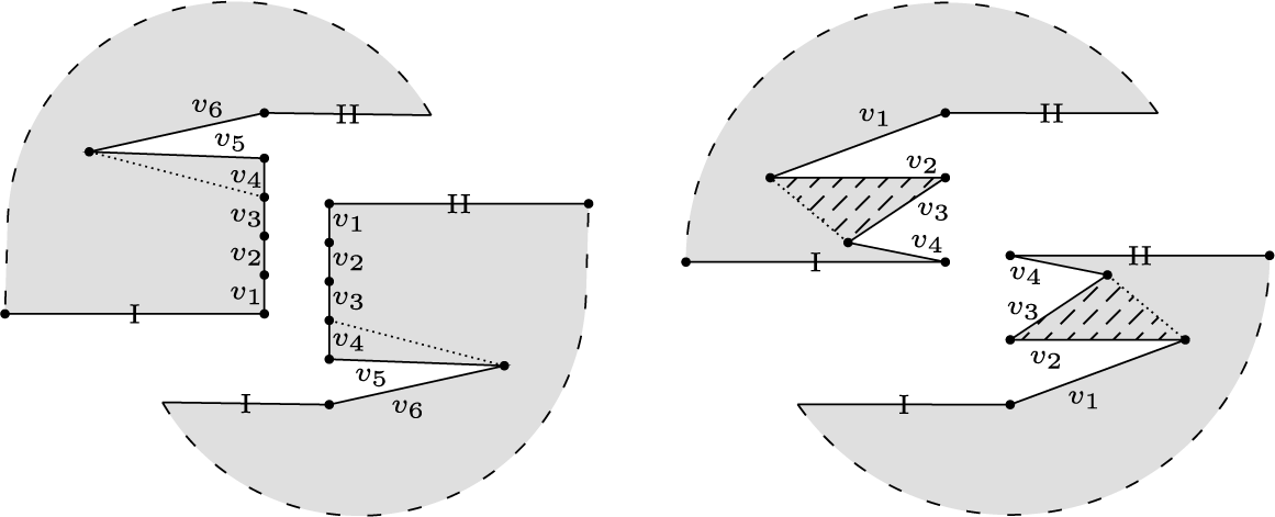
 . Furthermore, the hyperelliptic involution then necessitates that on the other domain the saddle connections are labelled
 $(v_k,\dots ,v_1)$
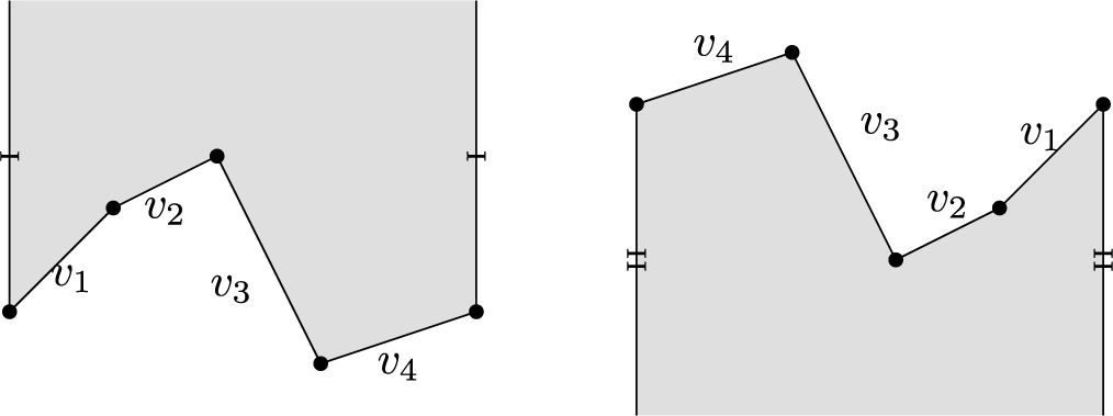
from left to right, as in Figure 1.
A hyperelliptic surface with simple poles.

If
 $(X,\omega )$
generates a Teichmüller curve M then Proposition 3.3 implies that any surface in M can only have cylinders in the same direction as the residue core curves. With the use of Lemma 3.5, we show that this rules out all possibilities outside of those stated.
Consider each pair of consecutive coordinates
 $v_i,v_{i+1}$
for
 $i=1,\dots ,k-1$
and
 $v_k,v_1$
. If the pair of coordinates are not parallel, then we have two possibilities resulting in the same conclusion. If
 $v_i+v_{i+1}$
is convex, then
 $(X,\omega )$
contains a cylinder in this direction. If
 $v_i+v_{i+1}$
is concave, then the surface
 $(X',\omega ')$
obtained by complex conjugation of the coordinates also lies in M and contains a cylinder in the direction
 $\overline {v}_i+\overline {v}_{i+1}$
. Since this direction must be parallel to the residue core curve that we have normalized to be real we have
 $v_i+v_{i+1}=a_i$
for some
 for
 $i=1,\dots ,k-1$
, and
 $v_k+v_1=a_k$
for some
 .
If a pair of consecutive coordinates are parallel, we derive a contradiction via Proposition 3.3. As not all coordinates can be parallel, assume after possibly relabelling, that we have three consecutive coordinates,
 $v_1$
and
 $v_{2}$
are parallel and not parallel to
 $v_3$
. Further, we can assume that
 $v_{2}+v_{3}$
is convex (if not, consider the conjugate surface via Lemma 3.5). Then the surface contains cylinders with core curves in directions
 $v_1+2v_{2}+v_{3}$
and
 $v_{2}+v_{3}$
which are not parallel and hence cannot both be parallel to the residue core curve contradicting Proposition 3.3.
This completes the proof that there are no Teichmüller curves in the hyperelliptic component of
 ${\Omega \mathcal M}_{g,2}(2g,-1,-1)$
as in this case
 $k=2g+1$
is odd and the above necessitates the contradiction that all
 which cannot hold for a surface that generates a Teichmüller curve.
It remains to consider the hyperelliptic component of
 ${\Omega \mathcal M}_{g,2}(g,g,-1,-1)$
for
 $g\geq 1$
. In this case
 $k=2g+2$
and by Lemma 3.5 we can assume, without loss of generality, that
 $v_1+v_2$
is convex. Then as
 $v_i+v_{i+1}$
is real for all i, necessarily
 $v_{2j+1}+v_{2j+2}$
for
 $j=0,\dots , g$
are also convex and we have
 $\sum _{j=0}^{g}a_{2j+1}=1$
. Further, after rescaling we may assume
 $\Im (v_i)=(-1)^i$
.
Let
 $\psi (t)$
be the action of the parabolic matrix with
 which fixes the imaginary part of all coordinates and acts on the real part of the coordinate
 $v_{2j+1}$
for
 $j=0,\dots ,g$
as

However,  and M is closed, hence
 is rational. The same argument after conjugation of the surface holds for
 $v_{2j}+v_{2j+1}$
for
 $j=1,\dots ,g$
and also for
 $v_{2g+2}+v_1$
. Such conditions precisely describe the linear manifolds given by the Hurwitz space
 .
3.4 Hyperelliptic components of meromorphic strata with higher order poles
Throughout this section we work in a hyperelliptic component of some signature
 $\mu $
, i.e. with one zero or two zeros of equal order and one pole or two poles of equal order, and suppose moreover that the pole order is at least two.
Proposition 3.6. Every Teichmüller curve in a meromorphic hyperelliptic stratum contains a flat surface with a cylinder.
As a first step toward this claim we prove:
Lemma 3.7. If
 $(X,\omega )$
generates a Teichmüller curve M and has a Boissy presentation where one basic domain has two saddle connections on its boundary whose homology classes are independent in M (i.e. not restricted to be parallel in M), then there is a flat surface
 $(X',\omega ') \in M$
with a cylinder.
Proof. Consider the basic domain in the Boissy presentation of
 $(X,\omega )$
that contains two saddle connections on its boundary whose homology classes are independent in M. Hyperellipticity implies that if
 $v_1,\ldots ,v_k$
for
 $k\geq 2$
are the saddle connections at the boundary of this half-plane labelled from left to right, then
 $v_k,\ldots ,v_1$
are the saddle connections at the boundary of an oppositely oriented half-plane in the Boissy presentation. If the saddle connections
 $v_i$
and
 $v_{i+1}$
for some
 $i=1,\dots ,k-1$
form two sides of a triangle
 $\Delta = \Delta (ABC)$
in the core
 , then this triangle and its hyperelliptic image gives a cylinder.
If there is no choice of
 $v_i$
and
 $v_{i+1}$
that form two sides of a triangle (i.e. the path
 $v_1,...,v_k$
is concave) then Lemma 3.5 gives that the surface obtained by conjugating all periods also lies in M. This surface and the assumption that the original domain contained saddle connections with independent directions ensures that some
 $\bar {v}_i$
and
 $\bar {v}_{i+1}$
for
 $i=1,\dots ,k-1$
form two sides of a triangle in the core of this conjugated surface. This triangle and its hyperelliptic image give a cylinder.
Coordinate dancing
The following argument to move around the saddle connections on the boundary of a Boissy presentation also relies on a path within the Teichmüller curve, but leaving the  -orbit of the initial flat surface.
Pick some saddle connection
 $v_k$
on the boundary of some Boissy basic domain and let p be the pole corresponding to the (exterior of this) domain. We write
 . Using the action of
 we may arrange that
 $v_k$
is horizontal, i.e.
 with
 $0<x_k<1$
. We now stretch the vertical direction so that
 $|y_j|>x_j$
for all j such that
 $v_j$
is not horizontal (i.e. not parallel to
 $v_k$
). We let V be this (non-empty) set of indices of (‘rather vertical’) saddle connections. Consider now the path that replaces
 by
 and more generally makes

We refer to the path as coordinate dancing. This path stays inside M since M is cut out by  -linear equations. In fact we only have to verify that those linear equations hold for the real and imaginary parts along the path. For this we observe that the real part is rescaled by a common factor, while the imaginary part is the sum of the initial imaginary part and the real part rescaled by a common factor, and for those summands the
 -linear equations hold individually.
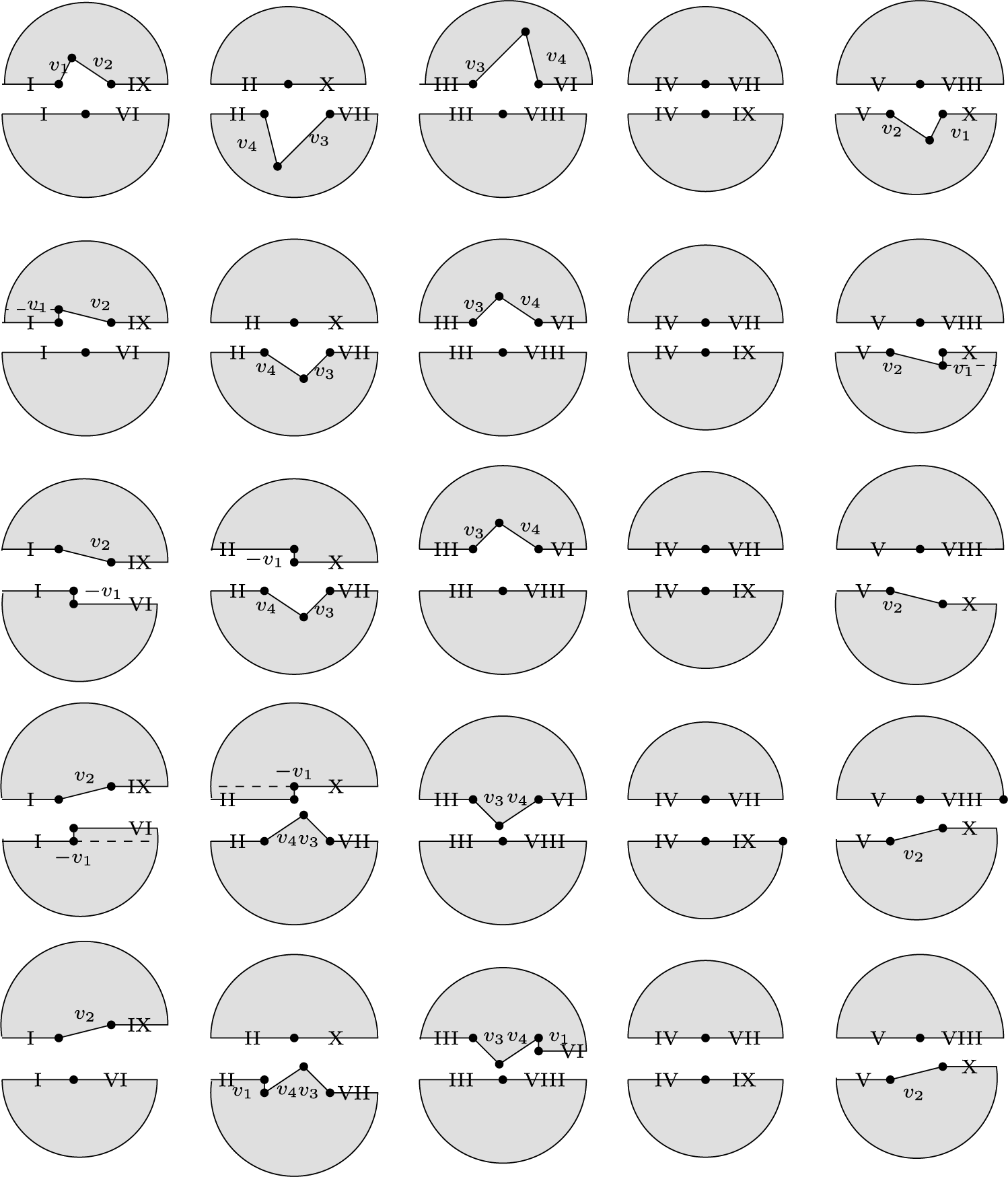
The initial phase of the dance, shrinking and rotating till
 $t=1/4$
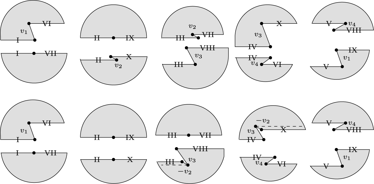
, is illustrated in the passage to the second line in Figure 2 using the saddle connection
 $k=2$
.
Dancing coordinate
 $v_2$
in the stratum
 ${\Omega \mathcal M}_{2,2}(8,-6)$
.

As illustrated in the passage between the third and fourth line of Figure 2, once
 $v_k$
passes the vertical line as we follow the dancing path, we need to cut and reglue along
 $v_k$
(and simultaneously along all boundary saddle connections that are parallel to
 $v_1$
) in order to maintain a Boissy presentation, resulting in the saddle connection
 $v_k'$
.
Actually the fourth row in Figure 2 is not quite a Boissy presentation, since some of the the saddle connections in V are ‘tilted over’. Recall that Boissy’s algorithm identifies unique local period coordinates for any surface without vertical saddle connections. Further, the algorithm returns the same coordinates for all nearby surfaces until a coordinate becomes vertical. Passing one of these coordinates through the vertical will result in Boissy’s algorithm returning a new set of local period coordinates. It is convenient for us to sometimes stay in the original coordinates even though some may have passed through the vertical or are ‘tilted over’, as our dance will immediately return these coordinates back through the vertical.
Now two cases may happen. First, none of the saddle connection parallel to
 $v_k$
touches any of the rather vertical saddle connections, as shown in the figure. (In this case the cut and reglue for the ‘tilted over’ saddle connections in the set V will be undone in the next step anyway and so we kept their position for simplicity.) We thus continue along the dancing path and arrive at the point where
 $v_k'$
passes the vertical line (fifth row in Figure 2). This requires another cut and reglue resulting in the saddle connection
 $v_k"$
.
To summarize the first case (sixth row in Figure 2): for
 $t=1$
all the boundary saddle connections in V are back to their initial position, while
 $v_k$
(and all those parallel to it) have danced to the half-plane at angle
 $2\pi $
in counterclockwise direction from their initial position.
In the second case (see Figure 3) some connection parallel to
 $v_k$
touches in the moment of tilt over a saddle connection in V. In this case we have to reglue the tilted over saddle connection to arrive at a Boissy presentation. The dancing path stops here and the sequel depends on the context.
Dancing coordinate
 $v_2$
touching in the moment of tilt over.

With our new tool in hand we proceed to prove Proposition 3.6.
Proof of Proposition 3.6.
Let
 $(X,\omega )$
be a flat surface that generates the Teichmüller curve M. We claim that there is a pole p so that among the saddle connections on the boundary of the Boissy domains adjacent to p, there are two which are
 -linearly independent in homology. Consider the global picture: each boundary saddle connection is adjacent to one or two poles. Moreover since
 $(X,\omega )$
generates a Teichmüller curve, the boundary saddle connections span a two-dimensional subspace in cohomology. Connectivity of the whole surface implies that there is some p as claimed.
Now we start coordinate dancing with one of the saddle connections adjacent to p, say v. The coordinate dance will move all coordinates that are parallel to v through the half-plane domains of their associated pole while all coordinates not parallel to v will remain on the boundary of the same half-planes. We continue this dance until one of the coordinates parallel to v arrives on the boundary of a half-plane domain containing a coordinate not parallel to v. The dance will always terminate in this way due to the choice of p and the presence of another saddle connection not parallel to v in the domains for p. There are three possibilities.
If the dance terminates when coordinates are not tilted over, then our chosen saddle connections are the Boissy coordinates and the hypothesis of Lemma 3.7 is met.
If the dance terminates when coordinates are tilted over, then these coordinates do not form the Boissy coordinates. There are two possibilities. If the angle between the dancing and non-dancing adjacent coordinate on the same half-plane domain is acute, the coordinates form a triangle and just as in the proof of Lemma 3.7, this triangle and its image under the hyperelliptic involution form a cylinder. If no angle between dancing and non-dancing coordinates is acute, we may continue the dance, rotating the dancing coordinates until the angle becomes acute and we obtain a cylinder.
Thanks to Proposition 3.6 we assume from now on that the surface
 $(X,\omega )$
that generates the Teichmüller curve has a cylinder, rotated so that its core curve is vertical, in short a vertical cylinder. We work with the generalized Boissy presentation of this surface. The geometric criterion Proposition 3.3 immediately implies that if
 $(X,\omega )$
with a vertical cylinder generates a Teichmüller curve, then all other saddle connections on the boundary of the basic domains in a generalized Boissy presentation are vertical. We refer such a presentation as a pure vertical presentation and assume this from now on.
We moreover distinguish the saddle connections on the boundaries of the building blocks. External saddle connections are the (vertical) saddle connections on the boundary of the infinite half-planes. Internal saddle connections are the remaining vertical saddle connections. They are internal to subsurfaces made out of cylinders (with vertical core curves) only.
Since the hyperelliptic involution acts on the surface, mapping Boissy’s building blocks into building blocks, it also acts on the set of external and internal saddle connections. These saddle connections are thus either invariant under the action of the involution, or exchanged in pairs.
We begin with a simple, yet useful observation regarding cylinders in hyperelliptic strata which we state as a lemma.
Lemma 3.8. In a hyperelliptic component, all cylinders are fixed by the involution.
Proof. If not, there would be a pair of cylinders exchanged by the involution. However, changing the size of one of the cylinders would destroying the existence of the involution while staying in the hyperelliptic component of the stratum.
Which leads to the following assertion.
Lemma 3.9. In a surface with pure vertical presentation that generates a Teichmüller curve there are no invariant internal saddle connections.
Proof. Any invariant internal coordinate will appear at the two ends of the same cylinder with vertical core curves. Connecting these saddle connections by straight lines across the initial cylinder will form the core curves of another cylinder. Since these crossing lines are not vertical, this cylinder together with any of the other boundary saddle connections of the vertical presentation gives the desired contradiction to Proposition 3.3 (after turning the new direction into the vertical one).
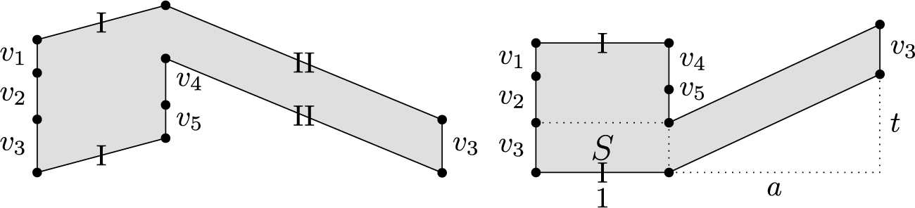
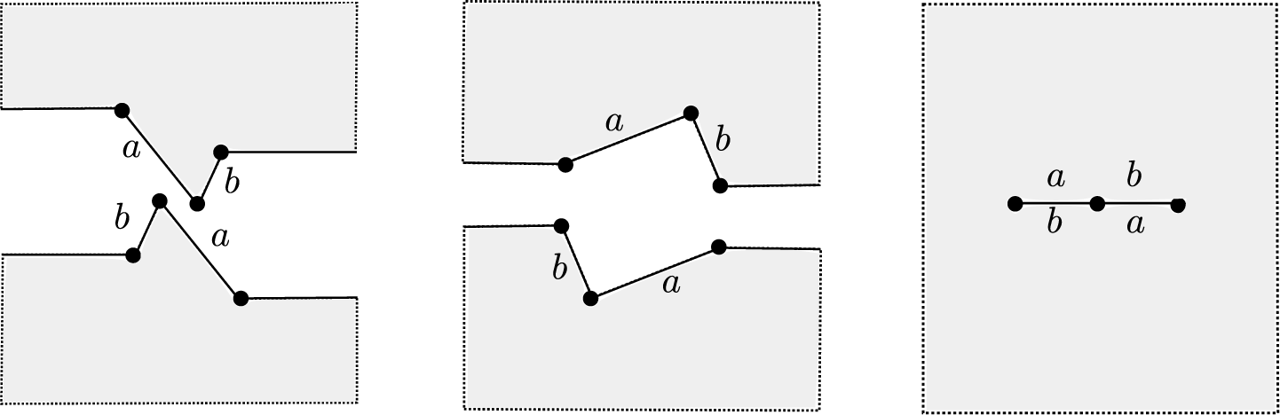
We isolate another situation favourable to prove the existence of a non-vertical cylinders: A cleaver consists of two cylinders with vertical core curves, a simple cylinder and a cylinder with two or more saddle connections, with both boundary curves of the simple cylinder glued to the boundary of the non-simple cylinder as in Figure 4 left. Elementary geometry shows:
A cleaver and its shear that exhibits a horizontal cylinder.

Lemma 3.10. A cleaver contains a cylinder with a non-vertical core curve.
Proof. Shearing by a vertical parabolic we may assume that the open ends of the non-simple cylinders are facing each other, at the expense of having a skew cleaver. By rescaling we assume that S in Figure 4 right is a unit square, the cleaver is twisted by
 $0\leq t < 1$
, and its hold has length a. Now the direction of slope
 $\lfloor t \rfloor /(1+a)$
contains a cylinder.
Lemma 3.11. A surface
 $(X,\omega )$
that contains a cylinder and generates a Teichmüller curve, given in pure vertical generalized Boissy presentation, consists only of Boissy basic domains (half-planes) and simple cylinders (at least one). The boundary saddle connections are all external, either invariant or alternatively exchanged on the two ends of a simple cylinder.
Proof. By the preceding Lemma 3.10 and our main criterion Proposition 3.3 we may exclude systems of cylinders in the complement of the half-planes that contain a cleaver. Since we excluded invariant internal saddle connections in Lemma 3.9 there are four types of cylinders in a generalized Boissy presentation that we have not yet excluded:
-
a) A simple cylinder between two external saddle connections, hence zero internal saddle connections.
-
b) Two external and at least two internal saddle connections.
-
c) At least four external and zero or more internal saddle connections.
-
d) Zero external and at least four internal saddle connections.
(It is in (d) that we can exclude cylinders with two internal saddle connections, as they will create a cleaver.) We denote by the same letter as in the list the number of such cylinders by e the number of non-invariant external saddle connections, by i the number of non-invariant internal saddle connections and by f the number of invariant (‘fixed’) external saddle connections.
We count the number of Weierstraß points. These are the pole (if unique), the zero (if unique), the f midpoints of the invariant (hence external) saddle connections, and two points in the interior of each cylinder. In fact, by Lemma 3.8, in a hyperelliptic component all cylinders are fixed by the involution. If we write Z for the number of zeros, P for the number of poles, and C for the number of cylinders, we get
 $$ \begin{align*} 2g+2 \;=\; (2-Z) + (2-P) + 2C + f\,. \end{align*} $$
Altogether we find the first of the conditions
 $$ \begin{align*}\begin{aligned} a+b+c+d &\;=\; \frac12\bigl(2g-2+Z+P-f\bigr) \\ 2a+2b+4c &\,\leq\, e \\ 2b+4d &\,\leq\, 2\bigl(2g-2+Z+P-f-e\bigr)\,. \end{aligned} \end{align*} $$
The second condition gives the count of non-invariant external coordinates, which appear in on opposite sides of the same cylinder (if adjacent to some cylinder). The third equation gives the count of non-invariant internal coordinates, each of which is counted twice. The right hand side expresses that the total number of boundary saddle connections
 $i+f+e=2g-2+Z+P$
gives a coordinate system for the stratum
 ${\Omega \mathcal M}_{g,n}(\mu )$
.
Summing twice the second and the third equation implies
 $b=c=0$
. In this situation the internal coordinates of any element in d) can only be glued to the same cylinder, since a) does not provide internal coordinates. This means that the element in d) form their own connected components. Since this is impossible, we conclude
 $d=0$
and all the claims of the lemma.
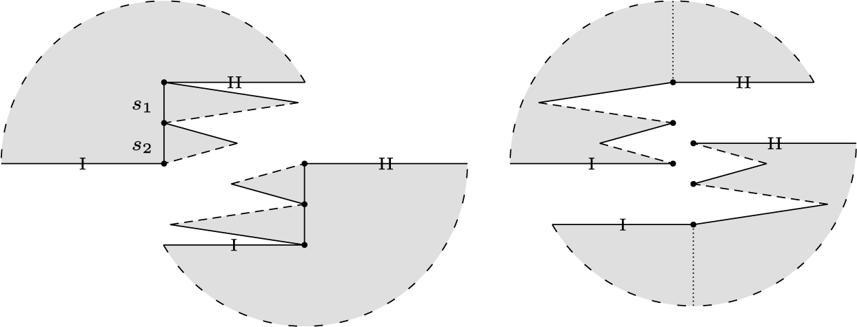
Next, we constrain how these boundary saddle connections are distributed on Boissy’s basic domains as in Figure 5, left.
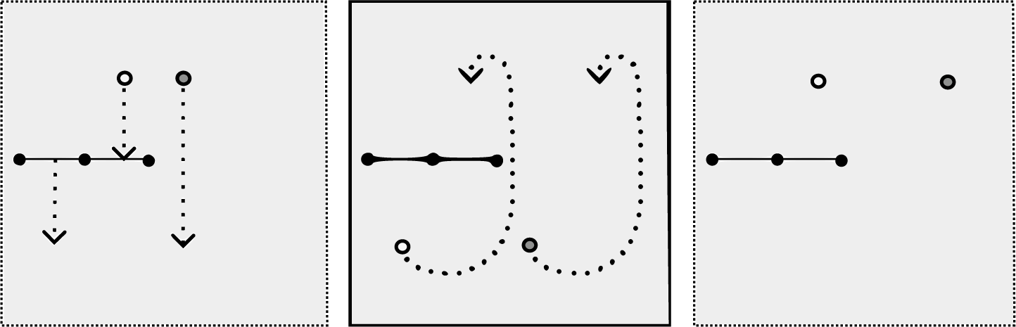
Pulling through cylinders: The surface
 $\Phi (0)$
on the left and
 $\Phi (1)$
on the right.

Lemma 3.12. The boundary of each Boissy’s basic domains has either
-
i) no boundary saddle connections, or
-
ii) only invariant external saddle connections, or
-
iii) exactly one non-invariant external saddle connection (thus bounding a simple cylinder on its other side).
Proof. Suppose some basic domain has two adjacent non-invariant saddle connections on its boundary.
Shearing by a vertical parabolic element we may assume that those simple cylinder with vertical core curves bounding the non-invariant boundary saddle connections do not have horizontal saddle connections. By cut and reglue we may present the cylinders to be twisted by less that the length of the waist curve, i.e. such that the diagonal decomposes the cylinder into two acute triangles, see the left of Figure 5. This figure also shows the new coordinates that we are using. The coordinate system no longer contains the waist curves of the cylinders
 $s_i$
, but the sides of the acute triangles
 $v_1,\ldots ,v_4$
and (if they exist) the remaining coordinates
 $v_5,\ldots ,v_n$
on the boundary of the half planes.
We consider the ‘pulling through’ path
 $\phi (t) = (X_t,\omega _t)$
as in (1). For
 $t \in [0,1]$
. This path stays within the complex two-dimensional manifold containing the
 -orbit of the initial surface. At its endpoint
 $t=1$
we construct the desired cylinder with two adjacent coordinates coming from the two adjacent cylinders. These coordinates formed a concave path in the original surface, but after pulling through now form a convex path and hence a triangle which with its image under the hyperelliptic involution forms a cylinder. This situation is presented on the right of Figure 6. Proposition 3.3 applies after rotating the direction of the cylinder to the vertical and identifying that first and final coordinates on the domain are not parallel to each other (
 $v_1$
or
 $v_4$
in Figure 6 on the right) and hence at least one will be external and not parallel to the new cylinder direction, providing the contradiction.
Finding cylinders.

The other case to rule out is (at least) one simple cylinder (with its adjacent) non-invariant external saddle connections next to some invariant external saddle connection. By ‘pulling through’ as in the previous case we arrive at the configuration with the one new coordinate from the cylinder adjacent to a non-invariant saddle connection forming a convex path and hence a triangle. This triangle and its image under the hyperelliptic involution form a cylinder. This is depicted in Figure 6 on the left, where coordinates
 $v_5$
and
 $v_4$
form the triangle. Proposition 3.3 applies after rotating the direction of the cylinder to the vertical and identifying that the other new coordinate coming from the cylinder (
 $v_6$
in Figure 6 on the left) is not parallel to the direction of the cylinder.
Rotate again for the next dance
So far, for Lemma 3.12 we have been using the generalized Boissy presentation, i.e. admitting cylinders with vertical core curves. In order to get further constraints on the periods of the saddle connections we have to use again paths in the linear manifold that leave the  -orbit, i.e. dancing paths or a variant of it. For this purpose consider a surface with in Lemma 3.12 and pull through the cylinders, like in Figure 5 right (but with only one cylinder or one invariant external saddle connection per basic domain). Cutting the basic domains open along vertical lines at the end of the broken line of saddle connections (the dotted lines in Figure 5 right), regluing along the infinite horizontal separatricies and rotating the picture by
 $\pi $
gives a flat surfaces in (standard) Boissy presentation that we use next.
Lemma 3.13. Suppose the surface
 $(X,\omega )$
in the presentation of Lemma 3.12 has an invariant external saddle connections (as in (ii) of that lemma). Then the Teichmüller curve generated by
 $(X,\omega )$
is one of the obvious cases from Proposition 2.2 (iii a) or (iii b) covering surfaces with residues conditions.
Proof. We may assume by Proposition 3.6 that there is at least one cylinder. We pull this cylinder through and rotate for the next dance, as described above. We select one of the invariant external saddle connections
 $v_1$
to apply the coordinate dancing. Since
 $(X,\omega )$
generates a Teichmüller curve, all the invariant external saddle connections are parallel and hence dance simultaneously and if there are several of them adjacent to one Boissy domain, they dance (i.e. move between the Boissy domains) together. This dance will terminate in one of two ways:
The first possibility is that a set of invariant coordinates appears on a basic domain with two pulled-through coordinates at the end of a certain number of full dancing paths (i.e., full rotations
 $2k\pi $
for some
 ). Pulling the coordinates back through to obtain a cylinder we obtain a contradiction to Lemma 3.12 as this Boissy domain will have a non-invariant external saddle connection (due to the cylinder) and at least one invariant external saddle connection (the danced coordinate(s)).
The second possibility is the dance ends the moment the cylinder coordinates are tilted over (i.e., rotations by
 $(2k+1)\pi $
for some
 ). One pulled-through coordinate and the adjacent invariant coordinate now form a cylinder formed by
 $v_2$
, the dancing coordinate
 $v_3$
, the dashed line and the hyperelliptic image of this triangle in both cases of Figure 7.
Dancing the invariant coordinate
 $v_3$
ends tilted over.

First, if any of the danced invariant coordinates now lie alone on a Boissy domain (as
 $v_4$
on the left of Figure 7) we obtain a contradiction as their direction lies outside the direction of the waist curves of the newly formed cylinder. Second, if there were any Boissy domains containing two or more invariant external coordinates (as for example on the right of Figure 7) we also obtain a contradiction as a pulled-through coordinate and the adjacent invariant coordinate now form a cylinder and the second invariant coordinate is outside of the direction of the waist curves of the new cylinder.
Finally we are left in the local situation where a single invariant coordinate has danced to a domain where the pulled through coordinates are tilted over (i.e., rotations by
 $(2k+1)\pi $
for some
 ). The danced invariant coordinate now forms a cylinder with the adjacent pulled through coordinate and the waist curve of this cylinder is in the direction of the other pulled through coordinate. This configuration with the configuration of original surface is enough to describe the local equations on these coordinates.
Let
 $v_2$
and
 $v_3$
be the saddle connections that have been pulled through. On the original surface
 $v_2 + v_3$
is the waist curve of the cylinder, so there must be a relation
 for some
 , since otherwise Proposition 3.3 provides a contradiction. (Recall that in a generalized Boissy domain our convention is that the direction of vertical saddle connections is up.) At the end of the dance (an odd number of rotations by
 $2\pi $
) we obtain
 $-v_1 + v_2$
as the waist curve of a cylinder (possibly after changing the role of
 $v_2$
and
 $v_3$
). This implies that
 and thus (possibly changing the orientation of
 $v_1$
) we find
 $s=1$
.
We now consider the surface globally. As discussed, if there were any more invariant coordinates they cannot appear at the end of the dance in their own basic domains as this would form a contradiction. Similarly, if there were any other pulled-through coordinates they will now appear in “tilted-over” position. Proposition 3.3 will provide a contradiction unless one of the pulled-through coordinates is now parallel to the waist curve of the new cylinder (that is, to
 $v_3$
) and the other pulled through coordinate forms a new cylinder with an invariant coordinate that has danced onto this basic domain with necessarily parallel waist curve to
 $v_3$
.
Labelling these coordinates
 $u_1,u_2,u_3$
consistently with the
 $v_i$
we find
 $u_1$
and
 $v_i$
are parallel and in fact,
 $u_i= kv_i$
for some
 $k>0$
. Hence we have the saddle connections come in sets of three that are real scaled copy of
 $(v_1,v_2,v_3)$
and it remains to compute the comparison factor k for each set.
Now we label the (even number) Boissy domains adjacent to a poles in counterclockwise order, starting with a pulled-through cylinder on domain number one. Since the ‘first possibility’ above provided a contradiction, the first Boissy domain with an invariant saddle connection has an even number. Rotating in the other direction we find the the next Boissy domain with pulled-through cylinders sits on a Boissy domain with an even number and inductively we see that this parity constraint holds for all cylinder and all invariant saddle connections. Comparing the triples of saddle connections for a pulled-through cylinder and an invariant saddle connection for clockwise and counterclockwise dancing implies that all pairwise comparison factors (denoted by k above) are equal to one, i.e. any two invariant saddle connections and any two cylinders have the same geometry.
The parity constraint for the Boissy domains containing a (don’t pull it through!) cylinder implies that the cylinders cannot connect Boissy domains adjacent to the same poles. Consequently, there are precisely two poles since we are in a hyperelliptic stratum.
The parity constraint (together with the length agreements that follow from
 $k=1$
) also implies that the map stacking all the cylinders on top of each other (or equivalently all the invariant external saddle connections on top of each other) extends to a well-defined covering map. Depending on the degree of the map we are in case (iii a) or (iii b).
Lemma 3.14. Suppose a Teichmüller curve M in a hyperelliptic component of a stratum with non-simple poles contains no surfaces in the presentation of Lemma 3.12 with an invariant external saddle connections (as in (ii) of that lemma). Then M is one of the obvious cases from Proposition 2.2 (i a), (ii a), or (ii b).
Proof. We may assume by Proposition 3.6 that there is a surface
 $(X,\omega )$
that generates M and has at least one cylinder. By assumption, this surface also has no invariant saddle connections in the direction of this cylinder. We pull the cylinders in this direction through and rotate for the next dance, as described previously. The situation is illustrated in the first row of Figure 8. We now select a steepest saddle connection
 $v_i$
for dancing, i.e., one for which
 is maximal. The dancing path is easier to visualize if we normalize this coordinate to be vertical at the start of the dance (see the coordinate
 $v_i$
in the second row of Figure 8), as opposed to horizontal in the original coordinate dancing. (In fact with this choice any saddle connection not parallel to the selected one will remain adjacent to its initial basic domain throughout the dance.) We stretch sufficiently in the horizontal direction (such that
 for all k with
 $v_k$
parallel to
 $v_i$
and for all j in the complementary set H of (’rather horizontal’) saddle connections).
Dancing the steepest saddle connection.

Now we rotate  while modifying slightly the periods of the saddle connections so as to stay in M, just as in (2) with the role of real and imaginary part swapped. The dancing procedure is illustrated in the remaining rows of Figure 8). It ends once the selected saddle connection appears on the same basic domain as some other saddle connection. If a dancing coordinate arrives on a domain with two coordinates (two pulled through coordinates, both were not parallel to the coordinate we chose to dance) we obtain a contradiction in the two possible cases.
The first possibility is that the dance terminates after a certain number of full dancing paths (i.e., full rotations
 $2k\pi $
for some
 ). Then our coordinates are in Boissy configuration and we may pull back through the two pulled through coordinates to reform the cylinder. The waist curve of this cylinder is not fixed to be parallel to
 $v_i$
, the danced coordinate, hence we obtain a surface that contradicts Proposition 3.3.
The second possibility is that the dance terminates when the pulled through cylinder coordinates are tilted over (i.e., full rotations
 $(2k+1)\pi $
for some
 ). In this case the danced coordinate and the adjacent pulled through coordinate now form a cylinder. To avoid a contradiction with Proposition 3.3 the other pulled through coordinate must be parallel to the waist curve of the new cylinder. But then rotating such that this direction is vertical, this coordinate becomes an invariant coordinate contradicting our assumption that no surfaces in M are of this form.
Hence the dance must terminate with a dancing coordinate on a domain with just one other coordinate. However, this means that the other coordinate that originated on this domain must have danced and was hence parallel to our steepest saddle connection. If that saddle connection now lies in a domain by itself we obtain a contradiction as we obtain a cylinder (after possibly pulling-through) with waist curve not parallel to this saddle connection. Hence this saddle connection coordinate must have danced to a domain with exactly one other saddle connection. However, this means a saddle connection that originally lay on this domain must have danced. Chasing this argument around the surface we see that every cylinder contributed a pulled-through saddle connection that danced and hence was parallel to the selected saddle connection.
Label the saddle connections
 $v_1,\ldots ,v_d$
where
 $d=2g+|\mu |-2$
such that
 $v_{2j-1}$
and
 $v_{2j}$
for
 $j=1,\ldots ,d/2$
are the pulled-through coordinates from each cylinder from left to right on the upper basic domains, and such that the dance results in
 $v_{2j-1}$
appearing on the domain with
 $v_{2j+2}$
(considering the indices modulo d). Our argument above gives
 $v_{2j-1}=k_jv_1$
for
 and
 $j=2,\ldots ,d/2$
. The same argument dancing instead saddle connections in the direction such that
 is minimal gives
 $v_{2j}=\ell _j v_2$
for
 and
 $j=2,\ldots ,d/2$
.
In
 $(X,\omega )$
the waist curves were necessarily parallel and hence imposed the condition that
 $v_{2j-1}+v_{2j}=m_j(v_1+v_2)$
for
 . Similarly, after dancing we create cylinders by pulling through which implies
 $v_{2j-1}+v_{2j+2}=n_j(v_1+v_4)$
for
 and
 $j=1,...,d/2$
.
The only solution to these equations is
 $k_j=l_j=m_j=n_j=1$
for all j. Thus all the flat surfaces parametrized by M admit a cover onto a flat surface with just two saddle connections on the boundary of the Boissy domains. Hence the Teichmüller curve generated by
 $(X,\omega )$
is one of the obvious cases as listed in the proposition, the cases being distinguished by the number of zeros (and poles) in the range of the covering map and the degree of the cover.
The proof of Theorem 1.1 is complete as a combination of Proposition 3.4 in Section 3.3 and the series of lemmas in this Section 3.4.
Appendix: An -linear non-algebraic manifold
 -linear non-algebraic manifold
by Benjamin Bakker and Scott Mullane
An  -linear manifold is a submanifold of a stratum of differentials defined locally by homogenous real linear equations in period coordinates. They hold great importance stemming from a diverse range of connections including billiards in polygons, Jacobians with real multiplication, and dynamical rigidity. In this appendix, we present a simple example of
 -linear manifold in a meromorphic stratum that is not algebraic, hence showing the algebraicity of these loci in holomorphic strata [Reference Filip11] does not extend to the meromorphic case.
For
 $\mu =(m_1,\dots ,m_n)$
an integer partition of
 $2g-2$
, the stratum of differentials of type
 $\mu $
is the moduli space of flat surfaces or pairs of pointed smooth curves and meromorphic differential of type
 $\mu $
, set theoretically,
 $$ \begin{align*}\Omega\mathcal{M}_{g,n}(\mu):=\{(X,\omega,p_1,\dots,p_n)\hspace{0.1cm}|\hspace{0.1cm}(X,p_1,\dots,p_n)\in\mathcal{M}_{g,n}, \hspace{0.1cm} (\omega)_0-(\omega)_\infty=\sum m_ip_i\}.\end{align*} $$
While the strata inherit an algebraic structure as a stratification of the Hodge bundle, integrating the differential
 $\omega $
yields a presentation of X, punctured at the poles of
 $\omega $
, as polygons in the complex plane with parallel side identifications. Hence we obtain a complex analytic orbifold structure locally at a point from a choice of basis for the relative homology
 , where Z and P are the zeros and poles of
 $\omega $
respectively. This basis extends locally via the flat connection and local orbifold coordinates known as period coordinates are obtained by integrating the differential by this basis.
For example, Figure 9 contains polygon presentations for three different flat surfaces in the stratum
 $\Omega \mathcal {M}_{1,2}(2,-2)$
. In this case, both Z and P are one-point sets and a flat surface in the stratum can be expressed by two broken half-planes with parallel side identifications as follows. The pairs of line segments a and b are identified as labeled and the two infinite half rays extending to the left and the two infinite half rays extending to the right are identified respectively. This gives one vertex with cone angle
 $6\pi $
, the unique double zero of the differential, and the surface is punctured at infinity, the unique double pole of the differential. Varying a and b in
 with the condition
 $\Re (a),\Re (b)>0$
, provides period coordinates for a local chart in the stratum
 $\Omega \mathcal {M}_{1,2}(2,-2)$
. The flat surface on the right in Figure 9 is obtained by setting
 $a=b=1$
in this chart and identifying the infinite half rays. The polygon presentation for this flat surface is then the infinite plane with two slits with opposite sides identified as labeled.
Three flat surfaces in
 $\Omega \mathcal {M}_{1,2}(2,-2)$
.

Now consider the stratum
 $\Omega \mathcal {M}_{1,4}(2,-2,0,0)$
obtained by further allowing two phantom zeros and let
 $\pi $
be the forgetful map to
 $\Omega \mathcal {M}_{1,2}(2,-2)$
that forgets these two points. We obtain period coordinates for the fibre of
 $\pi $
over the flat surface on the right in Figure 9 as
 where
 $\Delta $
denotes the diagonal, we identify a and b with the open real intervals
 $(0,1)$
and
 $(1,2)$
respectively, and
 $(u,v)$
are the periods to the two phantom zeros from the left end of the double slit. Setting
 $u-v=1$
we obtain a local
 -linear condition and we are left to consider the closure. The only monodromy is obtained by passing the phantom zeros through the passage of slits, that is, the coordinates
 $(u,v)$
change as a point passes through the passage
 $(0,1)\cup (1,2)$
. For example, Figure 10 shows how the the loci
 $u-v=k$
and
 $u-v=k+1$
are connected for any
 and
 $k\ne -1$
. Further, the loci
 $u-v=-1$
and
 $u-v=1$
are connected by passing both phantom zeros through the slits simultaneously. Hence we obtain an irreducible
 -linear manifold
 $\mathcal {T}$
in the stratum
 $\Omega \mathcal {M}_{1,2}(2,-2,0,0)$
as the
 -orbit of the loci cut out by
 .
Inside the linear manifold
 $\mathcal {T}$
.

However, the forgetful map factors as
 $\pi =\pi _1\circ \pi _2$
through the stratum with just one phantom zero, that is, forgetting first
 $p_4$
and then
 $p_3$
:
 $$ \begin{align*}\Omega\mathcal{M}_{1,2}(2,-2,0,0)\xrightarrow{\pi_1} \Omega\mathcal{M}_{1,2}(2,-2,0)\xrightarrow{\pi_2} \Omega\mathcal{M}_{1,2}(2,-2)\end{align*} $$
Fixing
 $a=b=1$
and
 and allowing v to vary in
 we obtain a fibre of
 $\pi _2$
which is hence algebraic. However, this fibre intersects
 $\mathcal {T}$
in infinitely many points given by
 $u=c$
,
 $a=b=1$
,
 $v=c+k\ne 0,1,2$
for
 contradicting the algebraicity of
 $\mathcal {T}$
.
Acknowledgements
We thank the referee for useful suggestions.
Competing interest
None.
Data availability statement
None.