Background—global changes in a fast changing world

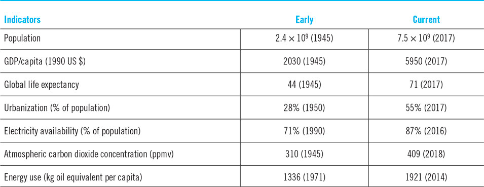
One of the three discussion points in my previous publication in this journal^{Reference Tomkiewicz1} was focused on the efforts of the Anthropocene Working Group (AWG), an interdisciplinary body of scientists and humanists working under the umbrella of the International Commission on Stratigraphy (branch of Geology) that was tasked with developing proposals for the formal ratification of the Anthropocene as an official epoch amending the Geological Time Scale. Since then, a group of 26 scientists reported on reaching their conclusions and submitted their recommendations to the Working Group at the 35th International Geological Congress in Cape Town, South Africa, in August 2016.^{Reference Zalasiewicz, Waters, Summerhayes, Wolfe, Barnosky, Cearreta, Crutzen, Ellis, Fairchild, Gałuszka, Haff, Hajdas, Head, Ivar do Sul, Jeandel, Leinfelder, McNeill, Neal, Odada, Oreskes, Steffen, Syvitski, Vidas, Wagreich and Williams2} The majority of the committee favors the mid 20th century to be the dividing line between the Holocene and the Anthropocene with the radioactive nuclei that result from the first nuclear testing to serve as a long lasting markers for the boundary. More recently, the IPCC in its latest report³ (http://IPCC.ch/reports/SR15) decided to adopt the designation as the epoch of the anthropogenic climate change. Table 1 provides a quick summary of some of the major anthropogenic changes that took place since the mid 20th century.

Table 1.

Changes in some key global indicators from the mid. 20th century to present.⁴

The proposed timeline corresponds to a single lifetime (including that of the author of this article). Effective mitigations of the ever-increasing anthropogenic damage requires understanding of the global driving forces that lead to these changes on a level that makes effective mitigation possible. The only global structural units that presently are empowered with sovereignty are individual states. Present global international organization such as the United Nations are subject to rules that are consistent with these sovereign limitations although power and wealth are playing their role to make some countries more sovereign than others.

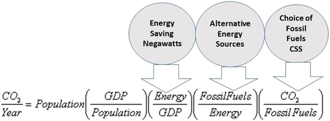
My previous review^{Reference Tomkiewicz1} was focused on analysis climate change aspects of sustainability through emphasis on the Kaya-IPAT identity. The analysis followed earlier analysis by Green et al.^{Reference Green, Espinal, Traversa and Amis5} and expanded on the mitigation potentials of the energy use terms as depicted in Fig. 1 that is reposted below. This review will continue this process with emphasis on two intensities that are embedded in this identity—the energy intensity term defined as energy/GDP and the carbon intensity. While energy intensity is almost always defined in terms of energy/GDP, carbon intensity can be defined both in terms of energy (CO₂/energy) or in terms of GDP (CO₂/GDP). In this article, unless otherwise specified, it always refers to CO₂/GDP.

Figure 1.

The Kaya-IPAT expanded identity of carbon dioxide emission out of burning fossil fuels.^{Reference Tomkiewicz1}

As was mentioned previously,^{Reference Tomkiewicz1} the Fifth Assessment IPCC Report (AR5)⁶ analyzed the global contributions of the various terms in Fig. 1, through analysis of their contributions to decadal intervals from 1971 to 2010. The two dominant terms in the identity throughout this period are the GDP/capita and the population. The three technology terms in Fig. 1 were analyzed through the energy intensity of GDP and the carbon intensity of energy—both contributing to reduction of the impact but well short of compensating for the increase cause by the first two terms.

The trigger for the work that will be described in the next section came from an informal analysis (Tomkiewicz M: http://climatechangefork.brooklyn.cuny.edu/2018/02/27/ Primary energy^{Reference Tomkiewicz7}) that was part of a series of blogs that tried to characterize the global progress of some key climate change indictors through progress of the 12 most populated countries. That compilation showed that, within a factor of 2, both the carbon intensity and the energy intensity (both in terms of GDP) are constant, independent of population or GDP/capita. It was interesting to analyze if these will be retained with a full global analysis when GDP/capita can vary by more than two orders of magnitude and the population varies by close to four orders of magnitude. The data are based on the World Bank database.⁴

Global parametrization of energy intensity and carbon intensity

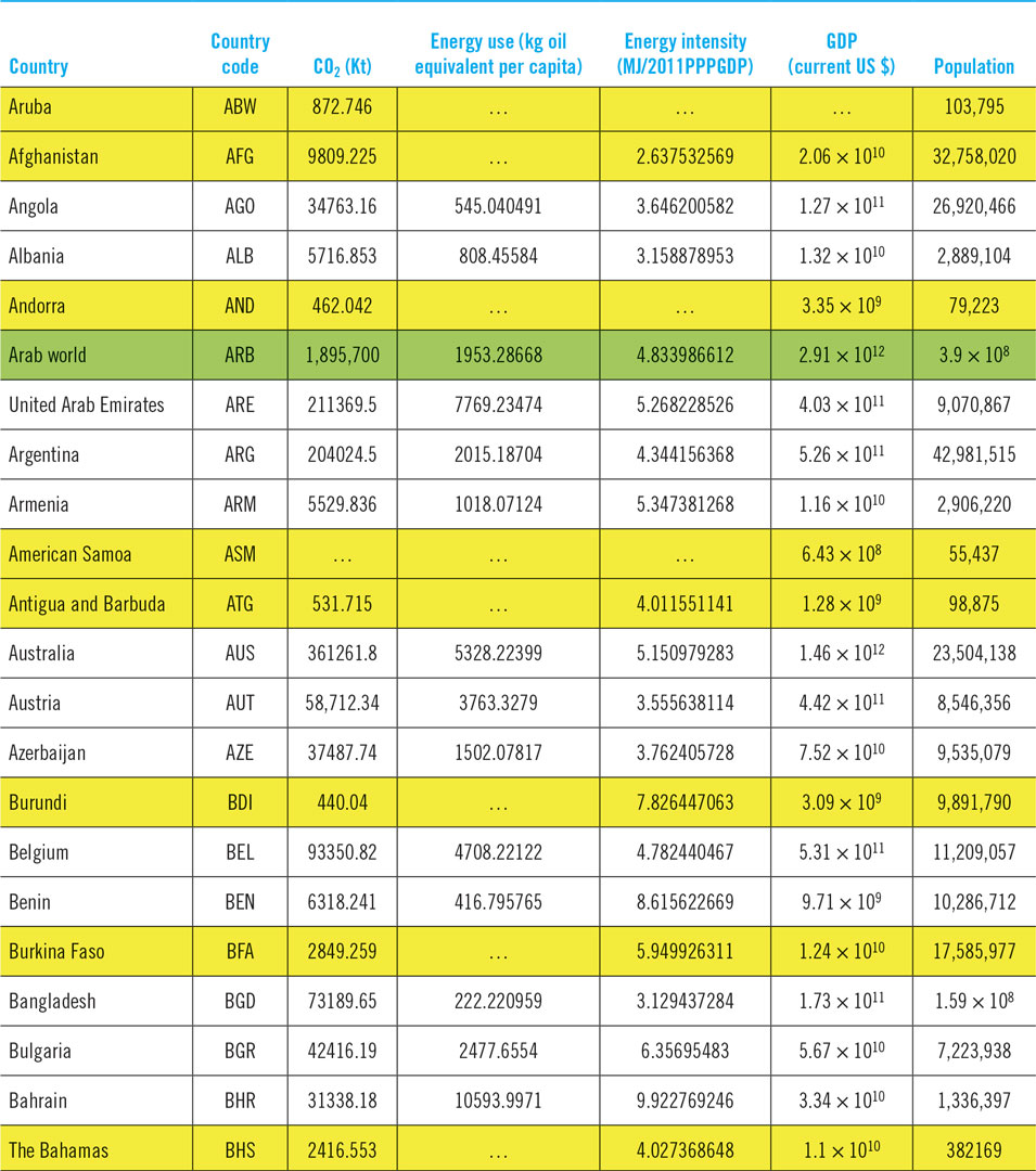
A small section of the World Bank data for 2014 is shown in Table 2. The total number of entries in the original table was 263. Other entries are of regions (Arab World in the example in Table 2). Some of the entries did not have the complete information about required indicators (Aruba, Afghanistan, Andorra, American Samoa, and Antigua and Barbados in Table 2). These incomplete entries were removed and the regions were counted separately. The final list of countries that were used includes 130 countries. The most populated countries in the list are China with population of 1.4 × 10⁹ and India with population of 1.3 × 10⁹. The least populated listed country was Iceland with population of 330,000. The most affluent country per capita (in US $ in current value) was Qatar with 87,000 US $/capita while the least affluent country in the list was Niger with GDP/capita of 430 US $. These were the only criteria for rearranging the original data. I did not care if the country is truly sovereign. I did retain the original World Bank column for energy intensity but I used it only as a reference for comparison since it was compiled with the United States PPP (purchasing power parity) $. The US $ values in this article are all current values. All the energy units were changed to millions of Joules (MJoules) and the units for the carbon dioxide were changed to kg.

Table 2.

Small section of the relevant World Bank data for 2014.

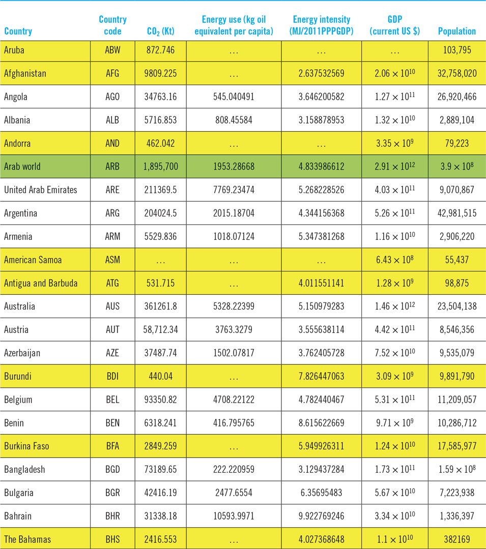
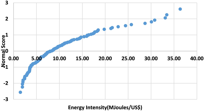
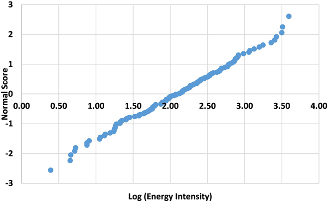
Figure 2 shows an example of testing the energy intensity data for normal distribution by using the normal probability plot (P–P plot). It is clearly not a normal distribution. However, the data converge to a clear pattern. Considering that the data represent such large differences in the two most important socioeconomic indicators that are responsible for carbon dioxide emission, it is already a sign for convergence that will be further discussed toward the end of the article.

Figure 2.

Testing for normal distribution of the energy intensity.

Figure 3 shows the corresponding P–P plot testing of the energy density to lognormal distribution. It clearly shows a good fit throughout the range.

Figure 3.

Testing for lognormal distribution of the energy intensity.

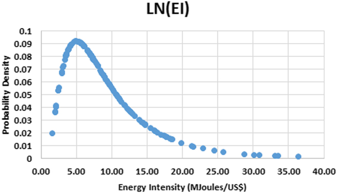
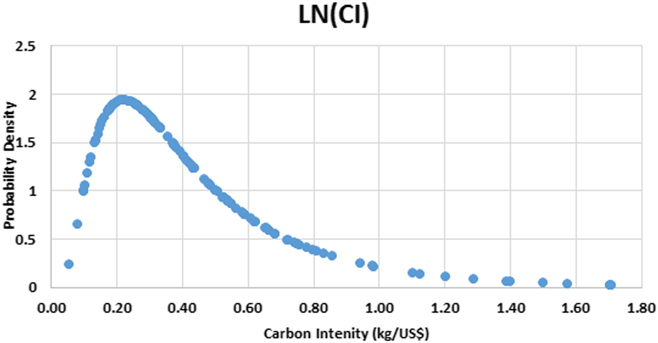
Figures 4 and 5 show the fits to lognormal distributions of both the energy intensities and the carbon intensities, both intensities with respect to the GDP.

Figure 4.

Lognormal distribution of the energy intensity.

Figure 5.

Lognormal distribution of the carbon intensity.

The probability density function (PDF) of the lognormal distribution is given in Eq. (1) as a function of two parameters, μ and σ are respectively the mean and the standard deviation of the variable natural logarithm,

(1)$${\rm{PDF}} = {1 \over {x\sigma \sqrt {2\pi } }}{{\rm{e}}^{ - {{{{\left( {{\rm{Ln}}\left( x \right) - \mu } \right)}^2}} \over {2{\sigma ^2}}}}}.$$

The mean (m) and variance (v) of the nonlogarithmic function relate to μ and σ through the following relations:

(2)$$\mu = {\rm{\ Ln}}\left( {{m / {\sqrt {\left( {1 + {v / {{m^2}}}} \right)} }}} \right),$$

(3)$${\sigma ^2}{\rm{\ }} = {\rm{\ Ln}}\left( {1 + {v / {{m^2}}}} \right).$$

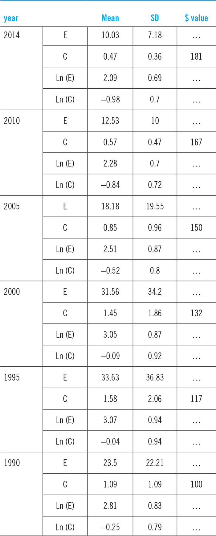
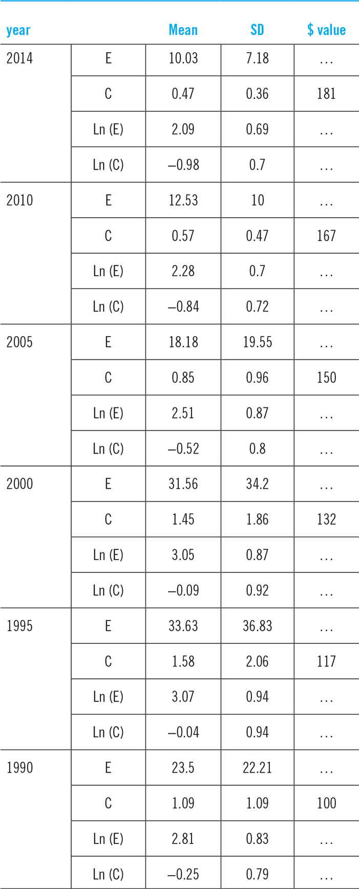
The values for the four parameters for multiple years starting with 1990 shown in Table 4.

Lognormal distributions have long history in science and social sciences.^{8,Reference Limpert, Stahel and Abbt9} I chose an amusing one published by Kay Sun^{Reference Sun10} with its associated reference:

1. (i) Concentration of elements and their radiation in the Earth’s crust^{Reference Razumovsky11–Reference Malance, Gaidolfi, Pessina and Dallara13}

2. (ii) Latent periods of many infectious diseases^{Reference Kondo14}

3. (iii) Survival time after cancer diagnosis^{Reference Boag15–Reference Horner17}

4. (iv) Abundance of species in a plant or large communities^{Reference Preston18–Reference Magurran20}

5. (v) Number of words per sentence for writers^{Reference Williams21}

6. (vi) Age of marriage for women in Denmark^{Reference Preston22}

7. (vii) Family size in England and Wales^{Reference Allanson23}

8. (viii) Size of drops in mayonnaise^{Reference Limpert, Stahel and Abbt9}

9. (ix) Size of holes in cocoa press cake^{Reference Limpert, Stahel and Abbt9}

It nice to be able to include the nations of the world in the list.

Both, the normal distribution and the lognormal distribution are used to describe random variations.^{Reference Limpert, Stahel and Abbt9} Both forms of variability are based on a variety of forces acting independently of one another. The major difference according to Limpert et al.^{Reference Limpert, Stahel and Abbt9} is that the effect can be additive or multiplicative. A good example provided by these authors is a play with two ordinary dice numbered 1–6. The total range with addition of the two dice 1 s 2–12 that can be represented by 7 ± 5 and is symmetric. If on the other hand one plays with multiplying the dice one will be playing with a more extended range of 1–36 with a highly skewed distribution.

For us is an opportunity to analyze the forces in play.

International conferences for sustainable developments always held the balance between economic development and long-term sustainability as a central objective of such meetings.²⁴ The energy and carbon intensities with respect to GDP that we are investigating here represent such a balance in their definition. However, the fact that such a divergence in the socioeconomic characteristics fit into a well-characterized distribution has the down side that may suggest, that at least for these indicators, the socioeconomics characteristics do not play a significant role or at least that the energy use and emissions are to a degree balanced throughout the broad socioeconomic spectrum. The next section attempts to examine this aspect.

The socioeconomic role

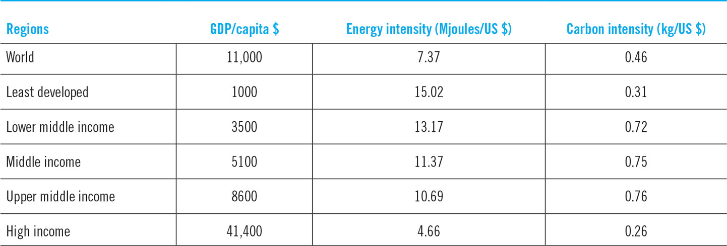
The World Bank database offers a way to investigate the dependence of the energy intensity and the carbon intensity with respect to GDP against the GDP. The database divides the World according to its GDP and monitors the same indicators as the one it monitors for countries. Table 3 shows the five regions with their average GDP/capita and their energy and carbon intensities with respect to GDP for 2014.

Table 3.

Socioeconomic indicators of the World Bank regions⁴ (2014).

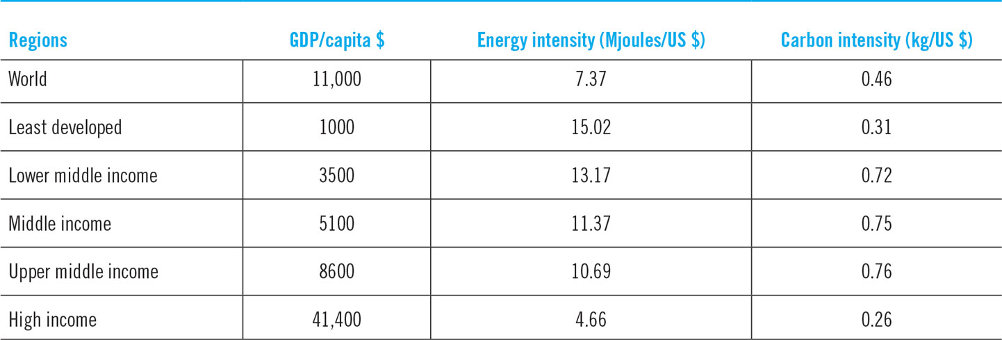
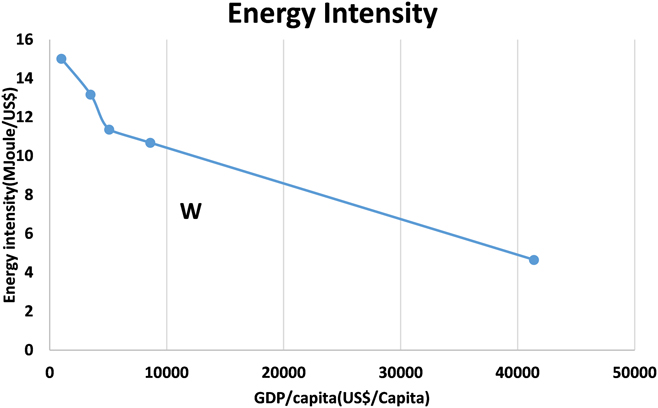
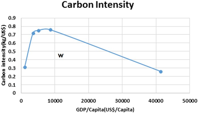
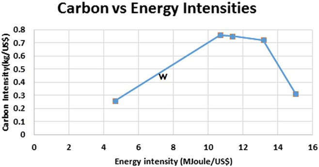
Figure 6 shows the dependence of the energy intensity on the GDP/capita with the global value superimposed (marked as w in the curve). Figure 7 shows the corresponding data for the carbon intensity and Fig. 8 shows the dependence of the carbon intensity as a function of the energy intensity.

Figure 6.

Energy intensity of the 2014 World Bank regions as a function of GDP/capita. Least developed region on the far left and high-income region on the far right. w is the global value.

Figure 7.

Carbon intensity of the 2014 World Bank regions as a function of GDP/capita. w is the global value.

Figure 8.

Carbon intensity as a function of energy intensity of the 2014 World Bank regions. w is the global value.

Figure 6 shows a consistent trend of the energy intensity to decline as a function of the GDP. This trend is common to all the region with sharpest decline in the poorer regions as compared with the richer one. As was mentioned earlier in this article, the IPCC in its Fifth Assessment IPCC Report (AR5)⁶ analyzes the global contributions of the various terms in Fig. 1, through analysis of their contributions to decadal intervals from 1971 to 2010, found a consistent global decline in energy intensity with time. Our finding indicates that the decline with time is consistent with global GDP increase.

More interesting finding is the one shows in Figs. 7 and 8. A maximum in carbon intensity is observed as a function of GDP and as a function in energy intensity. The maximum in the carbon intensity as observed in Fig. 7 is consistent with an “Environmental Kuznets curve”, forms of pollution and national income that follow an inverse U-shaped pattern, rising initially, peaking, and then declining. Such a pattern resembles the time series of income inequality described by Kuznets.^{Reference Kuznets25–Reference Hank Hilton and Levinson27}

Recent history

Table 4 shows the time dependence of the mean and standard deviation of the energy and carbon intensities, and their corresponding logarithmic expressions, from 1990 to 2014 in five-year intervals. In all cases, the analysis of the World Bank data followed the same procedure as was described earlier for 2014. Since both indicators include GDP values that change with time, I have added a column of the US $ value normalized to its value in 1990. The full distribution of these indicators was not investigated. To compare the mean and standard deviations at different times all have to be multiplied by the corresponding $ value. In all cases, the distribution covers countries with similar variability to the one described earlier for 2014 and in all cases, and for both indicators, the standard deviation is approximately the same value as the mean suggesting that the conclusions reached earlier for 2014 will be valid throughout.

Table 4.

Time dependence of the distribution parameters.

Conclusions, ramifications, and opportunities

Climate change mitigation is driven by balance of interests that often looks to be in conflict. The conflict between the economic development and energy used to drive the economic development and the choice of fuels used to supply the energy are the center of the issue. Additional conflicts are the local (state) driving forces for economic growth and the global emissions that directly or indirectly impact global climate and fresh water supply that can hinder growth. This work is trying to resolve some of these conflicts. To quote one of the readers of the article: “The author offers the observations that carbon and energy intensities are only weakly dependent on GDP and population. As universal and time-invariant constants, these intensities could help de-couple physical and human factors in the time evolution of global sustainability”. I could not have said it better. The two intensities offer promising connections between the physical environments, through their carbon and energy terms, and the socioeconomic environment, through the GDP terms, on the level of countries (sovereign and some not sovereign). Attempts to resolve some of the conflicts that were mentioned earlier should both focus on the science and technology and on the global environment in which we all live. In my earlier article in this journal ⁽¹⁾, I wrote the following: “I will argue here that the interdisciplinary nature of materials science needs now to be expanded to take the form of a connecting link between its traditional foundations in physics, chemistry, and engineering to become the link between relevant parts of these disciplines and the human environment in which we live. This journal is a testimony to that this process is starting to take shape and I will try to add my contribution to this process”. In the present global political environment, much of the resolution of the conflicts falls on global agreements through sovereign states. This work was looking for relevant indicators that provide some unity among the states that might serve as a foundation for such agreements. I will finish this article with a short description of two attempts for resolving these conflicts that are now at a relatively early stages of inquiry.

Game theory

An area of mathematics that can optimize such conflicts is game theory that tries to model strategic interactions between rational decision-makers.

A few basic concepts in game theory need to be defined.

1. (i) Nash Equilibrium—It is a solution concept of a non-cooperative game between two or more players in which each player knows the strategies of all other players and no player has anything to gain by changing their own strategy.

2. (ii) Social Optimum—where the total game profits are maximized to the benefit of all players.

3. (iii) Prisoners Dilemma—the simplest manifestation is that of two players arrested and imprisoned. Each player is isolated and cannot communicate with the other. The prosecutors do not have enough evidence to convict the pair on the main charges and is offering them a deal: each prisoner is given the opportunity to either cooperate with the prosecutor and betray the other or keep silent with set of rewards to match. One can prove that the Nash equilibrium for this situation is cooperate–cooperate. The obvious social optimum for the two players is to keep quite.

A simple analogy between climate change (played by two players) and the prisoners dilemma is given by Peter John Wood.^{Reference John Wood28} The two players have two choices: pollute and abate (equivalent to keep quiet and cooperate). The Nash equilibrium is pollute, pollute (equivalent to cooperate, cooperate).

Once expanded to a global conflict between all states it can take the following form:

(4)$${\prod _i}{\rm{\ }} = {\rm{\ }}{\beta _i}\left( {{e_i}} \right) - {\Phi _i}\left( {\sum {e_i}} \right).$$

Here the index i refers to the individual countries. Π is a utility function, the term economists often use to model worth or value. Here, it can signify economic growth that almost all economists view as something of value. e _i represents the pollution that every country generates in the use of energy to power its economic growth and the negative impacts from every country that such pollution can generate. β_i and Φ_i are the coefficient of the two impacts on every country. Once the coefficients are known, one can solve for Nash equilibrium by maximizing each utility function subject to constrains that the other utility functions are maximized. The social optimum can be calculated by maximizing Π_i for all players.

EISs and social cost of carbon dioxide

Impact of climate change on almost any global economic activity is now (very slowly) starting to penetrate policy making on every level. The present political climate in many countries is now not exactly encouraging for productive consideration but is still under discussion with the hope that global environmental considerations will play increasing roles.

In the United States, the Environmental Impact Statement (EIS)²⁹ notes that federal laws and regulations require the government to evaluate the effects of its actions on the environment and to consider alternative courses of action. The National Environmental Policy Act of 1969 (NEPA) specifies when an EIS must be prepared. NEPA regulations require, among other things, federal agencies to include discussion of a proposed action and the range of reasonable alternatives in an EIS. Sufficient information must be included in the EIS for reviewers to evaluate the relative merits of each alternative. Council for Environmental Quality (CEQ) regulations provide the recommended format and content of EISs. In the European Union,³⁰ permits are required for activities such as

1. (i) Energy industries (in particular power plants),

2. (ii) Production and processing of metals,

3. (iii) The mineral industry (including the production of cement and asbestos and manufacturing glass),

4. (iv) Production of organic and inorganic chemicals,

5. (v) Waste management (i.e., the disposal and recovery of waste), and

6. (vi) Other activities, including the production of pulp, paper, and cardboard, pre-treatment and dyeing of textiles, tanning of hides and skins, disposal or recycling of animal carcasses, and intensive rearing of poultry or pigs.

In industry, Bloomberg terminals now include ESG (Environmental, Social and Governance) information^{Reference Park and Ravenel31} that can be incorporated in many economic decisions.

Perhaps the most climate change relevant information that can be incorporated in any of these search tools is the social cost of CO₂ (SC-CO₂). Discussions about possible implementation recently were arranged by the US National Academies of Sciences, Engineering, and Medicine and published in their publication.³²

The social cost of carbon (SCC) for a given year was defined as a dollar value estimate of the present discounted value of the damage caused by a 1-metric ton increase in carbon dioxide emissions into the atmosphere or, equivalent, the benefits of reducing CO₂ emission by the same amount in that year.