1. Introduction
Via topological design of joint locations and structures, it is possible to obtain generalizations of certain parallel manipulators (PMs) and to generate new architectures with different platform motion characteristics. As an example, Gao et al. [Reference Gao, Lei, Liao and Zhang1] investigated generalizations of Stewart–Gough platforms by considering all possible geometric constraints (distance constraints) between six pairs of geometric primitives (points, lines or planes) on the base and the platform. Later, Toz and Kucuk [Reference Toz and Kucuk2,Reference Toz and Kucuk3] presented dimensional optimization of some asymmetric generalized Stewart–Gough platforms using particle swarm optimization.
In recent years, several lower mobility PMs have been developed. One of the commonly used lower mobility PM is the 3-UPU PM which was introduced for the first time by Tsai [Reference Tsai4]. A 3-UPU PM consists of a fixed base platform and a moving platform connected by three limbs, each of which comprises Universal (U)—Prismatic (P)—Universal (U) joints in sequence. Typically, the U joints are passive and the P joints are actuated. Several different 3-UPU PM architectures can be obtained by altering the U joint axis arrangements on the base and/or moving platform. Many such different architectures have been presented and analyzed in terms of mobility, kinematic, singularity, dynamics, stiffness, workspace and positioning errors in the literature. 3-UPU PMs generically have 3-degrees-of-freedom (DoF) with pure translation, pure rotation or mixed motion of the moving platform. The type of the motion depends on the relative directions of universal joint axes on the limbs. Also, some 3-UPU PMs have different DoF in different assembly modes.
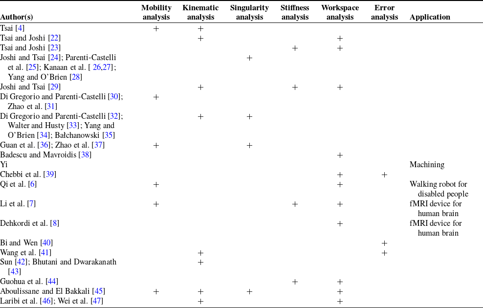
The first 3-UPU PM presented by Tsai PM generically has three DoF and is designed for pure translational motion, that is, it is a translational PM (TPM). Mobility, kinematic, singularity, dynamic, stiffness, workspace, accuracy analyses and certain applications of the Tsai 3-UPU PM were issued by several researchers. These studies are summarized in Table I. The proposed application for the Tsai PM include machining [Reference Yi5], a walking robot for disabled people [Reference Qi, Wang, Huang and Zhang6] and a functional magnetic resonance imaging (fMRI) device for examining the functioning of the human brain [Reference Li, Frisoli, Solazzi and Bergamasco7,Reference Dehkordi, Frisoli, Sotgiu and Bergamasco8].
A 3-UPU PM with a different kind of joint layout, later on called the Seoul National University(SNU) PM, was introduced at the beginning of the new millennium. When mobility analysis of the SNU PM is theoretically computed, it is seen that the PM has three translational DoF. However, when the physical model of the PM was constructed, it was observed that the PM moved even when all the actuators are locked. Even the kinematic singularity analysis of the PM has not solved this problem. Later, researchers tried to explain this phenomenon by analyzing the kinematic sensitivity of the PM [Reference Han9]. Wolf and Shoham [Reference Wolf and Shoham10], Liu et al. [Reference Liu, Lou, Li and Robot11], Walter et al. [Reference Walter, Husty and Pfurner12], Gogu [Reference Gogu13] and Qu et al. [Reference Qu, Fang and Guo14] have worked on the singularity analysis of the SNU PM. Bonev and Zlatanov [Reference Bonev and Zlatanov D15], Wolf et al. [Reference Wolf, Shoham and Park16], Zlatanov et al. [Reference Zlatanov, Bonev and Gosselin17], Li and Huang [Reference Li and Huang18], Chen et al. [Reference Chen, Zhang, Huang and Huang19] have also worked on the mobility analysis in addition to the singularity analysis. Kinematic analysis of the PM was studied by Li and Huang [Reference Li and Huang18], Wolf and Shoham [Reference Wolf and Shoham20], Walter et al. [Reference Walter, Husty and Pfurner12] and Chen et al. [Reference Chen, Zhang, Huang, Ding and Huang21].
Studies on the Tsai 3-UPU PM

Karouia and Hervé [Reference Karouia and Hervé48] designed a 3-UPU PM with a rotational platform for which necessarily the revolute (R) joint axes associated with the base and the moving platform intersect at a single point at all times of the motion of the PM. They worked on the mobility analysis of this spherical 3-UPU PM, whereas Di Gregorio [Reference Di Gregorio49] worked on the mobility, kinematic and singularity analyses of the PM. The singularity analysis of the PM was also studied by Di Gregorio [Reference Di Gregorio50] and Paganelli [Reference Paganelli51], while Chebbi et al. [Reference Chebbi, Affi and Romdhane52] and Pramanik and Ghosal [Reference Pramanik and Ghosal53] worked on kinematic and singularity analysis of the PM. Xiangzhou et al. [ Reference Xiangzhou, Hongzan and Yougao54,Reference Xiangzhou, Yougao and Hongzan55] worked on the kinematics and dynamics of the PM. Pramanik and Ghosal [Reference Pramanik and Ghosal53] offered a solar tracking system using the spherical 3-UPU PM. Ashith Shyam and Ghosal [Reference Ashith Shyam and Ghosal56] worked on path planning of this PM.
Huang and Li [Reference Huang and Li57] designed 3-UPU PMs with the first U joint axes of the base or moving platform as perpendicular to the platform planes. The first analysis shows that this new type of PM generically has 4-DoF with three translational and one rotational DoF. Kiper and Söylemez [Reference Kiper and Söylemez E58] showed that when the base and the moving platform of the PM are identical, the PM has 4-DoF and furthermore, it has a finite singularity mode with 5-DoF when the limb lengths are the same. Guo et al. [Reference Guo, Wang, Fang and Li59] investigated the position and orientation errors of the PM.
Huang et al. [Reference Huang, Li and Zuo60] presented a new type of 3-UPU TPM which is in the form of a pyramid. Yu et al. [Reference Yu, Dai, Zhao, Bi and Zong61] proposed a 3-UPU PM architecture in which the R joint axes of the U joints of the base or moving platform are positioned parallel to each other inside the platform planes. Binbin et al. [Reference Binbin, Zengming, Kai and Yu62] studied the singularities of these PMs. Miao et al. [Reference Miao, Yao and Kong63] developed a rolling mechanism using such a 3-UPU PM, where the mobility, gait and stability analyzes of the PM were done. Zhao et al. [Reference Zhao, Feng, Zhou and Jin64] proposed a new PM with SNU 3-UPU-type U joints on the base, and vertical-type U joints on the moving platform. This PM possesses one translational and two rotational DoF. Lu and Hu [Reference Lu and Hu65] presented a new type of 3-UPU PM with an asymmetrical joint set-up, that is, the three U joints on a platform do not have same type of joint configuration. Lu et al. [Reference Lu, Shi and Hu66] presented PMs with SNU-type and vertical-type U joints. Hu and Lu [Reference Hu and Lu67] presented a stiffness analysis of one of these new type of PMs. Chebbi and Parenti-Castelli [Reference Chebbi and Parenti-Castelli68] presented a study with various types of 3-UPU PMs, where the singularities of the PMs were studied and their potentials were interpreted. Wang et al. [Reference Wang and Ceccarelli69–Reference Wang, Ceccarelli and Carbone72] designed a robotic leg for 3-DoF translational motion using a 3-UPU PM. Sarabandi et al. [Reference Sarabandi, Grosch, Porta and Thomas73] worked on an asymmetric 3-UPU PM which can be reconfigured to work either as a translational or a rotational PM by flipping upside down its moving platform. Zhao et al. [Reference Zhao, Chen, Li and Huang74] presented a novel 3-UPU PM with two rotational and one translational DOF without any parasitic motion. Di Gregorio [Reference Di Gregorio75] has recently presented a comprehensive review study on 3-UPU PMs and worked out motion characteristics of the PMs with special emphasis on TPMs and spherical PMs.
This study aims to classify new 3-UPU PM architectures with typical U joint layouts, examine the instantaneous mobility characteristics of 3-UPU PMs with equilateral platforms and classify PMs with non-parasitic and parasitic motion patterns. To the best knowledge of the authors, such a classification of 3-UPU PM architectures is performed for the first time. In Section 2, PMs with the same kinematic structure as the 3-UPU PM were investigated and the properties of the PMs were introduced. In Section 3, joint layouts were created for 3-UPU PMs, and these joint layouts were mapped to each other to obtain new manipulators. When these obtained PMs were examined, it was observed that they had common limb types. In Section 4, these limb types were investigated by using screw theory. In Section 5, novel PMs are analyzed.
2. 3-UPU PM types according to joint layouts
3-UPU PMs presented in the literature were investigated and the joint layouts of the R joint axes on the platforms are examined. Based on the joint layouts of these 3-UPU PMs, new 3-UPU PM architectures are constructed.
2.1. Joint layouts of Tsai, SNU, parallel and vertical 3-UPU PMs
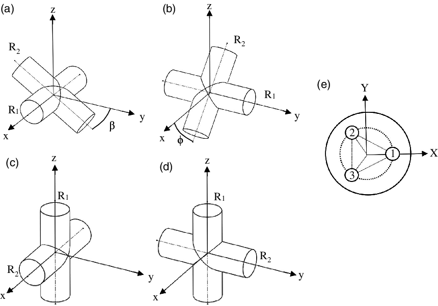
The R joint axes on the platforms of Tsai 3-UPU PM are coplanar, they form a triangle and are tangent to the circumcircle of the triangle formed by the U joint centers (Fig. 1(a)). For this reason, this kind of joint layout of the platform is denoted as UT, where T stands for tangent. The three U joint centers on the base platform define the base platform plane, whereas the three U joint centers on the moving platform define the moving platform plane. The global coordinate system (GCS) is positioned at the center of the circumcircle of the U joint centers of the base of the PM. X-axis of the GCS is oriented towards one of the U joint centers on a limb. Y-axis of the GCS lies on the base platform plane whereas the Z-axis is perpendicular to the plane. The limb which comprises the U joint center on the X-axis is numerated as limb 1 and the other two limbs are numerated as limb 2 and limb 3 by proceeding in counter-clockwise direction about the Z-axis. Three local coordinate systems (LCS) for each limb are positioned at the U joint centers of the base. The axes of LCS1 are set to be parallel to the axes of the GCS. The axis orientations of LCS2 and LCS3 differ according to the 3-UPU architecture. For the Tsai 3-UPU PM, LCS2 and LCS3 are obtained by rotating LCS1 around the Z-axis by 120° and 240°, respectively. In other words, for the Tsai 3-UPU PM, the x-axes of the LCSs are normal and the y-axes are tangent to the circumcircle. The first and second R joint axes of a U joint on the base are the first joint axis (Ri1) and second joint axis (Ri2) of each limb i (i = 1, 2, 3). A P joint is the third joint of each limb, and the next two R joint axes of the U joint on the moving platform are called the fourth joint axis (Ri4) and the fifth joint axis (Ri5) of each limb. For the Tsai 3-UPU PM, Ri1 are positioned on the y-axis of the LCSs and Ri2 rotate about the y-axis and hence lie on the xz-plane of the LCSs. Ri2 and Ri4 are parallel axes. The joint layout of the moving platform is the same as the base platform, that is, Ri5 are tangent to the circumcircle on the moving platform plane. Hence the Tsai 3-UPU PM architecture is denoted as UT-UT.
For the SNU 3-UPU PM, the R axes (Ri1 or Ri5) on a platform (base or moving) lie on the platform plane and intersect in the circumcircle center of the triangle formed by the U-joint centers and hence are normal to the circumcircle (Fig. 1(b)). This kind of joint layout of the platform is denoted as UN, where N stands for normal. Ri1 of the SNU 3-UPU PM are positioned on the x-axis of the LCSs. The base and moving platforms have the same joint layout. Ri2 and Ri4 are parallel axes. The SNU 3-UPU PM architecture is denoted as UN-UN.
When the first axes on a platform lie on the platform plane and are all parallel to the X- or Y-axis of the GCS, the joint layout of the platform is denoted as UX or UY. The LCS axes of all three limbs are parallel to the axes of the GCS axes as shown in Fig. 1(c). Depending on which R joint axes are attached to the platforms, the architecture of the PM in Fig. 1(c) may be UX-UX or UY-UY or UX-UY or UY-UX. Ri2 and Ri4 are either parallel or perpendicular to each other.
When the first R axes on a platform are perpendicular to the platform plane, the joint layout of the platform is denoted as UV. There are several possibilities for the relative positions of the Ri2 and Ri4 axes. In order to distinguish between different Ri2 and Ri4 axes configurations, an initial configuration of the PM is considered. For the PMs comprising platforms with UV type, the initial configuration of the PM, according to the orientation of the second axes the U joint (Ri2 or Ri4) may be denoted as UVT, UVN, UVX or UVY. The locations of the LCSs for Vertical 3-UPU PM is the same as the Tsai 3-UPU PM. Ri1 are positioned on the z-axes of the LCSs. For UVT, Ri2 are on the y-axes (Fig. 1(d)). For UVN, Ri2 are on the x-axes of the LCSs. For UVX and UVY, Ri2 is on either x- or y-axes of the LCSs.
Joint layouts of (a) Tsai 3-UPU PM, (b) SNU 3-UPU PM, (c) Parallel 3-UPU PM, (d) Vertical 3-UPU PM.

2.2. Sub-joint layouts for 3-UPU PMs
In general, a U-joint mounted on a platform can have ∞2 possible configurations, which depends on the orientation of the R joint axis attached to the platform. So, in general for a platform comprising three U-joints, there are ∞6 possible joint layouts. Also, the relative locations of Ri2 and Ri4 axes on each limb should be considered for a 3-UPU PM. This can be taken into account by defining the Ri2 and Ri4 axes in an initial configuration, which is specifying the angle between Ri2 and Ri4. Therefore, in general, there are ∞15 possible 3-UPU architectures. Among these abundantly many possible architectures, not all are practical. Therefore, based on the available architectures in the literature, some ground rules are established in order to narrow down the list to a reasonable finitely many possible architectures.
In the literature, it is seen that generally the distances between the U-joint centers of a platform are taken to be equivalent, that is, base and moving platforms are in equilateral triangle form. Therefore, in this study, only the 3-UPU PMs with equilateral base and moving platforms are considered. However, the base and the moving platforms need not be identical. In order to be able to perform the mobility analysis of different 3-UPU PM architectures, an initial configuration is set such that the moving platform plane is parallel to the base platform plane, the center of the moving platform is on the Z-axis of the GCS and all three limbs make a prescribed angle with the base platform plane. The relative positions of the joint axes are then defined based on this initial configuration.
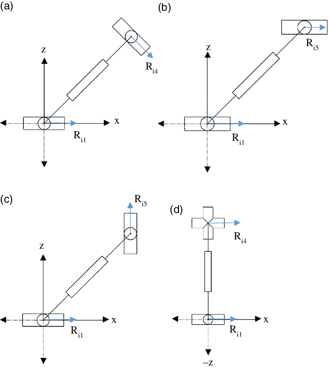
Due to the particular shape of the U joint, it is known that the position of the Ri2 and Ri4 axes can be predicted by looking at the Ri1 and Ri5 axes of the U joints. As shown in Fig. 2(a), if Ri1 axis of a U joint is along the x-axis of a LCS, Ri2 axis must move on the yz-plane. Similarly, if Ri1 axis is along the y-axis (Fig. 2(b)), Ri2 axis must move on the xz-plane. Similar arguments are valid for Ri5 and Ri4 axes of the moving platform as well.
R joint axes of a U joint when Ri1 are on (a) x-axis, (b) y-axis, (c, d) z-axis of the LCS (e) U-joint layout representation of a platform.

Ri2 and Ri4 axes have to be nonintersecting, that is, parallel or skew, because of the P joint in between them. The P joint direction cannot be in the direction of the Ri2 or Ri4 axes, otherwise a cylindrical joint is obtained. The P joint direction has to be perpendicular to Ri2 and Ri4 axes. Furthermore, it is assumed that the common normal of Ri2 and Ri4 axes pass through the two U-joint centers on limb i. With these assumptions, the orientations of Ri2 and Ri4 axes in the initial configuration of the PM are determined depending on the angle between the limbs and the platform planes. If Ri1 or Ri5 axes are perpendicular to the base or moving platform planes, that is, if Ri1 axes are on the z-axis of the corresponding LCSs, Ri2 and Ri4 have to be on the platform planes, but the relative positions of Ri2 and Ri4 axes cannot be predicted. So, in such a case, the orientation of the Ri2 and Ri4 axes in the initial configuration should be specified (Fig. 2(c) and (d)).
The case where Ri1 and Ri5 axes are neither on nor perpendicular to the platform planes is kept out of scope of this study. To sum up the previous discussions, when Ri1 or Ri5 axes are on the platform plane, the orientations of Ri2 and Ri4 axes are determined according to the angle between the limbs and the platforms in the initial configuration of the PM, while when Ri1 or Ri5 axes are perpendicular to the platform plane, the orientations of Ri2 and Ri4 axes in the initial configuration of the PM need to be specified. By this way, it is possible to provide a proper description of the PM architecture that enables to derive new U joint layouts. As seen in Fig. 2(e), the U joints are numbered in the same order as the LCSs.
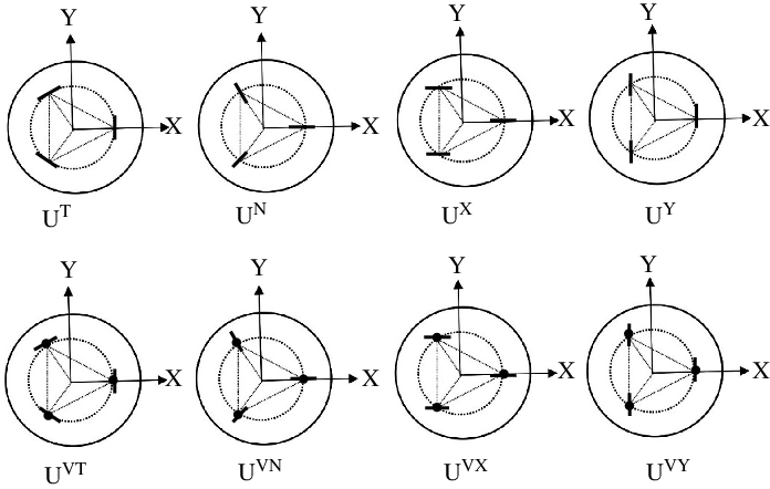
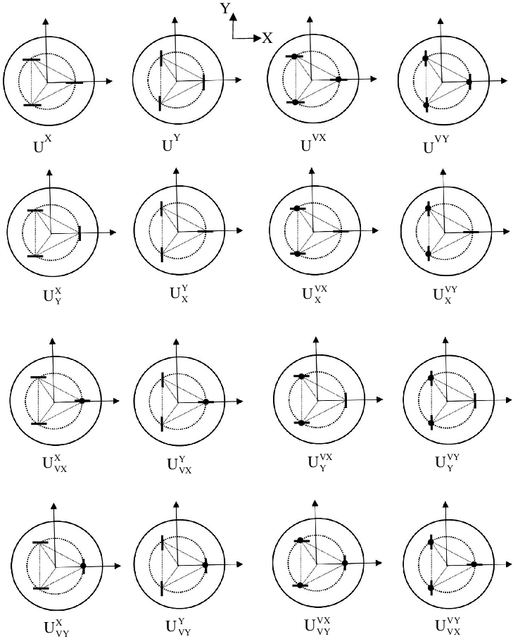
When Ri1 or Ri5 axes are on a platform plane, it is assumed that either of the following four cases occur: (1) the axes are tangent to the circle passing through the U-joint centers on a platform (UT); (2) the axes are normal to the circle passing through the U-joint centers on a platform (UN); (3) the axes are all parallel to the X-axis of the GCS (UX); (4) the axes are all parallel to the Y-axis of the GCS (UY). When Ri1 or Ri5 axes are perpendicular to a platform plane, the layout is shown with UVT, UVN, UVX or UVY, depending on whether the Ri2 or Ri4 axes are tangent, normal or parallel to X- or Y-axis, respectively. Graphical representation of all these possible U-joint layouts is illustrated in Fig. 3.
R-joint layouts of a platform.

On a platform, it is also possible to have U-joint layouts where, for example two of the Ri1 axes are tangent to the platform circle, while the remaining Ri1 axis is normal. Such new layouts are obtained by changing the type of one of the three U-joints on a platform. The changed U-joint is assumed to be on limb 1. The case, where all three U-joints are from different layouts are kept out of scope of this study. In order to represent the created subgroups, the main layout associated with the two U-joints is written as a superscript, while the U-joint to be modified is written as a subscript. For example,
 ${\rm{U}}_{\rm{N}}^{\rm{T}}$
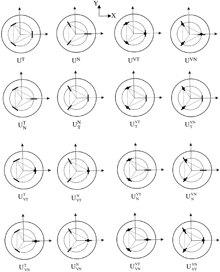
for a base platform represents a joint layout where the R11 axis is normal, while R21 and R31 are tangent to the circle passing through the U-joint centers. Different layouts for base and moving platform are not arbitrarily selected. There are two layout subgroups among which base and moving platform layouts can be matched with each other. The two main subgroups are the ones generated from UT, UN, UVT, UVN and UX, UY, UVX, UVY. Under these conditions, the sub-joint layouts are derived. For UT, UN, UVT and UVN the sub-joint layouts can be seen in Fig. 4. Sub-joint layouts for UX, UY, UVX and UVY joint layouts are shown in Fig. 5.
Sub-joint layouts for UT, UN, UVT and UVN.

Sub-joint layouts for UX, UY, UVX and UVY.

At this point, we present the whole list of assumptions for the joint layouts of the 3-UPU PMs to be classified:
-
• The base and the moving platform triangles are equilateral.
In order to define the relative joint locations, an initial configuration of the PM is set. At the initial configuration of the PM:
-
• The moving platform plane is parallel to the base platform plane.
-
• The center of the moving platform triangle is on the Z-axis of the GCS which is located at the center of the base platform triangle with Z-axis perpendicular to the base platform plane. Therefore, all three limbs make the same angle with the base platform plane.
-
• If the joint axis associated with a platform are on the platform plane, the joint axes are either tangent (denoted by T) or normal (denoted by N) to the circumcircle of the platform triangle, or else they are parallel to either X-axis (denoted by X) or Y-axis (denoted by Y) of the GCS.
-
• If the joint axis associated with a platform is perpendicular (V) to the platform plane, the consecutive joint axes are either tangent (denoted by VT) or normal (denoted by VN) to the circumcircle of the platform triangle, or else they are parallel to either X-axis (denoted by VX) or Y-axis (denoted by VY) of the GCS. As a consequence of this assumption, if any of the consecutive joint axes are not tangent to the circumcircle of the platform triangle, then the associated limb has to be perpendicular to the platform and hence the platforms are necessarily identical.
-
• A platform’s sub-joint layout is obtained by only changing the joint type associated with the first limb and keeping the joint type associated with the second and third limbs.
2.3. Novel 3-UPU PMs consisting of sub-joint layouts
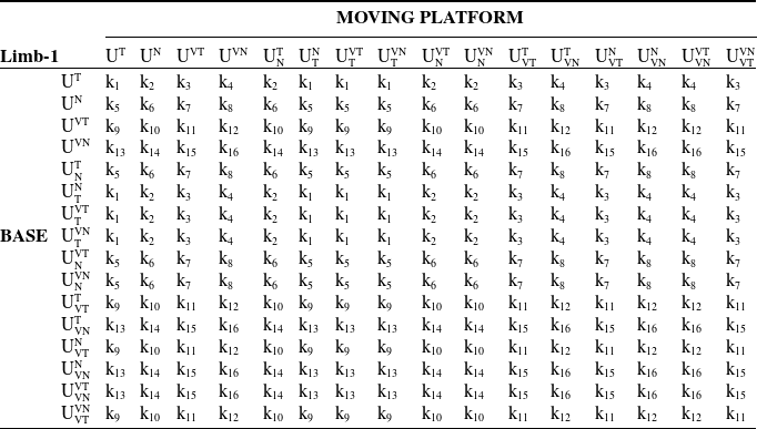
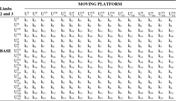
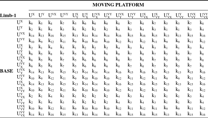
Created sub-joint layouts are matched with each other as base and moving platforms under two main groups: TNV group presented in Fig. 4 and XYV group presented in Fig. 5. Since there are 16 different sub-joint layouts in each group, a 16-by-16 table was created and 256 different PMs were derived for each group. In Section 3, the initial configurations of the PMs are taken into consideration while analyzing the mobility of the PM. To proceed with the mobility analysis, limb types are classified according to the locations of the joints on the limb in the initial configuration of the PM. Accordingly, the limbs of the TNV-type PMs are located in the xz-planes of the LCSs in the initial configuration. In XYV-type manipulators, limbs are assumed to be along the z-axes of the LCSs. Therefore, for XYV-type PMs the base and the moving platforms are assumed to be identical, because in the literature there are no XYV-type PMs with non-identical platforms and such a PM would not be a practical one. Under these assumptions, after the base and mobile platform layouts are matched to each other, it is seen that there are 16 different limb types in total (Table II). The limb types are divided into four main groups according to the locations of the Ri1 and Ri2 axes of each limb in the LCS in the initial configuration of the PM. These groups are defined such that the Ri1 or Ri2 axes are along the x-, y- or z-axis of the LCS.
The limb types with Ri1 axis parallel to the y-axis of the LCS are designated as Ry-. There are four sub-types according to the joint locations on the moving platform. As shown in Fig. 6(a), the limb type where the Ri5 axis is parallel to the y-axis of the LCS is designated as Ry–Ry. If the Ri5 axis is parallel to the x-axis of the LCS, this kind of limb is denoted as Ry–Rx (Fig. 6(b)). When Ri5 axis is parallel to the z-axis of the LCS and Ri4 axis is parallel to the y-axis of the LCS in the initial configuration of the PM, it is shown as Ry–RyRz (Fig. 6(c)), whereas if Ri4 axis is parallel to the x-axis of LCS in the initial configuration, it is shown as Ry–RxRz (Fig. 6(d)).
Symbolic equivalents of limb types

Ry-type limbs (a) Ry–Ry, (b) Ry–Rx, (c) Ry–RyRz, (d) Ry–RxRz.

The limb types with Ri1 axis parallel to the x-axis of the LCS are designated as Rx-. Since the Ri4 and Ri5 locations are the same as Ry-type limbs, the representation of second part after the P joint is similar (Fig. 7).
Rx-type limbs (a) Rx–Ry, (b) Rx–Rx, (c) Rx–RyRz, (d) Rx–RxRz.

The limb types with Ri1 axis parallel to the z-axis and Ri2 axis parallel to the y-axis of the LCS are designated as RzRy-. As shown in Fig. 8(a), the limb type with Ri5 axis parallel to the y-axis of the LCS is designated as RzRy–Ry. If Ri5 axis is parallel to the x-axis of the LCS, this kind of limb is denoted as RzRy-Rx (Fig. 8(b)). When Ri5 axis is parallel to the z-axis of the LCS and Ri4 axis is parallel to the y-axis of the LCS in the initial configuration of the PM, it is shown as RzRy–RyRz (Fig. 8(c)) whereas if Ri4 axis is parallel to the x-axis of LCS, it is shown as RzRy–RxRz (Fig. 8(d)). The limb types with Ri1 axis parallel to the z-axis and Ri2 axis parallel to the x-axis of the LCS are designated as RzRx-. Since the Ri4 and Ri5 locations are the same as RzRy-type limbs, the representation of second part after the P joint is similar (Fig. 9).
RzRy-type limbs (a) RzRy–Ry, (b) RzRy–Rx, (c) RzRy–RyRz, (d) RzRy–RxRz.

There are totally 16 limb types described in the previous subsections. For brevity, these limb types are designated with k i for i = 1, …, 16 as given in Table II.
RzRx-type limbs (a) RzRx–Ry, (b) RzRx–Rx, (c) RzRx–RyRz, (d) RzRx–RxRz.

2.4. Joint layout matching
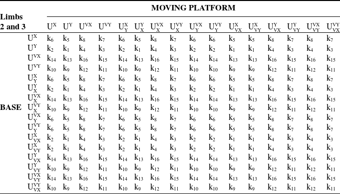
When a base and a moving platform of given joint layout are matched with each other, the limp types will be one of the 16 types given in Table II. As it is assumed that limbs 2 and 3 need to be identical while limb 1 can be different, the limbs of the TNV-type and XYV-type platforms can be classified as given in Tables III, IV, V and VI. As an example, when a
 $\mathrm{U}_{\textrm{T}}^{\textrm{VT}}$
base and a
 $\mathrm{U_N^T}$
moving platform are matched, limb 1 type is k2 (from Table II) and limbs 2 and 3 type is k9 (from Table III). By this way, it can be seen that there are 256 TNV-type PMs (each element of Tables II or III) and 256 XYV-type PMs (each element of Tables IV or V). The mobility analysis of all PMs is performed in Section 4 based on the theory presented in Section 3.
Limb types of first limbs of TNV-type PMs

Limb types of second and third limbs of TNV-type PMs

Limb types of first limbs of XYV-type PMs

Limb types of second and third limbs of XYV-type PMs

3. Joint screws of the limbs
In this section, the screw system of the limb types described in Section 2 are presented. The locations of the joint axes and the limb axes in between the universal joint centers at the terminals of the limb in the initial configuration of the PM are considered. In the initial configuration of a TNV-type PM, the limb axes are always on the xz-plane of their respective LCSs. Meanwhile, in the initial configuration of an XYV-type PM, the limb axes are along the z-axis of their respective LCSs. The angle between the limb axis and the x-axis on the xz-plane in the initial configuration of the PM is denoted by
 $\theta$
and limb length is denoted by l. For the TNV-type PMs, typical values of
 $\theta$
are used for mobility analysis: 0°, 30°, 45°, 60°, 90°. These values correspond to the cases which result in PMs with extra mobility in the literature [Reference Yang and OʼBrien28].
As seen in Fig. 10, the Ri1 joint axes of the Ry-type limbs are along the y-axis of the LCS on the base (In Figs. 10, 11, 12 and 13 ⊗ represents a screw axis along the y-axis, i.e. perpendicular to the xz-plane). For this reason, as seen in Table VII, the primary part of the first screws of the Ry-type limbs are unit vectors along the y-axis. In Table VII, c and s are abbreviations of cosine and sine, respectively. For the second screws, Ri2 joint axes of the Ry–Ry, Ry–Rx and Ry–RyRz limbs are located on the xz-plane, whereas the Ry–RxRz limb has to be along the x-axis of the LCS in the initial configuration of the PM. Hence, the primary part of the second screw of Ry–RxRz limb is the unit vector along the x-axis of the LCS. Likewise, for the third screws of Ry–RxRz limb, Ri3 joint direction has to be along the z-axis of the LCS on the base, whereas Ri3 joint directions of the rest of the limbs are on the xz-plane. The prismatic joint corresponds to infinite-pitch screws, so the secondary part of the third screw of the Ry–RxRz limb is unit vector along the z-axis, whereas it is on the xz-plane for the rest of the limbs.
Screws of Ry-type limbs (Ry–Ry, Ry–Rx, Ry–RyRz, Ry–RxRz)

For Ry–Ry limb, the primary part of the fourth screw is identical to the second screw of Ry–Ry limb. The fourth screws for Ry–Rx and Ry–RyRz limbs are identical to each other and the primary parts are the same as the first screws. For the Ry–RxRz limb the primary part of the fourth screw is unit vector along x-axis in the initial configuration of the PM. Ri5 joint axis of Ry–Ry limb is parallel to the y-axis of the LCS and the primary part of the fifth screw of Ry–Ry limb is unit vector along the y-axis in the initial configuration of the PM. Ri5 joint axis of Ry–Rx limb is parallel to the x-axis of the LCS and the primary part of the fifth screw of Ry–Rx limb is unit vector along the x-axis in the initial configuration of the PM. For the Ry–RyRz and Ry–RxRz limbs, the primary part of the fifth screws of Ry–RyRz and Ry–RxRz limbs are unit vectors along the z-axis. The screws of Ry-type limbs are given in Table VII in detail.
Screws of Ry-type limbs (a) Ry–Ry, (b) Ry–Rx, (c) Ry–RyRz, (d) Ry–RxRz.

The Ri1 joint axes of the Rx-type limbs are along the x-axis of the LCS on the base (Fig. 11). For this reason, as seen in Table VIII, the primary parts of the first screws of the Rx-type limbs are unit vectors along the x-axis. For the second screws, Ri2 joint axes of the Rx–Ry, Rx–Rx, Rx–RyRz and Rx–RxRz limbs are along the y-axis of the LCS on the base in the initial configuration of the PM, so the primary parts of the screws are unit vectors along the y-axis. The third screws of the Ry-type limbs are the same as the third screws of the Rx-type limbs. For the Rx–Ry limb, the primary part of the fourth screw is identical to the second screw of the Ry–Ry limb. The fourth screws for Rx–Rx and Rx–RyRz limbs are identical to each other and the primary parts are the same as the second screws. For the Rx–RxRz limb, the primary part of the fourth screw is unit vector along the x-axis in the initial configuration of the PM. The primary part of the fifth screw of Rx–Ry is unit vector along the y-axis in the initial configuration of the PM. The primary part of the fifth screw of the Ry–Rx limb is unit vector along the x-axis in the initial configuration of the PM. For the Rx–RyRz and Rx–RxRz, Ri5 limbs the primary part of the fifth screw is unit vector along the z-axis. The screws of Rx-type limbs are given in Table VIII in detail.
Screws of Rx-type limbs (Rx–Ry, Rx–Rx, Rx–RyRz, Rx–RxRz)

Screws of Rx-type limbs (a) Rx–Ry, (b) Rx–Rx, (c) Rx–RyRz, (d) Rx–RxRz.

The Ri1 joint axes of the RzRy-type limbs are along the z-axis of the LCS on the base (Fig. 12). For this reason, as seen in Table IX, the first screws of the RzRy-type limbs are unit vectors along the z-axis. For the second screws, Ri2 joint axes of the RzRy–Ry, RzRy–Rx, RzRy–RyRz and RzRy–RxRz limbs are along the y-axis of the LCS on the base in the initial configuration of the PM and the primary part of screws are unit vectors along the y-axis. The third screws of the RzRy-type limbs are the same as the third screws of the Rx-type limbs. For RzRy–Ry limb, the primary part of the fourth screw is identical to the second screw of Ry–Ry limb. The fourth screws for RzRy–Rx and RzRy–RyRz limbs are identical to each other and the primary parts are the same as the second screws. For the RzRy–RxRz limb, the primary part of the fourth screw is unit vector along the x-axis in the initial configuration of the PM. Ri5 joint axis of the RzRy–Ry limb is parallel to the y-axis of LCS and the primary part of the fifth screw of the RzRy–Ry limb is unit vector along the y-axis in the initial configuration of the PM. Ri5 joint axis of the RzRy–Rx limb is parallel to the x-axis of LCS and the primary part of the fifth screw of the RzRy–Rx limb is unit vector along the x-axis in the initial configuration of the PM. For the RzRy–RyRz and RzRy–RxRz limbs, the primary part of the fifth screw is unit vector along the z-axis. The screws of RzRy-type limbs are given in Table IX in detail.
The Ri1 joint axes of the RzRx-type limbs are along the z-axis of the LCS on the base (Fig. 13). For this reason, as seen in Table X, the first screws of the RzRx-type limbs are unit vectors along the z-axis. For Ri2 joint axes of the RzRx–Ry, RzRx–Rx, RzRx–RyRz and RzRx–RxRz limbs the primary part of screws are unit vectors along the x-axis. For the third screws of RzRx-type limbs, Ri3 joint axes has to be positioned along the z-axis of the LCS on the base in the initial configuration of the PM. For RzRx–Ry and RzRx–RxRz limbs, the primary part of the fourth screw is identical to the second screw of RzRx-type limbs. The fourth screws for RzRx–Rx and RzRx–RyRz limbs are identical to each other and the primary parts are unit vectors along the y-axis. The primary part of the fifth screw of RzRx–Ry is unit vector along the y-axis in the initial configuration of the PM. The fifth screw of RzRx–Rx is unit vector along the x-axis in the initial configuration of the PM. For the RzRx–RyRz and RzRx–RxRz limbs, the primary part of the fifth screw of RzRx–RyRz and RzRx–RxRz are unit vector along the z-axis. The screws of RzRx-type limbs are given in detail in Table X.
Screws of RzRy-type limbs RzRy–Ry, RzRy–Rx, RzRy–RyRz, RzRy–RxRz

Screws of RzRx-type limbs RzRx–Ry, RzRx–Rx, RzRx–RyRz, RzRx–RxRz

Screws of RzRy-type limbs (a) RzRy–Ry, (b) RzRy–Rx, (c) RzRy–RyRz, (d) RzRy–RxRz.

In Section 4, instantaneous mobility analysis of the PMs is performed using the screws of limb types. We also make use of reciprocal screws. For a screw a screw $ i = (l i , m i , n i ; p i , q i , r i )T and a reciprocal screw of $ given by $ r = (l r , m r , n r ; p r , q r , r r )T, the reciprocity condition states that l i p r + m i q r + n i r r + p i l r + q i m r + r i n r = 0. For the 3-UPU PMs, the reciprocal screw of a screw set consisting of five screws is found as
 \begin{align}\left[ {\begin{array}{c@{\quad}c@{\quad}c@{\quad}c@{\quad}c@{\quad}c} p_{1} & {{q_1}} & {{r_1}} & {{l_1}} & {{m_1}} & {{n_1}}\\[4pt]{{p_2}} & {{q_2}} & {{r_2}} & {{l_2}} & {{m_2}} & {{n_2}}\\[4pt]{{p_3}} & {{q_3}} & {{r_3}} & {{l_3}} & {{m_3}} & {{n_3}}\\[4pt]{{p_4}} & {{q_4}} & {{r_4}} & {{l_4}} & {{m_4}} & {{n_4}}\\[4pt]{{p_5}} & {{q_5}} & {{r_5}} & {{l_5}} & {{m_5}} & {{n_5}}\end{array}} \right]\left[ {\begin{array}{c}{l^{r}}\\[4pt]{{m^r}}\\[4pt]{{n^r}}\\[4pt]{{p^r}}\\[4pt]{{q^r}}\\[4pt]{{r^r}}\end{array}} \right] = \left[ {\begin{array}{c}0\\[4pt]0\\[4pt]0\\[4pt]0\\[4pt]0\\[4pt]0\end{array}} \right]\end{align}
In order to find a reciprocal screw for a limb, Dai and Jones [Reference Dai and Jones76] have developed a practical equation to solve reciprocal of a five screw system:
 \begin{align}\textit{\$}^{r} = (|\textbf{A}_{4}|, -|\textbf{A}_{5}|, |\textbf{A}_{6}|; -|\textbf{A}_{1}|, |\textbf{A}_{4}|, -|\textbf{A}_{3}|)|\textbf{A}_{4}|^{\textrm{T}}\end{align}
where A i are 5×5 submatrices obtained by removing the ith column of the 5×6 matrix in Eq. (35).
Screws of RzRx-type limbs (a) RzRx–Ry, (b) RzRx–Rx, (c) RzRx–RyRz, (d) RzRx–RxRz.

4. Instantaneous mobility analysis of 3-UPU PMs
We follow Zhao et al. [Reference Zhao, Feng, Chu and Ma77] for the mobility analyses. In order to determine the DoF of PMs, first the limbs of the PMs are examined individually in their respective LCSs. The screws of the limbs are obtained according to the LCSs. The reciprocal screws of each limb are determined (Normalization is done if necessary). The reciprocal screws created for each limb are placed in a single matrix. Finally, the set of reciprocal screws are analyzed by singular value decomposition to obtain the DoF and the motion characteristics of the PM.
 ${U_N^T} - {U_N^T}$
PM.

For a 3-UPU PM, each limb has a five-screw system. The reciprocal screws of the screws for each limb are then defined by Eq. (36). In general, three reciprocal screws are obtained for the 3-UPU PM. These screw sets are defined as
 \begin{align}{{\textit{\$}}^r} = \left[ {\begin{array}{*{20}{c}}{{\textit{\$}}_1^r}\\[5pt]{{\textit{\$}}_2^r}\\[5pt]{{\textit{\$}}_3^r}\end{array}} \right]\end{align}
Each of these screws represents a motion constraint on the platform. The set of reciprocal screws can be analyzed by singular value decomposition:
 \begin{align}\textit{\$}^{r} = \textbf{USV}|\textbf{A}_{4}|^{\rm T}\end{align}
where U is an m × m orthogonal matrix, V is an n × n orthogonal matrix and S is an m × n diagonal matrix. The rows of V T corresponding to the zero singular values of an orthonormal basis of the null space of $ r and the remaining rows of V T form an orthonormal basis of the orthogonal complement. Therefore, the dimension of the constraint space of the PM is given by d = Rank ($ r ) and the DoF of the PM is given by M = 6 – d. In V T matrix, last M rows provide the motion characteristics of the PM.
The mobility analyses were performed for all 256 TNV-type PMs and 256 XYV-type PMs. The motion patterns of all PMs are listed in Appendix A. As an illustration of the procedure, the mobility analysis of a
 $\mathrm{U_N^T}-\mathrm{U_N^T}$
PM is presented here (Fig. 14). Ri1 and Ri5 joint axes of the first limb are along the x-axis of the LCS, whereas Ri1 and Ri5 joint axes of the second and third limbs are along the y-axis of the LCSs. From Tables II and III, limb type k6 is used for the first limb, whereas limb type k1 is used for the second and third limbs. The first limb of the PM is the Rx–Rx type. The second and third limbs are of Ry–Ry type. Using Table VII, the screw set for the first limb of the manipulator is found as
 \begin{align}\textit{\$}_{11} & = (1, 0, 0;\ 0, 0, 0)\nonumber\\[3pt]\textit{\$}_{12} & = (0, 1, 0;\ 0, 0, 0)\nonumber\\[3pt]\textit{\$}_{13} & = (0, 0, 0;\ c\theta_1, 0, s\theta_1)\\[3pt]\textit{\$}_{14} & = (0, 1, 0;\ -\!l_1 s\theta_1, 0, l_1 c\theta_1)\nonumber\\[3pt]\textit{\$}_{15} & = (1, 0, 0;\ 0, l_1 s\theta_1, 0)\nonumber\end{align}
The normalized reciprocal screw for the first limb is found as
 $\textit{\$}_1^r$
= (0, 0, 0; 0, 0, s
 $\theta$
1). Using Table VI, the screw set for the second and third limbs of the manipulator are found as (for i = 2, 3)
 \begin{align}\textit{\$}_{21} & = (0, 1, 0;\ 0, 0, 0)\nonumber\\[3pt]\textit{\$}_{22} & = ( s\theta_i, 0, -c\theta_i;\ 0, 0, 0)\nonumber\\[3pt]\textit{\$}_{23} & = (0, 0, 0;\ c\theta_i, 0, s\theta_i)\\[3pt]\textit{\$}_{24} & = ( s\theta_i, 0, -c\theta_i;\ 0, l_i, 0)\nonumber\\[3pt]\textit{\$}_{25} & = (0, 1, 0;\ -l_i s\theta_i, 0, l_2 c\theta_i)\nonumber\end{align}
The normalized reciprocal screws for the second and third limbs are found as
 $\textit{\$}_2^r$
= (0, 0, 0; c
 $\theta$
2, 0, s
 $\theta$
2) and
 ${\textit{\$}}_3^r$
= (0, 0, 0; c
 $\theta$
3, 0, s
 $\theta$
3). In order to calculate the mobility of the PM, reciprocal screws calculated according to the LCS must be transformed into the GCS:
 \begin{align}\textit{\$} _{G1}^r &= \left( {{\rm{0, 0, 0;\ 0, 0, 1}}} \right)\nonumber\\[4pt]\textit{\$} _{G2}^r &= \left( {{\rm{0, 0, 0;\ }}\frac{1}{2}{\rm{c}}{\theta _2}{\rm{, }}\frac{{ - \sqrt 3 }}{2}{\rm{c}}{\theta _2}{\rm{, s}}{\theta _2}} \right)\\[4pt]\textit{\$} _{G3}^r &= \left( {{\rm{0, 0, 0;\ }}\frac{1}{2}{\rm{c}}{\theta _3}{\rm{, }}\frac{{\sqrt 3 }}{2}{\rm{c}}{\theta _3}{\rm{, s}}{\theta _3}} \right)\nonumber\end{align}
Since the all screws in Eq. (41) represent translations, the singularity analysis can be performed by looking at the determinant of the matrix composed of the secondary parts of the screws:
 \begin{align}\left| {\begin{array}{c@{\quad}c@{\quad}c}0 & 0 & 1\\[7pt]{\dfrac{1}{2}{\rm{c}}{\theta _2}} & {\dfrac{{ - \sqrt 3 }}{2}{\rm{c}}{\theta _2}} & {{\rm{s}}{\theta _2}}\\[13pt]{\dfrac{1}{2}{\rm{c}}{\theta _3}} & {\dfrac{{\sqrt 3 }}{2}{\rm{c}}{\theta _3}} & {{\rm{s}}{\theta _3}}\end{array}} \right| = \frac{{\sqrt 3 }}{2}{\rm{c}}{\theta _2}{\rm{c}}{\theta _3}\end{align}
So, the singular architectures of the PM are obtained for
 $\theta$
2 =
 $\theta$
3 = 90°. That is, if the limbs are inclined with 90° in the initial configuration of the PM, the DoF of the PM is more than 3. When the limb angles of the PM are between 0° and 90°, the DoF of the PM is 3. For this PM, the reciprocal screws already imply the motion characteristics of the PM, but nevertheless let’s check the last 3 rows of the V
T matrix obtained by singular value decomposition of the matrix:
 \begin{align}{\bf{V}}_\theta ^{\textrm{T}} = \left[ {\begin{array}{c@{\quad}c@{\quad}c@{\quad}c@{\quad}c@{\quad}c}0 & 0 & 0 & 0 & 0 & 1\\[5pt]0 & 0 & 0 & 0 & 1 & 0\\[5pt]0 & 0 & 0 & 1 & 0 & 0\end{array}} \right]\end{align}
Eq. (43) suggests that the PM is a TPM. The case where the limb angles of the PM are 90° in the initial configuration corresponds to the case of identical base and moving platforms. In this case from Eq. (41), all reciprocal screws are
 $\textit{\$} _{Gi}^r = \left( {{\rm{0, 0, 0;\ 0, 0, 1}}} \right)$
for i = 1, 2, 3, hence the PM has 5-DoF. Looking at the last five rows of the V
T matrix obtained by singular value decomposition of the matrix:
 \begin{align}{\bf{V}}_{90^\circ }^{\textrm{T}} = \left[ {\begin{array}{c@{\quad}c@{\quad}c@{\quad}c@{\quad}c@{\quad}c}0 & 1 & 0 & 0 & 0 & 0\\[5pt]1 & 0 & 0 & 0 & 0 & 0\\[5pt]0 & 0 & 0 & 0 & 0 & 1\\[5pt]0 & 0 & 0 & 0 & 1 & 0\\[5pt]0 & 0 & 0 & 1 & 0 & 0\end{array}} \right]\end{align}
So, the PM can perform all translational motions and the rotational motions except rotation about the Z-axis.
For the XYV-type PMs, the limbs are along the z-axes of the LCSs, that is,
 $\theta$
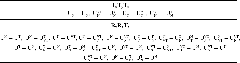
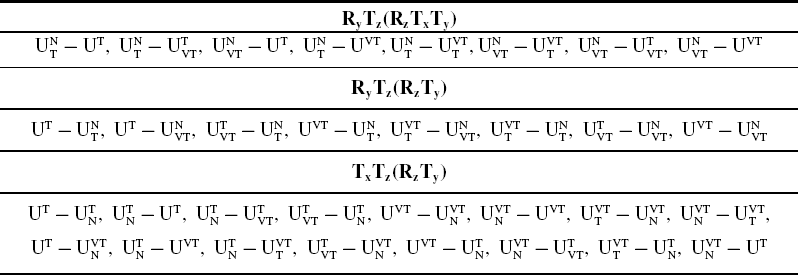
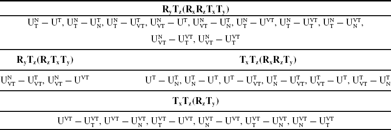
= 90°, in the initial configuration of the PM. The mobility results for all classified PMs are presented in detail in Appendix A. Tables A.I–A.X list the PMs for which non-identical platforms are permissible. In these tables, the instantaneous mobility of the PMs may change according to whether the angles of the limbs are
 $\theta$
= 0° or 0° <
 $\theta$
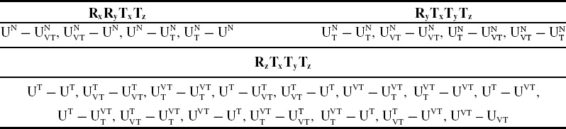
< 90° at the initial configuration of the PM. The rotation DoF of the platform about the x-, y- and z-axes are, respectively, represented by Rx, Ry, Rz, whereas the translation DoF are denoted by Tx, Ty, Tz. When a twist involves more than one nonzero element in its six coordinates, it means that the twist represents a single-DoF motion with multiple rotation and/or translation components about/along different axis, that is, there is a parasitic motion. In the tables in Appendix A, the parasitic motions are represented in parenthesis. Each pair of parenthesis represents a single-DoF twist. For example, (RzTy) means a twist with coordinates (0, 0, a; 0, b, 0) with some nonzero, but coupled elements for Rz and Ty motions. The remaining tables starting from Table A.X consist only of PMs with identical base and moving platforms, and hence
 $\theta$
= 90°.
It should be noted that the results obtained provide the instantaneous mobility of the PMs in the initial configuration. The studies do not reflect the finite mobility information. A more through kinematic analysis should be performed in order to reveal the finite mobility characteristics of a specific PM. Raw motion analysis can be performed to check the finite mobility characteristics of the PMs, for example using the Motion module of SolidWorks [Reference Gezgin78]. As an example, for the
 $\mathrm{U_N^T}-\mathrm{U_N^T}$
PM with
 $\theta$
= 0°∼90° case with non-identical base and moving platforms, the moving platform has 3-DoF with TxTyTz-type motion (Table A.VIII). When raw motion analysis is performed with random inputs for the three prismatic joints, it is seen that the orientation of the moving platform does not change. Therefore, the moving platform has three translational finite DoF, that is, the PM is a TPM. For the
 $\theta$
= 90° case, the instantaneous mobility of the PM in its initial configuration is found to be 5 with RxRyTxTyTz-type motion in Table A.XI. When the moving platform of the SolidWorks model of the PM is manually moved, it is seen that as oppose to the
 $\theta$
= 0°∼90° case, the PM is not a TPM anymore for the
 $\theta$
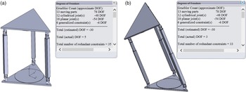
= 90° case (Fig. 15a). The raw motion analysis in SolidWorks is started from a generic configuration where the moving platform is not parallel to the base platform. At this configuration, SolidWorks evaluates the instantaneous DoF as 3 (Fig. 15b). When raw motion analysis is performed in SolidWorks Motion with random inputs for the three prismatic joints, it is seen that both of the orientation and position of the moving platform changes. Although the moving platform has three DoF, all translational and rotational motions are observed due to parasitic motions.
(a) Result of SolidWorks Motion analysis of
 $U_N^T-U_N^T$
PM when
 $\theta$
= 90° in parallel mode, (b) An arbitrary configuration for the SolidWorks Motion analysis of
 $U_N^T$
-
 $U_N^T$
PM when
 $\theta$
= 90°.

The mobility characteristics of the 3-UPU PMs existing in the literature are verified in this study. Tsai’s 3-UPU PM [Reference Tsai4] is the UT–UT PM in Table A.VIII, the SNU 3-UPU PM [Reference Han9] is the UN–UN PM in Table A.V, the parallel 3-UPU PMs [Reference Yu, Dai, Zhao, Bi and Zong61] are the UX–UX and UY–UY PMs in Table A.XVIII, the vertical 3-UPU PM [Reference Huang and Li57] are the UVT–UVT PM in Table A.VI, Zhaoʼs 3-UPU PM [Reference Zhao, Feng, Zhou and Jin64] is the UN–UVT PM in Table A.XI, Lu and Huʼs 3-UPU PM [Reference Lu and Hu65] is the
 $\mathrm{U_N^{VT}}-\mathrm{U_N^{VT}}$
PM in Table A.VIII, Hu and Luʼs 3-UPU PM [Reference Hu and Lu67] is the UVT–UN PM in Table A.X and Chebbi et al.ʼs [Reference Chebbi, Affi and Romdhane52] 3-UPU PMs are the
 $\mathrm{U_Y^X}$
–
 $\mathrm{U_X^Y}$
PM in Table A.XVIII and
 $\mathrm{U_{VT}^T}$
–
 $\mathrm{U_{VT}^T}$
PM in Table A.VIII.
Among the classified 3-UPU PMs, the 3-DoF PMs with non-parasitic motion may be considered to be valuable in applications. The DoF values in the tables in the Appendix A are instantaneous DoF values, however, if the instantaneous DoF is 3, it can be deduced that the finite DoF is also 3. The same conclusion cannot be drawn for the PMs with more than 3-DoF. Also, the instantaneous DoF being 3 is a necessary, but not sufficient condition to conclude that the finite DoF is 3.
The non-parasitic TPMs are only listed in Tables A.III and A.VIII and all these PMs are TNV-type PMs. Besides the Tsai 3-UPU PM [Reference Tsai4], there are six types of novel TPMs:
 ${\rm{U}}_{{\rm{VT}}}^{\rm{T}}-\mathrm{U_{VT}^T}$
,
 $\mathrm{U_T^{VT}}-\mathrm{U_T^{VT}}$
with
 $0^{\circ} < \theta < 90^{\circ}$
,
 ${\rm{U}}_{\rm{N}}^{\rm{T}}-\mathrm{U_N^T}$
,
 $\mathrm{U_N^{VT}}-{\rm{U}}_{\rm{N}}^{{\rm{VT}}}$
with
 $0^{\circ} \leq \theta < 90^{\circ}$
and
 $\mathrm{U_N^T}-{\rm{U}}_{\rm{N}}^{\rm{VT}}$
,
 $\mathrm{U_N^{VT}}-\mathrm{U_N^T}$
with
 $\theta = 0^{\circ}$
. Non-parasitic 3-DoF PMs with one rotational and two translation DoF are listed in Table A.XXIII with RxTyTz or RyTxTz-type motion. All such PMs are XYV-type PMs, and there are 46 many of them. Non-parasitic 3-DoF PMs with two rotational and one translational (2R1T) DoF are listed in Tables A.V, A.XI, A.XVI, A.XXIII. Among the PMs listed in these tables, the PMs with RxRzTz motion in Table A.V are different from the others, because the PMs with RxRzTz motion has both rotational and translational DoF about the z-axis. There are six such novel PMs:
 ${\rm{U}}_{{\rm{VN}}}^{\rm{T}}-\mathrm{U^{VN}}$
,
 $\mathrm{U_{VN}^T}-\mathrm{U_T^{VN}}$
,
 $\mathrm{U_{VN}^T}-\mathrm{U_N^{VN}}$
,
 $\mathrm{U_{VN}^N}-\mathrm{U^{VN}}$
,
 $\mathrm{U_{VN}^N}-\mathrm{U_T^{VN}}$
,
 $\mathrm{U_{VN}^N}-\mathrm{U_N^{VN}}$
with
 $\theta = 90^{\circ}$
. The other PMs with 2R1T motion have RxRyTz-type motion. Besides Zhaoʼs UN – UVT PM [Reference Zhao, Feng, Zhou and Jin64], there are 40 such novel PMs. Totally, 118 new 3-DoF non-parasitic 3-UPU PMs are found in this study.
5. Conclusions
In this study, different 3-UPU PM architectures are classified by considering possible joint layouts on the platforms, and the instantaneous mobility characteristics of 3-UPU PMs with equilateral platforms are investigated. Obtained 3-UPU PMs are tabulated according to their motion patterns. To the best knowledge of the authors, such a classification is performed for the first time in the literature. First, the topologies of the 3-UPU PMs available in the literature are examined and possible orientations of the U joint axes are determined. Various joint layouts are determined in accordance with the results obtained. Then, the joint layouts for the base and the moving platform are matched with each other. When these 3-UPU PM architectures are examined, it is found that they have similar limb structures. All studies are performed based on several assumptions listed in Section 2.2. The limbs are numerated and the kinematic properties of the limbs are examined using screw theory. The reciprocal screws of the limbs are derived in order to perform the instantaneous mobility analysis of PMs in their initial configurations. The results of the instantaneous mobility analysis are tabulated in order to give an insight into the future work of researchers. Also, the finite mobility analysis of one the PMs is performed using Solidworks Motion as an example.
Among the classified PMs, 118 of them are novel 3-DoF 3-UPU PMs with non-parasitic motion: 6 TPMs, 46 PMs with 1 rotational and 2 translational DoF, 6 PMs with RxRzTz and 40 PMs with RxRyTz-type motion. These non-parasitic PMs have potential use in industrial applications.
Acknowledgments
Contributions of Prof. M. İ. Can Dede and Prof. Erkin Gezgin are gratefully acknowledged.
Author Contributions
G. Kiper defined the problem; S. Boztaş came up with the assumptions and they applied the methodology together.
Financial Support
This research received no specific grant from any funding agency, commercial or not-for-profit sectors.
Competing interests
The authors declare none.
APPENDIX A
Mobility properties of TNV-type PMs with 5-DoF for
 $\theta $
= 0°

Mobility properties of TNV-type PMs with 4-DoF for
 $\theta $
= 0°

Mobility properties of TNV-type PMs with 3-DoF for
 $\theta $
= 0°

Mobility properties of TNV-type PMs with 3-DoF with one parasitic mobility for
 $\theta $
= 0°

Mobility properties of TNV-type PMs with 5-DoF for 0° <
 $\theta $
< 90°

Mobility properties of TNV-type PMs with 4-DoF for 0° <
 $\theta $
< 90°

Mobility properties of TNV-type PMs with 4-DoF with one parasitic mobility for 0° <
 $\theta $
< 90°

Mobility properties of TNV-type PMs with 3-DoF for 0° <
 $\theta $
< 90°

Mobility properties of TNV-type PMs with 3-DoF with one parasitic mobility for 0° <
 $\theta$
< 90°

Mobility properties of TNV-type PMs with 3-DoF with two parasitic mobility for 0° <
 $\theta$
< 90°

Mobility properties of TNV-type PMs with 5-DoF for
 $\theta$
= 90°

Mobility properties of TNV-type PMs with 4-DoF for
 $\theta$
= 90°

Mobility properties of TNV-type PMs with 4-DoF with one parasitic mobility for
 $\theta$
= 90°

Mobility properties of TNV-type PMs with 4-DoF with two parasitic mobility for
 $\theta$
= 90°

Mobility properties of TNV-type PMs with 3-DoF for
 $\theta$
= 90°

Mobility properties of TNV-type PMs with 3-DoF with one parasitic mobility for
 $\theta$
= 90°

Mobility properties of TNV-type PMs with 3-DoF with two parasitic mobility for
 $\theta$
= 90°

Mobility properties of XYV-type PMs with 5-DoF

Mobility properties of XYV-type PMs with 4-DoF

Mobility properties of XYV-type PMs with 4-DoF with one parasitic mobility

Mobility properties of XYV-type PMs with 4-DoF with two parasitic mobility

Mobility properties of XYV-type PMs with 4-DoF with three parasitic mobility

Mobility properties of XYV-type PMs with 3-DoF

Mobility properties of XYV-type PMs with 3-DoF with one parasitic mobility

Mobility properties of XYV-type PMs with 3-DoF with two parasitic mobility