1 Introduction
Highly viscous oils such as heavy oil (API gravity from 10 to 20, where
 $\text{API gravity}=(141.5/SG)-131.5$
and
 $SG$
is the specific gravity) and extra-heavy oil (less than 10 API gravity) become main oil reserves as the conventional crude oil has been depleted (Ismail et al.
Reference Ismail, Ismail, Zoveidavianpoor, Mohsin, Piroozian, Misnan and Sariman2015). Even though these oil reserves are estimated to be of the order of a trillion barrels in the world and constitute approximately 70 % of all oil reserves (Dusseault Reference Dusseault2001), they are hard to use because of their high viscosity in pipeline delivery. Among various drag reduction technologies, water-lubricated transport has received much attention as one of the promising tools (Ghosh et al.
Reference Ghosh, Mandal, Das and Das2009). In this arrangement, a core-annular flow is formed in which high viscosity oil is encapsulated in the pipe core region by water. Then, the water can transport the oil efficiently.
Linear stability analyses applied to a concentric phase interface between two fluids of different viscosities in a circular pipe have shown that the phase interface is always unstable when a more viscous fluid is in the annulus, whereas it can be stable (maintaining a cylindrical shape) when a more viscous fluid is in the core region and the annulus is thin enough (Joseph, Renardy & Renardy Reference Joseph, Renardy and Renardy1984; Preziosi, Chen & Joseph Reference Preziosi, Chen and Joseph1989). However, even if a more viscous fluid is located in the core region, the phase interface becomes unstable in practice and shows a wavy shape (Bai, Chen & Joseph Reference Bai, Chen and Joseph1992; Vanegas Prada & Bannwart Reference Vanegas Prada and Bannwart2001; Rodriguez & Bannwart Reference Rodriguez and Bannwart2006; Vuong Reference Vuong2009). It has been shown that the volume flow rate of the core-annular flow with a wavy phase interface is smaller than that with a cylindrically shaped phase interface (Bai et al. Reference Bai, Chen and Joseph1992), but the wavy phase interface is a necessary condition to generate a lift force on the phase interface, which prevents the phase interface from touching the wall and maintains a stable core-annular flow arrangement (Ooms et al. Reference Ooms, Segal, van der Wees, Meerhoff and Oliemans1984; Feng, Huang & Joseph Reference Feng, Huang and Joseph1995; Bai, Kelkar & Joseph Reference Bai, Kelkar and Joseph1996; Ooms, Pourquie & Beerens Reference Ooms, Pourquie and Beerens2013). Feng et al. (Reference Feng, Huang and Joseph1995) proposed that a high stagnation pressure on the windward side of the phase interface wave in the annulus generates the lift force, which was confirmed later by numerical simulations (Bai et al. Reference Bai, Kelkar and Joseph1996; Ooms et al. Reference Ooms, Pourquie and Beerens2013). Despite this important role of the phase interface wave, there are few studies about the wave characteristics in a fully developed turbulent core-annular flow (Ingen Housz et al. Reference Ingen Housz, Ooms, Henkes, Pourquie, Kidess and Radhakrishnan2017; Tripathi et al. Reference Tripathi, Tabor, Singh and Bhattacharya2017). Moreover, at a high Reynolds number, this wave shape of the phase interface is mainly caused by the turbulence in the annular flow (Hu & Joseph Reference Hu and Joseph1989; Orazzo, Coppola & De Luca Reference Orazzo, Coppola and De Luca2014). Thus, it is necessary to investigate the turbulent annular flow and its interaction with the phase interface.
Many researchers have experimentally investigated oil–water core-annular flow in a vertical pipe, and shown that core-annular flow occurs for a wide range of oil properties and flow rates and is effective in reducing the drag (Bai et al.
Reference Bai, Chen and Joseph1992; Vanegas Prada & Bannwart Reference Vanegas Prada and Bannwart2001; Rodriguez & Bannwart Reference Rodriguez and Bannwart2006; Vuong Reference Vuong2009). Bai et al. (Reference Bai, Chen and Joseph1992) provided a flow pattern map for flow in a vertical pipe of 9.5 mm diameter under superficial velocities of oil less than
 $0.9~\text{m}~\text{s}^{-1}$
, where the density and viscosity of oil used were
 $\unicode[STIX]{x1D70C}_{o}=905~\text{kg}~\text{m}^{-3}$
and
 $\unicode[STIX]{x1D707}_{o}=0.6~\text{Pa}~\text{s}$
, respectively. Here, the superficial velocities of water and oil are
 $j_{w}=q_{w}/\unicode[STIX]{x03C0}R^{2}$
and
 $j_{o}=q_{o}/\unicode[STIX]{x03C0}R^{2}$
, respectively, where
 $R$
is the pipe radius, and
 $q_{w}$
and
 $q_{o}$
are the volume flow rates of water and oil, respectively. Their data indicated that the holdup ratio (
 $s=(q_{o}/q_{w})/(V_{o}/V_{w})$
; the ratio of oil to water volume flow rates divided by the ratio of their volumes) is nearly constant,
 $s=1.39$
, where
 $V_{w}$
and
 $V_{o}$
are the volumes of water and oil, respectively. They also showed that, given an oil flow rate, there is an optimal water flow rate for minimum pressure drop, and the optimal water flow rate decreases with increasing oil flow rate. To predict the variation of the pressure drop with the superficial velocities of the oil and water, pressure drop models have been developed (Brauner Reference Brauner1991; Arney et al.
Reference Arney, Bai, Guevara, Joseph and Liu1993; Vanegas Prada & Bannwart Reference Vanegas Prada and Bannwart2001). Arney et al. (Reference Arney, Bai, Guevara, Joseph and Liu1993) obtained the friction factor of a core-annular pipe flow by combining the velocity profile of the concentric laminar core-annular flow and the Blasius friction factor. They also provided a correlation of the holdup with the fraction of water superficial velocity,
 $j_{w}/(j_{o}+j_{w})$
, by evaluating available experimental data. Here, the holdup is the volume fraction of a particular fluid (e.g. oil holdup is
 $\unicode[STIX]{x1D700}_{o}=V_{o}/V$
), where
 $V$
is the whole pipe volume. Vanegas Prada & Bannwart (Reference Vanegas Prada and Bannwart2001) conducted an experiment in a vertical pipe of 27.6 mm diameter under a superficial velocity of oil up to
 $1.75~\text{m}~\text{s}^{-1}$
(
 $\unicode[STIX]{x1D70C}_{o}=963~\text{kg}~\text{m}^{-3}$
and
 $\unicode[STIX]{x1D707}_{o}=17.6~\text{Pa}~\text{s}$
), and suggested a pressure drop model for very high viscosity oil. The model predicted the pressure drop within 25 % error, although free parameters in the model had to be adjusted.
So far, mean flow characteristics such as the flow pattern map, pressure drop and holdup have been experimentally investigated, but the details of the flow have been studied mainly by numerical simulations because of measurement difficulties. Bai et al. (Reference Bai, Kelkar and Joseph1996) conducted numerical simulations of a laminar axisymmetric core-annular flow by assuming the highly viscous core as a deformable solid, and showed that the wavelength and wave speed of the phase interface reasonably agree with those of experiments (Bai et al. Reference Bai, Chen and Joseph1992). They observed an asymmetric phase interface in the streamwise direction, i.e. steep slope in the high pressure region at the windward side and gradual slope in the low pressure region at the leeward side of the wave, respectively. Especially, the difference in the pressure across the wave crest increases with increasing Reynolds number, indicating that an inertial effect is important in the phase interface dynamics (Feng et al. Reference Feng, Huang and Joseph1995). They showed that the water flow region between the phase interface and the wall is divided into two parts; in a reference frame moving with the core velocity, one is wall-parallel flow near the wall, and the other is a recirculating flow inside a wave valley. This recirculating flow is observed to be trapped inside the wave valley and to travel downstream (Bai et al. Reference Bai, Kelkar and Joseph1996; Li & Renardy Reference Li and Renardy1999; Kouris & Tsamopoulos Reference Kouris and Tsamopoulos2002). Li & Renardy (Reference Li and Renardy1999) observed that a steady recirculating flow inside the valley becomes unsteady with increasing Reynolds number.
Huang, Christodoulou & Joseph (Reference Huang, Christodoulou and Joseph1994) studied a turbulent core-annular flow in a horizontal pipe using a
 $k{-}\unicode[STIX]{x1D700}$
turbulence model for a fixed cylindrical interface shape, and explained the effects of the eccentricity of the core on the friction factor and holdup. However, it is unrealistic to assume the phase interface shape as a cylindrical one because the wavy phase interface is a necessary condition for a stable core-annular flow. Ko et al. (Reference Ko, Choi, Bai and Joseph2002) used a shear stress transport (SST)
 $k{-}\unicode[STIX]{x1D714}$
turbulence model, and showed that the wavelength of the phase interface decreases and the stagnation pressure on the windward side increases with increasing Reynolds number. They also showed that the pressure drop of a turbulent core-annular flow is almost same as that of a single-phase water flow. Recently, time-dependent three-dimensional RANS (Reynolds-averaged Navier–Stokes) simulations have been conducted on turbulent core-annular flows in vertical and horizontal pipes (Ghosh, Das & Das Reference Ghosh, Das and Das2010; Ingen Housz et al.
Reference Ingen Housz, Ooms, Henkes, Pourquie, Kidess and Radhakrishnan2017; Shi, Gourma & Yeung Reference Shi, Gourma and Yeung2017). Ingen Housz et al. (Reference Ingen Housz, Ooms, Henkes, Pourquie, Kidess and Radhakrishnan2017) conducted both experiments and numerical simulations for a horizontal core-annular flow. They compared the pressure drop and wave characteristics from numerical simulations with those from experiments, and found a reasonably good agreement (15 % underprediction of the pressure drop). They attributed this underprediction to the turbulence model adopted. Shi et al. (Reference Shi, Gourma and Yeung2017) simulated a horizontal core-annular flow with oil having a medium viscosity ratio (
 $\unicode[STIX]{x1D707}_{o}/\unicode[STIX]{x1D707}_{w}=18.8$
), and investigated the evolution of the phase interface and the oil and water velocity distributions. The pressure drop and holdup were reasonably predicted. They also showed a few different flow patterns by considering the wettability of the pipe wall. However, results from RANS simulation change depending on the turbulence model (Shi et al.
Reference Shi, Gourma and Yeung2017), and the wave shapes obtained were smoother than those observed in experiments because the grids used in their simulations were too coarse to resolve small-scale deformation of the phase interface wave.
The phase interface between oil and water deforms in time with a broadband spectrum and the flow dynamics strongly depends on the shape of the phase interface. However, the spatio-temporal characteristics of the wave dynamics and its interaction with the flow have not been fully investigated by previous experimental and numerical studies, and thus they need to be studied by more accurate, unsteady numerical simulations. In the present study, we conduct direct numerical simulations of turbulent core-annular flow in a vertical pipe for five different oil holdups by keeping a constant mean pressure gradient in the pipe. No turbulence model is used and small-scale turbulence is resolved in the present simulation. We use a level-set method to track the oil–water interface in space and time. Details of numerical methods and flow conditions are introduced in § 2. Section 3.1 discusses the flow characteristics of high viscosity oil in the core region and water in the annular region, respectively, together with the variation of flow statistics with the oil holdups. The power spectral density and convection velocity of the phase interface are given in § 3.2, followed by a predictive model for the oil holdup in § 3.3. Finally, conclusions are given in § 4.
2 Computational details
To track the phase interface between two immiscible fluids, high viscosity oil and water, a level-set method is adopted (Herrmann Reference Herrmann2008; Kim & Moin Reference Kim and Moin2011):
 $$\begin{eqnarray}\displaystyle & \displaystyle {\displaystyle \frac{\unicode[STIX]{x2202}\unicode[STIX]{x1D719}}{\unicode[STIX]{x2202}t}}+u_{j}{\displaystyle \frac{\unicode[STIX]{x2202}\unicode[STIX]{x1D719}}{\unicode[STIX]{x2202}x_{j}}}=0, & \displaystyle\end{eqnarray}$$
where
 $x_{j}$
are the cylindrical coordinates,
 $u_{j}$
are the corresponding velocity components and
 $\unicode[STIX]{x1D719}$
is the level-set function which is a signed-distance function from the phase interface having positive values in water, negative ones in oil and is zero at the phase interface. Equation (2.1) is solved at grids near the phase interface using a third-order total variation diminishing (TVD) Runge–Kutta method in time (Gottlieb & Shu Reference Gottlieb and Shu1998) and a fifth-order weighted essentially non-oscillatory (WENO) scheme in space in conjunction with a local Lax–Friedrichs entropy correction (Jiang & Peng Reference Jiang and Peng2000). Due to unsteady fluid velocity, the level-set function updated by (2.1) does not preserve the signed-distance property,
 $|\unicode[STIX]{x1D735}\unicode[STIX]{x1D719}|=1$
. We use a partial differential equation based re-initialization method (Sussman, Smereka & Osher Reference Sussman, Smereka and Osher1994; Peng et al.
Reference Peng, Merriman, Osher, Zhao and Kang1999) to maintain this property:
 $$\begin{eqnarray}\displaystyle & \displaystyle {\displaystyle \frac{\unicode[STIX]{x2202}\unicode[STIX]{x1D719}}{\unicode[STIX]{x2202}\unicode[STIX]{x1D70F}_{r}}}+{\displaystyle \frac{\unicode[STIX]{x1D719}}{\sqrt{\unicode[STIX]{x1D719}^{2}+|\unicode[STIX]{x1D735}\unicode[STIX]{x1D719}|^{2}\unicode[STIX]{x1D6E5}_{G}^{2}}}}(|\unicode[STIX]{x1D735}\unicode[STIX]{x1D719}|-1)=0, & \displaystyle\end{eqnarray}$$
where
 $\unicode[STIX]{x1D70F}_{r}$
is the pseudo time for the re-initialization iteration and
 $\unicode[STIX]{x1D6E5}_{G}$
is the grid spacing. Equation (2.2) is iteratively solved using the third-order TVD Runge–Kutta method in time and the fifth-order WENO scheme with a Godunov flux scheme in space. Then, the converged level-set function becomes the signed-distance function. For incompressible flow, the volume of each fluid should be conserved, but the level-set method does not preserve this property due to an unresolved sub-grid-scale deformation. To compensate the volume loss, we relocate the phase interface to keep the total oil volume as the one given at the initial time step (Son Reference Son2001; Zhang, Zou & Greaves Reference Zhang, Zou and Greaves2010):
 $$\begin{eqnarray}\displaystyle & \displaystyle {\displaystyle \frac{\unicode[STIX]{x2202}\unicode[STIX]{x1D719}}{\unicode[STIX]{x2202}\unicode[STIX]{x1D70F}_{v}}}={\displaystyle \frac{\unicode[STIX]{x1D719}}{\sqrt{\unicode[STIX]{x1D719}^{2}+|\unicode[STIX]{x1D735}\unicode[STIX]{x1D719}|^{2}\unicode[STIX]{x1D6E5}_{G}^{2}}}}{\displaystyle \frac{V_{o}(t)-V_{o}(t=0)}{V_{o}(t=0)}}, & \displaystyle\end{eqnarray}$$
where
 $\unicode[STIX]{x1D70F}_{v}$
is the pseudo time for the volume correction iteration, and
 $V_{o}(t)$
is the volume of oil defined as
 $$\begin{eqnarray}\displaystyle & \displaystyle V_{o}(t)=\int (1-\unicode[STIX]{x1D713})\,\text{d}V. & \displaystyle\end{eqnarray}$$
Here,
 $\unicode[STIX]{x1D713}$
is the water volume fraction in a control volume calculated from the linearization of the level-set function (van der Pijl et al.
Reference van der Pijl, Segal, Vuik and Wesseling2005; Herrmann Reference Herrmann2008), and thus
 $\unicode[STIX]{x1D713}=0$
or 1 for the cells containing oil or water only, respectively, and
 $0<\unicode[STIX]{x1D713}<1$
for the cells containing the phase interface. Equation (2.3) is iteratively solved until the volume difference,
 $(V_{o}(t=0)-V_{o}(t))/V_{o}(t=0)$
, is smaller than a tolerance level of
 $10^{-5}$
. We confirm that maximum differences in the volume fraction
 $\unicode[STIX]{x1D713}$
before and after the volume correction are only
 $O(10^{-5})$
, so the position of the phase interface little changes during this procedure.
The governing equations for unsteady incompressible two-phase flow are
 $$\begin{eqnarray}\displaystyle & \displaystyle {\displaystyle \frac{\unicode[STIX]{x2202}(\unicode[STIX]{x1D70C}u_{i})}{\unicode[STIX]{x2202}t}}+{\displaystyle \frac{\unicode[STIX]{x2202}(\unicode[STIX]{x1D70C}u_{i}u_{j})}{\unicode[STIX]{x2202}x_{j}}}=-{\displaystyle \frac{\text{d}P}{\text{d}x}}\unicode[STIX]{x1D6FF}_{i1}-{\displaystyle \frac{\unicode[STIX]{x2202}p}{\unicode[STIX]{x2202}x_{i}}}+{\displaystyle \frac{\unicode[STIX]{x2202}}{\unicode[STIX]{x2202}x_{j}}}\left[\unicode[STIX]{x1D707}\left({\displaystyle \frac{\unicode[STIX]{x2202}u_{i}}{\unicode[STIX]{x2202}x_{j}}}+{\displaystyle \frac{\unicode[STIX]{x2202}u_{j}}{\unicode[STIX]{x2202}x_{i}}}\right)\right]-\unicode[STIX]{x1D70C}g\unicode[STIX]{x1D6FF}_{i1}+\unicode[STIX]{x1D70E}\unicode[STIX]{x1D705}\unicode[STIX]{x1D6FF}n_{i},\qquad & \displaystyle\end{eqnarray}$$
 $$\begin{eqnarray}\displaystyle & \displaystyle {\displaystyle \frac{\unicode[STIX]{x2202}u_{i}}{\unicode[STIX]{x2202}x_{i}}}=0, & \displaystyle\end{eqnarray}$$
where
 $-\text{d}P/\text{d}x$
is the mean pressure gradient,
 $p$
is the pressure fluctuations,
 $g$
is the gravitational acceleration,
 $\unicode[STIX]{x1D70E}$
is the surface tension coefficient,
 $\unicode[STIX]{x1D705}$
is the curvature,
 $n_{i}$
is the surface-normal vector on the phase interface,
 $\unicode[STIX]{x1D6FF}_{i1}$
is the Kronecker delta (1 for the streamwise (or axial) direction (
 $i=1$
) and 0 otherwise) and
 $\unicode[STIX]{x1D6FF}$
is the delta function (non-zero value at the phase interface and zero otherwise). The density and viscosity are constants for each fluid, but change continuously near the phase interface like
 $$\begin{eqnarray}\displaystyle & \displaystyle \unicode[STIX]{x1D70C}=\unicode[STIX]{x1D70C}_{o}+(\unicode[STIX]{x1D70C}_{w}-\unicode[STIX]{x1D70C}_{o})\unicode[STIX]{x1D713}, & \displaystyle\end{eqnarray}$$
 $$\begin{eqnarray}\displaystyle & \displaystyle \unicode[STIX]{x1D707}=\unicode[STIX]{x1D707}_{o}+(\unicode[STIX]{x1D707}_{w}-\unicode[STIX]{x1D707}_{o})\unicode[STIX]{x1D713}, & \displaystyle\end{eqnarray}$$
where the subscripts
 $w$
and
 $o$
denote water and oil, respectively. The continuous viscosity distribution allows the viscous term in (2.5) to be discretized using a second-order central difference scheme (Kang, Fedkiw & Liu Reference Kang, Fedkiw and Liu2000). To solve (2.5) and (2.6), the density at the next time step should be known a priori. Thus, a provisional density (
 $\hat{\unicode[STIX]{x1D70C}}$
) is obtained from the continuity equation,
 $$\begin{eqnarray}\displaystyle & \displaystyle {\displaystyle \frac{\unicode[STIX]{x2202}\unicode[STIX]{x1D70C}}{\unicode[STIX]{x2202}t}}+{\displaystyle \frac{\unicode[STIX]{x2202}(\unicode[STIX]{x1D70C}u_{j})}{\unicode[STIX]{x2202}x_{j}}}=0, & \displaystyle\end{eqnarray}$$
using an upwind-type mass-flux scheme (Kim & Moin Reference Kim and Moin2011; Raessi & Pitsch Reference Raessi and Pitsch2012) as follows:
 $\hat{\unicode[STIX]{x1D70C}}=\unicode[STIX]{x1D70C}^{n}-(\unicode[STIX]{x0394}t/\unicode[STIX]{x0394}V)\sum _{i}\unicode[STIX]{x0394}D_{i}$
, where
 $\unicode[STIX]{x0394}D_{i}=[\unicode[STIX]{x1D70C}_{o}+(\unicode[STIX]{x1D70C}_{w}-\unicode[STIX]{x1D70C}_{o})\unicode[STIX]{x1D713}_{\unicode[STIX]{x1D6E4}_{i}}](u_{i}^{n}n_{i}^{\ast })\unicode[STIX]{x0394}A_{i}$
,
 $\unicode[STIX]{x1D713}_{\unicode[STIX]{x1D6E4}_{i}}$
is the water volume fraction of
 $\unicode[STIX]{x1D6E4}_{i}(=|u_{i}^{n}n_{i}^{\ast }|\unicode[STIX]{x0394}A_{i}\unicode[STIX]{x0394}t)$
,
 $\unicode[STIX]{x0394}V$
is the grid cell volume,
 $n_{i}^{\ast }$
is the unit normal vector to the cell surface of
 $\unicode[STIX]{x0394}A_{i}$
and
 $\unicode[STIX]{x0394}t$
is the computational time step size, respectively.
Equations (2.5) and (2.6) are solved using a four-step fractional step method (Choi & Moin Reference Choi and Moin1994):
 $$\begin{eqnarray}\displaystyle & & \displaystyle \hspace{-12.0pt}\displaystyle {\displaystyle \frac{\hat{\unicode[STIX]{x1D70C}}\hat{u} _{i}-\unicode[STIX]{x1D70C}^{n}u_{i}^{n}}{\unicode[STIX]{x0394}t}}+{\displaystyle \frac{1}{2}}{\displaystyle \frac{\unicode[STIX]{x2202}}{\unicode[STIX]{x2202}x_{j}}}(\hat{\unicode[STIX]{x1D70C}}\hat{u} _{i}\hat{u} _{j}+\unicode[STIX]{x1D70C}^{n}u_{i}^{n}u_{j}^{n})=-{\displaystyle \frac{\text{d}P}{\text{d}x}}\unicode[STIX]{x1D6FF}_{i1}-{\displaystyle \frac{\unicode[STIX]{x2202}p^{n}}{\unicode[STIX]{x2202}x_{i}}}\nonumber\\ \displaystyle & & \displaystyle \displaystyle \quad +\,{\displaystyle \frac{1}{2}}{\displaystyle \frac{\unicode[STIX]{x2202}}{\unicode[STIX]{x2202}x_{j}}}\left[\hat{\unicode[STIX]{x1D707}}\left({\displaystyle \frac{\unicode[STIX]{x2202}\hat{u} _{i}}{\unicode[STIX]{x2202}x_{j}}}+{\displaystyle \frac{\unicode[STIX]{x2202}\hat{u} _{j}}{\unicode[STIX]{x2202}x_{i}}}\right)+\unicode[STIX]{x1D707}^{n}\left({\displaystyle \frac{\unicode[STIX]{x2202}u_{i}^{n}}{\unicode[STIX]{x2202}x_{j}}}+{\displaystyle \frac{\unicode[STIX]{x2202}u_{j}^{n}}{\unicode[STIX]{x2202}x_{i}}}\right)\right]-{\displaystyle \frac{1}{2}}(\hat{\unicode[STIX]{x1D70C}}+\unicode[STIX]{x1D70C}^{n})g\unicode[STIX]{x1D6FF}_{i1}+\unicode[STIX]{x1D70E}\unicode[STIX]{x1D705}^{n}\unicode[STIX]{x1D6FF}^{n}n_{i}^{n},\nonumber\\ \displaystyle & & \displaystyle\end{eqnarray}$$
 $$\begin{eqnarray}\displaystyle & \displaystyle {\displaystyle \frac{\hat{\unicode[STIX]{x1D70C}}u_{i}^{\ast }-\hat{\unicode[STIX]{x1D70C}}\hat{u} _{i}}{\unicode[STIX]{x0394}t}}={\displaystyle \frac{\unicode[STIX]{x2202}p^{n}}{\unicode[STIX]{x2202}x_{i}}}, & \displaystyle\end{eqnarray}$$
 $$\begin{eqnarray}\displaystyle & \displaystyle {\displaystyle \frac{\unicode[STIX]{x2202}}{\unicode[STIX]{x2202}x_{i}}}\left({\displaystyle \frac{1}{\hat{\unicode[STIX]{x1D70C}}}}{\displaystyle \frac{\unicode[STIX]{x2202}p^{n+1}}{\unicode[STIX]{x2202}x_{i}}}\right)={\displaystyle \frac{1}{\unicode[STIX]{x0394}t}}{\displaystyle \frac{\unicode[STIX]{x2202}u_{i}^{\ast }}{\unicode[STIX]{x2202}x_{i}}}, & \displaystyle\end{eqnarray}$$
 $$\begin{eqnarray}\displaystyle & \displaystyle {\displaystyle \frac{\hat{\unicode[STIX]{x1D70C}}u_{i}^{n+1}-\hat{\unicode[STIX]{x1D70C}}u_{i}^{\ast }}{\unicode[STIX]{x0394}t}}=-{\displaystyle \frac{\unicode[STIX]{x2202}p^{n+1}}{\unicode[STIX]{x2202}x_{i}}}, & \displaystyle\end{eqnarray}$$
where
 $\hat{\unicode[STIX]{x1D707}}$
is the viscosity calculated from (2.8) with
 $\unicode[STIX]{x1D713}$
obtained from
 $\unicode[STIX]{x1D70C}=\hat{\unicode[STIX]{x1D70C}}$
in (2.7), and the superscript
 $n$
is the time step index. As the Navier–Stokes equations and the level-set method are decoupled, the time lag between the pressure and surface tension forces at the phase interface causes a force imbalance at the phase interface. The balance is achieved by treating the surface tension term explicitly as a source term in (2.10) with a continuum surface force approach (Brackbill, Kothe & Zemach Reference Brackbill, Kothe and Zemach1992), and obtaining the pressure to balance the surface tension term (Francois et al.
Reference Francois, Cummins, Dendy, Kothe, Sicilian and Williams2006; Herrmann Reference Herrmann2008). The second-order central difference scheme is used for all the spatial derivative terms except the convection term near the phase interface where the same upwind-type mass-flux scheme used to solve (2.9) is applied for the consistent mass and momentum transport (Kim & Moin Reference Kim and Moin2011; Raessi & Pitsch Reference Raessi and Pitsch2012). A Newton iteration method with an approximate factorization (Choi, Moin & Kim Reference Choi, Moin and Kim1992) and an Aitken-type accelerator (Irons & Tuck Reference Irons and Tuck1969) is adopted to solve the resulting system matrix. An iterative constant-coefficient Poisson solver (Kim & Moin Reference Kim and Moin2011) using a fast Fourier transform is applied to solve the variable-coefficient pressure Poisson equation (2.12) together with (2.13):
 $$\begin{eqnarray}\displaystyle & \displaystyle {\displaystyle \frac{\unicode[STIX]{x2202}}{\unicode[STIX]{x2202}x_{i}}}{\displaystyle \frac{\unicode[STIX]{x2202}p^{n+1,m+1}}{\unicode[STIX]{x2202}x_{i}}}={\displaystyle \frac{\unicode[STIX]{x1D70C}_{o}}{\unicode[STIX]{x0394}t}}{\displaystyle \frac{\unicode[STIX]{x2202}u_{i}^{m}}{\unicode[STIX]{x2202}x_{i}}}, & \displaystyle\end{eqnarray}$$
 $$\begin{eqnarray}\displaystyle & \displaystyle u_{i}^{m+1}=u_{i}^{m}-{\displaystyle \frac{\unicode[STIX]{x0394}t}{\hat{\unicode[STIX]{x1D70C}}}}{\displaystyle \frac{\unicode[STIX]{x2202}p^{n+1,m+1}}{\unicode[STIX]{x2202}x_{i}}}, & \displaystyle\end{eqnarray}$$
where the superscript
 $m$
is the iteration index. The convergence using this method is much faster for a density ratio close to unity like the present one (
 $\unicode[STIX]{x1D70C}_{w}/\unicode[STIX]{x1D70C}_{o}=1.036$
) than that using a variable-coefficient solver such as conjugate-gradient-type methods. Equations (2.14) and (2.15) are iteratively solved with
 $u_{i}^{m=0}=u_{i}^{\ast }$
, and the final velocity and pressure are
 $u_{i}^{n+1}=u_{i}^{m+1}$
and
 $p^{n+1}=\sum _{k=1}^{m+1}p^{n+1,k}$
. Approximately six iterations is enough to satisfy the convergence criterion of
 $|\unicode[STIX]{x2202}u_{i}^{m+1}/\unicode[STIX]{x2202}x_{i}|_{max}<10^{-5}$
, and it consumes approximately 10 % of the whole computational time. Once the velocity is obtained from (2.10) to (2.13), the phase interface is updated by solving the level-set equation (2.1). The present numerical method is globally second-order accurate and its details are available in Herrmann (Reference Herrmann2008) and Kim & Moin (Reference Kim and Moin2011). The density and viscosity of oil used for present simulations are
 $\unicode[STIX]{x1D70C}_{o}=963~\text{kg}~\text{m}^{-3}$
and
 $\unicode[STIX]{x1D707}_{o}=17.6~\text{Pa}~\text{s}$
(Vanegas Prada & Bannwart Reference Vanegas Prada and Bannwart2001) and those of water are
 $\unicode[STIX]{x1D70C}_{w}=998~\text{kg}~\text{m}^{-3}$
and
 $\unicode[STIX]{x1D707}_{w}=0.001~\text{Pa}~\text{s}$
, respectively. Note that the viscosity of oil is 17 600 times that of water. Therefore,
 $\unicode[STIX]{x1D707}\simeq \unicode[STIX]{x1D707}_{o}$
unless
 $\unicode[STIX]{x1D713}$
(water volume fraction)
 ${\approx}1$
(see (2.8)), implying that the fluid in a cell containing only a small amount of oil flows like a core. Thus, to visualize the water flow near the phase interface, we identify the instantaneous phase interface with
 $\unicode[STIX]{x1D713}=0.95$
. We assume that oil under consideration is Newtonian, which was also reported in Vanegas Prada (Reference Vanegas Prada1999). The surface tension coefficient is
 $\unicode[STIX]{x1D70E}=0.03~\text{N}~\text{m}^{-1}$
(Bannwart Reference Bannwart2001).
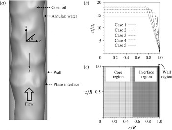
(a) Schematic diagram of the core-annular flow in a vertical pipe; (b) initial velocity profiles; (c) grid distribution for case 3 (
 $\unicode[STIX]{x1D700}_{o}=0.71$
, see table 1). In (b), the velocity profiles abruptly change across the phase interfaces.

Figure 1(a) shows the schematic diagram of the core-annular flow in a vertical pipe. The momentum balance applied to the pipe (figure 1 a) reads
 $$\begin{eqnarray}\displaystyle & \displaystyle -{\displaystyle \frac{\text{d}P}{\text{d}x}}={\displaystyle \frac{2\overline{\unicode[STIX]{x1D70F}}_{w}}{R}}+{\displaystyle \frac{1}{V}}\int \unicode[STIX]{x1D70C}g\,\text{d}V, & \displaystyle\end{eqnarray}$$
where
 $-\text{d}P/\text{d}x$
is the mean pressure gradient,
 $\int \unicode[STIX]{x1D70C}g\,\text{d}V$
is the gravitational force and
 $\overline{\unicode[STIX]{x1D70F}}_{w}$
is the mean wall shear stress on the pipe wall. When (2.16) is normalized by the friction velocity (
 $u_{\unicode[STIX]{x1D70F}}=\sqrt{\overline{\unicode[STIX]{x1D70F}}_{w}/\unicode[STIX]{x1D70C}_{w}}$
) and pipe radius (
 $R$
), it becomes
 $$\begin{eqnarray}\displaystyle & \displaystyle -{\displaystyle \frac{\text{d}P/\text{d}x}{\unicode[STIX]{x1D70C}_{w}u_{\unicode[STIX]{x1D70F}}^{2}/R}}=2+{\displaystyle \frac{\displaystyle \int \unicode[STIX]{x1D70C}g\,\text{d}V/V}{\unicode[STIX]{x1D70C}_{w}u_{\unicode[STIX]{x1D70F}}^{2}/R}}. & \displaystyle\end{eqnarray}$$
In the present study, the friction Reynolds number is fixed at
 $Re_{\unicode[STIX]{x1D70F}}=u_{\unicode[STIX]{x1D70F}}R/\unicode[STIX]{x1D708}_{w}=720$
, where
 $\unicode[STIX]{x1D708}_{w}$
is the kinematic viscosity of water. This Reynolds number is chosen from one of the measured experimental data (
 $2\overline{\unicode[STIX]{x1D70F}}_{w}/R=400~\text{Pa}~\text{m}^{-1}$
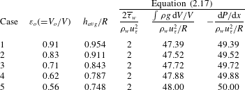
) in Vanegas Prada & Bannwart (Reference Vanegas Prada and Bannwart2001). Note that in this experiment the superficial velocities of oil and water were fixed and the mean pressure gradient to drive oil–water flow was measured. However, with a periodic boundary condition in the streamwise direction (unlike with the inflow–outflow boundary condition), one cannot prescribe both volumes and superficial velocities of two fluids under a constant mean pressure gradient (Kouris & Tsamopoulos Reference Kouris and Tsamopoulos2001). Thus, we fix the oil holdup (
 $\unicode[STIX]{x1D700}_{o}=V_{o}/V$
) and mean pressure gradient (see table 1), and obtain the superficial velocities of oil and water (varying in time). In this way, the mean radial locations of the phase interface are pre-determined as
 $h_{avg}/R=\unicode[STIX]{x1D700}_{o}^{1/2}$
(table 1); within the present range of
 $\unicode[STIX]{x1D700}_{o}$
, the phase interface neither touches the pipe wall nor breaks during simulation. Note also that the gravitational force consumes most of the mean pressure gradient but contributes little to the dynamics of fluid flow.
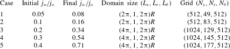
Cases considered: oil holdup, mean radial location of the phase interface and mean pressure gradient.

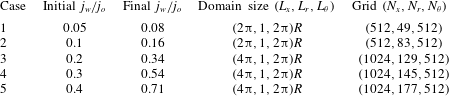
Flow conditions, computational domain sizes and number of grid points.
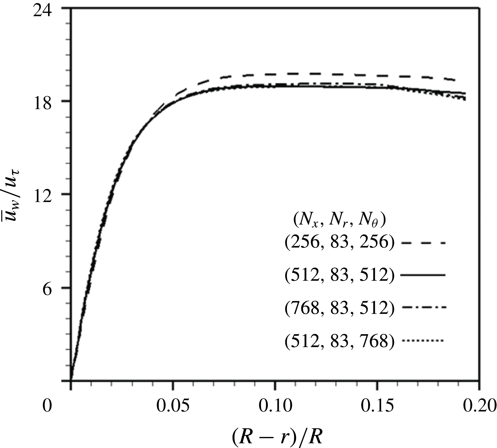
Resolution study for
 $\unicode[STIX]{x1D700}_{o}=0.83$
: profiles of the mean streamwise velocity of water.

All variables are non-dimensionalized by the pipe radius and the friction velocity unless otherwise stated. At
 $t=0$
, we start with five different volume flow rate ratios (
 $q_{w}/q_{o}$
, or superficial velocity ratios
 $j_{w}/j_{o}$
) by providing the analytic solution of laminar core-annular flow having cylindrically shaped phase interfaces (Bai et al.
Reference Bai, Chen and Joseph1992, see figure 1b), and computations are carried out for about
 $20R/u_{\unicode[STIX]{x1D70F}}$
. The superficial velocity ratio
 $j_{w}/j_{o}$
changes in time and converges to a value different from that provided at
 $t=0$
, because the velocities in water and oil vary in time under a given mean pressure gradient and oil holdup. We also numerically confirm that, with the present problem setting, an initial velocity profile different from that in figure 1(b) does not change the final superficial velocities of oil and water. Table 2 shows the computational domain sizes and number of grid points for five initial superficial velocity ratios, together with the changes in the superficial velocity ratios after the simulation. The streamwise domain sizes are
 $2\unicode[STIX]{x03C0}R$
and
 $4\unicode[STIX]{x03C0}R$
for low and high superficial velocity ratios, respectively, because the most energetic streamwise wavelength increases with increasing superficial velocity ratio (Bai Reference Bai1995; Rodriguez & Bannwart Reference Rodriguez and Bannwart2006). Periodic boundary conditions are applied in the streamwise (
 $x$
) and azimuthal (
 $\unicode[STIX]{x1D703}$
) directions where uniform grids are used, and the no-slip boundary condition is used at the wall. Figure 1(c) shows the typical grid distribution in the radial (
 $r$
) direction, where dense grids are located in the wall and interface regions but coarse grids are located in the core region in which laminar flow is expected due to the high viscosity of oil. Grid resolutions in wall units are
 $\unicode[STIX]{x0394}x^{+}=\unicode[STIX]{x0394}xu_{\unicode[STIX]{x1D70F}}/\unicode[STIX]{x1D708}_{w}\approx 8.8$
,
 $r_{min}^{+}\approx 0.2{-}0.4$
and
 $R\unicode[STIX]{x0394}\unicode[STIX]{x1D703}^{+}\approx 8.8$
. An instantaneous flow field is interpolated onto
 $1.5$
times refined grids in the azimuthal direction for
 $\unicode[STIX]{x1D700}_{o}=0.83$
(case 2), and the simulation is carried out for
 $3R/u_{\unicode[STIX]{x1D70F}}$
, resulting in negligible changes in the final total bulk velocity (
 $j_{w}+j_{o}$
) and superficial velocity ratio (
 $j_{w}/j_{o}$
). For
 $1.5$
times refined grids in the streamwise direction, the changes are less than 2 %. The profiles of the mean streamwise velocity of water (see (3.2)) in figure 2 also indicate that the present resolution is adequate. The size of computational time step is restricted mainly by the surface tension term as (Brackbill et al.
Reference Brackbill, Kothe and Zemach1992)
 $$\begin{eqnarray}\displaystyle & \displaystyle \unicode[STIX]{x0394}t\leqslant \sqrt{{\displaystyle \frac{(\unicode[STIX]{x1D70C}_{o}+\unicode[STIX]{x1D70C}_{w})\unicode[STIX]{x1D6E5}_{G}^{3}}{4\unicode[STIX]{x03C0}\unicode[STIX]{x1D70E}}}}, & \displaystyle\end{eqnarray}$$
and the corresponding CFL (Courant–Friedrichs–Lewy) number for the present problems is
 $0.05{-}0.15$
. The velocity components in (
 $x,r,\unicode[STIX]{x1D703}$
) are denoted as (
 $u,v,w$
) or (
 $u_{x},u_{r},u_{\unicode[STIX]{x1D703}}$
).
3 Results and discussion
3.1 Flow characteristics
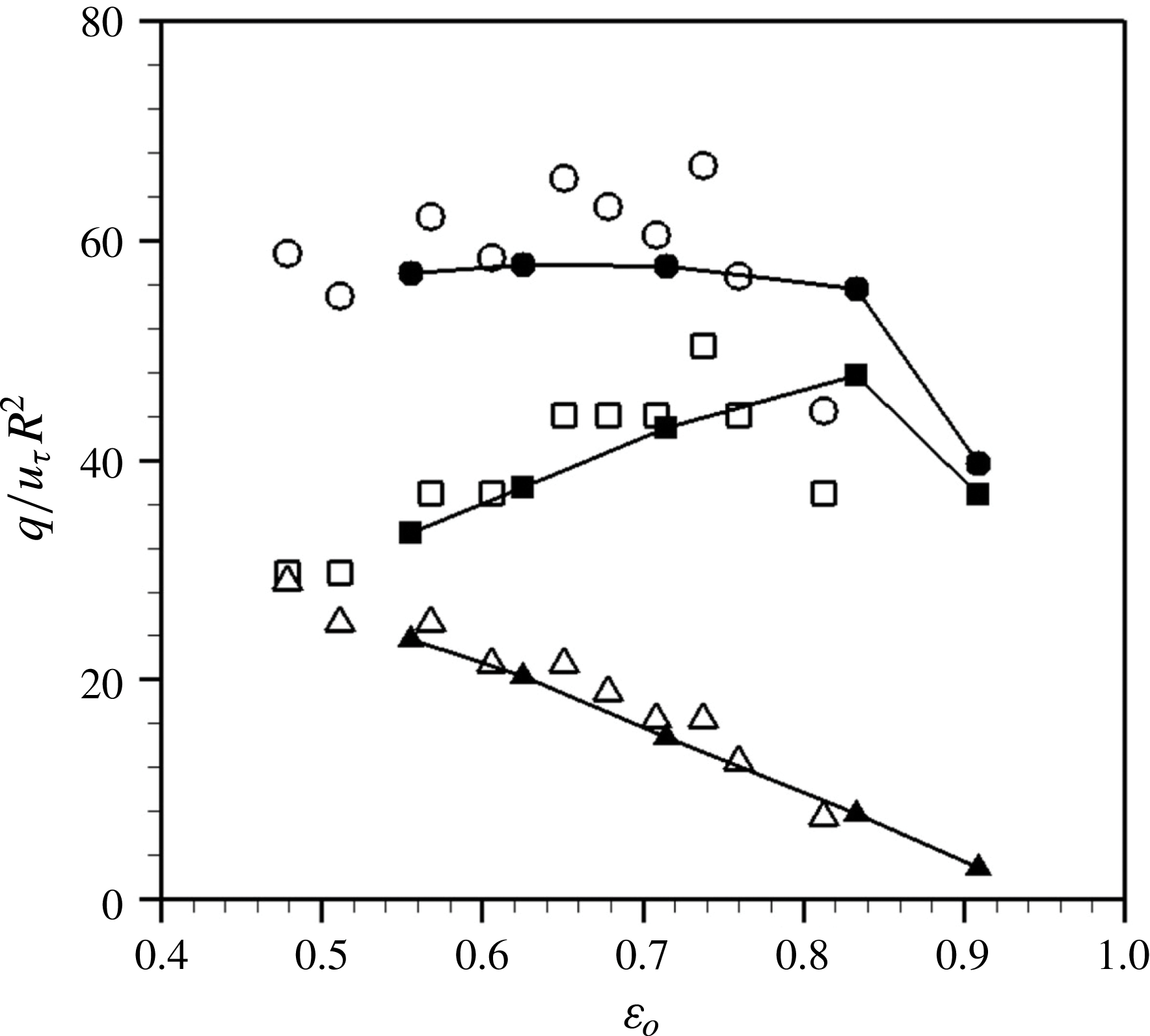
Figure 3 shows the variations of oil, water and total volume flow rates with the oil holdup
 $\unicode[STIX]{x1D700}_{o}(=V_{o}/V)$
, together with the experimental results of Vanegas Prada & Bannwart (Reference Vanegas Prada and Bannwart2001). As the oil holdup increases (or the water holdup decreases), the oil volume flow rate first increases, reaches a maximum and then decreases. A reasonable agreement between the present and experimental data for
 $\unicode[STIX]{x1D700}_{o}\leqslant 0.71$
is observed. Note that the experimental data contain fluctuations of total volume flow rate at low
 $\unicode[STIX]{x1D700}_{o}$
values. Since long wave components of the phase interface appear at low
 $\unicode[STIX]{x1D700}_{o}$
values (see later figures 12 and 13), the flow-developing length should be long enough. The experimental data were measured at approximately 60 to
 $120R$
away from an inlet, which might be not long enough to reach a fully developed region, whereas the present simulation ran over about
 $400R$
at which the flow reached a statistically steady state. However, the agreement becomes poor at high oil holdups such as at
 $\unicode[STIX]{x1D700}_{o}=0.83$
. This disagreement cannot be disregarded, because maximum oil volume flow rate occurs around
 $\unicode[STIX]{x1D700}_{o}=0.83$
in our simulation but at
 $\unicode[STIX]{x1D700}_{o}\approx 0.71$
in the previous experiment. For a high oil holdup, oil frequently sticks to the wall due to narrow water region, which significantly increases the pressure drop (Bai et al.
Reference Bai, Chen and Joseph1992; Arney et al.
Reference Arney, Bai, Guevara, Joseph and Liu1993). This oil sticking is adhesion rather than a hydrodynamic effect (Arney et al.
Reference Arney, Ribeiro, Guevara, Bai and Joseph1996). The present simulation does not consider these chemical procedures, and thus there is a difference in the oil volume flow rate at a very high oil holdup. For this reason, we investigate the flow at
 $\unicode[STIX]{x1D700}_{o}=0.71$
in detail (rather than at
 $\unicode[STIX]{x1D700}_{o}=0.83$
) at which the oil volume flow rate is high in the experiment and is well predicted by the present numerical simulation.
Variations of the volume flow rates with the oil holdup: present simulation (▴, water; ▪, oil; ●, their sum); Vanegas Prada & Bannwart (Reference Vanegas Prada and Bannwart2001, experiment) at
 $Re_{\unicode[STIX]{x1D70F}}\approx 720$
(▵, water; ▫, oil; ○, their sum). The data of Vanegas Prada & Bannwart (Reference Vanegas Prada and Bannwart2001) are taken from the PhD thesis of Vanegas Prada (Reference Vanegas Prada1999).

When high viscosity oil alone flows in a pipe (
 $\unicode[STIX]{x1D700}_{o}=1$
) at the same wall friction (
 $Re_{\unicode[STIX]{x1D70F},o}=\unicode[STIX]{x1D70C}_{o}u_{\unicode[STIX]{x1D70F},o}R/\unicode[STIX]{x1D707}_{o}=Re_{\unicode[STIX]{x1D70F}}(\unicode[STIX]{x1D707}_{w}/\unicode[STIX]{x1D707}_{o})(\unicode[STIX]{x1D70C}_{o}/\unicode[STIX]{x1D70C}_{w})^{0.5}\approx 0.040$
, where
 $Re_{\unicode[STIX]{x1D70F},o}$
and
 $u_{\unicode[STIX]{x1D70F},o}=\sqrt{\overline{\unicode[STIX]{x1D70F}}_{w}/\unicode[STIX]{x1D70C}_{o}}$
are the friction Reynolds number and friction velocity of oil, respectively), the volume flow rate of oil is
 $q_{o}/u_{\unicode[STIX]{x1D70F},o}R^{2}\approx 0.032$
which is orders of magnitude smaller than that of the core-annular flow,
 $q_{o}/u_{\unicode[STIX]{x1D70F}}R^{2}\approx 30{-}50$
(figure 3). Therefore, the core-annular flow is required to transport high viscosity oil. On the other hand, when water flows alone (
 $\unicode[STIX]{x1D700}_{o}=0$
), the volume flow rate is
 $q_{w}/u_{\unicode[STIX]{x1D70F}}R^{2}\approx 56.4$
(
 $Re_{\unicode[STIX]{x1D70F}}=685$
: Wu, Baltzer & Adrian Reference Wu, Baltzer and Adrian2012). This value is comparable to the total volume flow rate of the core-annular flow,
 $(q_{w}+q_{o})/u_{\unicode[STIX]{x1D70F}}R^{2}$
. The total volume flow rate is nearly constant at low to relatively high
 $\unicode[STIX]{x1D700}_{o}$
values but rapidly decreases at high
 $\unicode[STIX]{x1D700}_{o}$
values for
 $\unicode[STIX]{x1D700}_{o}>0.83$
, whereas, with increasing
 $\unicode[STIX]{x1D700}_{o}$
, the volume flow rate of oil increases and then rapidly decreases, but that of water monotonically decreases. Note that the oil volume flow rate at
 $\unicode[STIX]{x1D700}_{o}=0.91$
is much lower than its maximum at
 $\unicode[STIX]{x1D700}_{o}=0.83$
, because the water region is so narrow that the core reaches very close to the pipe wall and suffers from high wall shear stress. Therefore, it is not practical to keep increasing
 $\unicode[STIX]{x1D700}_{o}$
because the amount of oil delivery decreases from its maximum value.
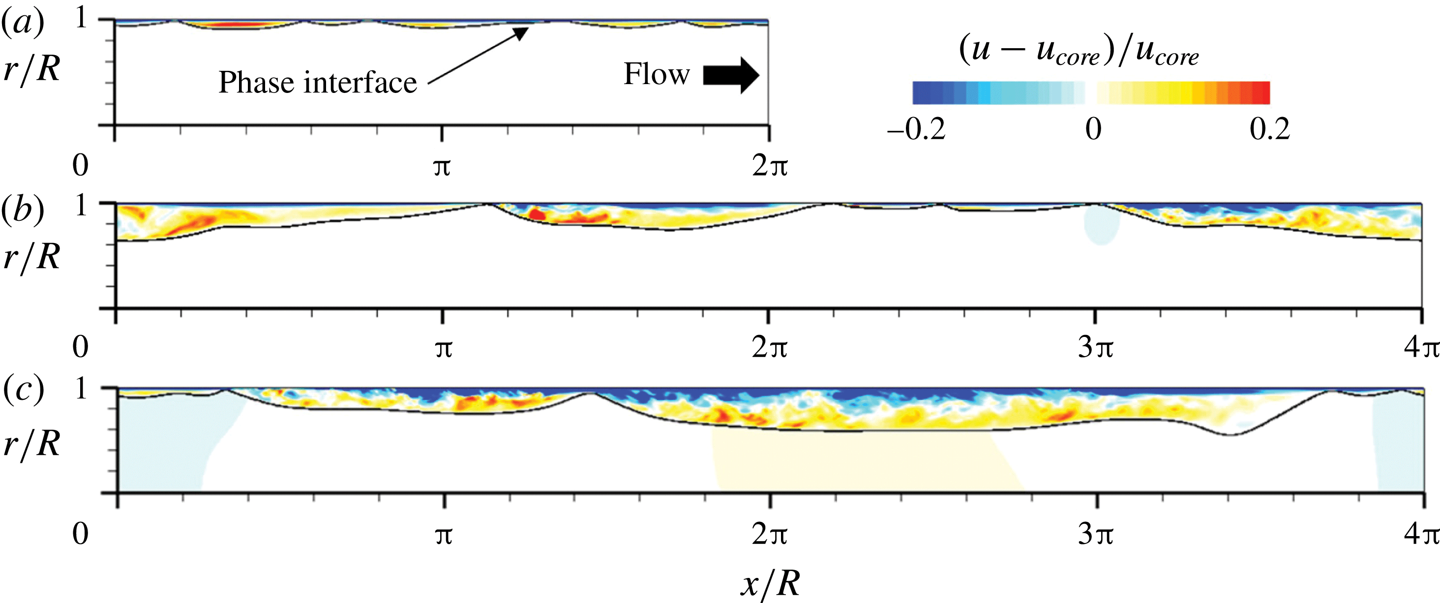
Contours of the instantaneous streamwise velocity relative to the core velocity: (a)
 $\unicode[STIX]{x1D700}_{o}=0.91$
; (b)
 $0.71$
; (c)
 $0.56$
.

Figure 4 shows the contours of the instantaneous streamwise velocity relative to the core velocity for
 $\unicode[STIX]{x1D700}_{o}=0.91,0.71$
and
 $0.56$
, respectively. The core velocity,
 $u_{core}(=\int \!u\,\text{d}V_{o}/V_{o})$
, is the oil velocity averaged over the volume occupied by oil and is related to the superficial velocity of oil as
 $u_{core}=j_{o}/\unicode[STIX]{x1D700}_{o}$
. As shown in this figure, the core region contains nearly zero relative velocity, indicating that the flow in the core region is almost a plug flow moving at the speed of
 $u_{core}$
and has nearly zero velocity fluctuations (e.g. their root-mean-square (r.m.s.) values are less than
 $0.02u_{core}$
for
 $\unicode[STIX]{x1D700}_{o}=0.71$
) due to the high viscosity of oil. As the core region moves at
 $u_{core}$
and deforms very slowly because of its high viscosity (Bai et al.
Reference Bai, Kelkar and Joseph1996), the phase interface behaves like a slowly deforming wavy wall. The water flow in the annulus may be characterized as a Poiseuille–Couette flow such that the top-driven velocity is
 $u_{core}$
and the mean pressure gradient excluding the buoyancy is
 $-\text{d}P/\text{d}x_{annulus}=-\text{d}P/\text{d}x-\unicode[STIX]{x1D70C}_{w}g=2\overline{\unicode[STIX]{x1D70F}}_{w}/R-(\unicode[STIX]{x1D70C}_{w}-\unicode[STIX]{x1D70C}_{o})\unicode[STIX]{x1D700}_{o}g$
. Since the non-dimensional pressure gradient,
 $\unicode[STIX]{x1D6F1}_{c}=(-\text{d}P/\text{d}x_{annulus})(R-h_{avg})/(\unicode[STIX]{x1D70C}_{w}u_{core}^{2})$
, is quite small (
 ${\leqslant}7.2\times 10^{-4}$
), the flow in the annulus is close to Couette flow (Polderman, Velraeds & Knol Reference Polderman, Velraeds and Knol1986). For
 $\unicode[STIX]{x1D700}_{o}=0.91$
, the Reynolds number based on the mean water height is very low, i.e.
 $Re_{c}=u_{core}(R-h_{avg})/\unicode[STIX]{x1D708}_{w}\approx 430$
, and thus near-wall streamwise vortical structures are hardly observable. For lower oil holdups (
 $\unicode[STIX]{x1D700}_{o}\leqslant 0.83$
),
 $Re_{c}\approx 1150{-}3550$
and the flow in the annular region occupied by water becomes turbulent. With decreasing
 $\unicode[STIX]{x1D700}_{o}$
, the dominant wavelength of the phase interface as well as the average gap size
 $h_{avg}$
increase. The relative velocity in the water region in a reference frame moving with
 $u_{core}$
is positive and negative near the phase interface and the wall, respectively, which is also observed in laminar core-annular flows (Bai et al.
Reference Bai, Kelkar and Joseph1996; Li & Renardy Reference Li and Renardy1999). This phenomenon is further discussed later in this paper.
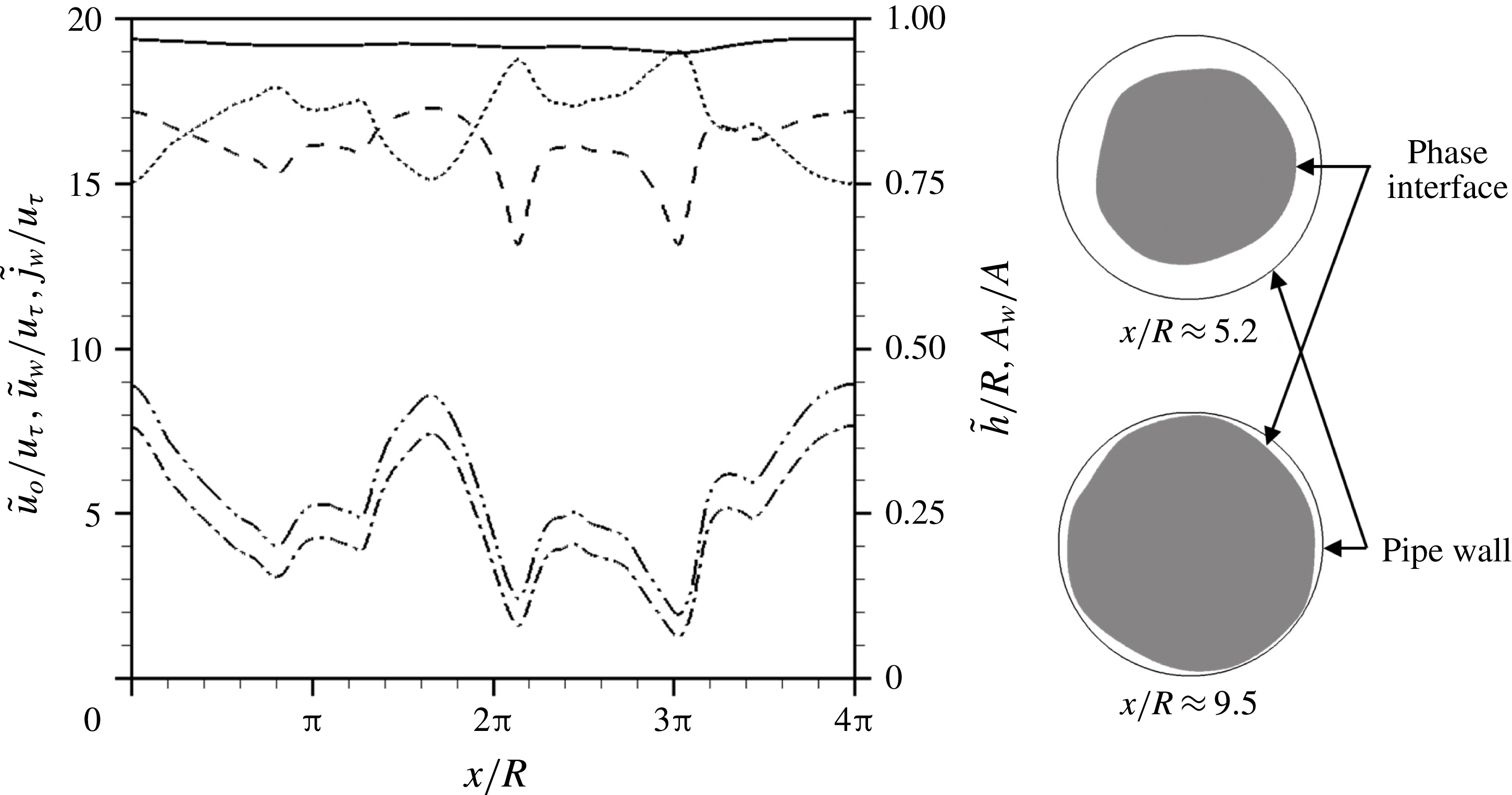
Streamwise distributions of the instantaneous bulk velocities of oil and water (
 $\tilde{u} _{o}(x)$
and
 $\tilde{u} _{w}(x)$
, respectively), superficial velocity of water (
 $\tilde{j}_{w}(x)$
), half of the hydraulic diameter of the phase interface (
 $\tilde{h}$
) and the ratio of instantaneous water area to the pipe cross-sectional area (
 $A_{w}/A$
) for
 $\unicode[STIX]{x1D700}_{o}=0.71$
at the same instant as in figure 4(b), together with the cross-sectional shapes of instantaneous phase interface at two different streamwise locations: ——,
 $\tilde{u} _{o}/u_{\unicode[STIX]{x1D70F}}$
; - - - -,
 $\tilde{u} _{w}/u_{\unicode[STIX]{x1D70F}}$
; – - – - –,
 $\tilde{j}_{w}/u_{\unicode[STIX]{x1D70F}}$
; – -- – -- –,
 $A_{w}/A$
;
 $\cdots \cdots$
,
 $\tilde{h}$
.

Figure 5 shows the streamwise distributions of the instantaneous bulk velocities of oil and water (
 $\tilde{u} _{o}$
and
 $\tilde{u} _{w}$
), superficial velocity of water (
 $\tilde{j}_{w}$
), half of the hydraulic diameter of the core (
 $\tilde{h}=2A_{o}/{\mathcal{P}}$
;
 $A_{o}$
and
 ${\mathcal{P}}$
are the instantaneous area and perimeter of the core, respectively) and the ratio of instantaneous water area to the pipe cross-sectional area (
 $A_{w}/A$
) for
 $\unicode[STIX]{x1D700}_{o}=0.71$
, together with the cross-sectional shapes of instantaneous phase interface at two different streamwise locations, where
 $\tilde{u} _{o}=\int \!u(1-\unicode[STIX]{x1D713})\,\text{d}A/\!\int (1-\unicode[STIX]{x1D713})\,\text{d}A$
,
 $\tilde{u} _{w}=\int \!u\unicode[STIX]{x1D713}\,\text{d}A/\!\int \!\unicode[STIX]{x1D713}\,\text{d}A$
,
 $\tilde{j}_{w}=\int \!u\unicode[STIX]{x1D713}\,\text{d}A/\!\int \!\text{d}A$
and
 $\tilde{h}=\int _{0}^{2\unicode[STIX]{x03C0}}\!h^{2}\,\text{d}\unicode[STIX]{x1D703}/\!\int _{0}^{2\unicode[STIX]{x03C0}}\!h\,\text{d}\unicode[STIX]{x1D703}$
. As shown in this figure,
 $\tilde{u} _{w}$
is smaller than
 $\tilde{u} _{o}$
at all the streamwise locations, indicating that the oil overall drags the water. However, ahead of a crest (local maximum
 $h$
), water locally drives oil near the phase interface (see the red contours in figure 4). The instantaneous superficial velocity of water
 $\tilde{j}_{w}$
varies in the streamwise direction because of non-zero radial velocity fluctuations of the phase interface. With decreasing
 $A_{w}/A$
,
 $\tilde{u} _{w}$
and
 $\tilde{j}_{w}(=\tilde{u} _{w}(A_{w}/A))$
decrease. When the crests of the phase interface are located very near the wall, water is almost trapped between the crests and
 $\tilde{j}_{w}$
rapidly decreases. This water trapping inside the wave valley between the crests was also noticed in laminar core-annular flows (Bai et al.
Reference Bai, Kelkar and Joseph1996; Li & Renardy Reference Li and Renardy1999; Kouris & Tsamopoulos Reference Kouris and Tsamopoulos2002).
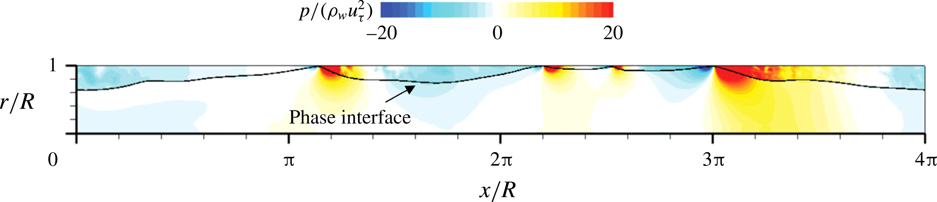
Contours of the instantaneous pressure fluctuations (
 $\unicode[STIX]{x1D700}_{o}=0.71$
) at the same instant as in figure 4(b).

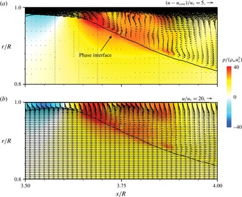
Instantaneous velocity vectors and contours of the instantaneous pressure fluctuations near the crest of the interface (
 $\unicode[STIX]{x1D700}_{o}=0.71$
): (a) in a reference frame moving with the core velocity; (b) in a stationary reference frame. Here, the time is same as that in figure 4(b).

Figure 6 shows the contours of the instantaneous pressure fluctuations for
 $\unicode[STIX]{x1D700}_{o}=0.71$
. Since oil moves like a solid body at the speed of
 $u_{core}$
and drives the water, the pressures ahead of and behind the crests are high and low, respectively. The pressure in the valley region is negative and is more or less uniform. Figures 7(a) and (b) show the instantaneous velocity vectors near the crest of the phase interface in a reference frame moving with the core velocity and in a stationary reference frame, respectively, together with the contours of the instantaneous pressure fluctuations for
 $\unicode[STIX]{x1D700}_{o}=0.71$
. The discontinuity in the pressure fluctuations across the phase interface is due to the surface tension. In a reference frame moving with
 $u_{core}$
(figure 7
a), the wall moves upstream, and flow impinges on the front part of the crest, creating high pressure and forming a recirculation bubble there. Also, a positive relative velocity exists above the phase interface in the valley region. In a stationary reference frame (figure 7
b), the velocity field of water is more or less uniform except near the wall and the crest. Near the wall, the boundary layer grows in the streamwise direction, whereas the velocity near the crest rapidly changes in the radial and streamwise directions. The velocity gradient at the phase interface is very small except on the crest. Figure 8 shows the instantaneous phase interface and vortical structures in the annulus for
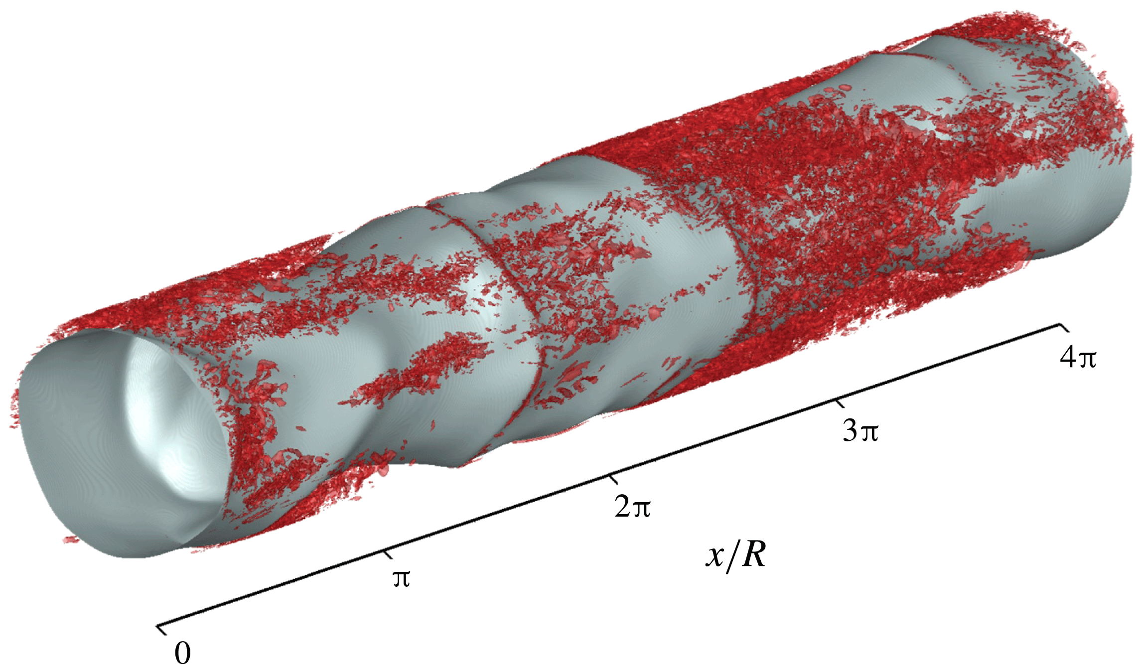
 $\unicode[STIX]{x1D700}_{o}=0.71$
. Vortical structures evolve near the wall, but differ from those of a fully developed pipe flow. They exist at the locations ahead of the crests and in the valley regions, but few appear right behind the crests. This is quite interesting because one may expect more vortices behind a crest in the form of wake. However, the gap between the crest and wall is so narrow that the vortices are weaken and flow does not evolve into turbulent shear layer behind the crest.
Instantaneous phase interface and vortical structures (
 $\unicode[STIX]{x1D706}_{2}=-200\,000$
(Jeong & Hussain Reference Jeong and Hussain1995)) in the annulus (
 $\unicode[STIX]{x1D700}_{o}=0.71$
).

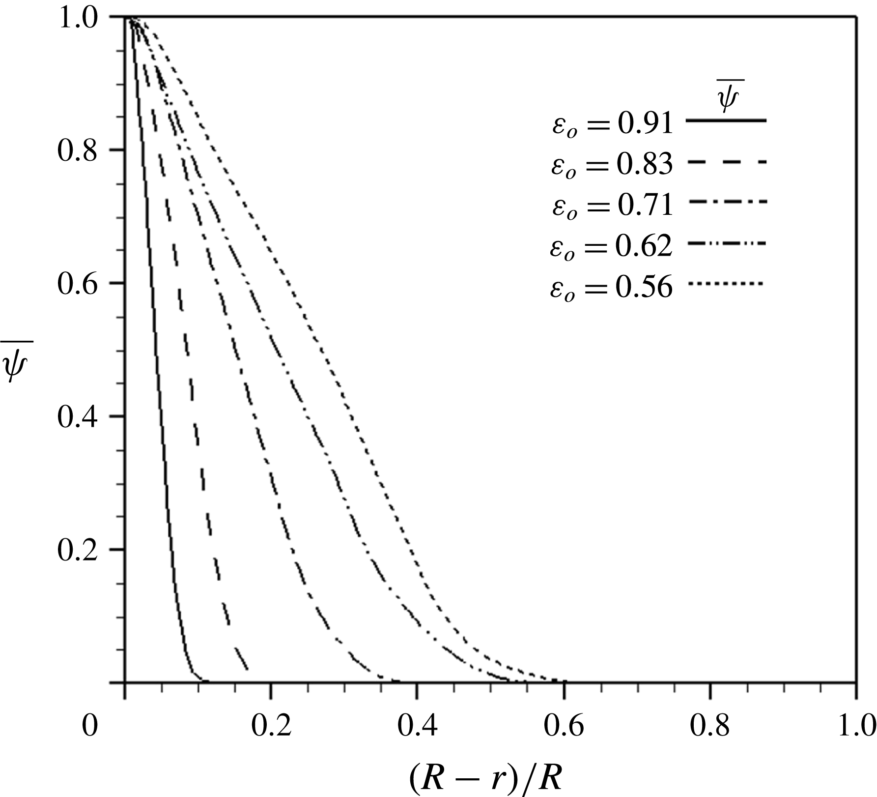
Distributions of the mean water volume fraction in the radial direction.

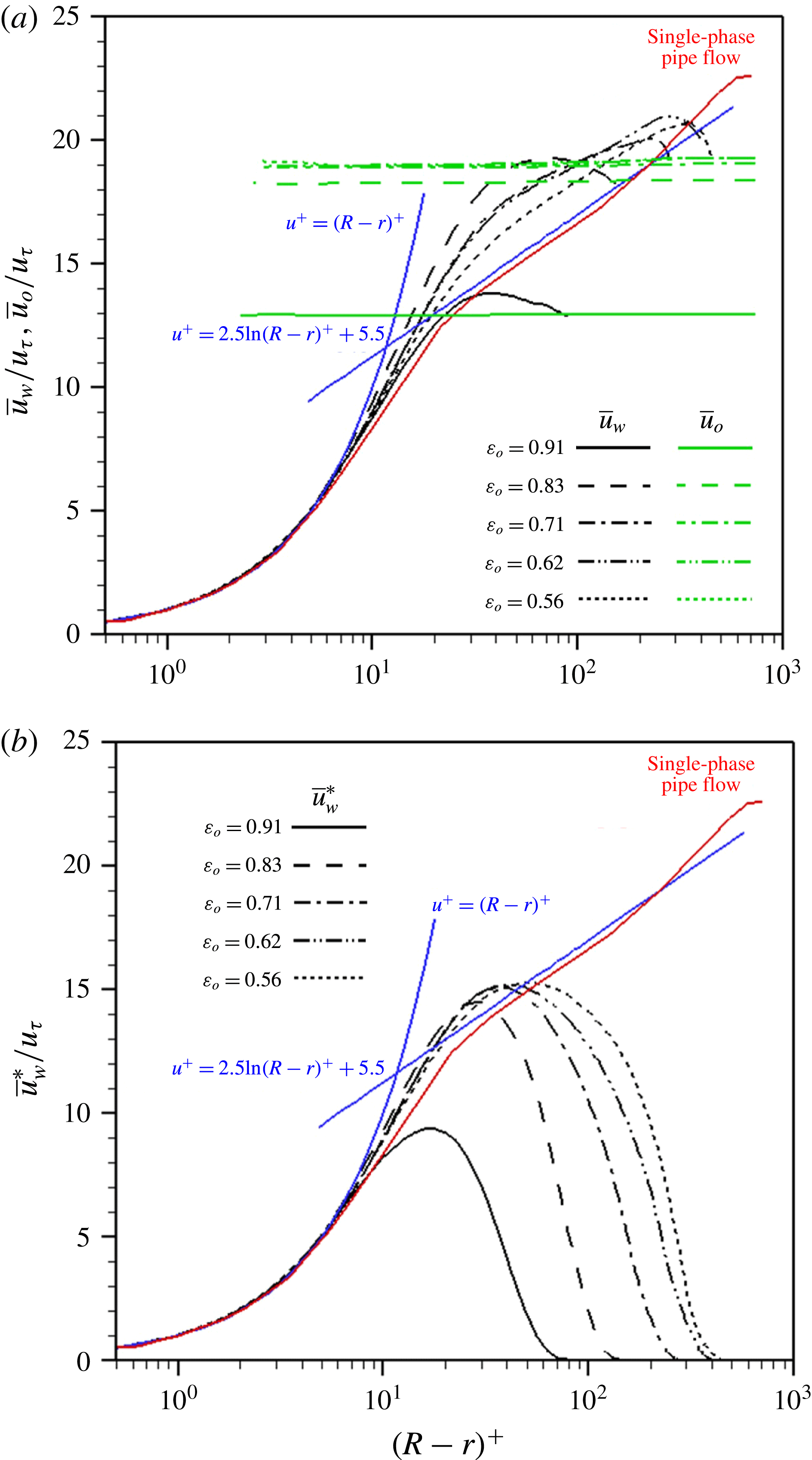
Profiles of the mean streamwise velocities of water and oil for different oil holdups: (a)
 $\overline{u}_{w}$
and
 $\overline{u}_{o}$
; (b)
 $\overline{u}_{w}^{\ast }(=\overline{u}_{w}\overline{\unicode[STIX]{x1D713}})$
. The red line denotes the mean velocity profile of a single-phase pipe flow at
 $Re_{\unicode[STIX]{x1D70F}}=685$
(Wu et al.
Reference Wu, Baltzer and Adrian2012) and the log law of
 $u^{+}=2.5\ln (R-r)^{+}+5.5$
is from Eggels et al. (Reference Eggels, Unger, Weiss, Westerweel, Adrian, Friedrich and Nieuwstadt1994).

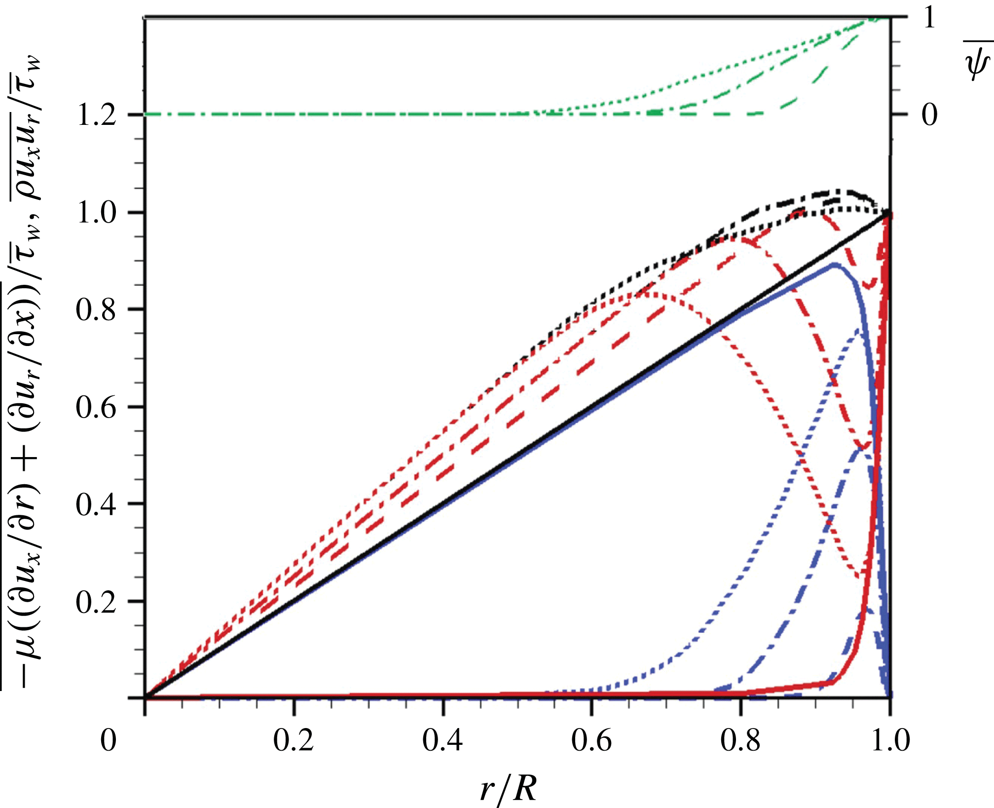
Radial distributions of shear stresses in the mean streamwise momentum equation (blue lines, Reynolds shear stress; red lines, viscous shear stress; black lines, total shear stress) and the mean water volume fraction (green lines). - - - -,
 $\unicode[STIX]{x1D700}_{o}=0.83$
; – - – - –,
 $0.71$
;
 $\cdots \cdots$
,
 $0.56$
; ——, single-phase pipe flow at
 $Re_{\unicode[STIX]{x1D70F}}=685$
(Wu et al.
Reference Wu, Baltzer and Adrian2012).

Due to the wavy phase interface, there is an intermittent region near the phase interface where the fluid changes from water to oil in time or vice versa. In this region, the interaction between the water flow and phase interface is quite active, and heavily influences the flow statistics (see figures 10 and 11). Figure 9 shows the mean water volume fraction
 $$\begin{eqnarray}\displaystyle & \displaystyle \overline{\unicode[STIX]{x1D713}}(r)={\displaystyle \frac{\displaystyle \iiint \unicode[STIX]{x1D713}(x,r,\unicode[STIX]{x1D703},t)\,\text{d}\unicode[STIX]{x1D703}\,\text{d}x\,\text{d}t}{\displaystyle \iiint \text{d}\unicode[STIX]{x1D703}\,\text{d}x\,\text{d}t}}. & \displaystyle\end{eqnarray}$$
Here,
 $\overline{\unicode[STIX]{x1D713}}=1$
and 0 for water and oil only regions, respectively, and
 $0<\overline{\unicode[STIX]{x1D713}}<1$
for the intermittent region. Note that
 $\overline{\unicode[STIX]{x1D713}}$
does not provide a precise position of the phase interface, but indicates the amount of water in volume fraction. As shown, the region with
 $\overline{\unicode[STIX]{x1D713}}=1$
is located very near the wall, and
 $\overline{\unicode[STIX]{x1D713}}$
decreases linearly with the distance from the wall except for the region with very low
 $\overline{\unicode[STIX]{x1D713}}$
values. Note that, with decreasing
 $\unicode[STIX]{x1D700}_{o}$
, the slope becomes slow and the region of
 $0<\overline{\unicode[STIX]{x1D713}}<1$
becomes wider.
Figure 10(a) shows the profiles of the mean streamwise velocity of water (
 $\overline{u}_{w}$
) and oil (
 $\overline{u}_{o}$
), respectively, for different oil holdups, together with that of a single-phase pipe flow at
 $Re_{\unicode[STIX]{x1D70F}}=685$
(Wu et al.
Reference Wu, Baltzer and Adrian2012):
 $$\begin{eqnarray}\displaystyle & \displaystyle \overline{u}_{w}(r)={\displaystyle \frac{\displaystyle \iiint u(x,r,\unicode[STIX]{x1D703},t)\unicode[STIX]{x1D713}(x,r,\unicode[STIX]{x1D703},t)\,\text{d}\unicode[STIX]{x1D703}\,\text{d}x\,\text{d}t}{\displaystyle \iiint \unicode[STIX]{x1D713}(x,r,\unicode[STIX]{x1D703},t)\,\text{d}\unicode[STIX]{x1D703}\,\text{d}x\,\text{d}t}}, & \displaystyle\end{eqnarray}$$
 $$\begin{eqnarray}\displaystyle & \displaystyle \overline{u}_{o}(r)={\displaystyle \frac{\displaystyle \iiint u(x,r,\unicode[STIX]{x1D703},t)(1-\unicode[STIX]{x1D713}(x,r,\unicode[STIX]{x1D703},t))\,\text{d}\unicode[STIX]{x1D703}\,\text{d}x\,\text{d}t}{\displaystyle \iiint (1-\unicode[STIX]{x1D713}(x,r,\unicode[STIX]{x1D703},t))\,\text{d}\unicode[STIX]{x1D703}\,\text{d}x\,\text{d}t}}. & \displaystyle\end{eqnarray}$$
Since
 $\overline{u}_{w}$
and
 $\overline{u}_{o}$
are the mean velocities obtained with a weight of
 $\unicode[STIX]{x1D713}$
, both velocity profiles co-exist in the intermittent region (
 $0<\overline{\unicode[STIX]{x1D713}}<1$
). For each
 $\unicode[STIX]{x1D700}_{o}$
,
 $\overline{u}_{o}$
is nearly constant (
 ${\approx}u_{core}$
) even very near the wall, but is maximum at the centre and slowly decreases with increasing
 $r$
(it increases again near
 $\overline{\unicode[STIX]{x1D713}}=1$
). The effect of this velocity gradient becomes manifest when it is multiplied by the oil viscosity (see figure 11). With decreasing
 $\unicode[STIX]{x1D700}_{o}$
(under the condition of constant mean pressure gradient),
 $\overline{u}_{o}$
increases but converges a nearly constant value,
 $\overline{u}_{o}/u_{\unicode[STIX]{x1D70F}}\approx 19$
, for
 $\unicode[STIX]{x1D700}_{o}\leqslant 0.71$
. A similar observation of constant
 $\overline{u}_{o}$
was made in the experimental study of Tripathi et al. (Reference Tripathi, Tabor, Singh and Bhattacharya2017) for a horizontal core-annular flow. On the other hand, with increasing wall distance,
 $\overline{u}_{w}$
increases, reaches maximum, and then decreases to
 $\overline{u}_{o}$
. Thus, the peak velocity of water is faster than the oil core velocity, which results from the positive relative velocity ahead of the crest (see figure 6
a). Also,
 $\overline{u}_{w}$
values are very different from that of a single-phase pipe flow. Except for
 $\unicode[STIX]{x1D700}_{o}=0.91$
, the velocity profile shows more upward shift of the log law for higher
 $\unicode[STIX]{x1D700}_{o}$
. With decreasing
 $\unicode[STIX]{x1D700}_{o}$
, the upward shift decreases and the velocity profile approaches that of single-phase pipe flow in the log region. This behaviour is natural because the water region increases with decreasing
 $\unicode[STIX]{x1D700}_{o}$
and thus the water flow becomes more like single-phase pipe flow. The different behaviour for
 $\unicode[STIX]{x1D700}_{o}=0.91$
is owing to the very thin water region. Figure 10(b) shows the mean streamwise velocity of water weighted by the mean water volume fraction,
 $\overline{u}_{w}^{\ast }$
:
 $$\begin{eqnarray}\displaystyle \displaystyle \overline{u}_{w}^{\ast }(r) & = & \displaystyle {\displaystyle \frac{\displaystyle \iiint u(x,r,\unicode[STIX]{x1D703},t)\unicode[STIX]{x1D713}(x,r,\unicode[STIX]{x1D703},t)\,\text{d}\unicode[STIX]{x1D703}\,\text{d}x\,\text{d}t}{\displaystyle \iiint \text{d}\unicode[STIX]{x1D703}\,\text{d}x\,\text{d}t}}\nonumber\\ \displaystyle & = & \displaystyle {\displaystyle \frac{\displaystyle \iiint u(x,r,\unicode[STIX]{x1D703},t)\unicode[STIX]{x1D713}(x,r,\unicode[STIX]{x1D703},t)\,\text{d}\unicode[STIX]{x1D703}\,\text{d}x\,\text{d}t}{\displaystyle \iiint \unicode[STIX]{x1D713}(x,r,\unicode[STIX]{x1D703},t)\,\text{d}\unicode[STIX]{x1D703}\,\text{d}x\,\text{d}t}}{\displaystyle \frac{\displaystyle \iiint \unicode[STIX]{x1D713}(x,r,\unicode[STIX]{x1D703},t)\,\text{d}\unicode[STIX]{x1D703}\,\text{d}x\,\text{d}t}{\displaystyle \iiint \text{d}\unicode[STIX]{x1D703}\,\text{d}x\,\text{d}t}}\nonumber\\ \displaystyle \displaystyle & = & \displaystyle \overline{u}_{w}(r)\overline{\unicode[STIX]{x1D713}}(r).\end{eqnarray}$$
As the distance from the wall increases,
 $\overline{u}_{w}^{\ast }$
increases and then decreases. The reason for the decrease in
 $\overline{u}_{w}^{\ast }$
is that in this region
 $0<\overline{\unicode[STIX]{x1D713}}<1$
and
 $\overline{u}_{w}^{\ast }=\overline{u}_{w}\overline{\unicode[STIX]{x1D713}}$
. This
 $\overline{u}_{w}^{\ast }$
will be used in developing an oil holdup model (see § 3.3).
Figure 11 shows the radial distributions of the Reynolds and viscous shear stresses and their sum of the core-annular and single-phase pipe flows, respectively, together with the mean water volume fraction. The total shear stress of core-annular flow is larger at all radial locations than that of a single-phase pipe flow. Unlike the single-phase pipe flow, the total shear stress profile is not linear due to the body force term:
 $$\begin{eqnarray}\displaystyle & \displaystyle \overline{\unicode[STIX]{x1D70F}}(r)=\overline{\unicode[STIX]{x1D70C}u_{x}u_{r}}-\overline{\unicode[STIX]{x1D707}\left({\displaystyle \frac{\unicode[STIX]{x2202}u_{x}}{\unicode[STIX]{x2202}r}}+{\displaystyle \frac{\unicode[STIX]{x2202}u_{r}}{\unicode[STIX]{x2202}x}}\right)}={\displaystyle \frac{r}{2}}\left(-{\displaystyle \frac{\text{d}P}{\text{d}x}}\right)+{\displaystyle \frac{1}{r}}\int _{0}^{r}(\overline{\unicode[STIX]{x1D70E}\unicode[STIX]{x1D705}\unicode[STIX]{x1D6FF}n_{x}}-\overline{\unicode[STIX]{x1D70C}}g)\,r\,\text{d}r, & \displaystyle\end{eqnarray}$$
where the overbar denotes averaging over the streamwise and azimuthal directions and time. Note that
 $\overline{\unicode[STIX]{x1D70C}u_{x}u_{r}}=\overline{u}_{x}\overline{\unicode[STIX]{x1D70C}u_{r}^{\prime }}+\overline{\unicode[STIX]{x1D70C}u_{x}^{\prime }u_{r}^{\prime }}\approx \overline{\unicode[STIX]{x1D70C}u_{x}^{\prime }u_{r}^{\prime }}$
because
 $\unicode[STIX]{x1D70C}_{w}/\unicode[STIX]{x1D70C}_{o}=1.036$
, and the surface tension term is negligibly small (e.g.
 $|1/r\int _{0}^{r}\overline{\unicode[STIX]{x1D70E}\unicode[STIX]{x1D705}\unicode[STIX]{x1D6FF}n_{x}}\,r\,\text{d}r|_{max}<0.012\overline{\unicode[STIX]{x1D70F}}_{w}$
for
 $\unicode[STIX]{x1D700}_{o}=0.71$
) as compared to other terms. In a single-phase pipe flow, the Reynolds shear stress is much larger than the viscous shear stress except very near the wall. However, in the core-annular flow, the viscous shear stress is dominant in the water-free region (
 $\overline{\unicode[STIX]{x1D713}}=0$
) and increases in the radial direction, whereas, in the region of
 $\overline{\unicode[STIX]{x1D713}}\neq 0$
, the viscous shear stress rapidly decreases, reaches local minimum, and increases again in the radial direction. The Reynolds shear stress is nearly zero in the water-free region due to the core flow characteristics, but rapidly increases in the region of
 $\overline{\unicode[STIX]{x1D713}}\neq 0$
and decreases to zero at the wall. The large magnitudes of the viscous shear stress in the water-free region are due to the high oil viscosity (17600 times that of water), although the velocity gradient in the core region is very small. The viscous (or total) shear stress in this region (
 $\overline{\unicode[STIX]{x1D713}}=0$
) is balanced by the mean pressure gradient and buoyancy force (nearly zero Reynolds shear stress in this region): using (2.16),
 $$\begin{eqnarray}\displaystyle \displaystyle \overline{\unicode[STIX]{x1D70F}}_{oil}(r)={\displaystyle \frac{r}{2}}\left(-{\displaystyle \frac{\text{d}P}{\text{d}x}}-\unicode[STIX]{x1D70C}_{o}g\right) & = & \displaystyle {\displaystyle \frac{r}{2}}\left[\left({\displaystyle \frac{2\overline{\unicode[STIX]{x1D70F}}_{w}}{R}}+{\displaystyle \frac{1}{V}}\int \unicode[STIX]{x1D70C}g\,\text{d}V\right)-\unicode[STIX]{x1D70C}_{o}g\right]\nonumber\\ \displaystyle & = & \displaystyle {\displaystyle \frac{r}{2}}\left[{\displaystyle \frac{2\overline{\unicode[STIX]{x1D70F}}_{w}}{R}}+(\unicode[STIX]{x1D70C}_{w}-\unicode[STIX]{x1D70C}_{o})g(1-\unicode[STIX]{x1D700}_{o})\right].\end{eqnarray}$$
The slopes of the viscous (or total) shear stress in the water-free region predicted by (3.6) for
 $\unicode[STIX]{x1D700}_{o}=0.83,0.71$
and
 $0.56$
are
 $1.15,1.25$
and
 $1.38\overline{\unicode[STIX]{x1D70F}}_{w}/R$
, respectively, which are accurately predicted by the present simulations (figure 11). With decreasing
 $\unicode[STIX]{x1D700}_{o}$
, local minimum viscous shear and maximum Reynolds shear stresses in the region of
 $\overline{\unicode[STIX]{x1D713}}\neq 0$
become smaller and bigger, respectively, and their behaviours very near the wall are similar to those of the single-phase pipe flow. For
 $\unicode[STIX]{x1D700}_{o}=0.91$
, the Reynolds shear stress is almost zero (non-turbulent annulus) and the viscous shear stress is dominant for both core and annular regions (not shown in the figure).
3.2 Phase interface wave
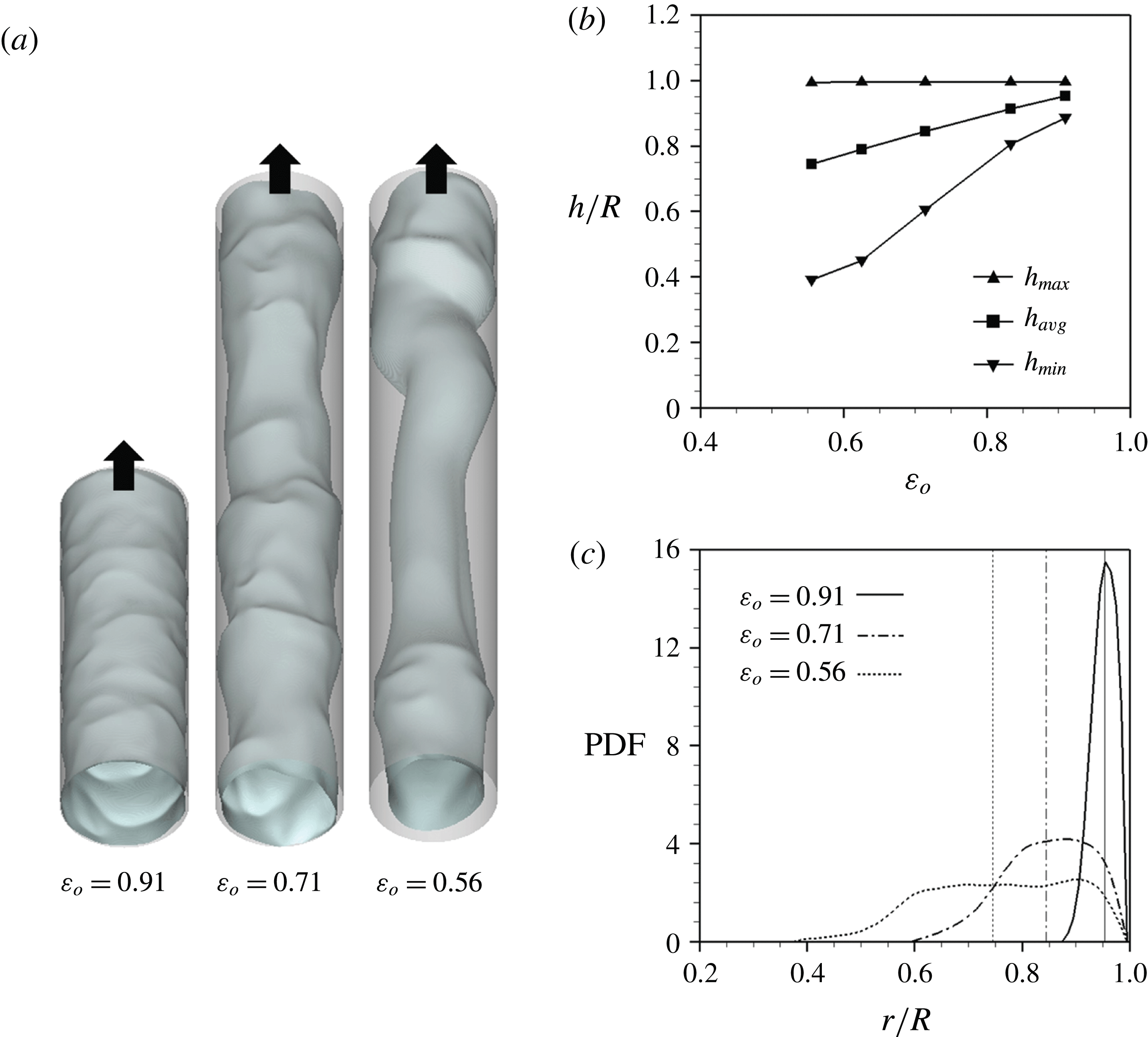
Figure 12 shows the characteristics of the phase interface. The phase interfaces consist of different streamwise and azimuthal wavenumber components for different oil holdups. For example, the streamwise wavelength of the phase interface increases with decreasing
 $\unicode[STIX]{x1D700}_{o}$
. Also, the instantaneous phase interface located near the wall has a small wavelength and amplitude, but the one away from the wall has a large wavelength and amplitude, as seen for
 $\unicode[STIX]{x1D700}_{o}=0.56$
in figure 12(a) (see also Tripathi et al. (Reference Tripathi, Tabor, Singh and Bhattacharya2017) for a horizontal core-annular flow). More detailed analysis of its wave characteristics is given below. As the volume of each fluid is prescribed with given oil holdup, the average location of the phase interface is predetermined as listed in table 1. The maximum radial location of the phase interface (
 $h_{max}$
) is near the wall, but the minimum location (
 $h_{min}$
) decreases with decreasing
 $\unicode[STIX]{x1D700}_{o}$
(figure 12
b), indicating that the wave amplitude of the phase interface is larger at lower
 $\unicode[STIX]{x1D700}_{o}$
. This was also observed in the previous experiment by Rodriguez & Bannwart (Reference Rodriguez and Bannwart2006). The probability density function (PDF) of the phase interface location becomes broader and moves towards the pipe centre with decreasing
 $\unicode[STIX]{x1D700}_{o}$
(figure 12
c), which confirms the behaviours discussed from the instantaneous phase interface and table 1 (i.e. with decreasing
 $\unicode[STIX]{x1D700}_{o}$
, its mean location moves away for the wall and its fluctuation amplitude becomes larger). Except for
 $\unicode[STIX]{x1D700}_{o}=0.91$
, the PDFs have flat profiles near the mean locations.
Characteristics of the phase interfaces: (a) instantaneous shapes; (b) their maximum, average and minimum radii; (c) PDFs of the radial location of the phase interfaces. In (c), thin vertical lines indicate the mean locations of the phase interface for given oil holdups.

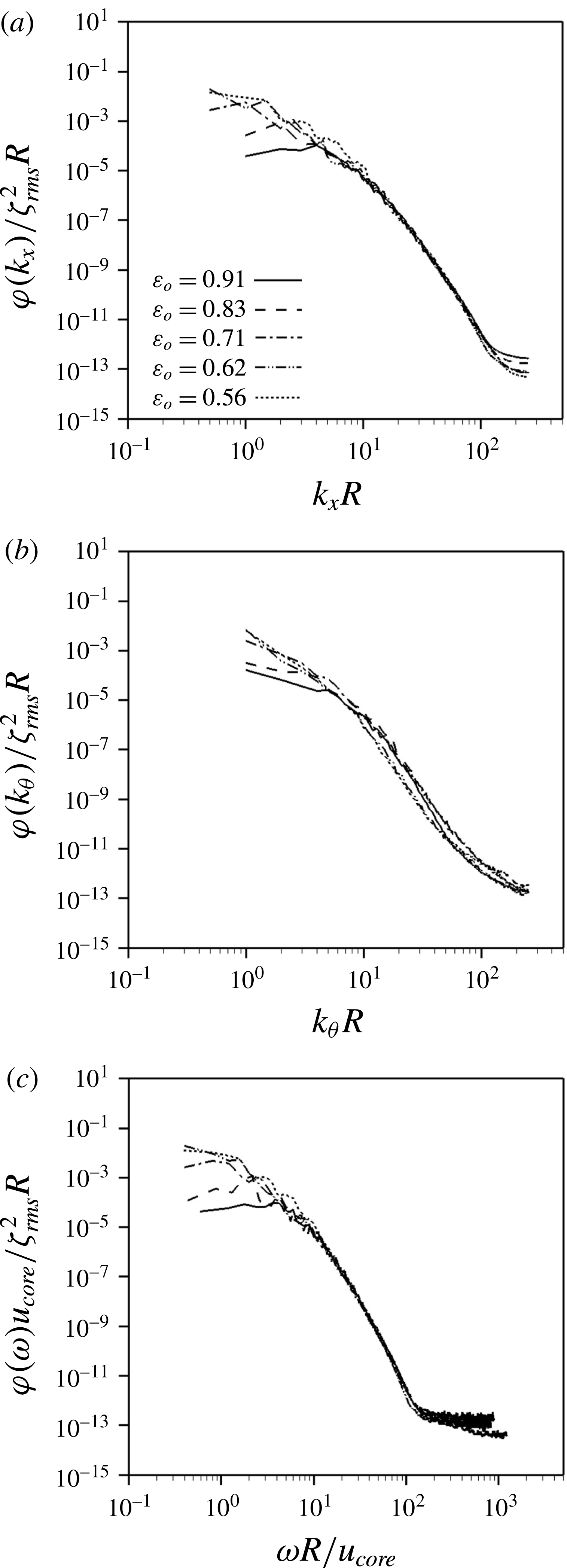
One-dimensional spectra of the phase interface amplitude: (a) streamwise wavenumber; (b) azimuthal wavenumber; (c) frequency.

The wave characteristics of the phase interfaces are investigated from their power spectra. For this purpose, we perform additional computations with the sampling resolution of
 $\unicode[STIX]{x0394}t=0.0002R/u_{\unicode[STIX]{x1D70F}}$
(
 $\unicode[STIX]{x0394}t\approx 0.0026R/u_{core}$
) during the period of
 $T=1.6384R/u_{\unicode[STIX]{x1D70F}}\approx 20.12R/u_{core}$
for
 $\unicode[STIX]{x1D700}_{o}=0.91$
, and with
 $\unicode[STIX]{x0394}t\approx 0.0038R/u_{core}$
during
 $T=31.4R/u_{core}$
for
 $\unicode[STIX]{x1D700}_{o}\leqslant 0.83$
, respectively. Each of these periods is divided into three overlapping segments with 50 % overlap (for more details, see Choi & Moin Reference Choi and Moin1990). The ranges of the streamwise and azimuthal wavenumbers are
 $0\leqslant k_{x}\leqslant 255/R~(\unicode[STIX]{x0394}k_{x}=1/R)$
for
 $\unicode[STIX]{x1D700}_{o}=0.91$
and 0.83 and
 $0\leqslant k_{x}\leqslant 255.5/R~(\unicode[STIX]{x0394}k_{x}=0.5/R)$
for
 $\unicode[STIX]{x1D700}_{o}\leqslant 0.71$
, and
 $0\leqslant k_{\unicode[STIX]{x1D703}}\leqslant 255/R$
 $(\unicode[STIX]{x0394}k_{\unicode[STIX]{x1D703}}=1/R)$
, respectively, where
 $k_{x}$
and
 $k_{\unicode[STIX]{x1D703}}$
are the streamwise and azimuthal wavenumbers. Figure 13 shows one-dimensional wavenumber spectra,
 $\unicode[STIX]{x1D711}(k_{x})$
and
 $\unicode[STIX]{x1D711}(k_{\unicode[STIX]{x1D703}})$
, and frequency spectrum,
 $\unicode[STIX]{x1D711}(\unicode[STIX]{x1D714})$
, of the phase interface amplitude which satisfy the following condition:
 $$\begin{eqnarray}\displaystyle & \displaystyle \int _{0}^{\infty }\unicode[STIX]{x1D711}(k_{x})\,\text{d}k_{x}=\int _{0}^{\infty }\unicode[STIX]{x1D711}(k_{\unicode[STIX]{x1D703}})\,\text{d}k_{\unicode[STIX]{x1D703}}=\int _{0}^{\infty }\unicode[STIX]{x1D711}(\unicode[STIX]{x1D714})\,\text{d}\unicode[STIX]{x1D714}=\unicode[STIX]{x1D701}_{rms}^{2}, & \displaystyle\end{eqnarray}$$
where
 $\unicode[STIX]{x1D714}$
is the frequency, and
 $\unicode[STIX]{x1D701}_{rms}$
is the root-mean-square (r.m.s.) fluctuation of the phase interface amplitude
 $\unicode[STIX]{x1D701}~(=h{-}h_{avg})$
. The phase interface amplitude has broadband spectra, which is very different from the observations of one-wavenumber peak in laminar core-annular flows (Bai et al.
Reference Bai, Kelkar and Joseph1996; Li & Renardy Reference Li and Renardy1999), and of smooth waves from RANS simulations of turbulent core-annular flows (Ghosh et al.
Reference Ghosh, Das and Das2010; Ingen Housz et al.
Reference Ingen Housz, Ooms, Henkes, Pourquie, Kidess and Radhakrishnan2017; Shi et al.
Reference Shi, Gourma and Yeung2017). With decreasing
 $\unicode[STIX]{x1D700}_{o}$
, low wavenumbers contain more power, as observed by previous experiments (Bai Reference Bai1995; Rodriguez & Bannwart Reference Rodriguez and Bannwart2006), but the powers at intermediate and high wavenumbers are similar. In the case of the azimuthal wavenumber spectra (figure 13
b), the largest power occurs at the smallest wavenumber,
 $k_{\unicode[STIX]{x1D703}}=1/R$
, whose corresponding wavelength is the pipe circumference. The frequency spectra show a behaviour similar to the streamwise wavenumber spectra, indicating the convective nature of the phase interface.
The convection velocity can be obtained from the power spectrum (Wills Reference Wills1970; Choi & Moin Reference Choi and Moin1990):
 $$\begin{eqnarray}\displaystyle & \displaystyle U_{conv}(k_{x})=-{\displaystyle \frac{\unicode[STIX]{x1D714}(k_{x})}{k_{x}}}, & \displaystyle\end{eqnarray}$$
where
 $\unicode[STIX]{x1D714}(k_{x})$
is obtained from
 $$\begin{eqnarray}\displaystyle & \displaystyle \left.{\displaystyle \frac{\unicode[STIX]{x2202}\unicode[STIX]{x1D6F7}(k_{x},\unicode[STIX]{x1D714})}{\unicode[STIX]{x2202}\unicode[STIX]{x1D714}}}\right|_{\unicode[STIX]{x1D714}=\unicode[STIX]{x1D714}(k_{x})}=0, & \displaystyle\end{eqnarray}$$
and
 $\unicode[STIX]{x1D6F7}(k_{x},\unicode[STIX]{x1D714})$
is the two-dimensional power spectrum. A quadratic polynomial is used to find
 $\unicode[STIX]{x1D714}(k_{x})$
in (3.9) (Kang, Moin & Iaccarino Reference Kang, Moin and Iaccarino2008). Figure 14 shows the variation of the convection velocity normalized by
 $u_{core}$
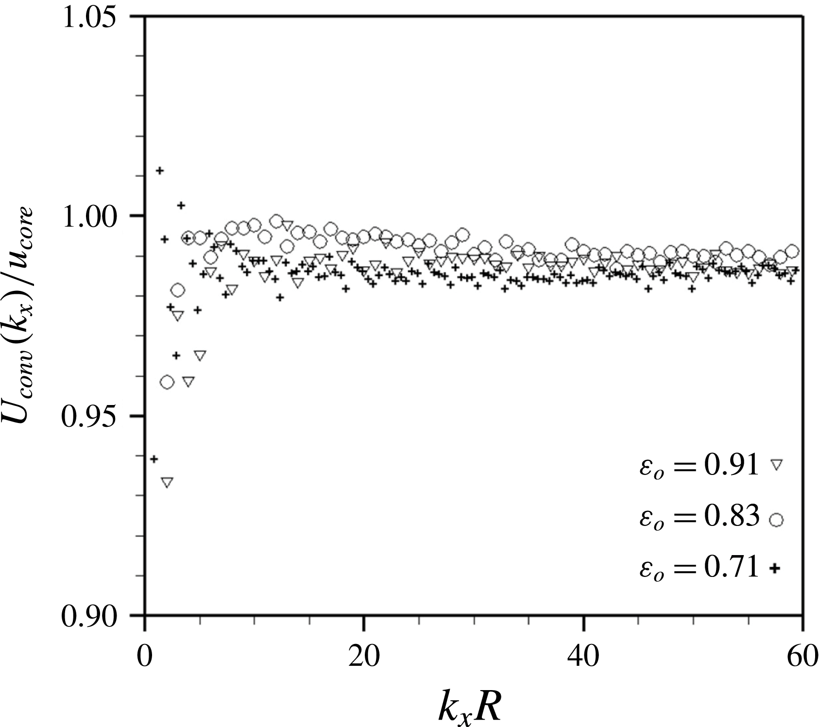
with the streamwise wavenumber. The scatter of the data shown in this figure is due to the limited statistical sample available for locating the maxima of the spectrum within a set of discrete frequencies and wavenumbers. The convection velocities at low wavenumbers are also contaminated by a specific window function (Hanning window) or a sampling period used (see Choi & Moin Reference Choi and Moin1990). The convection velocity increases with increasing
 $k_{x}$
, but maintains nearly a constant value
 $(=0.98{-}0.99u_{core})$
, slightly less than
 $u_{core}$
, at high wavenumbers. The overall convection velocity
 $U_{conv}$
of the most energetic wave is also obtained from
 $$\begin{eqnarray}\displaystyle & \displaystyle \left.{\displaystyle \frac{\unicode[STIX]{x2202}W(U^{\ast })}{\unicode[STIX]{x2202}U^{\ast }}}\right|_{U^{\ast }=U_{conv}}=0, & \displaystyle\end{eqnarray}$$
where
 $$\begin{eqnarray}\displaystyle & \displaystyle W(U^{\ast })=\int \unicode[STIX]{x1D6F7}(k_{x},-U^{\ast }k_{x})\,\text{d}k_{x}. & \displaystyle\end{eqnarray}$$
The overall convection velocities of the phase interface are calculated to be
 $U_{conv}/u_{core}=0.984,0.989,0.989,0.990$
and
 $0.985$
, respectively, for
 $\unicode[STIX]{x1D700}_{o}=0.91,0.83,0.71$
, 0.62 and
 $0.56$
, indicating that its most energetic motions travel downstream nearly at the core velocity.
Convection velocities as a function of the streamwise wavenumber.

3.3 Oil holdup model
The holdup is defined as the volume fraction of a particular fluid in a multiphase pipe flow. In experiments, the flow rates are controlled, but the holdups are not easily measurable. Thus, holdup models have been widely investigated (Oliemans Reference Oliemans1986; Bai et al. Reference Bai, Chen and Joseph1992; Arney et al. Reference Arney, Bai, Guevara, Joseph and Liu1993). In this study, we develop a new model to predict the oil holdup based on the observation that the flow in the annulus is divided by two characteristic regions: a boundary layer flow near the wall and a nearly constant velocity flow near and above the phase interface (see figure 7 b).
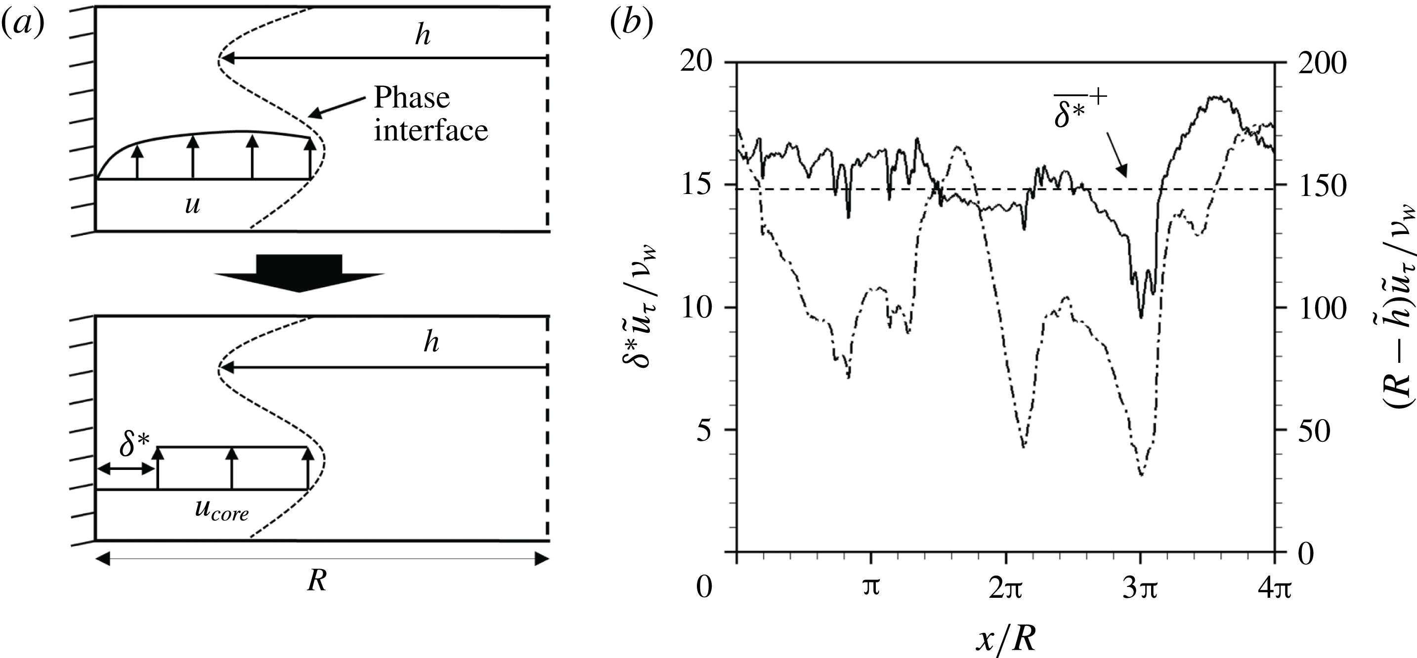
Displacement thickness
 $\unicode[STIX]{x1D6FF}^{\ast }$
(
 $\unicode[STIX]{x1D700}_{o}=0.71$
): (a) schematic diagram; (b) instantaneous streamwise distributions of the displacement thickness and
 $R-\tilde{h}$
in wall units with local friction velocity,
 $\tilde{u} _{\unicode[STIX]{x1D70F}}$
, at the same instant as in figure 4(b). In (b), ——,
 $\unicode[STIX]{x1D6FF}^{\ast }\tilde{u} _{\unicode[STIX]{x1D70F}}/\unicode[STIX]{x1D708}_{w}$
; – - – - –,
 $(R-\tilde{h})\tilde{u} _{\unicode[STIX]{x1D70F}}/\unicode[STIX]{x1D708}_{w}$
.

Since the flow field near the wall shows boundary layer characteristics except near the crest, we define a displacement thickness,
 $\unicode[STIX]{x1D6FF}^{\ast }(x,t)$
, as in figure 15(a), which satisfies
 $$\begin{eqnarray}\displaystyle & \displaystyle \int _{0}^{2\unicode[STIX]{x03C0}}\!\!\int _{h}^{R-\unicode[STIX]{x1D6FF}^{\ast }}u_{core}\,r\,\text{d}r\,\text{d}\unicode[STIX]{x1D703}=\int _{0}^{2\unicode[STIX]{x03C0}}\!\!\int _{h}^{R}u\,r\,\text{d}r\,\text{d}\unicode[STIX]{x1D703}. & \displaystyle\end{eqnarray}$$
By rearranging (3.12),
 $\unicode[STIX]{x1D6FF}^{\ast }(x,t)$
is given as
 $$\begin{eqnarray}\displaystyle & \displaystyle {\displaystyle \frac{\unicode[STIX]{x1D6FF}^{\ast }(x,t)}{R}}=1-\sqrt{1-{\displaystyle \frac{1}{\unicode[STIX]{x03C0}R^{2}}}\int _{0}^{2\unicode[STIX]{x03C0}}\!\!\int _{h}^{R}\left(1-{\displaystyle \frac{u}{u_{core}}}\right)\,r\,\text{d}r\,\text{d}\unicode[STIX]{x1D703}}. & \displaystyle\end{eqnarray}$$
Similarly, we define the overall displacement thickness
 $\overline{\unicode[STIX]{x1D6FF}^{\ast }}$
as (using (3.1) and (3.4))
 $$\begin{eqnarray}\displaystyle \displaystyle {\displaystyle \frac{\overline{\unicode[STIX]{x1D6FF}^{\ast }}}{R}} & = & \displaystyle 1-\sqrt{1-{\displaystyle \frac{1}{\unicode[STIX]{x03C0}R^{2}L_{x}T}}\int _{0}^{T}\!\!\int _{0}^{L_{x}}\!\!\int _{0}^{2\unicode[STIX]{x03C0}}\!\!\int _{h}^{R}\left(1-{\displaystyle \frac{u}{u_{core}}}\right)\,r\,\text{d}r\,\text{d}\unicode[STIX]{x1D703}\,\text{d}x\,\text{d}t}\nonumber\\ \displaystyle \displaystyle & = & \displaystyle 1-\sqrt{1-{\displaystyle \frac{1}{\unicode[STIX]{x03C0}R^{2}L_{x}T}}\int _{0}^{T}\!\!\int _{0}^{L_{x}}\!\!\int _{0}^{2\unicode[STIX]{x03C0}}\!\!\int _{0}^{R}\left(1-{\displaystyle \frac{u}{u_{core}}}\right)\unicode[STIX]{x1D713}\,r\,\text{d}r\,\text{d}\unicode[STIX]{x1D703}\,\text{d}x\,\text{d}t},\nonumber\\ \displaystyle \displaystyle & = & \displaystyle 1-\sqrt{1-{\displaystyle \frac{2}{R^{2}}}\int _{0}^{R}\left(\overline{\unicode[STIX]{x1D713}}-{\displaystyle \frac{\overline{u}_{w}^{\ast }}{u_{core}}}\right)\,r\,\text{d}r},\end{eqnarray}$$
where
 $T$
is the averaging time. Figure 15(b) shows the streamwise distribution of the instantaneous displacement thickness,
 $\unicode[STIX]{x1D6FF}^{\ast }\tilde{u} _{\unicode[STIX]{x1D70F}}/\unicode[STIX]{x1D708}_{w}$
, for
 $\unicode[STIX]{x1D700}_{o}=0.71$
, together with that of
 $(R-\tilde{h})\tilde{u} _{\unicode[STIX]{x1D70F}}/\unicode[STIX]{x1D708}_{w}$
, where
 $\tilde{h}=\int _{0}^{2\unicode[STIX]{x03C0}}h^{2}\,\text{d}\unicode[STIX]{x1D703}/\!\int _{0}^{2\unicode[STIX]{x03C0}}h\,\text{d}\unicode[STIX]{x1D703}$
and
 $\tilde{u} _{\unicode[STIX]{x1D70F}}=\sqrt{1/(2\unicode[STIX]{x03C0}\unicode[STIX]{x1D70C}_{w})\int _{0}^{2\unicode[STIX]{x03C0}}(-\unicode[STIX]{x1D707}\unicode[STIX]{x2202}u/\unicode[STIX]{x2202}r|_{wall})\,\text{d}\unicode[STIX]{x1D703}}$
(local friction velocity). The displacement thickness fluctuates around the overall displacement thickness, and its magnitude is much smaller than that of the averaged phase interface height except near the crest where
 $\unicode[STIX]{x1D6FF}^{\ast }\approx 0.4(R-\tilde{h})$
. The overall displacement thicknesses are
 $\overline{\unicode[STIX]{x1D6FF}^{\ast }}^{+}=\overline{\unicode[STIX]{x1D6FF}^{\ast }}u_{\unicode[STIX]{x1D70F}}/\unicode[STIX]{x1D708}_{w}\approx 6.98,14.85$
and
 $18.83$
for
 $\unicode[STIX]{x1D700}_{o}=0.91,0.71$
and
 $0.56$
in wall units, respectively, which increases with decreasing
 $\unicode[STIX]{x1D700}_{o}$
, but their magnitudes are small,
 $\overline{\unicode[STIX]{x1D6FF}^{\ast }}/R<0.027$
, indicating that most of water flows at
 $u_{core}$
. Equation (3.14) is rearranged using the superficial velocities and oil holdup
 $$\begin{eqnarray}\displaystyle & \displaystyle \unicode[STIX]{x1D700}_{o}=\left(1-{\displaystyle \frac{\overline{\unicode[STIX]{x1D6FF}^{\ast }}}{R}}\right)^{2}{\displaystyle \frac{1}{1+j_{w}/j_{o}}}. & \displaystyle\end{eqnarray}$$
Using (3.15), we confirmed that the overall displacement thicknesses of all experimental data in Vanegas Prada & Bannwart (Reference Vanegas Prada and Bannwart2001) are small,
 $\overline{\unicode[STIX]{x1D6FF}^{\ast }}^{+}<22$
. Note that the core velocity is nearly constant for
 $\unicode[STIX]{x1D700}\leqslant 0.71$
and that for
 $\unicode[STIX]{x1D700}=0.83$
is slightly smaller (see figure 10
a). This explains why the total volume flow rate for
 $\unicode[STIX]{x1D700}_{o}\leqslant 0.83$
in figure 3 is nearly constant.
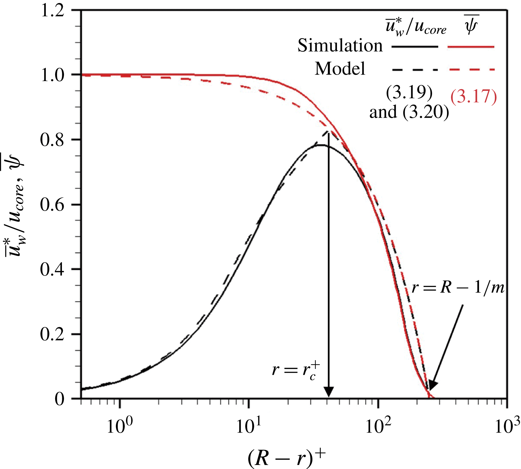
Profiles of the mean water volume fraction,
 $\overline{\unicode[STIX]{x1D713}}$
, and the mean streamwise velocity weighted by
 $\overline{\unicode[STIX]{x1D713}}$
,
 $\overline{u}_{w}^{\ast }$
, for
 $\unicode[STIX]{x1D700}_{o}=0.71$
.

To estimate the oil holdup, we need to approximate the overall displacement thickness
 $\overline{\unicode[STIX]{x1D6FF}^{\ast }}$
. Solid lines in figure 16 show the profiles of
 $\overline{u}_{w}^{\ast }/u_{core}$
and
 $\overline{\unicode[STIX]{x1D713}}$
obtained from the present simulation for
 $\unicode[STIX]{x1D700}_{o}=0.71$
. Two profiles collapse in the region of
 $\overline{u}_{w}\approx u_{core}$
because
 $\overline{u}_{w}^{\ast }=\overline{u}_{w}\overline{\unicode[STIX]{x1D713}}\approx u_{core}\overline{\unicode[STIX]{x1D713}}$
. Then, substituting (3.14) into (3.15) gives
 $$\begin{eqnarray}\displaystyle & \displaystyle \unicode[STIX]{x1D700}_{o}\approx \left\{1-{\displaystyle \frac{2}{R^{2}}}\int _{r_{c}}^{R}\left(\overline{\unicode[STIX]{x1D713}}-{\displaystyle \frac{\overline{u}_{w}^{\ast }}{u_{core}}}\right)\,r\,\text{d}r\right\}{\displaystyle \frac{1}{1+j_{w}/j_{o}}}, & \displaystyle\end{eqnarray}$$
where
 $r_{c}$
is defined such that
 $\overline{u}_{w}^{\ast }=\overline{\unicode[STIX]{x1D713}}u_{core}$
at
 $r\leqslant r_{c}$
. We model
 $\overline{\unicode[STIX]{x1D713}}$
as a linear profile whose slope is
 $m$
and magnitudes are 1 at
 $r=R$
and 0 at
 $r=R-1/m$
(figure 9):
 $$\begin{eqnarray}\displaystyle & \displaystyle \overline{\unicode[STIX]{x1D713}}=\left\{\begin{array}{@{}ll@{}}0\quad & \text{for }0\leqslant r<R-1/m,\\ 1-m(R-r)\quad & \text{for }R-1/m\leqslant r\leqslant R.\end{array}\right. & \displaystyle\end{eqnarray}$$
Here,
 $m$
is determined by matching the oil volume flow rate,
 $j_{o}\unicode[STIX]{x03C0}R^{2}=\int _{0}^{2\unicode[STIX]{x03C0}}\int _{0}^{R-1/m}$
 $u_{core}\,r\,\text{d}r\,\text{d}\unicode[STIX]{x1D703}+\int _{0}^{2\unicode[STIX]{x03C0}}\int _{R-1/m}^{R}u_{core}m(R-r)\,r\,\text{d}r\,\text{d}\unicode[STIX]{x1D703}$
:
 $$\begin{eqnarray}\displaystyle & \displaystyle m={\displaystyle \frac{2}{R(3-\sqrt{12\unicode[STIX]{x1D700}_{o}-3})}}, & \displaystyle\end{eqnarray}$$
where
 $12\unicode[STIX]{x1D700}_{o}-3\geqslant 0$
(i.e.
 $\unicode[STIX]{x1D700}_{o}\geqslant 1/4$
) is usually satisfied for the core-annular flow because the flow pattern changes for very low
 $\unicode[STIX]{x1D700}_{o}$
values (Bai et al.
Reference Bai, Chen and Joseph1992). For the integration in (3.16),
 $\overline{u}_{w}^{\ast }$
in
 $r_{c}\leqslant r\leqslant R$
is approximated with the mean velocity of the single-phase turbulent pipe flow (Spalding Reference Spalding1961) because of the high water fraction (
 $\overline{\unicode[STIX]{x1D713}}\approx 1$
):
 $$\begin{eqnarray}\displaystyle \displaystyle (R-r)^{+} & = & \displaystyle \overline{u}_{w}^{\ast +}+\exp (-\unicode[STIX]{x1D705}B)\left\{\exp (\unicode[STIX]{x1D705}\overline{u}_{w}^{\ast +})-1-\unicode[STIX]{x1D705}\overline{u}_{w}^{\ast +}-{\displaystyle \frac{(\unicode[STIX]{x1D705}\overline{u}_{w}^{\ast +})^{2}}{2}}-{\displaystyle \frac{(\unicode[STIX]{x1D705}\overline{u}_{w}^{\ast +})^{3}}{6}}\right\}\nonumber\\ \displaystyle & & \displaystyle \displaystyle \text{in }r_{c}\leqslant r\leqslant R,\end{eqnarray}$$
where
 $\unicode[STIX]{x1D705}=0.4$
,
 $B=5.5$
and
 $\overline{u}_{w}^{\ast +}=\overline{u}_{w}^{\ast }/u_{\unicode[STIX]{x1D70F}}$
. Also,
 $$\begin{eqnarray}\displaystyle & \displaystyle \overline{u}_{w}^{\ast }=u_{core}\overline{\unicode[STIX]{x1D713}}\quad \text{in }R-1/m\leqslant r\leqslant r_{c}. & \displaystyle\end{eqnarray}$$
The location
 $r_{c}$
is obtained by matching its velocity from (3.19) and (3.20). Finally, we adopt the friction factor model (Arney et al.
Reference Arney, Bai, Guevara, Joseph and Liu1993) to evaluate the wall friction:
 $$\begin{eqnarray}\displaystyle & \displaystyle \unicode[STIX]{x1D706}_{model}=\left({\displaystyle \frac{2\overline{\unicode[STIX]{x1D70F}}_{w}}{R}}\right){\displaystyle \frac{4R}{\unicode[STIX]{x1D70C}_{avg}(j_{o}+j_{w})^{2}}}=0.316Re_{model}^{-1/4}, & \displaystyle\end{eqnarray}$$
 $$\begin{eqnarray}\displaystyle & \displaystyle Re_{model}={\displaystyle \frac{2\unicode[STIX]{x1D70C}_{avg}(j_{o}+j_{w})R}{\unicode[STIX]{x1D707}_{w}}}\left\{1+\unicode[STIX]{x1D700}_{o}^{2}\left({\displaystyle \frac{\unicode[STIX]{x1D707}_{w}}{\unicode[STIX]{x1D707}_{o}}}-1\right)\right\}, & \displaystyle\end{eqnarray}$$
 $$\begin{eqnarray}\displaystyle & \displaystyle \unicode[STIX]{x1D70C}_{avg}=\unicode[STIX]{x1D70C}_{o}\unicode[STIX]{x1D700}_{o}+\unicode[STIX]{x1D70C}_{w}(1-\unicode[STIX]{x1D700}_{o}), & \displaystyle\end{eqnarray}$$
where
 $\unicode[STIX]{x1D706}_{model}$
is the friction factor of the turbulent core-annular flow. Given
 $j_{w}$
and
 $j_{o}$
, the oil holdup
 $\unicode[STIX]{x1D700}_{o}$
is obtained by iteratively solving (3.16)–(3.23). As shown in figure 16, the present model accurately predicts the velocity and water volume fraction.
Variation of the oil holdup with the superficial velocity ratio: (a)
 $\overline{\unicode[STIX]{x1D70F}}_{w}$
obtained from (3.21)–(3.23); (b)
 $\overline{\unicode[STIX]{x1D70F}}_{w}$
obtained directly from experimental data (Bai et al. (Reference Bai, Chen and Joseph1992) (
 $Re_{\unicode[STIX]{x1D70F}}\approx 100{-}350$
); Vanegas Prada & Bannwart (Reference Vanegas Prada and Bannwart2001) (
 $Re_{\unicode[STIX]{x1D70F}}\approx 600{-}1800$
)) and from present simulation (
 $Re_{\unicode[STIX]{x1D70F}}=720$
). Here, circles are the data from experiments, diamonds are from present numerical simulation, lines are from the previous models and present asymptotic solution and crosses are from the present model. The asymptotic solution is obtained with
 $\overline{\unicode[STIX]{x1D6FF}^{\ast }}=0$
(i.e. assuming that the bulk velocities of water and oil are same). Higher
 $\unicode[STIX]{x1D700}_{o}$
values than the asymptotic solution indicate that the bulk velocity of water is faster than that of oil because of an oil dispersion in water or oil adhesion to the wall (Vuong Reference Vuong2009). Our model does not consider this situation.

Figure 17 shows the predictions of the oil holdup from the present model for the previous experimental and present simulation data, together with the predictions from previous models and present asymptotic solution. Two predictions are shown in figures 17(a) and (b), respectively, based on the wall frictions from the present model (3.21)–(3.23) and from experimental data (Bai et al. Reference Bai, Chen and Joseph1992; Vanegas Prada & Bannwart Reference Vanegas Prada and Bannwart2001). The empirical correlations from previous studies and asymptotic solution are (original formulations are modified to compare with the present model)
 $$\begin{eqnarray}\displaystyle \displaystyle \unicode[STIX]{x1D700}_{o}=\left\{\begin{array}{@{}ll@{}}\left\{1-0.2{\displaystyle \frac{j_{w}}{j_{o}}}\left({\displaystyle \frac{1}{1+j_{w}/j_{o}}}\right)^{5}\right\}\left({\displaystyle \frac{1}{1+j_{w}/j_{o}}}\right)\quad & \text{(Oliemans 1986)},\\[13.0pt] \left({\displaystyle \frac{1+0.65j_{w}/j_{o}}{1+j_{w}/j_{o}}}\right)\left({\displaystyle \frac{1}{1+j_{w}/j_{o}}}\right)\quad & \text{(Arney et al. 1993)},\\[13.0pt] {\displaystyle \frac{1}{1+1.39j_{w}/j_{o}}}\quad & \text{(Bai et al. 1992)},\\[11.0pt] {\displaystyle \frac{1}{1+j_{w}/j_{o}}}\quad & \text{asymptotic solution}.\end{array}\right. & & \displaystyle\end{eqnarray}$$
Here, Oliemans (Reference Oliemans1986) suggested an empirical holdup model based on their experimental data from a horizontal core-annular flow, and Arney et al. (Reference Arney, Bai, Guevara, Joseph and Liu1993) modified it with more experimental data available in the literature. Bai et al. (Reference Bai, Chen and Joseph1992) also proposed an empirical holdup model for a vertical core-annular flow based on their experimental data. Note that the previous empirical holdup models obtained by fitting experimental data depend only on the superficial velocity ratio of oil to water and do not consider the Reynolds number dependence. As shown in this figure, the model of Bai et al. (Reference Bai, Chen and Joseph1992) well predicts their own experimental data, but not the data of Vanegas Prada & Bannwart (Reference Vanegas Prada and Bannwart2001). The present model considers not only the superficial velocity ratio but also the boundary layer characteristics of water flow representing the friction Reynolds number, and thus predicts both experimental data more accurately. The present model prediction in (b) is better than that in (a), indicating that the wall friction estimation is also important in estimating the oil holdup.
4 Conclusions
We investigated the characteristics of the core-annular flow of high viscosity oil and water using direct numerical simulation and level-set method for five different oil holdups (
 $\unicode[STIX]{x1D700}_{o}=0.56$
, 0.62, 0.71, 0.83 and 0.91) at a fixed mean wall friction (
 $Re_{\unicode[STIX]{x1D70F}}=720$
). The oil core flow was almost a plug flow and the water annular flow was a turbulent flow except for
 $\unicode[STIX]{x1D700}_{o}=0.91$
. The velocity profile of the core-annular flow was different from that of a single-phase turbulent pipe flow at a similar
 $Re_{\unicode[STIX]{x1D70F}}$
. The total volume flow rates for
 $\unicode[STIX]{x1D700}_{o}\leqslant 0.83$
were much higher than that of an oil pipe flow at the same
 $Re_{\unicode[STIX]{x1D70F}}$
and comparable to that of a water pipe flow. Therefore, as discussed in previous studies (Bai et al.
Reference Bai, Chen and Joseph1992; Vanegas Prada & Bannwart Reference Vanegas Prada and Bannwart2001), the core-annular flow was confirmed to be an effective tool to transport high viscosity oil. In the present study, the maximum oil flow rate occurred at
 $\unicode[STIX]{x1D700}_{o}=0.83$
. At higher
 $\unicode[STIX]{x1D700}_{o}$
, the oil flow rate decreased because the water region was so narrow that the core suffered from high wall shear stress.
The water flow was divided by two characteristic regions: a boundary layer flow near the wall and a nearly constant velocity flow near and above the phase interface (Bai et al.
Reference Bai, Kelkar and Joseph1996). The water near and above the phase interface moved almost with the core velocity but locally dragged oil downstream, although oil overall dragged water. Since the water flow near the wall was similar to a boundary layer flow, the displacement thickness was newly defined and was much smaller than that of the mean interface height from the pipe wall except near the crest. Vortical structures in the annular region existed at the locations ahead of the crests and in the valley regions, but little appeared behind the crests due to the small gap between the crest and wall. The pressures ahead of and behind the crests of the phase interface were high and low, respectively, because oil moved like a solid body at the speed of
 $u_{core}$
. The pressure in the valley region was more or less uniform. These pressure distributions agreed well with the results by RANS (Ko et al.
Reference Ko, Choi, Bai and Joseph2002; Ingen Housz et al.
Reference Ingen Housz, Ooms, Henkes, Pourquie, Kidess and Radhakrishnan2017).
The phase interfaces consisted of different streamwise and azimuthal wavenumber components for different oil holdups. As
 $\unicode[STIX]{x1D700}_{o}$
decreased, the PDF of the phase interface location became broader and moved towards the pipe centre. The instantaneous phase interface located near the wall had small wavelength and amplitude, but the one away from the wall had large wavelength and amplitude. The maximum radial locations of the phase interface was almost constant and very near the wall for different
 $\unicode[STIX]{x1D700}_{o}$
values, but the minimum location decreased with decreasing
 $\unicode[STIX]{x1D700}_{o}$
, indicating that the wave amplitude of the phase interface was larger at lower
 $\unicode[STIX]{x1D700}_{o}$
, which was in good agreements with the experimental results by Rodriguez & Bannwart (Reference Rodriguez and Bannwart2006). The power spectra of the phase interface amplitude were obtained as the function of the streamwise and spanwise wavenumbers and frequency. The spectra were broadbanded, indicating turbulent characteristics of the phase interface. The largest power occurred at the smallest azimuthal wavenumber whose corresponding wavelength was the pipe circumference. For the streamwise wavenumber spectra, more energy was concentrated on low wavenumbers with decreasing
 $\unicode[STIX]{x1D700}_{o}$
, which generated longer wavelength and large amplitude waves. The frequency spectra were similar to the streamwise wavenumber spectra due to the convective nature of the phase interface. The overall convection velocity of the phase interface was nearly the same as the core velocity.
Finally, we suggested a predictive model of the oil holdup considering the flow characteristics of the annular flow. This model predicted experimental and numerical data better than the previous predictive models. The applicability of the present model is limited when the phase interface is broken and oil bubbles form in water as in real situations (Bannwart et al. Reference Bannwart, Rodriguez, De Carvalho, Wang and Vara2004; Sotgia, Tartarini & Stalio Reference Sotgia, Tartarini and Stalio2008; Vuong Reference Vuong2009).
Acknowledgements
This work was supported by the NRF programs (NRF-2016R1E1A1A02921549 and NRF-2017M2A8A4018482) of MSIP and KETEP program (no. 20152020105600) of the MOTIE, Korea. The computer CPU time provided by the KISTI Supercomputing Center (KSC-2014-C2-044) is greatly appreciated.