1 Introduction
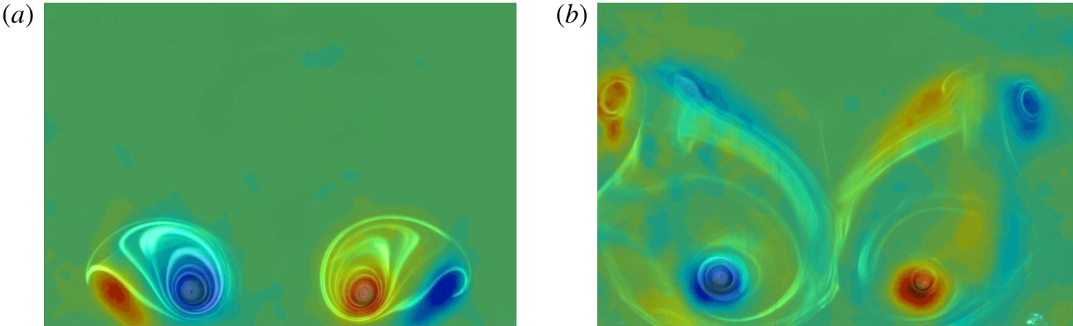
In this research, we study the impingement of a two-dimensional, counter-rotating vortex pair onto a wavy wall. For a vortex pair that is unstable to the long-wavelength Crow instability (Crow Reference Crow1970) interacting with a horizontal flat ground plane, the topology of the pair dramatically changes. This results in rebounding vortical structures, whose form is dependent on the extent of the instability prior to wall interaction (Asselin & Williamson Reference Asselin and Williamson2017). In this paper, by considering the complementary experiment of a straight vortex pair encountering a wavy wall, certain characteristics of the two flows are found to be similar. We find that the vortex pair first interacts with the ‘hills’ of the wall, leading to earlier generation of secondary vorticity in these regions and ultimately the formation of rising horizontal vortex rings.
Understanding vortex–wall interactions has applications in fundamental turbulence, in addition to practical applications. Vortical wall-bound structures such as horseshoe or hairpin vortices (streamwise vortex loops) can be found in turbulent boundary layers, and the presence of coherent vortices near a wall can give rise to offspring secondary vortices (Cantwell Reference Cantwell1981; Robinson Reference Robinson1991; Panton Reference Panton2001). Although seemingly simple, vortex pairs can produce complex three-dimensional dynamics due to instabilities or due to interactions with walls. The generation of counter-rotating vortices is also seen in the flow over submersible vehicles, such as submarines, wherein junction vortices are generated near appendages on the vehicle body. The rapid and quiet suppression of these vortices is important in improving the stealth capability of these vehicles (Quackenbush et al. Reference Quackenbush, Bilanin, Batcho, McKillip, Carpenter and Sater1997).
Vortex–ground interactions are also of particular interest in the context of aircraft trailing vortices, as is discussed extensively in the review by Spalart (Reference Spalart1998). Today, airports are required to handle an unprecedented number of air traffic take off and landings. An unavoidable by-product of lift is the generation of principal vortex structures taking the form of counter-rotating wing tip vortices. These vortices pose an increased hazard to following aircraft, as another aircraft flying through a vortex wake can experience dangerous rolling moments. The separation between the vortex cores,  $b_{0}$, and the circulation strength,
 $\unicode[STIX]{x1D6E4}$, are their dominant parameters, and the vortex pair can be observed as ‘contrails’ behind aircraft. A vortex pair can persist for long distances downstream of an aircraft. As such, one of the primary limiting factors in allowable traffic at airports is the time required for wing tip vortices to decay to safe levels. Such an aerodynamic hazard is even more dangerous near the ground, as there is often insufficient altitude for an aircraft to recover (Widnall Reference Widnall1975; Green Reference Green1995). In the past, Federal Aviation Administration (known as FAA) regulations have prescribed minimum separation distances based on aircraft weights and flying order, which increases safety but also increases airport delays (Green Reference Green1995; Spalart Reference Spalart1998). At present, wake turbulence recategorization (known as RECAT) regulations have been implemented at a number of airports to also take into account wingspan and aeroplane speed, allowing a decrease in minimum separation standards between aircraft. Alleviating the risk of wake vortices is of importance in both improving airline safety, and in increasing airport capacity.
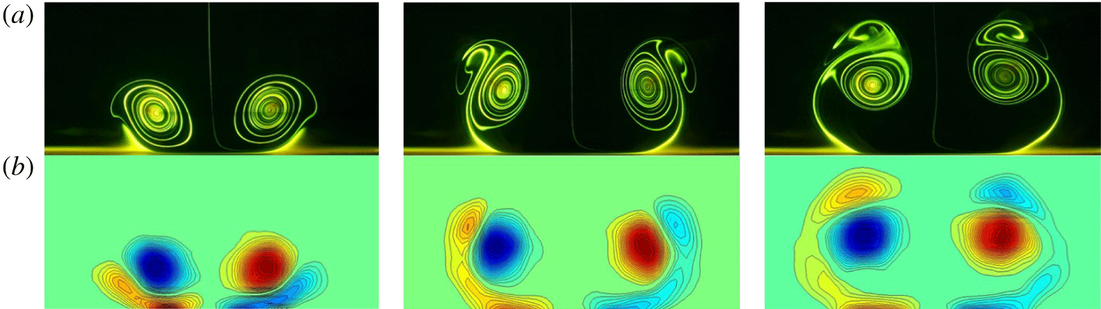
Flow visualization (a) and particle image velocimetry (b) showing a two-dimensional (straight) vortex pair interacting with the wall, and the development of secondary vorticity (Harris & Williamson Reference Harris and Williamson2012).

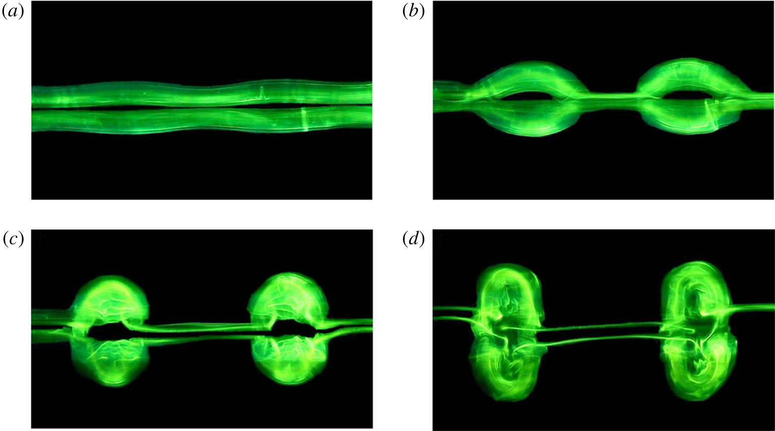
Development of the Crow instability in a vortex pair traveling towards the viewer. The initially straight vortex pair becomes sinusoidal in shape, before pinching off into vortex rings (Asselin & Williamson Reference Asselin and Williamson2017). See also Leweke & Williamson (Reference Leweke and Williamson2011).

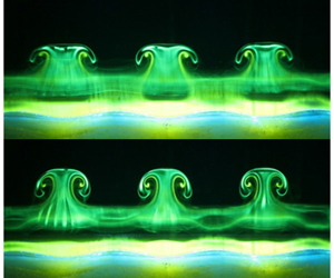
For an inviscid line vortex pair approaching a wall, Lamb (Reference Lamb1932) showed that the two vortices move away from each other along hyperbolic trajectories. However, for wake vortices behind aircraft, Dee & Nicholas (Reference Dee and Nicholas1968) observed that the vortex pair ‘rebounded’ away from the ground, rather than following this hyperbolic trajectory. Harvey & Perry (Reference Harvey and Perry1971) explained this rebound phenomenon as a result of the generation of secondary vorticity at the wall. When a vortex pair approaches a ground plane, a boundary layer forms between a vortex and the nearby wall boundary, that is subject to an adverse pressure gradient; this boundary layer can separate from the wall, generating a secondary vortex of opposite sign, and causing the primary pair to rebound. Figure 1 shows the roll up of opposite-signed secondary vorticity generated at the wall by Harris & Williamson (Reference Harris and Williamson2012), visualized both by laser induced fluorescence and particle image velocimetry (PIV). This rebound of the primary vortex at a wall was also observed by Barker & Crow (Reference Barker and Crow1977), and further analysed by Peace & Riley (Reference Peace and Riley1983).
Isolated vortex pairs, not in ground effect, can become unstable to short-wave (Widnall, Bliss & Tsai Reference Widnall, Bliss and Tsai1974) or long-wave instabilities (Crow Reference Crow1970). These instabilities are covered extensively in reviews by Widnall (Reference Widnall1975) and Leweke, LeDizès & Williamson (Reference Leweke, LeDizès and Williamson2016). The presence of instabilities in counter-rotating vortex pairs are particularly pertinent in aerodynamic applications, wherein natural instabilities can be exploited to hasten the breakdown of coherent vortices. The long-wave instability is of a bending displacement mode: the instability bends the cores of the primary vortices as a whole. Rather than decaying by diffusion, Crow (Reference Crow1970) observed that a counter-rotating vortex pair can undergo a symmetric, near-sinusoidal instability. Each vortex tube bends in a sinusoidal fashion in planes oriented at roughly  $45^{\circ }$ to the horizontal, growing in amplitude (see figure 2a,b). The curvature of the vortex leads to the two vortices being pushed together by their own self-induced velocity, such that they eventually reconnect, giving rise to a series of vortex rings as shown in figure 2(c,d) (see for example Leweke & Williamson (Reference Leweke and Williamson2011)). This has been observed both in the laboratory (Eliason, Gartshore & Parkinson Reference Eliason, Gartshore and Parkinson1975; Leweke & Williamson Reference Leweke and Williamson2011) and behind aircraft in the sky (Crow Reference Crow1970). Very good similarity exists between the full-scale phenomena and the phenomena in small-scale experiments, despite the difference in Reynolds number (
 $Re=O(10^{7})$ versus
 $Re=O(10^{3})$, respectively, see Leweke et al. (Reference Leweke, LeDizès and Williamson2016)). Following the formation of vortex rings, the vortex wake dissipates and poses less of a hazard (Chevalier Reference Chevalier1973).
In contrast, Widnall et al. (Reference Widnall, Bliss and Tsai1974) found that counter-rotating vortex pairs are also subject to a short-wave instability, that modifies the internal structure of the vortex cores rather than bending the entire vortex tube. This results in complex internal deformations in the vortex core. Leweke & Williamson (Reference Leweke and Williamson1998) experimentally investigated this elliptic instability, observing that the instabilities evolve in a ‘cooperative’ or coupled manner, exhibiting an antisymmetric, most unstable mode.
For a vortex pair in ground effect, the weaker secondary vortices that are generated at the ground are also subject to instabilities, resulting in three-dimensional flow structures arising from the initially two-dimensional vortex pair. The instability of the secondary vortex leads to coherent secondary loops that advect around the primary vortex. In the computational studies of both Luton & Ragab (Reference Luton and Ragab1997) and Duponcheel et al. (Reference Duponcheel, Cottin, Daeninck, Leweke and Winckelmans2007), it is suggested that this instability is of the short-wavelength elliptic instability type, particularly at high Reynolds numbers. For low-Reynolds-number cases, however, Harris & Williamson (Reference Harris and Williamson2012) find that the instability is of the displacement bending mode, such as is the Crow instability.
However, the selection of instability wavelength may be influenced initially by an elliptic instability (see discussion in Leweke et al. (Reference Leweke, LeDizès and Williamson2016) and Williamson et al. (Reference Williamson, Leweke, Asselin and Harris2014)). By keeping the primary vortices invisible in experiments, bending of the secondary vortex tubes can be observed: the instability perturbations of the two secondary vortices have an antisymmetric phase relationship across all experiments, suggesting a cooperative instability (Harris & Williamson Reference Harris and Williamson2012).
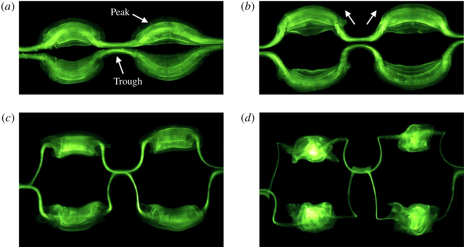
Flow visualization of the interaction of a vortex pair with Crow instability interacting with a wall, in ‘horizontal rings mode’. The vortex pair is moving towards the observer (Asselin & Williamson Reference Asselin and Williamson2017).

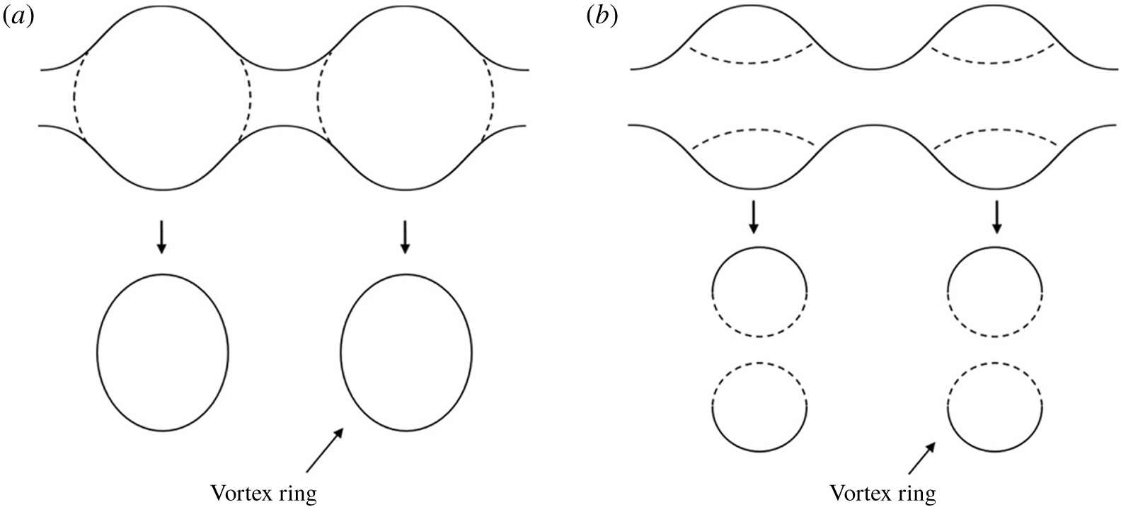
Comparison of the development of the Crow instability, (a) out of ground effect and (b) in ground effect. For the Crow instability out of ground effect, the two primary vortices pinch off to form one vortex ring per fundamental wavelength. For the Crow instability in ground effect, in ‘horizontal rings mode’ the primary and secondary vortices reconnect to form two vortex rings per fundamental wavelength.

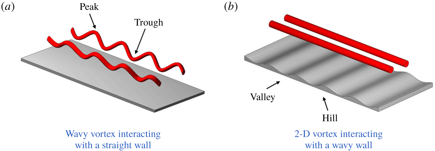
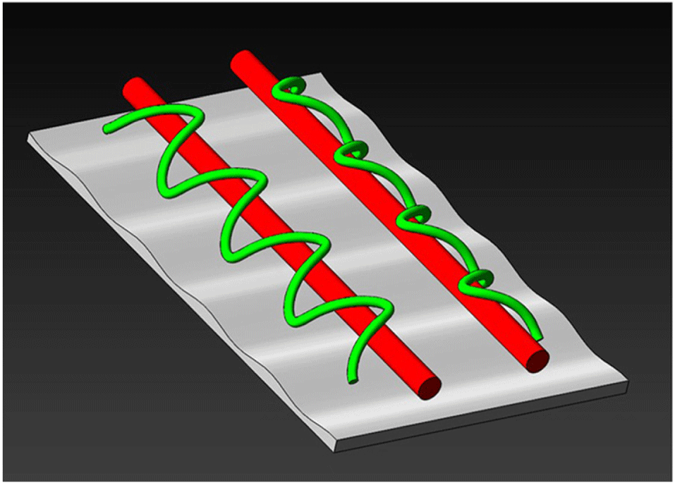
In contrast to a two-dimensional vortex pair, Asselin & Williamson (Reference Asselin and Williamson2017) conducted an extensive experimental study of a vortex pair with Crow instability interacting with a flat boundary. They found that upon interaction with the wall, the topology of the vortex pair changes, resulting in rebounding vortical structures whose form is dependent on the extent of the instability prior to wall interaction. For small initial heights, the Crow instability is inhibited, and the secondary vortices generated at the wall interact with each other to form ‘vertical rings’. At intermediate heights, the Crow instability is further developed such that the primary vortex pair has a distinct sinusoidal waviness, but still is inhibited from forming vortex rings (see figure 3). The ‘peak’ and ‘trough’ of the primary vortex are therefore at different heights above the ground plane. As a result, the ‘trough’ of the primary vortex will interact with the ground plane prior to the ‘peak’. A strong axial pressure gradient forms in the primary vortex, leading to axial flow in the primary vortex cores. In this mode, Asselin & Williamson (Reference Asselin and Williamson2017) observe that the primary and secondary vortices interact and form two rising horizontal rings: two per instability wavelength. This is called the ‘horizontal rings mode’. It is worth noting that these vortex rings are distinctly different from those observed by the Crow instability out of ground effect, which consist of only one ring per instability wavelength (see figure 4). It is suspected that given the complementary experiment of a straight vortex and a wavy wall, that one would see this same axial flow; this will be further discussed in § 4.
Due to the significant hazard trailing vortices pose to following aircraft, exploiting natural instabilities to alleviate the vortex wake hazard is an interesting avenue of research. The use of natural instabilities to mitigate this hazard can be broadly categorized into one of two methods, active or passive. Reviews of these methods can be found in Crouch (Reference Crouch2005) and Savaş (Reference Savaş2005).
Four-vortex systems consisting of two unequal-strength counter-rotating vortex pairs, such as is seen behind real aircraft with inboard flaps, are subject to both long-wavelength and short-wavelength instabilities (Crouch Reference Crouch1997). These unequal-strength vortices can be used to accelerate vortex decay out of ground effect by either actively or passively triggering instabilities in each pair. Active-controls systems such as periodic motions of control surfaces (Crouch, Miller & Spalart Reference Crouch, Miller and Spalart2001) or shape memory alloy (known as SMA) actuated devices (Quackenbush et al. Reference Quackenbush, Bilanin, Batcho, McKillip, Carpenter and Sater1997) force the early onset of these instabilities. In contrast, passive systems exploit natural instabilities. Rennich & Lele (Reference Rennich and Lele1999) show that for a four-vortex system, if the inboard flap can be configured to keep the inboard vortex in a region of high strain, perturbations on the vortex will grow rapidly to produce a Crow-like instability. Wings with triangular flap extensions were investigated by Ortega, Bristol & Savaş (Reference Ortega, Bristol and Savaş2002, Reference Ortega, Bristol and Savaş2003), producing counter-rotating vortex pairs consisting of both a flap vortex and tip vortex. The weaker flap vortex develops a rapidly growing sinusoidal displacement-type instability. The loops of the weaker vortex are brought together, and pinch off to yield a series of vortex rings.
(a) Schematic showing the Crow instability in ground effect as studied by Asselin & Williamson (Reference Asselin and Williamson2017). (b) The complementary experiment of a two-dimensional (straight) vortex pair impinging on a wavy wall.

Another method of wake hazard alleviation is to use a ground-based approach. The application of blowing or suction of air at the wall is shown to increase the lateral displacement of the vortex pair at the ground (Wakim et al. Reference Wakim, Brion, Dolfi-Bouteyre and Jacquin2020). The use of a passive, ground-based approach has been explored by the German Aerospace Center (DLR - Deutsches Zentrum für Luft-und Raumfahrt). By modifying the ground plane, the secondary vortex structures that form upon vortex–wall interaction can be manipulated to accelerate the decay of the primary vortex pair. Stephan, Holzäpfel & Misaka (Reference Stephan, Holzäpfel and Misaka2013a) and Stephan et al. (Reference Stephan, Holzäpfel, Misaka, Geisler and Konrath2013b) investigate by large eddy simulation and experiment (towing tank) the interaction of a counter-rotating vortex pair with a wall, whereupon sits a large rectangular (cuboidal) obstacle. This obstacle is placed perpendicular to the length of the vortices, such that it transects both vortex cores. Interaction with the obstacle triggers the formation of secondary vortex structures, as secondary vorticity is initiated earlier at the top of the obstacle. These secondary vortex structures detach and take the form of a distinct  $\unicode[STIX]{x1D6FA}$-shaped loop. This
 $\unicode[STIX]{x1D6FA}$-shaped secondary vortex travels along the primary vortex by self-induction. The interaction of primary and secondary vorticity substantially accelerates the decay of the primary vortex in comparison to a wall with no obstacle.
Other studies of vortex pairs impinging on perturbed surfaces also show an accelerated rate of circulation decay. Both rough (rectangular-shaped perturbations, parallel to the vortex pair) and water surfaces lead to an increase in the rate of vortex circulation decay (Zheng & Wei Reference Zheng and Wei2013; Kazarin & Golubev Reference Kazarin and Golubev2017). The use of ground-based obstacles to modify vortex–ground interactions is an effective means of alleviating the wake vortex hazard at low altitudes near the ground plane.
In this paper, we observe that the impingement of a straight vortex pair onto a wavy wall manipulates the shape of the secondary vorticity generated at the wall, and leads to an accelerated decay of the primary vortex pair. This is consistent with previous observations by Stephan et al. (Reference Stephan, Holzäpfel, Misaka, Geisler and Konrath2013b), wherein the stretching of the secondary vortex in the flow field of the primary vortex pair is associated with a decrease in circulation of the primary vortices. The circulation within the primary vortex decays on account of the primary vortex interacting with on the secondary vortex structure.
The breakup of trailing vortices is desirable in a practical sense, as we aim to diminish the wake vortex hazard posed by aircraft in their lines of approach and departure to and from airports. This study forms the complimentary experiment to a vortex pair with Crow instability impinging on a flat wall (see figure 5). It is expected that similar flow features, such as the formation of small-scale vortex rings, will be observed in the case of a straight vortex pair interacting with a wavy wall. We present experimental methods in § 2, followed by a discussion in § 3 of the dominant flow features observed both by flow visualization and particle image velocimetry. The formation of geometrically influenced secondary vortex loops as a result of the primary vortex pair interacting with the wall at different times is presented, as well the pinching off of these vortex loops into rising horizontal vortex rings (two per fundamental wavelength). In § 4 we discuss the three main results arising from this study. Firstly, we present evidence showing the formation of these rising horizontal vortex rings using flow visualization and particle image velocimetry in conjunction with one another. Following this, we discuss the accelerated decay of the primary vortex pair as a result of the perturbed ground plane. It is shown that the addition of significant ground-based obstacles at the wall is a conceivable means of reducing the wake vortex hazard near the ground. Lastly, we are presented with an unanticipated result. As the topological changes observed in the complementary experiment by Asselin & Williamson (Reference Asselin and Williamson2017) are primarily driven by large axial flows in the primary vortex core, we expected to see significant axial flow in the primary vortices in the present study. It is surprising that we establish a lack of axial flow in the studied wavy wall configuration, as the small-scale vortex structures that are produced from this flow originate solely from secondary vorticity. In § 5 we discuss the effects of varying the hillock parameters (amplitude and wavelength), and in § 6 we present practical applications of this work. Conclusions follow in § 7.
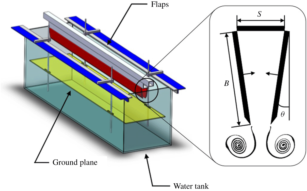
Schematic of the vortex generator facility, showing the adjustable ground plane and flaps. Here,  $\unicode[STIX]{x1D6E9}$ is the angle of flap rotation,
 $B$ is the length of the flaps and
 $S$ is the distance separating the base of the flaps (Asselin & Williamson Reference Asselin and Williamson2017).

2 Experimental details
Experiments were conducted using the Cornell University Fluid Dynamics Research Laboratories’ vortex generator facility. Originally constructed by Thomas Leweke (for details see Leweke & Williamson (Reference Leweke and Williamson1998, Reference Leweke and Williamson2011)), the facility has since undergone modifications to increase reliability and repeatability.
The vortex generator facility consists of a glass-walled, rectangular tank, measuring  $180~\text{cm}\times 45~\text{cm}\times 60~\text{cm}$. Two anodized aluminium flaps are hinged at a common rectangular base, and are closed simultaneously by use of computer-controlled stepper motors. The base and flaps are lowered into the tank by a second set of computer-controlled stepper motors (see figure 6). The flaps measure
 $170~\text{cm}$, extending nearly the entire length of the tank. The ends of the flaps are designed such that end effects are minimized (Leweke & Williamson Reference Leweke and Williamson1998).
The vortex generator facility also includes a transparent, horizontal acrylic ground plane submerged in the tank. It is removable and adjustable, with its position secured by manual lead screws. The initial height of the flaps above the ground is given by  $h_{0}$, and is set to
 $10~\text{cm}$ for each experiment. We first detect secondary vorticity in our PIV when the primary vortex pair is
 ${\approx}1.25b_{0}$ above the wall. Vortices are generated far enough above the ground plane that the presence of the wall does not inhibit vortex formation (Fogg Reference Fogg2001). The width of the tank is equivalent to
 $22.5b_{0}$, and so does not hinder any transverse vortex motion. We also ensure that instabilities do not develop along the length of the vortex pair prior to ground interaction.
The vortex pair impinges upon a wavy wall which is placed upon the horizontal ground plane. Opaque hillocks are rapidly prototyped using an Objet30 3-D printer, using either Objet VeroWhitePlus or VeroBlue resin. This allows us to produce hillocks of varying amplitudes and wavelengths; throughout this paper, unless otherwise stated, the hillock has an amplitude,  $A$, of
 $0.2~\text{cm}$ and spanwise wavelength,
 $\unicode[STIX]{x1D706}$, of
 $6~\text{cm}$. Rather than trying to trigger a Crow-type instability at the wall, this configuration was chosen due to its consistency in producing coherent secondary vortex structures. When VeroWhitePlus resin is used, the hillock is coated in spray epoxy to reduce water absorption, followed by matt black spray paint to reduce reflections in imaging. Results for varying
 $A$ and
 $\unicode[STIX]{x1D706}$ can be found in § 5.
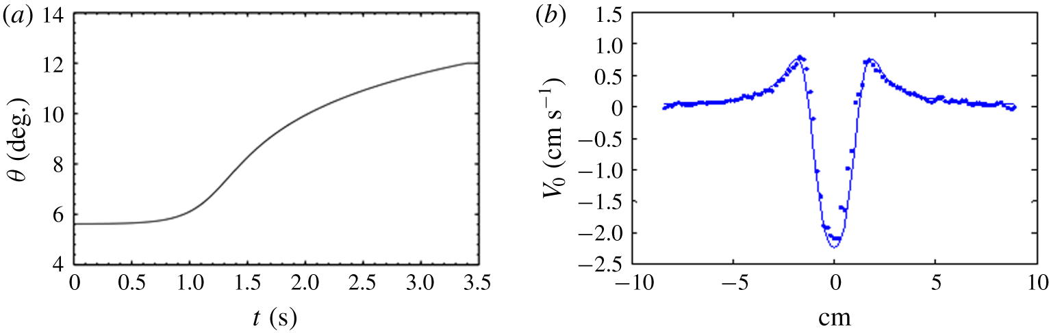
(a) Motion profile developed by Leweke & Williamson (Reference Leweke and Williamson2011) for closing the flaps to generate Gaussian vortices. The angle of flap rotation,  $\unicode[STIX]{x1D6E9}$, is shown against time,
 $t$. (b) A least squares best fit of the superposition of two Lamb–Oseen vortices to the measured azimuthal velocity profile, measured from particle image velocimetry.

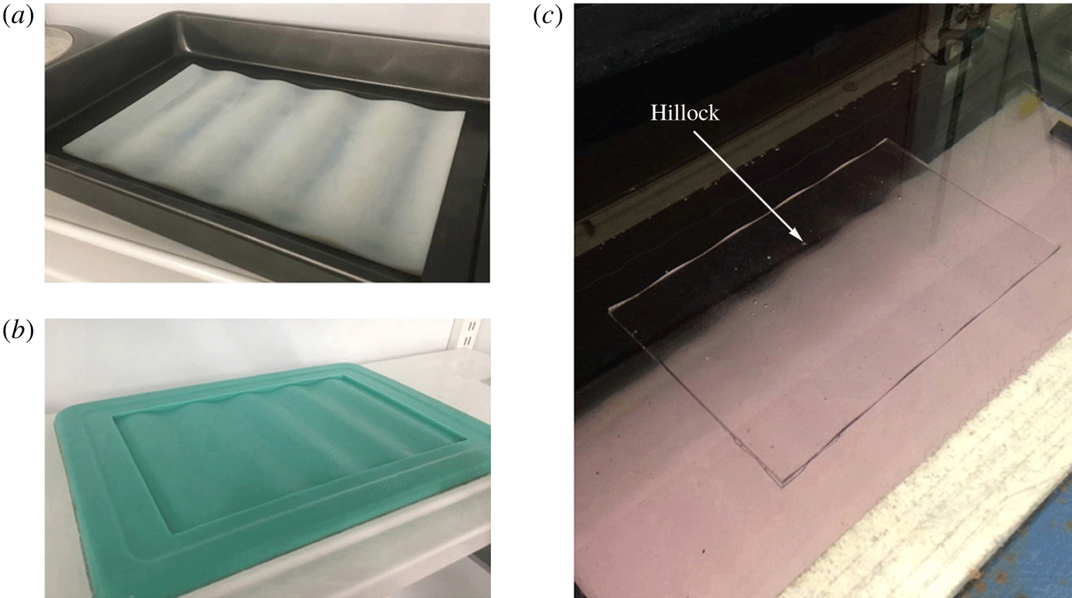
(a) Three-dimensional printed positive hillock, in a tray to make the mould. (b) Negative silicon mould made from Smooth-on Mold Star 15 Slow. (c) Final transparent hillock submerged in water on the ground plane, made from Smooth-on Crystal Clear 200 acrylic resin.

The counter-rotating vortex pair that impinges on the hillocks is produced by closing the computer-controlled flaps. When the flaps are closed, fluid is displaced vertically downward, and shear layers from the flaps roll up into coherent vortices. The motion profile of the edge of the plates was determined empirically by Leweke & Williamson (Reference Leweke and Williamson2011) to produce a two-dimensional laminar vortex pair. As shown in figure 7, the vertical (azimuthal) velocity of this vortex pair is well modelled by the superposition of two Lamb–Oseen (Gaussian) vortices. The azimuthal velocity profile of each Lamb–Oseen vortex is
 $$\begin{eqnarray}v_{\unicode[STIX]{x1D703}}(r)=\frac{\unicode[STIX]{x1D6E4}}{2\unicode[STIX]{x03C0}r}\left[1-\exp \left(\frac{-r^{2}}{a^{2}}\right)\right],\end{eqnarray}$$
where  $\unicode[STIX]{x1D6E4}$ is the circulation of the vortex,
 $r$ is the distance measured from the vortex centre, and
 $a$ is a parameter characterizing the core size of the vortex.
Transparent hillocks are custom cast with Smooth-On Crystal Clear 200 acrylic resin, as described by Bristow et al. (Reference Bristow, Blois, Kim, Best and Christensen2016). An opaque 3-D printed positive of the hillock is used to create the negative mould in a tray, using Smooth-On Mold Star 15 Slow silicone rubber. By polishing the printed positive beforehand, the mould is smooth enough to negate the need for further polishing after casting. Crystal Clear 200 acrylic resin is used to make the transparent casting, due to its optical clarity (see figure 8c). Once in the mould, the resin is placed in a pressure pot to reduce bubble defects, and heat cured using the facilities in Professor Robert Shepherd’s Organic Robotics Laboratory at Cornell University. The final product allows us to pass a laser sheet through the hillock for imaging directly above the hillock.
Two different techniques are used to analyse the flow: laser-induced fluorescence dye visualization, and PIV. For flow visualization, fluorescein dye is illuminated by a 5-W Coherent Innova 70 argon-ion laser. The flow can either be floodlit for a view of the entire flow by passing the laser through a plano-convex lens, or a particular cross-section can be illuminated by using a cylindrical lens. A key feature of this experiment is the ability to visualize the primary and secondary vortices either independently or concurrently. The primary vortex pair is made visible by directly painting the flaps with a mixture of fluorescein dye and water. In contrast, the dye is carefully pooled (prior to the experiment) on the surface of the hillocks to visualize the secondary vortices, as described in Harris & Williamson (Reference Harris and Williamson2012). Images are acquired using computer-controlled digital single lens reflex (DSLR) cameras at a rate of 1 Hz. We can use two cameras at different positions to simultaneously capture the flow from different viewpoints.
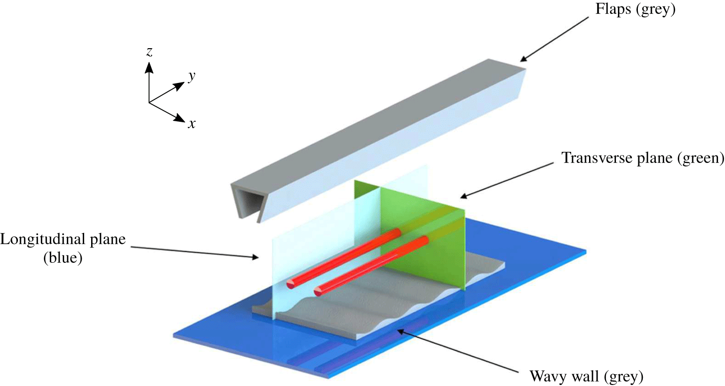
Schematic of the two principal planes studied. The transverse plane cuts the core of the vortex pair (red), and the longitudinal plane extends the length of the hillock.

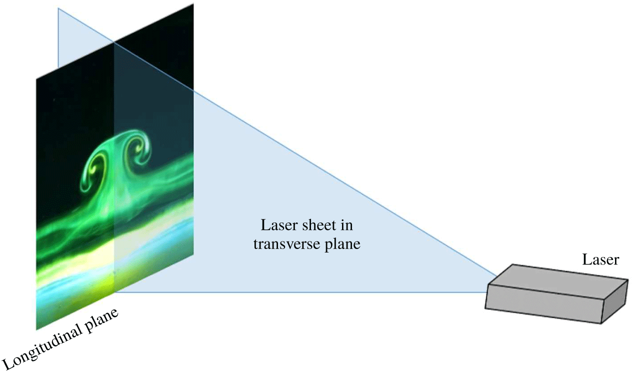
Schematic showing the set-up of a laser light sheet for PIV of the transverse plane.

Particle image velocimetry is used to obtain quantitative measurements of the flow. Prior to experiments, the tank is seeded with particles (Potters’ Industries Sphericel 110P8, mean diameter  $10~\unicode[STIX]{x03BC}\text{m}$ and density
 $1.10~\text{g}~\text{cm}^{-3}$). A 5 W argon-ion laser is again used with a cylindrical lens to illuminate planes of the flow. Figure 9 shows the different cross-sectional planes used throughout the study; figure 10 shows an example of a transverse light sheet through the middle of a hillock valley. A charge-coupled device (known as CCD) Kodak MegaPlus 1 megapixel digital camera is used to capture images, at a rate of 15 Hz. Velocity fields are then calculated by processing pairs of these images using PIVLab software (Thielicke Reference Thielicke2014; Thielicke & Stamhuis Reference Thielicke and Stamhuis2014a,Reference Thielicke and Stamhuisb). Using these PIV measurements, the velocity fields are further processed to determine initial conditions of the flow, and other parameters of interest.
The vortex position is measured by tracking the location of maximum vorticity over time. These measurements give us the initial vortex spacing,  $b_{0}$. Using the vorticity field, vorticity contours are obtained for each frame. Circulation of the vortex is calculated by taking the line integral of the velocity field around a contour matching 5 % of the maximum measured vorticity in the vortex. From this data, we obtain the initial circulation,
 $\unicode[STIX]{x1D6E4}_{0}$. The circulation-based Reynolds number is therefore
 $$\begin{eqnarray}Re=\frac{\unicode[STIX]{x1D6E4}_{0}}{\unicode[STIX]{x1D708}},\end{eqnarray}$$
where  $\unicode[STIX]{x1D708}$ is the kinematic viscosity of water. In all experiments,
 $Re\approx 800$, and the ratio of initial core size to initial vortex spacing,
 $a_{0}/b_{0}\approx 0.4$; the initial vortex spacing
 $b_{0}=2~\text{cm}$. The ratio of the initial vortex spacing to height of vortex generation,
 $b_{0}/h_{0}=0.2$. The dimensions of the hillock expressed in terms of
 $b_{0}$ are
 $A/b_{0}=0.1$ and
 $\unicode[STIX]{x1D706}/b_{0}=3$. Time is non-dimensionalized by the time required for the vortex pair to descend a distance equal to one initial vortex spacing, with time starting from the first motion of the flaps; this is given by
 $$\begin{eqnarray}t^{\ast }=t\frac{\unicode[STIX]{x1D6E4}_{0}}{2\unicode[STIX]{x03C0}b_{0}^{2}}.\end{eqnarray}$$
Multiple experiments were run in order to characterize the uncertainty of the measured initial conditions. The 95 % confidence interval for the value of  $\unicode[STIX]{x1D6E4}_{0}$ is
 $\pm 2.9\,\%$. The uncertainty for
 $b_{0}$ is
 $\pm 4.5\,\%$, and the variation in vortex core size is
 $\pm 1.2\,\%$.
3 Dominant flow features of a vortex pair interacting with a wavy wall
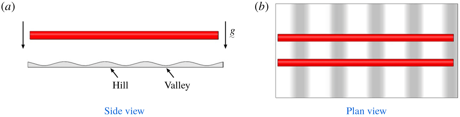
In this section, we shall show the essential flow features that arise when a two-dimensional vortex pair interacts with a wavy wall. It is expected that we will observe topological changes of the vortex pair and rebounding vortical structures. We show that the descending two-dimensional (2-D) vortex pair first interacts with the hills of the wall on the ground plane, resulting in earlier localized secondary vorticity generation than is found for the valleys. This leads to the formation of secondary vortex loops in the valleys, which pinch off into rising vortex rings, two per fundamental wavelength. The location of the hills and valleys can be seen in figure 11.
(a) Side view of the primary vortex pair impinging on the hillock. (b) Plan view of the primary vortex pair impinging on the hillock.

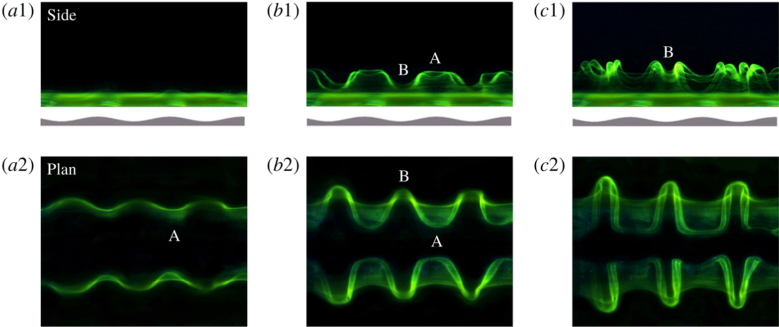
Flow visualization of the development of secondary vorticity. Side view (a1,b1,c1) and plan view (a2,b2,c2) images are taken simultaneously. The letter ‘A’ marks the location over the hill where secondary vorticity is first generated, and ‘B’ marks the location in the valley where the secondary loop forms. (a1,a2) are at  $t^{\ast }=4.6$, (b1) and (b2) at
 $t^{\ast }=5.2$, and (c1,c2) at
 $t^{\ast }=5.8$.

Flow visualization is initially employed to see the large-scale features of the flow. To accurately define the vortex structures, both flow visualization and PIV is required, as the rate of diffusion of dye is different to that of vorticity. The DSLR cameras are placed both below and at the side of the vortex generator tank to simultaneously take plan view and side view images of the vortex pair, as shown in figure 11. End view images are taken by imaging the transverse plane, shown in figure 9.
3.1 Primary and secondary flow visualization
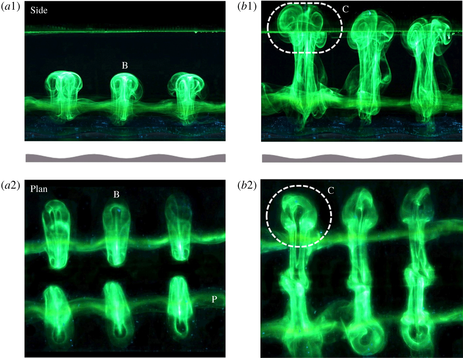
Figure 12 shows the evolution of secondary vorticity in side view and plan view by carefully pooling dye on the wavy wall and using a floodlit laser. By keeping the primary vortices invisible, we track the motion of just the secondary vorticity. The key to the three-dimensional (3-D) vortex dynamics is the fact that the primary vorticity travelling vertically downwards comes into proximity with the wavy wall along the hill first, then the valley. The secondary vorticity rolls up and is advected around the primary vortex earlier, in the vicinity of the hill at point ‘A’. This is seen in figures 12(a1,a2) and 12(b1,b2). As the secondary vortex over the hill is advected around the primary vortex and descends, the secondary vortex tube forms a vortex loop along the valley at point ‘B’. A series of secondary vortex loops form in the valleys, two per fundamental wavelength. This is seen in figures 12(b1,b2) and 12(c1,c2). The self-induction of the vortex loop on itself causes the vortex loop to rise vertically upward.
Primary flow visualization, wherein the development of both primary and secondary vorticity can be seen. Side view (a1,b1) and plan view (a2,b2) images are taken simultaneously. The letter ‘B’ marks the location in the valley where the secondary loop forms, and ‘C’ shows the formation of vortex rings, two per fundamental wavelength. (a1,a2) are at  $t^{\ast }=7.0$, and (b1,b2) at
 $t^{\ast }=12.8$. The letter ‘P’ shows the position of the primary vortex. The green line in (a1,b1) indicates dye at the edge of the flaps.

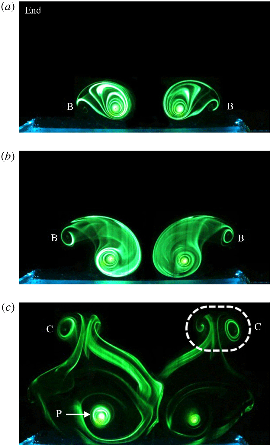
Transverse cross-section of primary flow visualization. Panels (a–c) are taken at  $t^{\ast }=5.8,7.0,$ and
 $15.1$, respectively. The letter ‘B’ marks the location in the valley where the secondary loop forms, and ‘C’ shows the formation of a vortex ring, two per fundamental wavelength. Here, ‘C’ is equivalent to the vortex rings observed in figure 13(b2). The letter ‘P’ shows the position of the primary vortex.

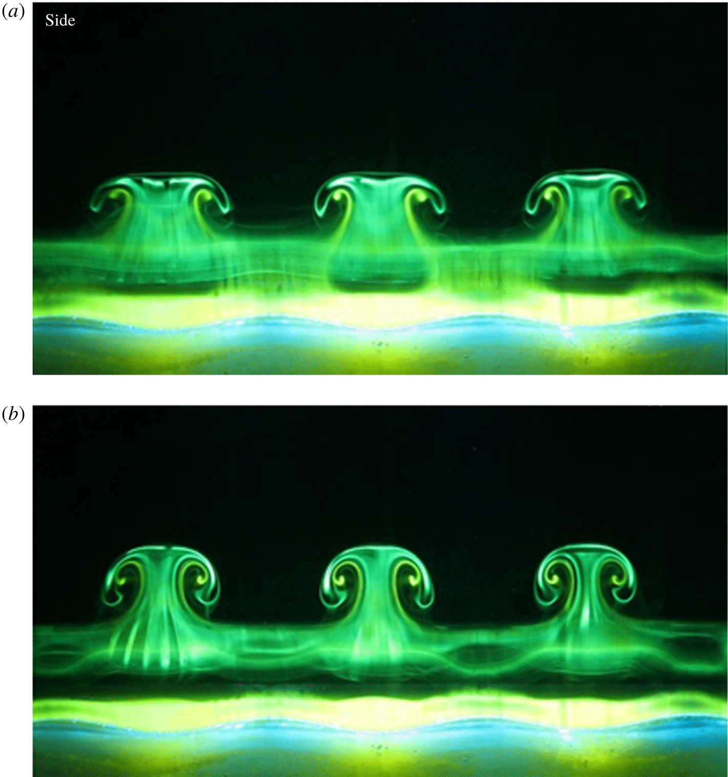
We again observe the formation of vortex loops in the valleys by floodlit primary flow visualization in figure 13. The sequence of images in figure 13 occur at a later time than in figure 12. In this case, the flaps of the vortex generator facility are painted with dye, making the primary vortex pair visible. Although the dye originally marks the primary vortices, the dye also makes visible the secondary vortex structure following interaction with the wall. The primary vortices remain visible as the straight line of dye across each image in figure 13. Figure 13(a1,a2) again shows the formation of secondary vortex loops at point ‘B’ in the valleys. The vortex loops rise vertically upward under their own self-induction, having already risen much higher than the primary vortex rebound height. In figure 13(b2), the bottom of the secondary vortex loops in the valley approach each other between the primary vortices. The ‘knot-like’ structure in the centre of this figure shows this region of interaction; however, the physics at this location are unclear from dye visualization. Ultimately, a vortex ring is formed near the end of the vortex loop by a pinching off process, marked as point ‘C’. These vortex rings, two per fundamental wavelength, also rise vertically upward due to their own self-induction. Due to the difference in diffusion rates of dye and vorticity, PIV is required to confirm the presence of these vortex rings. This will be shown in § 4.
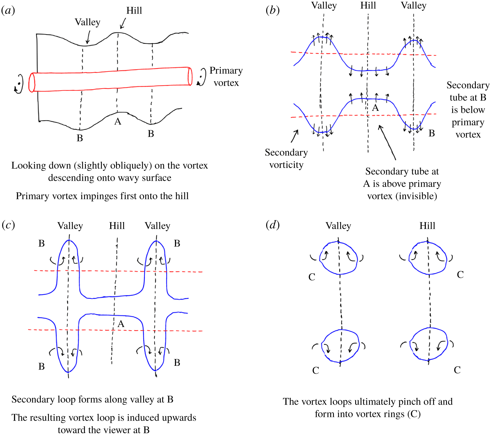
Schematic of the key vortex dynamics that lead to the generation of secondary vortex rings. Secondary vorticity is indicated by blue, primary vorticity is indicated by red.

In addition to floodlit flow visualizations, 2-D cross-sectional images show the development of the secondary vortex structure. Figure 14 shows a transverse cut of the flow through the middle of a valley, as described in figure 9. Point ‘B’ in the valley shows the roll up of the opposite-signed secondary vortex. The vortex loop that is formed in the valley rises vertically upward in figure 14(a,b). By figure 14 (c), a vortex ring has formed, shown by point ‘C’. In this image, the dye has spread around the entire vortex ring. It is also noteworthy that the primary vortex core remains intact and visible. As the secondary vortex structure becomes highly three-dimensional, the primary vortex core remains in the same location.
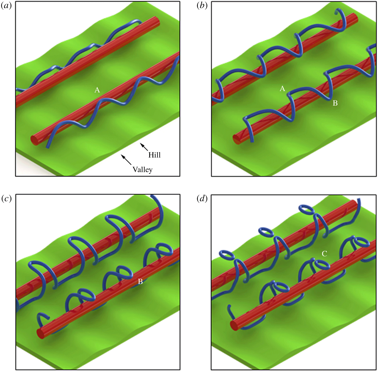
Figure 15 shows a schematic of the key vortex dynamics that lead to the generation of secondary vortex rings. As discussed earlier, the primary vortex impinges first onto the hill at ‘A’. A secondary vortex loop forms along each valley at ‘B’, and the resulting self-induced motion of the vortex loop is upward away from the wavy wall. The vortex loops pinch off and form into vortex rings, indicated by point ‘C’.
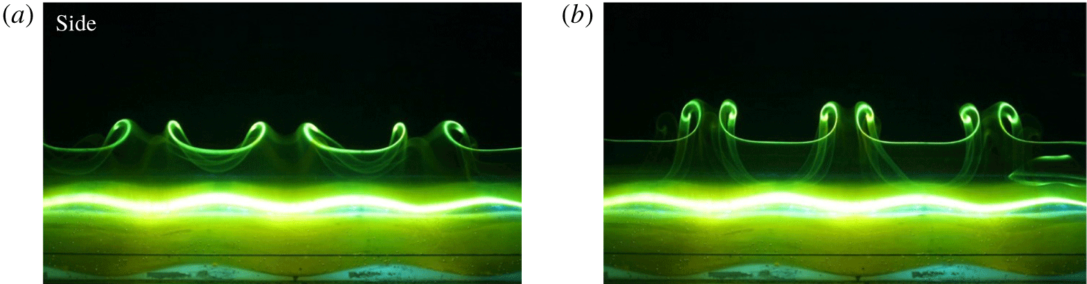
Longitudinal cross-section of secondary flow visualization, across three wavelengths. Panels (a–b) are taken at  $t^{\ast }=6.4$ and
 $7.0$, respectively.

Longitudinal cross-section of simultaneous primary and secondary flow visualization, across three wavelengths. Panels (a–b) are taken at  $t^{\ast }=6.4$ and
 $7.0$, respectively (Morris & Williamson Reference Morris and Williamson2017).

We also take longitudinal cross-sectional images to see the formation of the secondary vortex structures across multiple wavelengths. Figure 16 shows only secondary vorticity, whereas figure 17 uses both primary and secondary flow visualization simultaneously. The secondary dye (lighter green) is ‘nested’ within the primary dye (darker green). The formation of secondary vortex loops above each valley is observed in both figures 16 and 17. The primary vortex is once again observed horizontally across both images in figure 17, as the secondary vortex structures rise vertically upward.
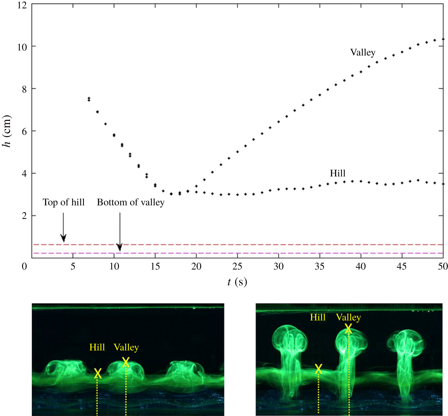
The height position of the primary and secondary vorticity is shown in figure 18. We track the position (marked as a yellow X) of the top of the primary vortex over the hill, and the top of the secondary vorticity in the valley. Following wall interaction, the primary vortex rests at a single location. In contrast, the secondary vortex structures rise upward at a comparable ascent velocity to the initial descent velocity ( ${\approx}0.6u_{descent}$) due to their own self-induction.
Plot of height of the vortex above the ground against time, for different locations. The primary vortex is tracked over the hill, whereas the secondary vortex structure is tracked by the top of the rising vortex rings. These are marked by a yellow ‘X’ in the flow visualization.

Using the flow visualization images and our schematic, a series of computer-generated schematics were assembled using SolidWorks. Matching  $x$-,
 $y$- and
 $z$-coordinates of the secondary vortex from simultaneous side view and plan view images allowed us to render a 3-D representation of the shape of the secondary vortex loops; this is discussed further in appendix A. A parametric solution was used to describe the resultant 3-D shape, with the plan view represented by a sine curve and the side view represented by a second-order Fourier series. Inspired by this and using the information gathered from figures 12–17, we generated a series of schematics, showing the development of the secondary vortex. Note that these images are a visual representation of the three-dimensional flow structures observed.
SolidWorks rendition of the development of the secondary vortex structure. (a) The initial development of secondary vorticity over the hills is marked as ‘A’. (b) The secondary vorticity generated at ‘A’ advects around the primary vortex, as the secondary vorticity in the valley, marked as ‘B’, is generated. (c) The secondary vortex tube forms a rising vortex loop ‘B’ in the valley. (d) The vortex loop pinches off into a vortex ring, ‘C’, two per fundamental wavelength. These vortex rings continue to rise upward by their own self-induction.

The development of the secondary vorticity is represented by the blue vortex tube in figure 19. Corresponding with our results in figures 12 and 13 earlier, we observe the formation of vortex loops and vortex rings due to the dynamics of the secondary vortices in the presence of the wavy wall.
3.2 Primary and secondary vorticity measurements using PIV
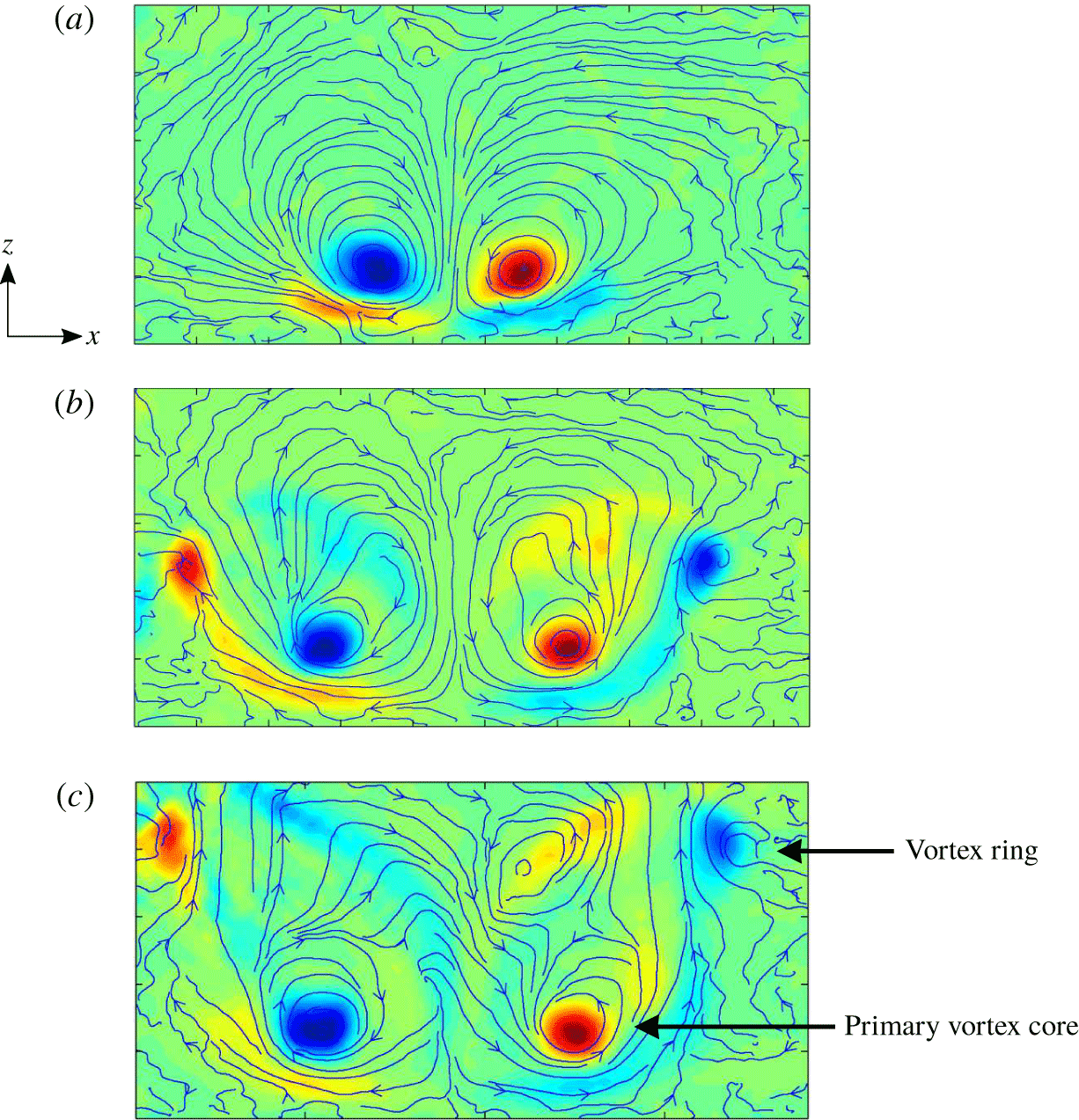
In order to confirm that the rising horizontal vortex structures observed over the valleys take the form of vortex rings, additional experiments were conducted to obtain transverse and longitudinal vorticity data. Transverse PIV measurements were predominantly taken through the valley. Figure 20(a–c) shows the development of the primary and secondary vorticity. The primary vortex core is visible in each frame: following wall interaction, it remains approximately in a single location.
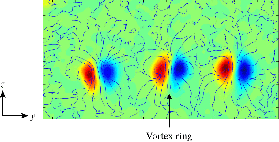
Figure 20(a) shows the initial generation of opposite-signed secondary vorticity in the valley. The secondary vortex structure rises vertically upward in each frame. In figure 20(c), we see the first evidence of a vortex ring over the valley. Red (counter-clockwise) and blue (clockwise) vorticity contours appear as a vortex pair over the valley, two sets per fundamental wavelength.
Particle image velocimetry measurements of the transverse cross-section through the valley, with streamlines and vorticity contours. Red indicates counter-clockwise rotation, and blue indicates clockwise rotation. The generation of secondary vorticity is seen, as is the formation of the vortex ring. Panels (a–c) are taken at  $t^{\ast }=4.6,7.5,$ and
 $10.4$, respectively. These structures correspond with the visualizations of figure 14.

Particle image velocimetry measurements of the longitudinal cross-section across three wavelengths with streamlines and vorticity contours taken at  $t^{\ast }=7.0$, showing the formation of three vortex rings. Red indicates counter-clockwise rotation, and blue indicates clockwise rotation. One of each pair of vortex rings is generated at each wavelength.

Particle image velocimetry measurements in the longitudinal plane are shown in figure 21. The longitudinal plane is perpendicular to the transverse plane, and is taken across three wavelengths of the hill. As such, we observe three distinct secondary vortex structures, each one forming over a valley. A key feature we observe in the streamlines superimposed onto the vorticity contours in figure 21 is the presence of upward velocity vectors between each of the vortex pairs. These upward velocity vectors indicate the approximate self-induced velocity of the secondary vortex structures, making them rise upward away from the ground.
It was expected that the three-dimensional changes observed in this study of a 2-D vortex pair interacting with a wavy wall would be remarkably similar to those observed in the complementary experiment of a vortex pair with the long-wavelength Crow instability interacting with a flat wall. However, the dynamics we observe via flow visualization and PIV are surprisingly quite different to those seen for either an unperturbed 2-D vortex pair impinging on a flat wall (e.g. Harris & Williamson (Reference Harris and Williamson2012)), or for a wavy vortex pair impinging on a flat wall (e.g. Asselin & Williamson (Reference Asselin and Williamson2017)).
Whilst the initial generation of secondary vorticity via vortex–ground interaction is fundamentally the same as has been observed in previous works, the topological differences following ground interaction quickly become apparent for the vortex pair impinging on a wavy wall. In this study, the secondary vortex loop and rising secondary vortex rings are the dominant three-dimensional flow feature. We do not observe any periodic secondary vortex instability such as was observed by Harris & Williamson (Reference Harris and Williamson2012). It is predicted that there is a critical spanwise wavelength (approaching a flat wall as you increase  $\unicode[STIX]{x1D706}$) at which the secondary vortex instability will again become the dominant, principal 3-D flow feature.
A surprising result arising from this work is that the mechanism by which the horizontal vortex rings are formed in this study greatly differ from the way in which they are formed for the ‘horizontal rings mode’ of a wavy vortex impinging on a flat wall. Asselin & Williamson (Reference Asselin and Williamson2017) observed that small-scale vortex rings are formed due to reconnection occurring between the primary vortex and the secondary vortex. Here, we do not observe this reconnection. Rather, the primary vortex remains intact, while the secondary vortex loop alone forms rising vortex rings, comprising two small-scale vortex rings per fundamental wavelength.
4 Discussion
Superposition of vorticity contour plots onto flow visualization. Red indicates counter-clockwise rotation, and blue indicates clockwise rotation.

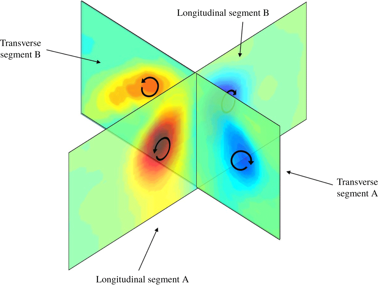
Transverse and longitudinal vorticity contours placed orthogonal to one another, revealing a vortex ring. The sense of rotation of each segment is shown. Red indicates counter-clockwise rotation, and blue indicates clockwise rotation.

In this section, we study thence three features of the flow. Firstly, we observe the formation of vortex rings from the secondary vortex loops generated in each valley. We also observe an increase in the rate of circulation decay of the primary vortex pair compared to a vortex pair impinging on a flat wall. The study of the decay of the primary vortex pair was a primary goal of this research, based on the idea that using a passive, ground-based obstacle may be an effective way to dissipate aeroplane trailing vortices near a runway. Lastly, a surprising result to arise from this study, is the lack of axial flow observed in the primary vortex pair upon interaction with the hillocks. At the onset of this research study, it was expected that we would observe significant axial flow in the primary vortex pair, in agreement with the complementary experiment of a wavy vortex pair interacting with a flat wall. In that experiment, Asselin & Williamson (Reference Asselin and Williamson2017) found that axial flow in the primary vortex cores was a primary factor in the three-dimensional topological changes they observed. However, we find that there is negligible axial flow in the primary vortex cores upon interaction with the wavy wall. Rather, we find that the three-dimensional flow we observe is a result of the formation of the complex secondary vortex structures shown in § 3.
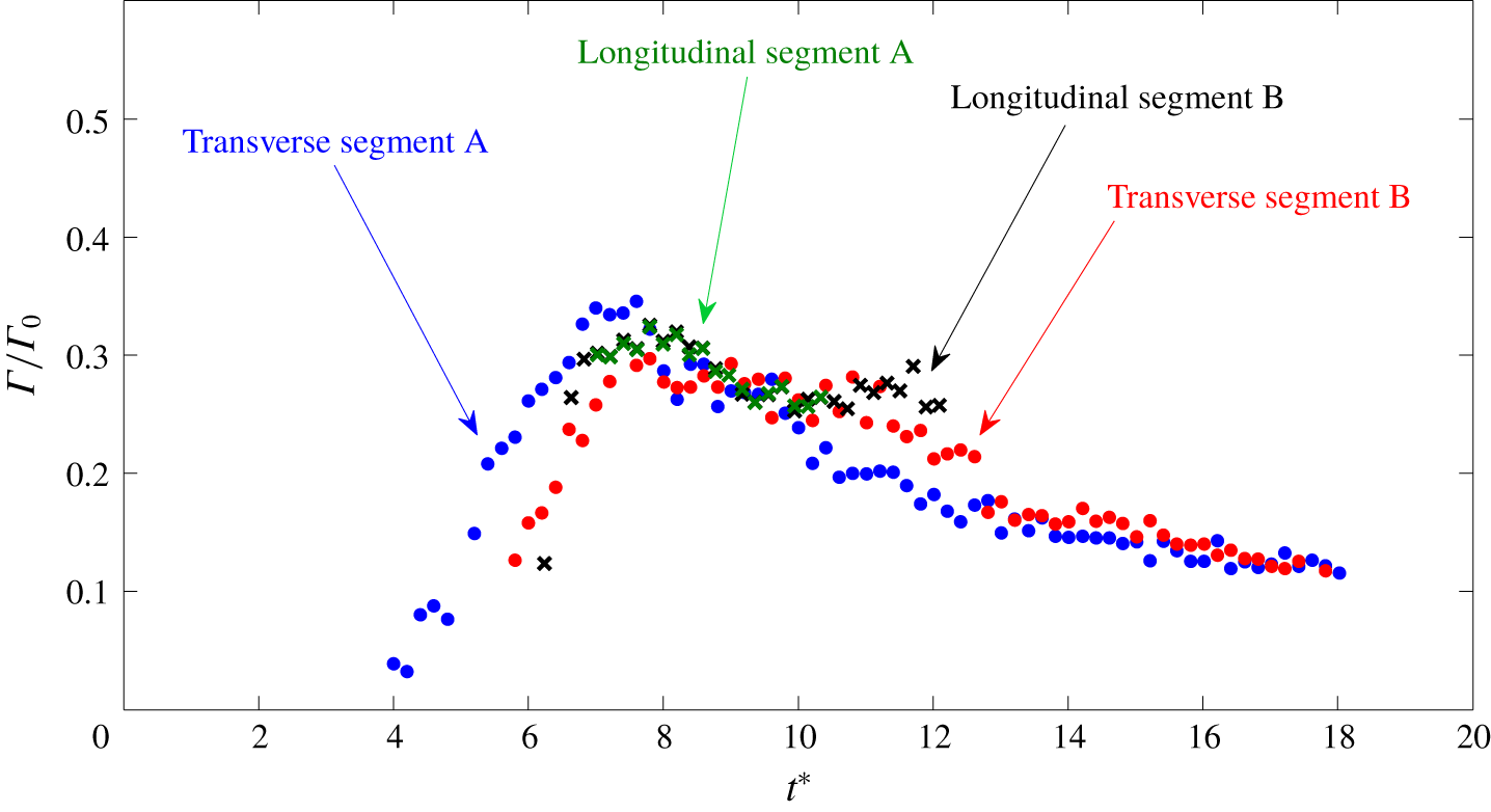
Circulation measured in four orthogonal segments of a vortex ring. The circulation across each segment of the vortex ring is approximately constant.

4.1 Further evidence showing the formation of a vortex ring from a vortex loop
The changing topology of a vortex loop forming a vortex ring is a fundamental process in phenomena such as hairpin vortices and the wake of rising and falling spheres. In turbulent shear flows, the local curvature of the legs of hairpin vortices produces an  $\unicode[STIX]{x1D6FA}$-shaped vortex loop, which draws the vortex legs towards each other and causes pinch off (Perry, Lim & Teh Reference Perry, Lim and Teh1981; Moin, Leonard & Kim Reference Moin, Leonard and Kim1985). Horowitz & Williamson (Reference Horowitz and Williamson2010) experimentally observed the pinch off process of a vortex loop behind a sphere into a vortex ring; flow visualization and PIV were used to confirm the presence of vortex rings.
In order to confirm the presence of rising horizontal vortex rings, we use circulation measurements from PIV vorticity contour plots in conjunction with our flow visualization. Figure 22 shows the superposition of vorticity contour plots onto full-flow visualization. It seems that our flow visualization exhibits a good representation of vorticity, particularly at early time stages. However, it is necessary to use vorticity measurements to confirm the presence of the rising vortex rings due to the difference in the rate of diffusion of fluorescein dye (with diffusivity  $\mathscr{C}$) and of vorticity. The Schmidt number
 $Sc=\unicode[STIX]{x1D708}/\mathscr{C}$ describes this relationship, and is approximately 1200 (Horowitz & Williamson Reference Horowitz and Williamson2010). Employing PIV, we place light sheets in both the transverse and longitudinal planes, orthogonally intersecting the region of one of the rising secondary vortex structures.
Figure 23 shows vorticity contours taken at the same height and non-dimensional time and placed orthogonal to one another in three-dimensional space. These four segments, labelled as longitudinal segment A and B, and transverse segment A and B, reveal a rising horizontal vortex ring.
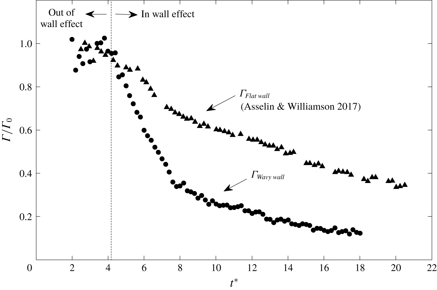
The circulation of each of the four segments shown in figure 24. As can be seen in figure 24, at  $t^{\ast }\approx 6.5$ the magnitude of the circulation of each segment in the orthogonal planes becomes roughly equal, with
 $\unicode[STIX]{x1D6E4}/\unicode[STIX]{x1D6E4}_{0}\approx 0.30$. From this point, the circulation around the entire secondary vortex structure is thus similar, confirming the formation of the vortex ring.
Circulation of the primary vortex core against time, for a straight vortex pair impinging on a flat wall (Asselin & Williamson Reference Asselin and Williamson2017), and a straight vortex pair impinging on a wavy wall.

4.2 Accelerated decay of the primary vortex
A primary goal of the interaction of vortex pairs with non-uniform walls is to trigger the rapid decay of the wake vortex by using a passive, ground-based approach. The introduction of a perturbed ground plane leads to accelerated circulation decay in comparison to a flat ground plane, as the flow quickly becomes three-dimensional, breaking up into smaller-scale structures.
Previous studies have considered the concept of using structural perturbations on the ground plane to increase the rate of circulation decay of a counter-rotating vortex pair (see Zheng & Wei (Reference Zheng and Wei2013), Kazarin & Golubev (Reference Kazarin and Golubev2017) and Stephan et al. (Reference Stephan, Holzäpfel and Misaka2013a,Reference Stephan, Holzäpfel, Misaka, Geisler and Konrathb)).
Figure 25 shows the development of circulation in our primary vortex pair following ground interaction. We show data from Asselin & Williamson (Reference Asselin and Williamson2017) as a comparison for a 2-D vortex pair impinging on a flat wall; this data is taken for a vortex pair with the same  $\unicode[STIX]{x1D6E4}_{0}$ and
 $b_{0}$, in the same facility at Cornell University. It is evident that the addition of the sinusoidal wavy wall accelerates the decay of the primary vortex pair. In the case of the 2-D vortex pair impinging on the wavy wall, the primary vortex core reaches 40 % of its initial circulation strength in
 $t^{\ast }=7.5$, whereas it takes
 $t^{\ast }>16.0$ for the wall with no perturbations and the same initial conditions to reach the same level of decay.
4.3 Absence of axial flow in primary vortex in comparison to Crow instability in ground effect
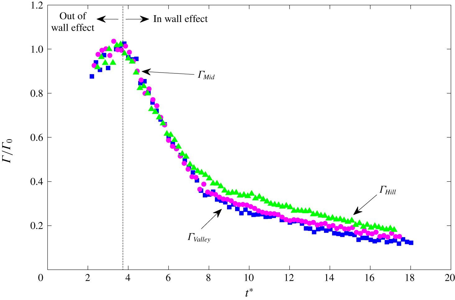
Circulation of the primary vortex core taken in the valley, over the hill, and midway in between. Each location of the primary vortex core decays at an approximately equal rate, which is consistent with a lack of axial flow within the primary vortex cores.

In the case of a vortex pair with Crow instability interacting with the ground, axial flow in the primary vortices was observed to be fundamental to the formation of 3-D vortex structures (Asselin & Williamson Reference Asselin and Williamson2017). For a vortex pair with Crow instability, the circulation is not constant along the length of the vortex tube. Namely, the ‘trough’ of the wavy vortex – the part of the vortex closes to the ground – has lower circulation values than at the ‘peak’ (see figure 5). Following interaction with the wall, the difference in circulation between the trough and peak regions is magnified. As a result of this difference, an axial pressure gradient is established between the troughs and peaks, leading to axial flow in the vortex tube. This axial flow is made evident by flow visualization, as the dye is seen to move from lower circulation regions (trough) to higher circulation regions (peaks) (Asselin & Williamson Reference Asselin and Williamson2017).
In contrast to Asselin & Williamson (Reference Asselin and Williamson2017), we observe very little axial flow in the primary vortex structures following interaction with the wavy wall. In the studied configuration, the dye remains relatively uniform along the length of the primary vortex (see for example figures 13 and 17). It is expected, however, that for a single perturbation at the wall, an axial flow would develop within the primary vortices.
Measurements of circulation around the primary vortex are shown in figure 26. The primary vortex circulation decays at an approximately similar rate for all three different spanwise locations. This is consistent with having only a small level of axial flow in the primary vortex.
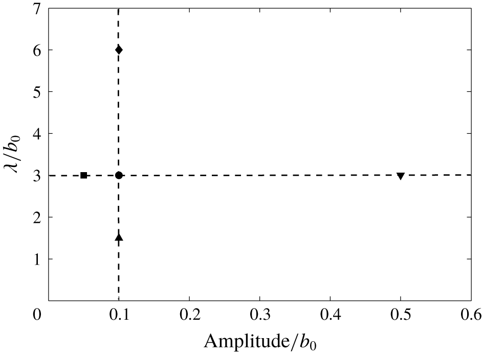
Plot showing the parameters of selected wavy walls. The wavelength  $\unicode[STIX]{x1D706}/b_{0}$, is plotted against the amplitude
 $A/b_{0}$. Symbols: ▪,
 $A=0.1~\text{cm}$,
 $\unicode[STIX]{x1D706}=6~\text{cm}$; ●,
 $A=0.2~\text{cm}$,
 $\unicode[STIX]{x1D706}=6~\text{cm}$; ▴,
 $A=1~\text{cm}$,
 $\unicode[STIX]{x1D706}=6~\text{cm}$; ▾,
 $A=0.2~\text{cm}$,
 $\unicode[STIX]{x1D706}=3~\text{cm}$; ♦,
 $A=0.2~\text{cm}$,
 $\unicode[STIX]{x1D706}=12~\text{cm}$.

5 Brief observation of vortex dynamics as a function of amplitude and wavelength of the wavy wall
Access to rapid prototyping facilities enabled us to investigate a set of different amplitudes and wavelengths of the periodic wavy ground plane. Several wavy wall configurations were explored, as indicated in figure 27. The amplitude of the wavy wall was varied while holding the wavelength constant, and the wavelength of the wavy wall was varied while holding the amplitude constant. As discussed in § 2, we used a wavy wall of amplitude of  $0.2~\text{cm}$ and wavelength of
 $6~\text{cm}$ throughout the current research, unless otherwise indicated.
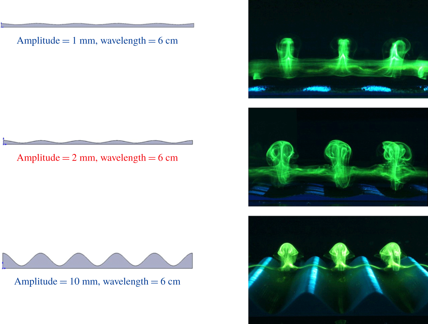
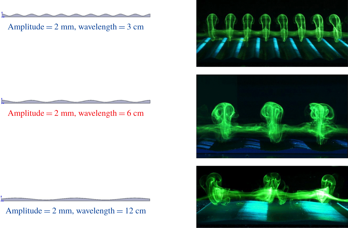
In figures 28 and 29, we present side view images of dye visualization for the variation of amplitude, and variation of wavelength. It is observed that the size of the secondary vortex structures scale with the ground-pattern dimensions. Across all studied parameters, the same phenomenon seems to be observed. We see secondary vortex structures moving up and away from the horizontal surface. In particular, the width of the secondary vortex loop is observed to scale with the wavelength of the hillock. If we were to look in plan view, we would see that the secondary vortex structures observed in figures 28 and 29 represent two vortex rings per fundamental wavelength.
Figure 28 shows the effect of changing the amplitude of the wavy wall while holding the wavelength constant. The formation of rising vortex rings is observed even at amplitudes as small as  $1~\text{mm}$, indicating that even very small structural perturbations at the wall can lead to distinct three-dimensional topological changes in the flow.
Figure 29 shows the effect of changing the wavelength of the wavy wall while holding the amplitude constant. Once again, we see the formation of the same secondary vortex structures across the given parameter range, even as the wavelength increases. In all cases, the primary vortex pair remains in its location following rebound, and two vortex rings are formed per fundamental wavelength. As the wavelength is increased, we observe that the secondary vortex structures are less coherent than at smaller wavelengths. This is unsurprising, as the case of an infinitely long wavelength would be a flat wall. The wavelength of the hillock dictates the width of the secondary vortex loop that forms; at a critical width it is expected that the secondary vortex loop will have insufficient self-induced velocity to rise upward, resulting in no formation of the vortex rings.
Side view flow visualization for changing the amplitude of the hillock, while holding the wavelength constant.

Side view flow visualization for changing the wavelength of the hillock, while holding the amplitude constant.

6 Practical applications
As discussed earlier, this research can be extended to practical applications. The focus has been to mitigate the wake vortex hazard by reducing the circulation of trailing vortices above a runway. In the present work, an understanding of the complex three-dimensional dynamics that arise upon the interaction of trailing vortices with perturbed walls is critical to this technique. We have shown that the addition of sinusoidal perturbations to the ground is an effective mechanism to accelerate the decay of circulation of vortex pairs. These perturbations generate coherent secondary vortex structures over a range of amplitude and wavelength parameters, as shown in figures 28 and 29.
A way of exploiting these fundamental dynamics is to install obstacles at the ground in the vicinity of airport runways, to accelerate the decay of the primary vortex pair. As aforementioned, these ideas have been explored by the research group at DLR, for example Holzäpfel et al. (Reference Holzäpfel, Stephan, Misaka and Körner2014), Stephan, Schrall & Holzäpfel (Reference Stephan, Schrall and Holzäpfel2017) and Wang et al. (Reference Wang, Zhao, Schlüter, Holzäpfel and Stephan2017). Using large eddy simulation and realistic large aircraft parameters, Stephan et al. (Reference Stephan, Holzäpfel and Misaka2013a) show that the typical separation time of a medium aircraft following a large aircraft can be reduced by as much as 50 % upon introduction of an obstacle at the ground. A series of plates, rather than a single obstacle, takes into account realistic navigational and safety costs at airports. This concept was taken into real-flight experiments using a series of six vertical hinged wooden plates of size  $4~\text{m}\times 2.2~\text{m}$ (
 ${\approx}0.1b_{0}\times 0.2b_{0}$). These plates were placed
 $10~\text{m}$ apart in a line perpendicular to the path of a vortex pair generated by a modified Gulfstream G550 aircraft at Oberpfaffenhofen airport (Holzäpfel et al. Reference Holzäpfel, Stephan, Misaka and Körner2014). Flow visualization and lidar measurements confirmed the efficacy of these ground-based obstacles, as a significant reduction in the circulation of the trailing vortex pair was observed.
In the present study, we have shown that even small amplitude perturbations at the ground plane ( $A\approx 0.1b_{0}$) can produce sufficiently strong secondary vortex structures to significantly reduce the circulation of the primary vortex pair. For aircraft landing at airports, a typical descent angle with the ground is
 $3^{\circ }$. At these angles, we can assume that the length of the vortex coming into contact with the obstacle(s) is approximately horizontal. As such, we would expect the same phenomenon (accelerated decay of circulation) to occur. It is apparent that the introduction of obstacles at the ground to trigger the formation of three-dimensional secondary vortex structures is a conceivable means to accelerate the decay of trailing vortices.
7 Conclusions
In this study, we examine the dynamics of a two-dimensional (straight) vortex pair as it impinges upon a wavy wall. In a practical sense, we are motivated to understand the breakup and decay of trailing vortices formed in the wake of an aircraft. This is in order to diminish the vortex wake hazard of one aircraft on a following aircraft, in the aircraft’s approach to or departure from a runway.
The flow studied here is the complement to the case where an unstable wavy vortex pair impinges upon a flat ground plane. The formation of three-dimensional vortical structures turns out to develop quite distinctly between the two studies. In one case, we have a counter-rotating vortex pair descending vertically and developing the wavy ‘Crow’ instability (Crow Reference Crow1970) which then impinges on a plane, and involves distinct axial flows within the primary vortices. In our present case, we have straight vortices impinging on a wavy wall or ground plane, but surprisingly the axial flow phenomenon is not a fundamental characteristic of the vortex dynamics in this case. However, in both flows the resultant principal vortex dynamics involves the formation of mini vortex rings.
In the present case, the rising vortex rings consist solely of secondary vorticity induced by the interaction of the straight vortex pair with the wavy wall. This is due to the nature of how the secondary vortex structures are created. It is found that the descending vortex pair first interacts with the hills of the ground plane before the valleys, causing earlier generation of secondary vorticity over the hills. By the time secondary vorticity is generated in the valleys, the secondary vorticity generated over the hills will have almost advected over the top of the primary vortex (see for example figures 12, 13 and 19). This results in the formation of secondary vortex loops in the valleys, two per fundamental wavelength. The self-induction of these loops on themselves causes them to rise upward away from the primary vortices. These loops pinch off into rising vortex rings. For the wavy wall configuration studied, it is found that the primary vortex will reach  $40\,\%$ of its initial circulation strength in less than half the time required for a vortex pair impinging on a flat wall. The breakup of the vortex pair is ably achieved by the 3-D vortex interactions of the present study.
The pinch off of vortex loops into vortex rings is also observed in several other flows, such as hairpin vortices in turbulent boundary layers (Cantwell Reference Cantwell1981; Robinson Reference Robinson1991; Panton Reference Panton2001) and the vortex rings formed behind rising and falling spheres (Horowitz & Williamson Reference Horowitz and Williamson2010).
A surprising result of this research was the lack of axial flow in the primary vortex pair in the studied hill–valley configuration. Approaching this study as the complementary experiment to the work of Asselin & Williamson (Reference Asselin and Williamson2017), it was expected that we would see significant axial flow as the driving mechanism behind the formation of vortical structures. Asselin & Williamson (Reference Asselin and Williamson2017) observed this axial flow as the movement of dye along the primary vortex core. In the present study, however, we do not observe any clear axial movement of dye within the primary vortices. Furthermore, we observe a negligible difference in the circulation of the primary vortex pair along the length of the vortices, indicating that there is no pressure gradient established in the primary vortex cores. Rather, it is the formation of coherent secondary vortex structures that leads to the formation of small-scale vortex structures.
The accelerated decay of trailing vortices upon interaction with a perturbed wall is one practical application of these experiments. Employing blunt objects on the ground helps to break up impinging vortex pairs, as one might expect. Rather than exploiting natural instabilities out of ground effect, passive ground-based systems aim to accelerate the decay of the trailing vortices near the ground, where the wake vortices pose the most danger to following aircraft. The generation of coherent vortical structures following interaction with a non-uniform wall is also observed by the research group at the German Aerospace Center (see for example Holzäpfel et al. (Reference Holzäpfel, Stephan, Misaka and Körner2014), Stephan et al. (Reference Stephan, Holzäpfel and Misaka2013a,Reference Stephan, Holzäpfel, Misaka, Geisler and Konrathb, Reference Stephan, Schrall and Holzäpfel2017), Wang et al. (Reference Wang, Zhao, Schlüter, Holzäpfel and Stephan2017)), wherein the impingement of a vortex pair onto obstacles yields a significant reduction in circulation in the primary vortex pair. The introduction of perturbed-ground planes and the resultant generation of secondary vortex structures is an effective passive, ground-based method of accelerating vortex decay. Whichever passive structure is selected, it is obviously essential to have it compliant such that it does not damage aircraft.
Acknowledgements
The authors would like to thank Nathan Bristow (PhD candidate, University of Notre Dame) and Professor Robert Shepherd (Organic Robotics Laboratory, Cornell University) for their assistance in the construction of the transparent wavy wall. The authors would also like to thank the American Australian Association Education Fund and Zonta International Amelia Earhart Fellowship for their support.
Declaration of interests
The authors report no conflict of interest.
Appendix A. Using flow visualization to construct 3-D images
Parametric solution schematic generated in SolidWorks of the generation of secondary vorticity. Side view and plan view flow visualization images taken at  $t^{\ast }=5.2$ were used to map the feature (see figure 12c,d).

In addition to schematics, we also constructed a SolidWorks schematics of the flow using our flow visualization data. Using side view and plan view images that had been taken simultaneously, we used secondary flow visualization to map the location of secondary vorticity.
Using the  $x{-}z$ and
 $x{-}y$ planes (figures 12c and 12d, respectively), we match the
 $x$-,
 $y$- and
 $z$- coordinates of the secondary vortex in Matlab. In doing so, we are able to render an accurate 3-D representation of the secondary vortex. A parametric solution consisting of
 $z(x)$ and
 $y(x)$ solutions describes the three-dimensional shape.
The  $x{-}z$ plane is represented by a second-order Fourier series, in the form
 $$\begin{eqnarray}z(x)=a_{0}+a_{1}\cos (xw)+b_{1}\sin (xw)+a_{2}\cos (2xw)+b_{2}\sin (2xw).\end{eqnarray}$$
The  $x{-}y$ plane is represented by a sine curve, in the form
 $$\begin{eqnarray}y(x)=A\sin (Bx-C)+D.\end{eqnarray}$$
Using these two equations, we generate a parametric solution describing the secondary vorticity and visualize it via SolidWorks in figure 30.