1. Introduction
The early work on probabilistic causality, especially that of Salmon (Reference Salmon1980) and Suppes (Reference Suppes1970), made clear that we need to discriminate among purported causal factors, all of which have a probabilistic impact on an effect, ruling out those which are screened off by common ancestors. Subsequently, it also became clear that such a degree of discrimination was insufficient, that the context in which probabilistic impacts are found must be more acutely observed. The Contextual Unanimity Thesis (CUT) emerged as the leading proposal for sifting out those factors which promote (or prevent) some effect. CUT is the idea that causes are context-independent. It claims that C causes E only if C raises the probability of E across all homogeneous reference classes created by a partition using all other factors causally relevant for E. Footnote 1 This thesis has been endorsed by many of those attempting to make sense of the concept of probabilistic causality—among others, by Cartwright (Reference Cartwright1979), Skyrms (Reference Skyrms1980), Eells and Sober (Reference Eells and Sober1983), Humphreys (Reference Humphreys1989) and (in a weakened form) Cartwright again (Reference Cartwright1989). According to this requirement, we should not say that imbibing a poison causes death if, in fact, there is a perfect antidote, for in the reference class of those treated with the antidote the poison is in efficacious, which result defeats the causal claim. This may seem like an odd requirement to impose upon causal talk, for there seems nearly always to be available some reference class in which a putative cause will fail to raise the probability of its effect: namely, the reference class in which the object, thing, or space-time slice of interest is going to be immediately obliterated, before the causal mechanism can operate to completion. Thus, we should say that firing squads fail to cause the deaths of their victims, since an imminent heart attack could preempt that eventuality.Footnote 2
A plausible response, and defense of CUT, could invoke conversational implicature, ruling out pre-emptive or other annoying causal factors which are clearly, by conversational context, meant to be ruled out. But such maneuvering aims to save unanimity theory in order to account for ordinary language. Probabilistic causality is not primarily an ordinary language investigation, as the long history in ordinary discourse of assuming that causes are sufficient for their effects surely demonstrates. CUT is, at best, a poor aid in understanding ordinary language causal talk, whereas the concept of objective homogeneity does the real work in helping us make sense of probabilistic causality, if only in combination with a known causal structure.Footnote 3
First we need to clarify some of the terms of the discussion, before turning to a critique of CUT. Our interest is the conditions for C being a probabilistic cause of E. The relevant concept of probability is that of physical probability or objective chance, presumably under a propensity interpretation (or, perhaps, frequencies in an infinite hypothetical sequence of trials—the exact story is not the issue here). We are not directly concerned with token causality—the conditions for a token event to be a token cause of another token event—but with type causality, such as whether smoking causes lung cancer.Footnote 4
We discuss, and distinguish, two concepts that some may have confused: contextual unanimity and objective homogeneity. Both appeal to populations of events and their partitions. The cells in a partition are types of events, in particular, events which share some fixed setof values.Footnote 5 Both contextual unanimity and objective homogeneity begin with a partition where each cell (alternatively: subpopulation, reference class, or context) is homogeneous for the effect. A cell H i is homogeneous for an effect E if there is no computable-beforehand property A which makes a difference to the probability of E for events in the cell.Footnote 6
There are two basic concepts of homogeneity, namely:
Objective Homogeneity: A population (or subpopulation) H i is objectively homogeneous for an effect E if there is no computable-beforehand property A which makes a difference to the probability of E. That is, for any such A within
 $H_{i}$
,
$P(E\mid A) =P(E\mid \overline{A}) $
.


Epistemic Homogeneity: A population (or subpopulation) is epistemically homogeneous for an effect E if we do not know, of any computable-beforehand property A, that it makes a difference to the probability of E.
When we are acting as practical investigators of causality, we are constrained by the limits of our knowledge, so epistemic homogeneity has a role to play in accounting for scientific method and pragmatic judgment. But, on our view, objective homogeneity is the regulative concept required for analyzing the goal of our methodological efforts, namely causal structure.
Employing causal Bayesian networks (treated in more detail subsequently), we can, in fact, introduce a third kind of homogeneity that explicitly reflects this regulative role of objective homogeneity:
Model Homogeneity: Given a causal model M, a population (or subpopulation) identified by a set of observed variables O in M is homogeneous for an effect E if there is no other variable in M which is a non-descendent of E and the observation of which makes a difference to the probability of E.
If our understanding of the causal structure of the world can be represented in a causal model, then our current best understanding of homogeneous contexts or subpopulations is given by its model homogeneities. As we learn more about the world we develop and refine our best models, and our epistemically homogeneous reference classes get refined in turn. We may reasonably hope that a sequence of such refinements is aimed at the truth, which is the set of model homogeneities for the true causal model. In the meantime, prior to Keynes's limit, we work with models that are false and our epistemic homogeneities may well mislead us. Such is the fate of every inductive agent.
Note that, just as in Wesley Salmon's early work on statistical relevance (Salmon Reference Salmon1974), homogeneity (of every kind) is concerned with quantities: it is essential for homogeneity to obtain that the probabilities do not deviate. One of the attractions of CUT is that it has far laxer standards—simply that differences in probability across contexts all pull in the same direction, at whatever magnitude. We shall argue that the attractiveness of laxity is strictly superficial.
2. Unanimity and Homogeneity
Contextual unanimity is properly defined in terms of objective homogeneity (cf. Eells Reference Eells1985):
Contextual Unanimity: A population is contextually unanimous for C with respect to E if and only if in all cells (contexts) H i in an objectively homogeneous partition,Footnote 7
$P(E\mid C) > P(E\mid \overline{C}) $
.

The corresponding thesis is the claim that causes are properly identified in terms of unanimity. More formally,
Contextual Unanimity Thesis (CUT): C causes E only if the background population is unanimous for C with respect to E.
Whereas unanimity theory supposes that what is causally efficacious (e.g., worthy of the rubric “causal power,” in Cartwright's language) must be so across contexts, homogeneity theory adopts the exactly opposite position: that causal factors are context-dependent and, to get the causal story right, we must relativize causal claims to a specific context. Not only need the causal powers push in the same general direction, but they need to push with the very same strength. Anything less does in fact average disparate powers, which is not good enough even for government work.Footnote 8 Hence, our initial thesis is:
Objective Homogeneity Thesis (OHT): C is causally relevant to E in the homogeneous context
$H_{i}$
only if, within
$H_{i},$
$P(E\mid C) \neq P(E\mid \overline{C}) $
.


Objective homogeneity was first championed by Salmon (Reference Salmon and Colodny1970) as a key to statistical explanation. It takes seriously the relativization of causal claims to populations, advocated by Eells (Reference Eells, Skyrms and Harper1988), perhaps more seriously than Eells did himself. The requirement of OHT is that causal claims be relativized to objectively homogeneous reference classes (the cells H i), so that the introduction of any further putative causal factor cannot change the probability of the effect to any degree whatsoever. If causal claims are not so relativized, they can be arbitrarily wrong about the causal strength (effect size).
Note that whereas CUT is specifically about a state C promoting the outcome state E, OHT is about whether variable C is causally relevant to variable E. But whenever one state of a variable is promoted, another must be demoted, so when speaking of variables causing one another, causality just is causal relevance. It is also worth noting that one can always recover the CUT verdict from the OHT conditions, but not the other way around.
There is a clear and direct relation between the properties of contextual unanimity and objective homogeneity. Unanimity is defined in terms of homogeneity, so there is a sense in which any case having the property of being objectively homogeneous must trivially also have the property of being contextually unanimous. That is, if we restrict our context to the single cell satifying our objective homogeneity requirement, that context will be unanimous for the effect. Of course, the aim of CUT is to find a useful criterion that generalizes beyond such narrow contexts, so the theses are distinct; OHT is quite significantly stricter than CUT.
It is worth noting that a weaker version of the homogeneity thesis can be had by substituting epistemic for objective homogeneity—that is, relying upon the model homogeneities of our currently best model. This would produce a criterion far easier to meet: it would require only that we not know of any causal factor which could partition the reference class to produce distinct probabilities of the effect. And it is surely true that as a practical matter we are often satisfied with epistemic homogeneity. Indeed, Dupré and Cartwright appear to believe that epistemic homogeneity is all that we can ever have:
But we have been arguing that however finely we partition the population, we cannot know from the statistics that we have anything better than an average causal upshot. (Dupré and Cartwright Reference Dupré and Cartwright1988, 530)
Science progresses, quite explicitly in the form of experimental methods, from crude epistemically homogeneous classes to identifying inhomogeneities to more refined models and so improved epistemically homogeneous classes (as we pointed out in Korb Reference Korb and Sankey1999). And in some cases science progresses to what is arguably objectively homogeneous (cf. Bell's theorem). Thus, objective homogeneity provides the metaphysical norm toward which epistemic homogeneity can tend. Dupré loudly denounces such a view as hiding behind a “metaphysical fig leaf” (Reference Dupré1993). But a denunciation is no counter argument. If the history of science makes anything clear, it is clear that a scientific explanation which omits unknown causal factors may be wrong, discovered to be wrong, and properly be replaced by an account which incorporates those variables. Dupré's dismissal of metaphysics would simply leave these known facts about science mysterious.
Objective homogeneity in OHT provides the stricter standard that can make sense of our normative aspirations.
3. Problems with CUT
CUT fails to provide an adequate criterion for probabilistic causality simply because it is not strict enough. If we partition only as finely as required to satisfy contextual unanimity, we have effectively declared that causation has only direction but not strength. CUT is equivalent to creating a homogeneous partition and then agglomerating disparate capacities to bring about an effect, on the grounds that they operate in the same direction, regardless of their strengths. As Dan Hausman emphasizes,Footnote 9 the appeal of CUT is that it appears to make causal talk useful. Instead of requiring us to identify, even if only in principle, all the factors needed for objective homogeneity, we can take the more relaxed approach of identifying only such factors as are needed to force a common causal bearing (direction of impact) on the effect. The difficulty with this line of thought is two-fold. First, in non-microphysical cases we are no closer practically to locating those factors needed for a common causal bearing than we are to locating those needed for objective homogeneity itself. If we can happily assert that smoking causes cancer, for example, it is not because we know that there are no countervailing forces where smoking is neutral or even preventative for cancer. So CUT fails even as an account of ordinary causal talk. But second, this line of thought—aiming to account for the utility of and/or the pragmatics of ordinary causal language—is a diversion from giving a normative, metaphysical account of causation, and not the very same thing. If we can connect the distinct metaphysics and epistemics of causation, we will have achieved our goal.
Beyond the considerations about how causal talk works, CUT seems to have little going for it. If some treatment raises the probability of survival in one category of cancer patient by 300% and and in another by 5%, this is not a trivial difference to be papered over by talk of “causal power.” Effect size matters! Indeed, the multivariate methods of statistics used to analyze contingency tables and make sense out of such cases unsurprisingly depend explicitly on exact estimates of just such differences. A methodology for causal inference founded upon a metaphysics which ignores them would simply be a non-starter.
3.1. Varieties of Populations
Taking particular values of C and E, there are four kinds of population to consider (where C abbreviates
 $C=c$
for some c, etc.):
1. Positive case: C raises the probability of E in all objectively homogeneous cells. In this case we can say C promotes E, or sometimes just C causes E.
2. Negative case: C lowers the probability of E in all objectively homogeneous cells. In this case we can say C prevents E, and it is strictly parallel to the positive case.
3. Mixed case: C raises the probability of E in some cells and lowers the probability of E in others. Most real cases appear to be like this.
4. Neutral case: C is always irrelevant for E.
The neutral case has generally been taken to be non-problematic, with the conclusion that C is not a cause of E. Later, we see where this can fail.
In the mixed case, an uncompromising CUT advocate would insist that C is simply not a cause of E, regardless of it having measurable effects.Footnote 10 Eells' insistence on relativizing to contextually unanimous subpopulations in fact puts him partway between that extremism and OHT. Eells' view absorbs all mixed cases into one of the other three cases, by relativizing the causal claim to some, but not all, the factors which identify an objectively homogeneous reference class. Under either interpretation, CUT is mixing together distinct cells in the homogeneous partition. Dupré and Cartwright correctly complain that, despite the unanimity requirement, all that we really have are “causal upshots”—an average of a variety of causal powers (even though they happen to point in the same direction).
As we just mentioned, this is a problem if we should like to make sense of multivariate methods of causal discovery, which crucially depend upon effect sizes (see, e.g., Korb and Nicholson Reference Korb and Nicholson2003; Spirtes et al. Reference Spirtes, Glymour and Scheines2000). It is also a problem when we attempt to make sense of causal interactions.
3.2. Mixtures and Interactions
In the linear case one cause interacts with another when the effect is not simply the sum of independently operating causal forces. Contextual unanimity does not have the tools to make sense of these causal interactions. A strict CUT theorist must claim that causes cannot interact, because according to CUT, neither positive nor negative causes can be interacting, and mixed causes are not causes at all. But we all know that causes do interact, so Eells and others have concluded that interaction happens precisely in the mixed case: where the valence of a cause reverses from positive to negative across contexts.
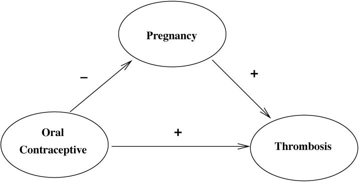
Yet mixed cases are neither necessary nor sufficient for causal interaction. They are not necessary because causes may interact by reinforcing each other beyond their individual effects (synergy or potentiation), by preempting one another, as well as by cancelling each other out in an exclusive-or relation (as, for example, alkali and acid can do). They are not sufficient because you can get a valence-reversal without interaction, via dual (multiple) causal pathways: for example, oral contraceptives do not interact with pregnancy to provide a mixed case for thrombosis—there is merely a multiple-path dependency (see Figure 1).
Multiple paths to thrombosis.

4. Problems with OHT
We shall now consider some objections to OHT. Glennan has recently objected that homogeneity forces us only to treat fully specified complexes of causal factors, which are unnatural and unwieldy; Dupré and Cartwright contend that homogeneity does not work in any case, since it fails for dual capacity scenarios. Neither objection can be sustained—although the possibility of dual capacities (in the form of precisely counteracting multiple pathways) will in the end force us to elaborate OHT with explicit reference to causal structure.
4.1. Glennan's Objection
In his discussion of contextual unanimity in the units of selection debate in evolutionary theory, Glennan argues:
if one requires context independence [i.e., contextual unanimity] for an entity to be a unit of selection, the unit of selection will inevitably be the entire genome. (Reference Glennan2002, 122)
This for the reason that there is very widespread interaction across loci, with alleles at some potentially negating or reversing the developmental effects at others, and all in such a complex interrelation that we cannot seriously expect the causal impact on reproduction to be unanimous without accounting for the entire nexus. So we will not get unanimity until we conjoin a great many background conditions into the cause. Glennan considers this an unwelcome result since it appears to trivialize the debate on units of selection.
But perhaps that debate should be trivialized. The same criticism must apply to OHT, as it is the more demanding requirement. If fixing the entire genomic background is required to achieve contextual unanimity, it will certainly also be required to find homogeneous reference classes for selection. To be sure, OHT here has a purely linguistic advantage over CUT: it asserts causality of the single gene (so long as there is any H i where it makes a difference), whereas CUT must assert causality only of the conjunction of all factors required to achieve unanimity.
The same point can be put in a simpler domain than the units of selection debate. Glennan also says,
Now it is possible to accept this consequence of contextual unanimity—to say that generalizations like the one that smoking causes cancer are false. (Reference Glennan2002, 124)
Presumably, if we homogenists are constrained to deny such an evident truth as that smoking causes cancer, then we are in trouble. But we are not. Taken as a general claim, homogenists can readily affirm the efficacy of smoking because there is at least one context in which it has the requisite probabilistic impact. Taken as a specific claim, we can say it is ambiguous and ask for a context. Within a context its truth or falsity will be clear. In support of the homogenist's treatment of the general claim, some plausible account, under implicature, can be made ruling out known or easily anticipated cases where the causal power of smoking is negated or reversed. The same defense applies to Eells, though not to strict unanimists (if there are any). But this line of consideration is irrelevant to the metaphysics of causation.
Returning to the genome, it is entirely likely that a less trivializing account of the units of selection debate can be made out of pragmatic considerations. In any case, as with smoking, we can certainly say that particular alleles cause particular characteristics, although no doubt only and always in particular circumstances which may never be fully accounted for. Objective homogeneity provides a regulative, normative account of causality and not necessarily a pragmatic account accessible in the short term. But rather than dismissing this verdict as a metaphysical pipe dream, why shouldn't we believe that a Bayesian network that fully depicts the causal structure of, say, human ontogeny would require variables representing every locus in the human genome? It would surely require that—and more, since humans do not develop in a vacuum.
4.2. Dupré and Cartwright's Objection
Dupré and Cartwright (Reference Dupré and Cartwright1988, section 4) argue that Eells' relativization of causal claims to populations (and, by extension, ours to homogeneous reference classes) fails in the case of dual capacities. We can use Hesslow's famous example (Hesslow Reference Hesslow1976) (Figure 1): oral contraceptives increase the risk of thrombosis in women who would not otherwise have become pregnant, but decrease that risk in women who would otherwise have become pregnant.Footnote 11
Of this example, Dupré and Cartwright say:
[This] criterion [unanimity and/or homogeneity]…yields the conclusion that in this population contraceptives do not prevent thrombosis (via prevention of pregnancy). The reason, we may all agree, is trivial. We have held pregnancy fixed…(Reference Dupré and Cartwright1988, 529)
If we hold pregnancy fixed, then contraceptives can only reinforce the tendency that pregnancy has (in one subpopulation) to produce thrombosis (and with similar result in the other subpopulation). But this is obviously wrong, as Dupré and Cartwright immediately observe:
[Many] women will in fact have been saved from thrombosis by the pills; without the pills they would probably have become pregnant and run a high risk of thrombosis.
Well, of course! If you hold fixed those who actually do become pregnant, etc., then you will run a very high risk of confusion in interpreting your experimental results. That is, in fact, the whole point behind Cartwright's refinement of her causality condition, CC*, elaborated in her Nature's Capacities and their Measurement (1989). A homogeneous reference class traditionally does not refer to intermediate effects (or any effects in the future of C), though it does require reference to the subjunctively identified subpopulations (captured retrospectively by CC*), such as those women who otherwise would have become pregnant—as we have discussed at length elsewhere (Korb Reference Korb and Sankey1999).
By confusing the subjunctive and indicative moods, Dupré and Cartwright have wrongly concluded that relativizing causal claims to homogeneous classes continues to mix causal capacities. Nevertheless, there are cases of dual capacities where OHT fails.
4.3. Causal Neutrality in Simple Worlds
When we identify homogeneous reference classes we are considering holding fixed all causally relevant factors prior to the one in question. Pregnancy comes after the factor in question (the pill). Of course, the subjunctive property comes before, which is what we were relying upon. We do not know precisely how to analyze such subjunctive properties, but presumably it is to be done in reference to a richer causal nexus than that described in Figure 1, with multiple hidden causes prior to taking the pill fixing an objective probability of falling pregnant without the pill. But what if the world is simple? What if there really are only three variables that describe the world?
If the world is as simple as Figure 1, and if the parameters exactly balance, so that the pill has no net probabilistic impact on thrombosis, then OHT advises that there is no causal relation between them. But that is wrong—we are assuming that Figure 1 is the right causal model, after all! So, it turns out that in the end, objective homogeneity alone cannot do the work we require of it.Footnote 12
We might be tempted simply to extend the partitioning conditions of OHT to incorporate downstream events, since, after all, observing Pregnancy in the neutral Hesslow case reveals the causal connection between the pill and thrombosis. Furthermore, allowing downstream variables need not resurrect the Dupré–Cartwright objection about falsely concluding that contraceptives only promote thrombosis, because it is a principle of homogeneity theory to require specification of the context, explicitly or implicitly. It is no error to say that, given that we know someone is pregnant, the pill does not prevent pregnancy; nor in that case can it be neutral for thrombosis.
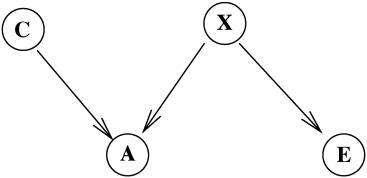
Nevertheless, this future-fixing OHT is inadequate for another reason: it sanctions the ascription of causality to non-causes. Consider the network of Figure 2. If we are allowed to observe the effect A, then we induce a probabilistic dependency between C and E (because the path from C to X becomes active, as explained in Section 5.1). But there is no sense in which C causes E here, even if it is known in advance that its effect A will hold.
Failure of future-fixing.

4.4. Intransitivity
On reflection OHT has an obvious problem: it ignores causal structure. Being exclusively probabilistic (and temporal), it cannot but mishandle exact balances. But if we move beyond probabilities to appeal to causal structure itself, we may wonder why we should bother with the probabilities at all. Indeed, a plausible conjecture for a satisfactory criterion of causality is the transitive closure over directed causal links in a causal graph. In that case, we could deploy our best causal discovery programs, for example, and simply examine the resultant graph to see whether X and Y are connected by a directed chain. Unfortunately, transitivity over direct causal links does not hold (Cooper Reference Cooper, Glymour and Cooper1999; Hitchcock Reference Hitchcock2001b; Pearl Reference Pearl2000). There are strange cases where, although X causes Y and Y causes Z, it just is not the case that X causes Z. For example, suppose Y describes how a terrorist pushes a detonator (with his left hand or his right hand) and Z an explosion. Then if X indicates whether a dog bites the terrorist's right hand, it may well have an impact on Y: if the dog bites the right hand, the terrorist will push with the left and otherwise with the right. But in either case the bomb will explode, so the dog's bite has no impact whatsoever on that outcome. We need a criterion of causality where X does not here cause Z. Footnote 13 It is only in cooperation that causal structure and probabilistic impact can identify general causal structure.
5. Wiggle Logic
On OHT, the most natural kind of causation is similar to what Eells calls “causal relevance.” We approach the problem by considering what happens probabilistically when we intervene upon (wiggle) the causal variable C in an attempt to fix its value to some c, which we represent I C=c (or simply I C).Footnote 14
In the spirit of OHT we could say that one variable C causes another E in a causal Bayesian network precisely when there is some causal context and some possible manipulation of C which is followed by a change in the distribution on E. In particular, a direct link should guarantee causation, given a causal Bayesian network which is also a perfect map.Footnote 15 A natural way to interpret causal relevance is via manipulations of C given observations of other variables O:
Causal Relevance (CR): C causes E with respect to G/O if and only if

Here, G/O means we have a causal graph G in which the variables O have been observed. O therefore identifies the background in which the causality question is raised, and O ' the context in which it is answered.Footnote 16
5.1. Intervention and Activation
We have begun talking about intervening on variables rather than just observing (or conditioning on) them. Most of the literature on probabilistic causality has used notions of intervention, especially in reference to experimental procedure, but without clarifying the relation between intervention and observation. Recent work in Bayesian networks has developed tools to represent both formally.
Technically, the best way to represent
 $I_{C=c}$
in a Bayesian network is to add a parent node
 $I_{C}$
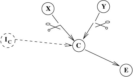
to C, allowing for any kind of success rate in manipulating the value of C (Korb and Nicholson Reference Korb and Nicholson2003). It is best in the sense that it is the most flexible, for it can represent imperfect, as well as perfect, control—that is, it can represent manipulations that may fail to fix the value of C, as well as those which are guaranteed to succeed regardless of the state of the parents of C. Adding the intervention variable I C also allows us to represent any kind of interaction between the manipulation and any alternative causes.Footnote 17 Regardless, in the case usually imagined (if unusually realized), I C indeed exerts perfect control over C. In that case, it is easiest to represent the intervention by cutting all arcs into C, and then fixing
 $C=c$
.Footnote 18
Under perfect control, the two representations are equivalent, although only the arc-cutting representation will be a perfect map. However, since they are equivalent, it follows that observations of I C (i.e., manipulations of C) cannot induce a probabilistic dependency with anything causally upstream from C. Footnote 19 In particular, C and E cannot then have any common cause inducing a probabilistic dependency between them. Nothing in the discussion will hang on the difference between perfect and imperfect control, so we shall assume perfect control, while continuing to refer to I C as the potential controlling variable.
Interventions and observations will have no probabilistic impact upon downstream events if they are blocked (d-separated) in the context O. Footnote 20
Blocking:
$\Phi \,\in \mathrm{Paths}\,(C,E) ,$
is blocked in G/O if and only if O d-separates C from E in G,

where Paths(C, E) is the set of all directed paths from C to E. Equivalently, Φ is blocked if and only if
 $\exists Z\left(Z\in \Phi \wedge Z\in O\right)$
.Footnote 21
What is doing the blocking (or not) in these cases is a set of observed variables O. What we specifically need for our Wiggle Logic is the concept of paths being “blocked” or not either because of such observations or because a direct connection between two variables
 $X\rightarrow Y\in \,\mathrm{Paths}\,(C,E) $
has been otherwise blocked—for example, by hypothetically introducing a previously unknown variable between X and Y and observing its value. Let R stand for a set of restrictions on G, meaning a set of observations O together with a set of arcs which are restricted or blocked by such a hypothetical observation. When describing a set of restrictions, we will by convention identify them with the variables at the head of the arcs being restricted. For example,
 $R=O\cup Parents(E) $
would mean that all parents of E are either observed or their arcs into E are otherwise restricted. Then,
Activation: Φ ∊ Paths(C, E) is active in G/R where R ⊇ O if and only if
(a). Φ is not blocked in G/O and
(b). No X → Y ∊ Φ is restricted in R.
5.2. Paths Plus Probabilities
Probabilistic impact is insufficient as a criterion for causality because of odd cases of neutrality. Transitive closure along a path is insufficient because of odd cases of intransitivity of the probabilistic dependency. We are now finally ready to consider how to articulate these two in a sufficient criterion for causal relevance. The most direct attempt to marry causal structure with probabilistic impact is to find probabilistic dependency along single paths:
Wiggle Logic I: C causes E with respect to G/R if and only if
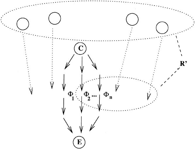
The criterion, illustrated in Figure 4, asserts that causal intervention reveals causal relationships when and only when downstream effects reflect the impact probabilistically. This rules out intransitivity cases, as we want. Note that the issues concerning screening off that vexed early attempts to provide a probabilistic criterion for causality do not even arise: observing I C cuts all other arcs into C, preventing any probabilistic influence from going backwards through a common cause.

Representing perfect intervention on C.

Wiggle Logic I. R fixes a background wherein one or more paths Φi allow intervention on C to make a probabilistic difference.

On the other hand, this formulation fails to cope with accidental neutrality in small worlds: in the neutral Hesslow case, there just is no probabilistic dependency between the pill and thrombosis, because the dual pathways neutralize each other. But this is exactly and only because there are neutralizing multiple pathways. There is no difficulty in extending WL I to cope with multiple paths:
Wiggle Logic II: C causes E with respect to G/R if and only if
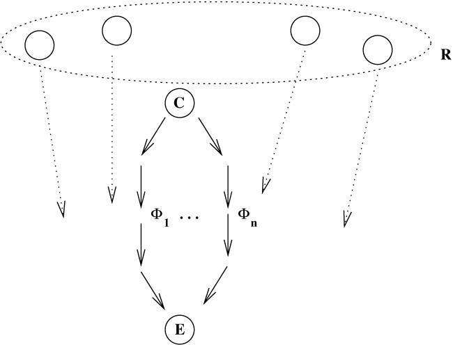
where ∃!Φ ∊ Paths(C, E) means there is a unique directed path Φ from C to E (see Figure 5).

Wiggle Logic II. R ' fixes a background and foreground wherein exactly one path Φi allows an intevention on C to make a probabilistic difference.

The uniqueness requirement for Φ implies that any alternative directed paths from C to E are blocked by R '. The causality criterion, then, just combines transitivity (i.e., there being a directed path) with probabilistic dependence under intervention, but in such a way that any neutralizing alternative pathways are discounted. WL II trivially subsumes WL I; that is, if WL I is satisfied then WL II must be satisfied. For that reason also, any directly linked cause and effect will be identified by WL II.
With this in mind, let us revise CR to talk of restrictions:
Causal Relevance (CR II): C causes E with respect to G/R iff

Clearly if WL II holds, then CR II holds: there is some state of the network such that wiggling C makes a difference to the distribution over E. We conjecture that CR II implies WL II: if the second clause holds without R ' intersecting all but one directed path from C to E, then it also holds under some such circumstance. The advantage of WL II, in any case, lies simply in making the joint dependency on transitive closure and probabilistic dependency explicit.
R identifies the context within which the causality question is raised. R ' identifies some context within which it can be answered. R ' specifies some state of the Bayesian network G as a whole, with all unnamed variables left unobserved and unnamed arcs unrestricted. It may well be that R ' shall need to fix one or more parents of E to particular values before an intervention on C shows any probabilistic impact: that is, it may be that C affects E only in some specific interaction involving other causes. This criterion allows for that.
5.3. Objective Homogeneity
So what about objective homogeneity—or, the model homogeneity which is its representative? In complex worlds, where subjunctive properties are in principle computable beforehand from the rich causal background, objective homogeneity may be enough. However, as we have seen, in simple worlds we need more. Wiggle Logic (and CR) obtain this “more” by reference to any context R ' (or O) in a causal model, homogeneous or not. But in applying these criteria, if we are looking at an inhomogeneous context, we are looking at a wrong context. Suppose, for example, that there is only a single, direct link between C and E. In that case, we can leave
 $R^{\prime }=O$
in WL II, since there are no alternative paths to intercept. But if O fails to specify a homogeneous background, if there are other causes of E that are not held constant, then whether an intervention on C induces a change in the distribution over E may depend upon the prior probability distribution over those unfixed alternative causes. In short, WL II will only provide us with a criterion for belief in causality—even relative to the model at hand, rather than the normative, metaphysical criterion we were after. Without objective homogeneity, WL II is satisfied too easily.
In order to deal with this problem we need to revert to the original idea of OHT, requiring O to be model homogeneous in the first place.Footnote 22 Thus, objective homogeneity refuses to go away.
Because it works thread-by-thread, this forward-looking homogeneity does not allow a direct answer to the question, “What is the overall effect of contraceptive pills on thrombosis?” But then we already knew how to get the right answer to that question: use the traditional computable-beforehand homogeneous reference classes at C. What we answer here is how to determine whether there is in fact some causal relation between C and E—but not what measurable strength that relation has nor how it contributes to an overall impact on E. We leave the proper accounting of the notion of causal strength to future work.
5.4. Simple Simple Worlds
We suggest that WL II provides a fully satisfactory accounting for the neutral thrombosis case. But, it could well be objected that by introducing restriction and control variables we have violated our own assumption of the world being simple: we have added new variables to the model that was supposedly an exhaustive description of the causal world. In short, we have cheated. We unashamedly confess to cheating. Not being permitted this cheat is equivalent to restricting consideration to a world where there is no such thing as causal intervention. But it is arguable that in such a world there is no such thing as causality, and the only legitimate considerations are probabilistic. In that world there is no sense in which the original thrombosis model is superior to the simpler v-structure
 $Pill\rightarrow Pregnancy\leftarrow Thrombosis$
—indeed, there is a sense in which the latter, being a simpler representation of the very same probability structure, is superior. We are not interested in worlds which are non-causal, and our criterion of causality cannot be faulted for failing to find any causality in them.
6. An INUS Condition for Probabilistic Causality
John Mackie (Reference Mackie, Sosa and Tooley1993) proposed the INUS account of causality: that a condition C is a cause of E just in case it is an Insufficient, but Necessary, component of an Unnecessary, but Sufficient, condition for E. This fails, if only because it presupposes a deterministic universe and so rules upon synthetic matters with a priori hubris. What we here offer is quite different, namely an INUS condition for probabilitic causality:
Probabilistic dependency in an objectively homogeneous context is an
Insufficient (in that it requires a causal model to provide the directed chain connecting C and E as well as the parent set of E) but
Necessary part of WL II, which is an
Unnecessary (because of quantum mechanical cases where the Markov property fails), but
Sufficient condition for causality.
7. Conclusion
Unanimity and homogeneity are, of course, related. For one, unanimity is properly defined in terms of homogeneity, as we observed above. But also they both make some attempt to relativize causal claims and avoid the mistake of mixing together distinct effects. Thus, some objections made to relativization apply to both. Those objections succeed, at best, in pointing out that homogeneity theory does not provide much of an account of ordinary causal talk. We shall leave such worries to those who take ordinary language philosophy seriously.
Contextual unanimity theory for probabilistic causality is a red herring: it fails to find the true causal capacities hidden within the mass of artifactual causal claims based upon averages; it also fails to account for ordinary causal talk. Being easily impressed by causal factors that merely push the effect in the same direction, the unanimity account distracts from what is important. It is only from our best estimates of precise causal strengths that we can hope to learn causal structure, as is clearly revealed in the recent literature on causal discovery.
Objective homogeneity, properly understood within a causal context, does not and can not mix distinct causal powers. It handles interactions and allows us to make sense of the learning of causal structure, whether by human or machine. Although causal structure alone does not suffice to identify causality in Bayesian networks (because of intransitivity), causal structure combined with objective homogeneity in Wiggle Logic does.
Finally, Wiggle Logic provides a clear account of the relation between epistemics and metaphysics. Wiggle Logic provides a clear criterion of causal relevance relative to a causal model—just as model homogeneity provides a clear criterion of homogeneity relative to a model (if we replace observations O with restrictions). As we learn more about the world we are in, we refine our causal model of that world, by adding missing nodes and arcs (or, perhaps, deleting some). Our account of causal relevance, and our best guess of what the objectively homogeneous reference classes look like, thereby become more sophisticated. In that way, our model homogeneities may tend toward what are truly the objective homogeneities.
Addendum I: More Pragmatics
We have repeatedly pushed aside ordinary causal talk, except to say that there is an obvious way in which the homogenist does not do violence to ordinary causal talk. But if a homogenist were to estimate the actual risk of smoking for a particular agent, that homogenist would have to specify a reference class. Yet this homogenist would certainly know that the reference class is not truly objectively homogeneous. So, what should we say?
Instead of relying on implicature, one could also give an account of actual causal talk as offering “best recommendations” given an epistemically homogeneous reference class. Such an account might use decision theory to choose the optimal plan given an agent's uncertainty about the homogeneous reference classes. Christopher Hitchcock has developed such an account (Hitchcock Reference Hitchcock2001a, Reference Hitchcock, Kyburg and Thalos2002).Footnote 23 Although his account is presented for a particular agent choosing its own actions, it is easily generalized. This is not our project, but we are sympathetic to such a decision-theoretic approach.
Addendum II: How Objective Homogeneity Is Not Just about Probabilities
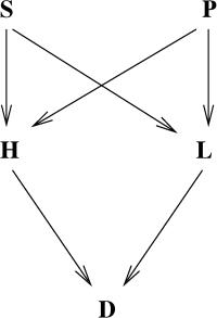
Christopher Hitchcock has asked us why probabilities are the right way to discriminate capacities.Footnote 24 Suppose, he says, there is a population with three different subpopulations, P 1, P 2, and P 3 relevant to smoking S and death D. Smoking always increases the probability of death, but it can do so either via lung cancer L or heart disease H. Smoking increases the probability of death among P 1 and P 2 via H, and among P 3 via L. By strange coincidence it happens, however, that
 $P(D\mid SP_{2}) =P(D\mid SP_{3}) $
, and analogously for ¬S. Hitchcock says, “Then, according to homogeneity, populations P 2 and P 3 should be joined to form one homogeneous sub-population,” which would aggregate different capacities.
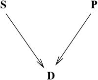
If we model the situation in just the three variables S,P,D, then we have the model shown in Figure 6. In this case, objective homogeneity requires us to combine the populations P 2 and P 3, because of their identical probabilistic consequences for other variables in the model.Footnote 25
Figure 6

But what happens if we decide to model the story as Hitchcock has presented it? In that case our causal model would be as shown in Figure 7. Here we are no longer required to merge the subpopulations of P—rather, we are obliged not to do so, since that would violate the story, misdescribing causal effects on H and L. As its reformulation in WL II makes clear, objective homogeneity discriminates capacities relative to a causal model and not in vacuo. In short, the wrong model leads to wrong conclusions.
Figure 7