2.1 The quaternion group

Consider the real 4-dimensional vector space $\mathbb{H}$ generated by the basis vectors $1$ , $i$ , $j$ , and $k$ . This space is an algebra under the Hamilton product, with $1$ as neutral element, and given on basis elements by $i^2=j^2=k^2=-1$ , $ij=k$ , $ji=-k$ , $jk=i$ , $kj=-i$ , $ki=j$ and $ik=-j$ . The quaternion group is the 8-element group consisting of $1,i,j,k$ and their negatives. This group can easily be shown to admit the presentation

(1) \begin{equation} Q=\left \langle e,i,j,k\ \middle |\ i^2=e,j^2=e,k^2=e,ijk=e,e^2=1\right \rangle \end{equation}

where $e$ denotes $-1$ . The following alternative presentation will prove useful later in the paper.

Lemma 1. The quaternion group admits the presentation

(2) \begin{equation} Q= \langle i,j\ |\ i=jij,j=iji \rangle \end{equation}

Proof. We first show that the group admits the presentation

(3) \begin{equation} Q=\left \langle i,j\ \middle |\ i^4=1,i^2=j^2,iji=j\right \rangle \end{equation}

We have the following equivalent presentations:

\begin{align*}\begin{array}{l@{\quad}l} Q=\left \langle e,i,j,k\ \middle |\ i^2=e,j^2=e,k^2=e,ijk=e,e^2=1\right \rangle& \\[5pt] Q=\left \langle i,j,k\ \middle |\ j^2=i^2,k^2=i^2,ijk=i^2,i^4=1\right \rangle& \;\;\text{using $e=i^2$}\end{array} \end{align*}

In the second presentation above, $ij=k$ is derivable because we have $ijk=i^2$ , multiplying by $k^3$ yields $ijk^4=i^2k^3$ , and therefore, $ij=k$ since $k^4=i^4=1$ and $i^2k^2=i^4=1$ . We thus have the following presentations:

\begin{align*} \begin{array}{l@{\quad}l} Q=\left \langle i,j,k\ \middle |\ j^2=i^2,k^2=i^2,ijk=i^2,i^4=1,ij=k\right \rangle & \\[5pt] Q=\left \langle i,j\ \middle |\ j^2=i^2,(ij)^2=i^2,ijij=i^2,i^4=1\right \rangle &\;\; \text{using $k=ij$} \end{array} \end{align*}

The relation $(ij)^2=i^2$ is now redundant, so that we can remove it, and then, from the relation $ijij=i^2=j^2$ , we can derive the equivalent relation $iji=j$ by dividing by $j$ , and we obtain (3):

\begin{align*} Q&=\left \langle i,j\ \left |\ i^4=1,i^2=j^2,iji=j\right .\right \rangle \end{align*}

We can now show that the presentation (3) is equivalent to (2). From (3), we can derive the missing relation $i=jij$ by

\begin{align*} \begin{array}{ll@{\quad}l} jij&=iji^2j &\text{by}\;j=iji\\[-2pt] &=ij^4& \text{by}\;i^2=j^2\\[-2pt] &=i& \text{by}\;j^4=i^4=1 \end{array} \end{align*}

Conversely, from (2), we can derive the relations of (3) since $i^2=jiji=j^2$ , and $j=iji=jij^2i=ji^4$ , which implies $1=i^4$ by division by $j$ .

2.2 The hypercubical manifold

We write $C=\left \{t1+xi+yj+zk\ \middle |\ t,x,y,z\in [-1,1]\right \}\subseteq \mathbb{H}$ for the unit cube in $\mathbb{H}$ and $\partial C\subseteq C$ for its boundary (consisting of the points such that at least one of the coordinates is either $-1$ or $1$ ). Note that $\partial C$ is homotopy equivalent to the 3-sphere $\operatorname {S}^{3}$ . There is a natural action of $Q$ on $C$ by left multiplication. This action is not free since it fixes $0$ , but it becomes free when restricted to $\partial C$ . We write

\begin{equation*} K \equiv \partial C/Q \end{equation*}

for the quotient space of $\partial C\simeq \operatorname {S}^{3}$ under this action and refer to it as the hypercubical manifold. It is not immediately clear from this description that $K$ is actually a manifold (as opposed to a topological space), but this will not play a role here. Because the action is free and properly discontinuous as $Q$ is finite, the quotient map $\partial C\to K$ is covering with fiber $Q$ (Hatcher Reference Hatcher2009, Proposition 1.40); that is, we have a fiber sequence

\begin{equation*} Q\longrightarrow \partial C\longrightarrow K \end{equation*}

from which we deduce that the fundamental group of $K$ is $Q$ (Hatcher Reference Hatcher2009, Theorem 4.41).

The original definition of $K$ (Poincaré Reference Poincaré1895, p. 66, Section 13, troisième exemple) is quite different in nature, with the equivalence explained in de Saint Gervais (Reference de Saint Gervais2022). Indeed, the hypercubical manifold can alternatively be described as a 3-dimensional cube, whose opposite faces are identified after a quarter-turn rotation:

(4)

Hence $K$ can be represented as a CW-complex with two 0-cells ( $a$ and $b$ ), four 1-cells ( $x$ , $y$ , $z$ and $w$ ), three 2-cells ( $\alpha$ , $\beta$ , and $\gamma$ , corresponding to the front, right, and top faces),

(5)

and one 3-cell ( $A$ , representing the interior of the cube). This definition allows for a direct computation of the fundamental group $\pi _1(K)$ . We first contract $w$ to an identity (thus identifying $a$ and $b$ ) to obtain the presentation

\begin{equation*} \pi _1(K) = \langle x,y,z\ |\ x=zy,y=xz,z=yx \rangle \end{equation*}

where the three relations correspond to the 2-cells (5). By removing $z$ (which is equal to $yx$ ), renaming $x$ to $i$ and $y$ to $j$ , we recover the presentation of Lemma1 of the quaternion group.

2.3 Higher hypercubical manifolds

We now briefly discuss higher-dimensional generalizations of the hypercubical manifold. These arise quite naturally from our work, but to the best of our knowledge, have not been previously considered in the literature. Writing $K^{1}$ for the hypercubical manifold, we observe that $K^{1}$ is a “good approximation” of $Q$ up to dimension $2$ , in the sense that we have

\begin{align*} \pi _0(K^{1})=\pi _0(\!\operatorname {B} Q)=1 \qquad \pi _1(K^{1})=\pi _1(\!\operatorname {B} Q)=Q \qquad \pi _2(K^{1})=\pi _2(\!\operatorname {B} Q)=1 \end{align*}

More generally, we would like to have cellular spaces $K^{n}$ , which coincide with $Q$ up to dimension $f(n)$ , where $f$ is a strictly increasing function on the natural numbers, thus constructing a resolution of $Q$ . In fact, the construction of $K^{1}$ generalizes as follows.

Given $n\in \mathbb{N}$ , we can consider the unit cube $C^n\subseteq \mathbb{H}^n$ . We write $\partial C^n$ for its boundary, which is homotopy equivalent to the $(4n{-}1)$ -sphere $\operatorname {S}^{4n-1}$ . As before, we have an action of $Q$ on $C^n$ , which restricts to a free action on $\operatorname {S}^{4n-1}$ : we have that $\operatorname {S}^{4n-1}$ can be expressed as the join of $n$ copies of $\operatorname {S}^{3}$ , and $Q$ acts independently on each of these 3-spheres, as explained in the previous section. We define

\begin{equation*} K^{n} \equiv \operatorname {S}^{4n-1}\!\!/Q \end{equation*}

as the quotient of the sphere under this action. By Hatcher (Reference Hatcher2009, Proposition 1.40), we thus have the fiber sequence

\begin{equation*} Q\longrightarrow \operatorname {S}^{4n-1}\longrightarrow K^{n}\end{equation*}

which simply encodes the fact that the map on the right has $Q$ as fibers, from which we deduce that $\pi _i(K^{n})=\pi _i(\!\operatorname {B} Q)$ for $0\leq i\leq 4n-2$ , using the induced long exact sequence in homotopy (Hatcher Reference Hatcher2009, Theorem 4.41).

There is a canonical inclusion $\mathbb{H}^n\to \mathbb{H}^{n+1}$ (obtained by adding $0$ as last coordinate) which induces an inclusion $\partial C^n\to \partial C^{n+1}$ , and thus a map $K^{n}\to K^{n+1}$ . Taking the inductive limit yields a space $K^{\infty }$ which has the same homotopy groups as $\operatorname {B} Q$ (because homotopy groups commute with inductive limits (May Reference May1999, Chapter 9, Section 4)) and is thus homotopy equivalent to $\operatorname {B} Q$ (Hatcher Reference Hatcher2009, Theorem 1B.8). However, this model has the advantage of being a CW-complex which can be explicitly described.

Again, all the constructions above are very “classical” in nature, in the sense that we use strict quotients of spaces, boundaries of spaces, and so on. We will see in the rest of the paper how to perform them in a homotopy-invariant way, so that they can be formalized in homotopy type theory.

3.1 Elementary constructions

We denote by $\mathscr{U}$ the universe of all types (strictly speaking, one should assume a hierarchy of universes, but we will not detail this as it plays no essential role here). Given a type $A:\mathscr{U}$ and a type family $B:A\to \mathscr{U}$ , we write $\Pi A.B$ , or $\Pi (x:A).B\,x$ , or $(x:A)\to B\,x$ for the associated dependent product type: its inhabitants are dependent functions, and we write $\lambda x.t$ for the function that associates to $x$ (of type $A$ ) the term $t$ (of type $B\,x$ ). As usual, we write $A\to B$ for the type of non-dependent functions (here, we suppose that $B$ is a non-dependent type). Similarly, we write $\Sigma A.B$ or $\Sigma (x:A).B\,x$ for the type of dependent sums, whose elements are dependent pairs $\langle t,u\rangle$ consisting of a term $t$ (of type $A$ ) and a term $u$ (of type $Bt$ ). The two dependent projections are, respectively, written $\operatorname {fst}:\Sigma A.B\to A$ and $\operatorname {snd}:(x:\Sigma A.B)\to B\,(\!\operatorname{fst} x)$ . Given two type families $B:A\to \mathscr{U}$ and $B':A'\to \mathscr{U}$ , and maps $f:A\to A'$ and $g:(x:A)\to B\,x\to B'\,(f\,x)$ , we write $\Sigma f.g:\Sigma A.B\to \Sigma A'.B'$ for the canonically induced map. Given a natural number $n$ , we still write $n$ for the type with $n$ elements and even occasionally use the comprehension notation such as $\left \{a,b,c\right \}$ to denote the type $3$ , where the three elements are called $a$ , $b$ , and $c$ . In particular, we denote by $0$ (resp. $1$ ) the initial (resp. terminal) type.

We write $t\equiv u$ to indicate that two terms $t$ and $u$ are definitionally equal. Homotopy type theory also provides, for all elements $t$ and $u$ of common type $A$ , a type $t=u$ of propositional equalities (or identities) between $t$ and $u$ , also called paths because of their topological interpretation. We write $\operatorname {refl}_{x}:x=x$ for the trivial path on a point $x:A$ . Given paths $p:x=y$ and $q:y=z$ , we write $p\cdot q:x=z$ for the path obtained by concatenation and $\overline p:y=x$ for the inverse of $p$ . Given an identity $p:A=B$ between types $A$ and $B$ , we write $p^\to :A\to B$ for the canonical function induced by transport (Univalent Foundations Program 2013, Lemma 2.3.1). Given a function $f:A\to B$ and a path $p:t=u$ in $A$ , we write $f^=(p):f(t)=f(u)$ (or even sometimes $f(p)$ ) for the canonical path in $B$ (Univalent Foundations Program 2013, Lemma 2.2.1), which can be thought of as being obtained by applying $f$ pointwise to $p$ . All constructions in homotopy type theory are compatible with identities; in particular, all (co)limits are taken up to homotopy.

A pointed type consists of a type $A$ together with an element of $A$ , which we often denote by $\star$ , and a pointed map is a function preserving the distinguished element. Given a pointed type $A$ , we write $\operatorname {\Omega } A\equiv (\!\star =\star )$ for the loop space of $A$ .

Given a type $A$ , we write $\|A\|_{-1}$ (resp. $\|{A}\|_{0}$ , resp. $\|A\|_{1}$ ) for its propositional (resp. set, resp. groupoid) truncation and $|-|_{n}:A\to \|A\|_{n}$ for the canonical quotient map. In fact, the $n$ -truncation $\|A\|_{n}$ of $A$ can be defined for any natural number $n$ , and we say that $A$ is $n$ -connected when $\|A\|_{n}$ is contractible, and we sometimes simply say connected for a $0$ -connected type. By extension, a map $f:A\to B$ is $n$ -connected when the homotopy fiber $\operatorname {fib}_{f}y$ (defined below) is $n$ -connected for every $y:B$ .

3.2 Fibrations

Any type family $F:A\to \mathscr{U}$ can be thought of as a fibration with $A$ as base space, whose fiber at $x:A$ is simply $F\,x$ . The total space of such a fibration is $\Sigma A.F$ , which comes equipped with a projection map

\begin{equation*} \operatorname {fst}:\Sigma A.F\to A \end{equation*}

onto the base space given by the first projection. Conversely, any map $f:X\to A$ (exhibiting $X$ as a type over $A$ ) induces a type family $\operatorname {fib}_{f}:A\to \mathscr{U}$ , which associates to each element $y:A$ its homotopy fiber defined as

\begin{equation*} \operatorname {fib}_{f} y \equiv \Sigma (x:X).(y=f\,x) \end{equation*}

which corresponds to the pullback

These constructions provide an equivalence between the two perspectives on fibrations, as type families indexed by $A$ or as types over $A$ . This is known as the Grothendieck duality (Univalent Foundations Program 2013, Theorem 4.8.3):

Proposition 2 (Grothendieck duality). For any type $A:\mathscr{U}$ , we have an equivalence between type families and types over $A$

\begin{equation*} (A \to \mathscr{U}) \simeq (\Sigma (B:\mathscr{U}).B \to A) \end{equation*}

We say that a pair of composable maps

with $A$ pointed, is a fiber sequence when $F=\operatorname {fib}_{f}\star$ and $i$ is the canonical map given by the above pullback. This indicates that $f$ can be regarded as a fibration whose fibers are all $F$ (when $A$ is connected, all the fibers are indeed merely equivalent to $F$ ). Fiber sequences play a role analogous to short exact sequences in abelian categories.

For reasons indicated above, given a type family $F:A\to \mathscr{U}$ , it is often desirable to compute its total space $\Sigma A.F$ . When $A$ is constructed as a colimit (such as a coequalizer or a pushout), this total space can also be obtained as a similar colimit: this is called the flattening lemma. For pushouts, which is the variant we will use here, this fact can be formulated as follows (Univalent Foundations Program 2013, Lemma 8.5.3):

Lemma 3 (Flattening lemma for pushouts). Consider a pushout square

with $p:(x:X)\to (i\circ f)(x)=(j\circ g)(x)$ witnessing its commutativity and a type family

\begin{equation*} F:A\sqcup _XB\to \mathscr{U}\end{equation*}

The following square of total spaces is also a pushout:

where

\begin{align*} e:(x:X)\to (F\circ i\circ f)(x)&\to (F\circ j\circ g)(x)\\ x\,y&\mapsto (F^=(p\,x))^\to \,y \end{align*}

is the map canonically induced by $p$ .

A similar result holds when $A$ is constructed as a coequalizer (Univalent Foundations Program 2013, Lemma 6.12.2).

3.3 Groups and actions

A group $G$ is a set together with a multiplication and unit satisfying the usual axioms. A delooping of $G$ is a pointed connected space $\operatorname {B} G$ together with an isomorphism of groups $\operatorname {\Omega }\operatorname {B} G\simeq G$ (where the group structure on $\operatorname {\Omega }\operatorname {B} G$ is the one induced by concatenation of paths). A type with this property can be shown to exist and be unique (Wärn Reference Wärn2023), so that we can talk about the delooping of a group. In fact, the loop space provides an equivalence between pointed connected groupoids and groups (Bezem et al. Reference Bezem, Buchholtz, Cagne, Dundas and Grayson2026). This equivalence implies in particular that we have the following recursion principle:

A map $\phi :\operatorname {B} G\to \mathscr{U}$ can be interpreted as an action of $G$ on the type $X\equiv \phi (\!\star\!)$ . Indeed, any $a\in G$ corresponds to a path $a:\star =\star$ in $\operatorname {B} G$ and, thus induces, by transport, an endomorphism $(\phi ^= a)^\to :X\to X$ . In the case where $X$ is a set, this can be shown to correspond to the traditional notion of action. More generally, a map $\operatorname {B} G\to \mathscr{U}$ can be thought of as an action of $G$ on a higher type in a coherent way. With this point of view, the homotopy quotient of $X$ by $G$ is the type $X{/\!\!/} G\equiv \Sigma (\!\operatorname {B} G).\phi$ . The Grothendieck duality (Proposition2), which states that the type of maps $A\to \operatorname {B} G$ is equivalent to the type of families $\operatorname {B} G\to \mathscr{U}$ , can thus be read as the following equivalence, which we call the action-fibration duality:

Proposition 5. A fiber sequence

corresponds to a coherent action of $G$ on $X$ (i.e., a map $\phi :\operatorname {B} G\to \mathscr{U}$ with $\phi (\!\star\!)=X$ ) with $A$ being the homotopy quotient $X{/\!\!/} G$ .

In the above proposition, the action is obtained as the map $\operatorname {fib}_{f}:\operatorname {B} G\to \mathscr{U}$ , whose total space is $A=\Sigma (\!\operatorname {B} G).\operatorname {fib}_{f}$ , which is, by definition, the homotopy quotient of $X$ by the action of $G$ .

4.1 The hypercubical manifold

We are now ready to define the type that will play a central role in what follows:

We will see in Proposition11 that the fundamental group of $K$ is $Q$ . This is expected from the topological constructions (see Subsection 2.2), but showing this directly is not easy (although it should be doable using the Seifert–van Kampen theorem (Univalent Foundations Program 2013, Section 8.7)).

4.2 Definition of the action

We now define the map $\phi :K \to \operatorname {B} Q$ . To motivate its definition, we can start from the computation of Subsection 2.2, which identifies the fundamental group of $K$ with $Q$ (an alternative and more abstract starting point will also be given in Subsection 4.8). We see that the path $x$ corresponds to $i$ , the path $y$ corresponds to $j$ , the relation $z=yx$ imposes that $z$ should correspond to $ji=-k$ , and the path $w$ was contracted and should thus correspond to $1$ . This suggests the following definition of the map $\phi$ , using the elimination principle of $K$ .

Definition 8. We define a morphism $\phi :K \to \operatorname {B} Q$ on 0-cells by

\begin{equation*} \phi (a)\equiv \phi (b)\equiv \star {} \end{equation*}

and on 1-cells by

\begin{align*} \phi (x)\equiv i \qquad \phi (y)\equiv j \qquad \phi (z)\equiv -k \qquad \phi (w)&\equiv 1 \end{align*}

The 2-cells are sent to 2-cells coming from the following relations, which are known to hold in $Q$ :

\begin{align*} \phi (\alpha ):i=jk \qquad \phi (\beta ):j=ki \qquad \phi (\gamma )&:k=ij \end{align*}

On 3-cells, $\phi$ is unambiguously defined because $\operatorname {B} Q$ is a groupoid.

For $k\in \mathbb{N}$ , we define $K^{k}$ to be the $k$ -skeleton of $K$ ; that is, $K^{k}$ is defined as the HIT generated by the same $i$ -cells for $i\leq k$ (and none for $i\gt k$ ). We write $\phi _k:K^{k}\to \operatorname {B} Q$ for the composite map 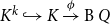$K^{k}\hookrightarrow K \xrightarrow {\phi }\operatorname {B} Q$ . Our goal is now to compute the (homotopy) fiber $\operatorname {fib}_{\phi _k}$ , by induction on $k$ , using the flattening lemma, and ultimately show that $\operatorname {fib}_{\phi }\equiv \operatorname {fib}_{\phi _3}=\operatorname {S}^{3}$ in Theorem 4.7.

4.3 Fiber of the 0-skeleton

The 0-skeleton $K^{0}$ is a space consisting of two points $a$ and $b$ , and the induced map $\phi _0:K^{0}\to \operatorname {B} Q$ is the constant map with $\star {}$ as image. Its fiber is

\begin{align*} \operatorname {fib}_{\phi _0} &\equiv \Sigma (x:K^{0}).(\!\star {}=\phi _0(x)) \\ &= (\!\star {}=\phi (a)) \sqcup (\!\star {}=\phi (b)) \\ &= \left \{a,b\right \}\times (\!\star {}=\star {}) \\ &= \left \{a,b\right \}\times Q \end{align*}

so that we have a fiber sequence

4.4 Fiber of the 1-skeleton

The 1-skeleton $K^{1}$ is that of the complex pictured in (4), with two 0-cells $a$ and $b$ and four 1-cells $x$ , $y$ , $z$ , and $w$ . It can be obtained from $K^{0}$ as the coequalizer

where the maps $\sigma$ and $\tau$ , respectively, send an edge to its source and target; that is, they are the constant maps, respectively, equal to $a$ and $b$ .

Our aim is now to compute the fiber of $\phi _1:K^{1}\to \operatorname {B} Q$ . We consider the type family

\begin{align*} F_1:K^{1}&\to \mathscr{U}\\ x&\mapsto (\!\star {}=\phi _1(x)) \end{align*}

This family is defined so that we have

\begin{equation*} \operatorname {fib}_{\phi _1}\equiv \Sigma (x:K^{1}).F_1(x) \end{equation*}

which can be computed using the flattening lemma for coequalizers (see Proposition 2 and Univalent Foundations Program (2013, Section 6.12)) to be the coequalizer

(6)

where $e$ is defined as

\begin{align*} e:(p:\{x,y,z,w\})\to (F_1\circ \iota _1\circ \sigma )(p)&\to (F_1\circ \iota _1\circ \tau )(p)\\ p\ q&\mapsto (F_1^=\,p)^\to \,q \end{align*}

(note that, above, both types $(F_1\circ \iota _1\circ \sigma )(p)$ and $(F_1\circ \iota _1\circ \tau )(p)$ are equal to $\operatorname {\Omega }\operatorname {B} Q$ ). We have $F_1(\iota _1(\sigma (x)))\equiv (\!\star {}=\star {})=Q$ and similarly for $y$ , $z$ , and $w$ , so that (6) can be rewritten as

(7)

By properties of transport in path types (Univalent Foundations Program 2013, Theorem 2.11.4), we thus have $e\,p\,q=q\cdot \phi ^=\,p$ . Equivalently, in (7), we can thus define

\begin{align*} e:\{x,y,z,w\}&\to Q\to Q\\ p\ q&\mapsto q\cdot \phi ^=(p) \end{align*}

by slightly overloading $e$ , where $\cdot$ denotes the multiplication in $Q$ , and we implicitly identify $\phi ^=(p)$ , which is an element of $\operatorname {\Omega }\operatorname {B} Q$ with the corresponding element of $Q$ .

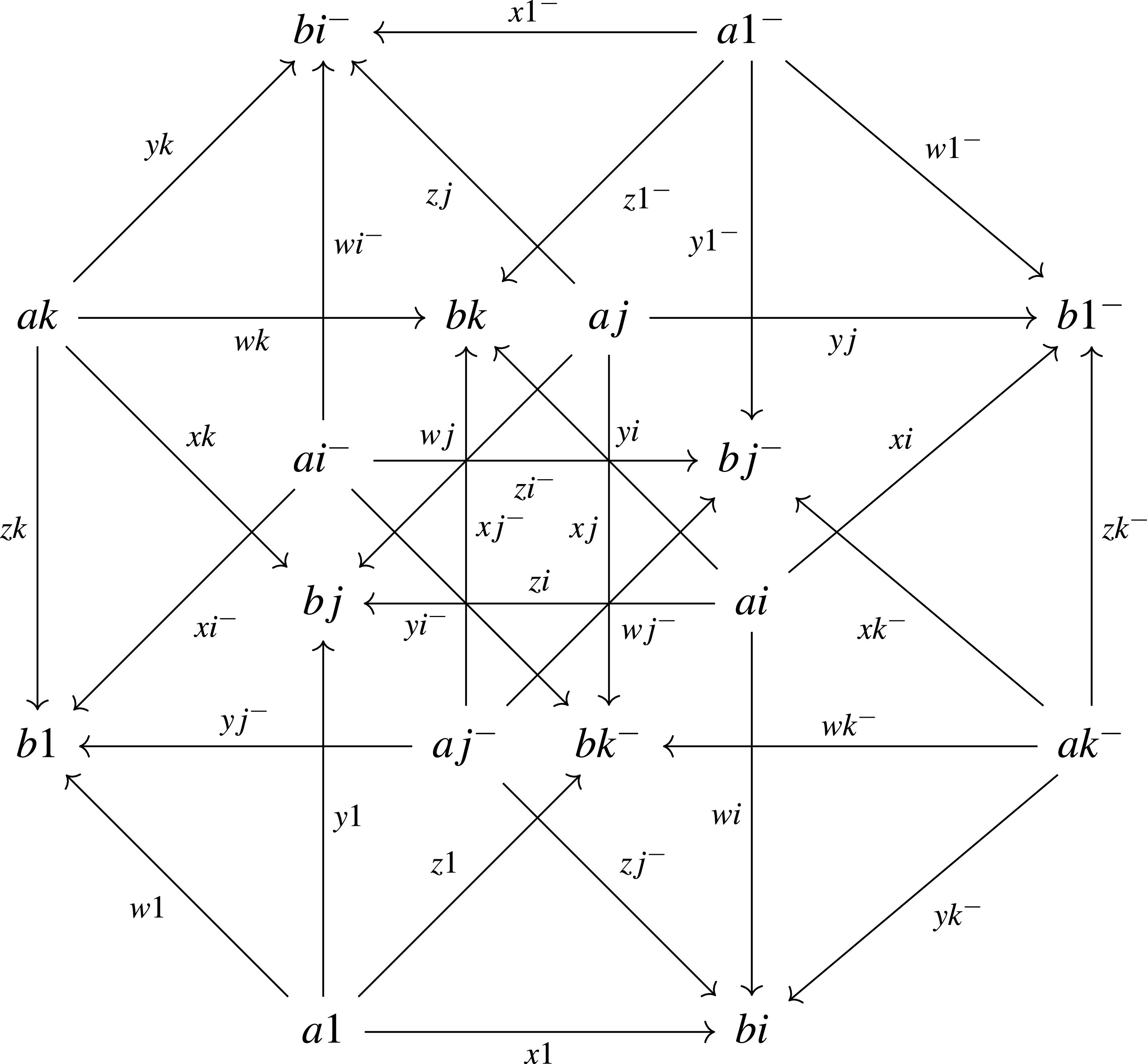
The coequalizer (7) can be interpreted as a description of $\operatorname {fib}_{\phi _1}$ as a 1-dimensional cell complex, with $K^{0}\equiv \{a,b\}\times Q$ as 0-cells and $\{x,y,z,w\}\times Q$ as 1-cells, the source and target of a 1-cell $(p,q):\{x,y,z,w\}\times Q$ being, respectively, $(a,q)$ and $(b,q\cdot \phi ^=(p))$ . This complex is pictured in Figure 1. Here, we write $ai$ (resp. $ai^-$ ) for $(a,i)$ (resp. $(a,-i)$ ) and similarly for other cells, so that the general form of a 1-cell is

We can observe that this is the 1-skeleton of a tesseract (a 4-dimensional cube), which is homotopic to $\operatorname {S}^{3}$ as expected.

Figure 1.

The fiber of $\phi _1$ (the 1-skeleton of a cubical model of $\operatorname {S}^{3}$ ).

Figure 1. Long description

A diagram representing the fiber of the 1-skeleton of a cubical model. The diagram features a complex network of labeled points and lines, illustrating the relationships and connections between different components. Key labeled points include ai, aj, ak, bi, bj, bk, b1, a1, wi, wj, wk, xi, xj, xk, yi, yj, yk, zi, zj, and zk. The lines connecting these points indicate the structure and flow within the model, with arrows showing the direction of relationships. The overall structure is symmetrical and interconnected, highlighting the intricate nature of the fiber in the 1-skeleton of a cubical model.

Figure 2.

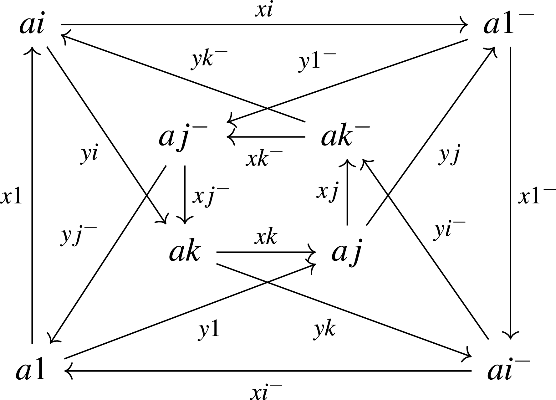
Cayley graph of $Q$ generated by $i$ and $j$ .

Remark 9. The group $Q$ is generated by $i$ and $j$ , and so, it admits the Cayley graph $C$ shown in Figure 2. This graph describes a HIT (with the vertices as generators and edges as identities), which can be obtained as the fiber of the canonical map $\operatorname {B}\{i,j\}^*\to \operatorname {B} Q$ , where $\{i,j\}^*$ is the free group on two generators (see Champin et al. Reference Champin, Mimram and Oleon2024, Theorem 16). Similarly, we have a Cayley graph $C'$ associated to $\{x,y,z\}$ as generators (where $x$ , $y$ , and $z$ , respectively, correspond to $i$ , $j$ , and $-k$ ). We have a map $f:K^{1}\to \operatorname {B}\{x,y,z\}^*$ , which expresses that the target can be obtained from the source by contracting the 1-cell $w$ to a point, that is,

\begin{align*} f(a)\equiv \star \qquad f(b)\equiv \star \qquad f(x)\equiv x \qquad f(y)\equiv y \qquad f(z)\equiv z \qquad f(w)\equiv \operatorname {refl}_{\star } \end{align*}

We also have a map $g:\operatorname {B}\{i,j\}^*\to \operatorname {B}\{x,y,z\}^*$ , which is the canonical inclusion of cells, respectively, sending $x$ and $y$ to $i$ and $j$ . These maps make the two triangles on the right commute:

where $\twoheadrightarrow$ (resp. $\hookrightarrow$ ) indicates a map which is surjective (resp. injective) on loop spaces. In other words, these maps express that $\operatorname {B}\{i,j\}^*$ can be obtained as a “subquotient” of $K^{1}$ (quotienting by $w$ and forgetting $z$ ). By the universal property of $C'$ , which is a fiber, we have similar maps $f'$ and $g'$ as shown above between the fibers, expressing that $C$ can be obtained as a subquotient of $\operatorname {fib}_{\phi _1}$ , by quotienting all 1-cells of the form $(w,q)$ with $q\in Q$ (and thus identifying all 0-cells $(b,q)$ with $(a,q)$ ) and forgetting all the 1-cells of the form $(z,q)$ with $q\in Q$ . It can be checked that if we perform these operations on $K^{1}$ pictured in Figure 1, we recover the traditional Cayley graph pictured in Figure 2.

4.5 Fiber of the 2-skeleton

We write $\square$ for the HIT corresponding to an empty square, generated by four 0-cells $v_0,v_1,v_2,v_3$ and four 1-cells $e_0,e_1,e_2,e_3$ attached as in the following picture:

We also write for the HIT corresponding to a filled square, obtained from the previous one by attaching a 2-cell as expected. There is an induced canonical inclusion The type is contractible, and we will consider a particular equivalence consisting of the terminal map and the map pointing at $v_0$ . Since these form an equivalence, their composite is the identity on , which is witnessed by a homotopy Up to deformation (being an equivalence is a property), we can consider a particular definition for $\varepsilon$ , which is obtained by induction on , and satisfies

\begin{align*} \varepsilon (v_0)\equiv \operatorname {refl} \qquad \varepsilon (v_1)\equiv e_0 \qquad \varepsilon (v_2)\equiv e_1 \qquad \varepsilon (v_3)&\equiv e_0\cdot \overline {e_2} \end{align*}

definitionally (on 1- and 2-cells, this is defined arbitrarily, using the fact that the filled square is contractible). This will slightly simplify subsequent computations.

The 2-skeleton $K^{2}$ can be obtained from $K^{1}$ as the pushout on the left

where the vertical map $\psi$ sends each formal cell to its boundary, as pictured in (5), and the horizontal map $\iota$ is the identity on the first component and the canonical inclusion of the boundary of the square. We write $\tilde h:\tilde \rho \circ \iota =\iota _2\circ \psi$ for the canonical homotopy witnessing the commutativity of the square. By composing the upper-right corner with the equivalence described above, we obtain the pushout figured on the right above, where $\operatorname {fst}:\{\alpha ,\beta ,\gamma\}\times \square \to \{\alpha ,\beta ,\gamma \}$ is the first projection $\operatorname {fst}\equiv (\!\operatorname {id}_{\{\alpha ,\beta ,\gamma \}}\times \tau )\circ \iota$ and $\rho :\{\alpha ,\beta ,\gamma \}\to K^{2}$ , defined as $\rho \equiv \tilde \rho \circ (\!\operatorname {id}_{\{\alpha ,\beta ,\gamma \}}\times \upsilon )$ sends $\alpha$ to the corner of the square $\alpha$ in $K^{2}$ , corresponding to $v_0$ , that is, $a$ (and similarly for $\beta$ and $\gamma$ ). Hence, $\rho$ is the constant map equal to $a$ . More interestingly, the family of equalities $\tilde h$ is transformed into the family $h:\rho \circ \operatorname {fst}=\iota _2\circ \psi$ obtained as the composite $h=\tilde \varepsilon \cdot \tilde h$ where $\tilde \varepsilon :\rho \circ \operatorname {fst}\equiv \tilde \rho \circ (\!\operatorname {id}_{\{\alpha ,\beta ,\gamma \}}\times (\upsilon \circ \tau ))\circ \iota =\tilde \rho \circ \iota$ is the equality canonically induced by $\varepsilon$ .

As previously, we consider the type family $F_2:K^{2}\to \mathscr{U}$ defined by

\begin{equation*} F_2(x) \equiv (\!\star {}=\phi _2(x)) \end{equation*}

The flattening lemma for pushouts (Lemma3) ensures that $\Sigma K^{2}.F_2$ can be computed as the pushout

(8)

The morphism

\begin{equation*} E:((\omega ,s):\{\alpha ,\beta ,\gamma \}\times \square )\to (F_2\circ \rho \circ \operatorname {fst})(\omega ,s)\to (F_2\circ \iota _2\circ \psi )(\omega ,s) \end{equation*}

is defined as follows on $(\omega ,s):\{\alpha ,\beta ,\gamma \}\times \square$ . We have a path

\begin{equation*} h(\omega ,s):(\rho \circ \operatorname {fst})(\omega ,s)=(\iota _2\circ \psi )(\omega ,s) \end{equation*}

which, by applying $F_2$ , induces a path

\begin{equation*} F^=_2(h(\omega ,s)):(F_2\circ \rho \circ \operatorname {fst})(\omega ,s)=(F_2\circ \iota _2\circ \psi )(\omega ,s) \end{equation*}

which, by transport, induces the desired map

\begin{equation*} (F^=_2(h(\omega ,s)))^\to :(F_2\circ \rho \circ \operatorname {fst})(\omega ,s)\to (F_2\circ \iota _2\circ \psi )(\omega ,s) \end{equation*}

Now, observe that for any $\omega :\{\alpha ,\beta ,\gamma \}$ , we have

\begin{equation*} (F_2\circ \rho )(\omega ) = F_2(a) = (\!\star = \phi _2(a)) = (\!\star =\star ) = Q \end{equation*}

because $\rho$ is the constant map at $a : K^{2}$ , and thus, the upper-right corner of the pushout (8) is

\begin{equation*} \Sigma (\omega :\{\alpha ,\beta ,\gamma \}).(F_2\circ \rho )(\omega ) = \{\alpha ,\beta ,\gamma \} \times Q \end{equation*}

the upper-left corner can be transformed similarly as $\Sigma (\{\alpha ,\beta ,\gamma \}\times \square ).Q$ , which is equivalent to $\{\alpha ,\beta ,\gamma \}\times Q\times \square$ . Finally, the lower left corner

\begin{equation*} \Sigma K^{1}.(F_2\circ \iota _2) \equiv \Sigma K^{1}.F_1 \end{equation*}

is precisely the fiber $\operatorname {fib}_{\phi _1}$ computed in the previous section. The pushout (8) can thus be slightly simplified as the pushout

The map $\tilde \psi$ is defined, for $\omega :\{\alpha ,\beta ,\gamma \}$ , $q:Q$ and $s:\square$ , by

\begin{equation*} \tilde \psi (\omega ,q,s) = (\psi (\omega ,s),(F^=_2(e(\omega ,s)))^\to \,q) = (\psi (\omega ,s),q\cdot \phi ^=_2(e(\omega ,s))) \end{equation*}

The values of this map can be computed explicitly. We fix $\omega \equiv \alpha$ (computing the images for $\beta$ and $\gamma$ is similar) and compute the image depending on $s$ . When $s$ is a vertex, we have:

• • for $v_0$ , the image is $(a,q)$ ,

• • for $v_1$ , the image is $(b,q\cdot \phi _2(x))\equiv (b,q\cdot i)$ because $x$ is the path in $\alpha$ corresponding to $e_0\equiv \varepsilon (v_1)$ ,

• • for $v_2$ , the image is $(b,q\cdot \phi _2(y))\equiv (b,q\cdot j)$ because $y$ is the path in $\alpha$ corresponding to $e_1\equiv \varepsilon (v_2)$ ,

• • for $v_3$ , the image is $(a,q\cdot \phi _2(x)\cdot \phi _2(\overline w))\equiv (a,q\cdot i)$ because $x\cdot \overline w$ is the path in $\alpha$ corresponding to $e_0\cdot \overline {e_2}\equiv \varepsilon (v_3)$ .

The image of an edge $e_i:v_j\to v_k$ is the edge whose first component is the edge in $\alpha$ corresponding to $e_i$ and the second component is the element of $Q$ corresponding to the first component of the image of its source $v_j$ . The squares $\alpha$ , $\beta$ , and $\gamma$ are thus, respectively, sent to the following squares in $\operatorname {fib}_{\phi _1}$ :

and

We, respectively, write $(\alpha ,q)$ , $(\beta ,q)$ , and $(\gamma ,q)$ for these cells. Finally, the previous pushout states that $\operatorname {fib}_{\phi _2}$ can be obtained from $\operatorname {fib}_{\phi _1}$ by attaching cells along these boundaries for any $q:Q$ .

4.6 Fiber of the 3-skeleton

The computation of the 3-skeleton can be performed similarly, as we now explain (with fewer details, the computations being similar). We write for the standard cube, which is the HIT pictured on the left

we also write for the variant with a 3-cell filling the interior of the cube. We have a map 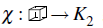sending the standard cube (on the left) to the expected cube in $K^{2}$ (on the right above), where $\alpha$ , $\beta$ , and $\gamma$ are, respectively, the front, right, and top faces of the cube. The type $K$ can be obtained as the pushout on the left:

Since the type is contractible, the pushout is equivalent to the one on the right, where the right vertical map is pointing to $a$ (the image of $v_{---}$ ).

Consider the type family $F:K \to \mathscr{U}$ defined by $F(x)\equiv (\!\star {}=\phi (x))$ . By the flattening lemma for pushouts, we have a pushout as on the left, which can equivalently be computed as on the right:

thus, we have an explicit construction of $\operatorname {fib}_{\phi }$ . The map $\tilde \chi$ can be computed in a similar way to the above and sends, for $q:Q$ , the cube to

Finally, this provides us with a description of $\operatorname {fib}_{\phi }$ as a HIT consisting of cubical cells (16 0-cells, 32 1-cells, 24 2-cells, 8 3-cells) which can easily be checked to form an empty 4-cube, which is homotopy equivalent to $\operatorname {S}^{3}$ . We have also provided a computer-checked formalization of this result, consisting of an explicit construction of the equivalence between the above HIT and the standard tesseract in the proof assistant Agda (Mimram and Oleon Reference Mimram and Oleon2025). In the future, it would be interesting to perform a complete formalization of the above computations, although this is expected to be a considerable amount of work.

4.7 The fundamental fiber sequence

The previous computation can be summarized by the following fiber sequence.

Theorem. We have a fiber sequence

that we call the $\text{fundamental fiber sequence}$ , which encodes a coherent action of $Q$ on $\operatorname {S}^{3}$ whose homotopy quotient is $K$ .

This justifies considering our first definition of $K$ as a HIT to be an appropriate definition of the hypercubical manifold (up to homotopy).

As a consequence, we have the following:

4.8 Recovering the Galois fibration

Taking groupoid truncations induces a commuting square

where the vertical map on the right is an equivalence because, by definition, $\operatorname {B} Q$ is a groupoid. Moreover, since $\phi$ is 1-connected (by Lemma10), the horizontal map at the bottom is an equivalence (Univalent Foundations Program 2013, Lemma 7.5.14). Thus, up to an automorphism of the codomain, the map $\phi :K \to \operatorname {B} Q$ coincides with the map $|-|_{1}:K \to \|K\|_{1}$ , which is known as the Galois fibration (Mimram and Oleon Reference Mimram and Oleon2026):

Lemma 12. We have a commuting triangle

where the bottom map is an equivalence.

Let us briefly explain the importance of this fibration. Given a pointed connected type $A$ , we have that $\|A\|_{1}$ is a connected groupoid whose fundamental group is $\pi _1(A)$ since we have

\begin{equation*} \left \|{|\star |_{1}=_{\|A\|_{1}}|\star |_{1}}\right \|_{0} \quad =\quad \|\|\star =_A\star \|_{0}\|_{0} \quad =\quad \|\star =_A\star \|_{0} \end{equation*}

where the first equality is (Univalent Foundations Program 2013, Theorem 7.3.12) and the second one is (Univalent Foundations Program 2013, Corollary 7.3.7). The fiber of the truncation map $|-|_{1}:A\to \|A\|_{1}$ is the type on the left below

\begin{equation*} \Sigma (x:A).(|\star |_{1}=|\,x\,|_{1}) \quad =\quad \Sigma (x:A).\|\star {}=x\,\|_{0} \end{equation*}

which, by Univalent Foundations Program (2013, Theorem 7.3.12) again, is equal to the type on the right: this latter type is precisely the universal cover of $A$ along with the first projection $\operatorname {fst}:\tilde A\to A$ as universal covering map. In other words, we have a fiber sequence

which, under the action-fibration duality (Proposition5), corresponds to the canonical action of $\pi _1(A)$ on the universal cover. The fiber sequence of Theorem 4.7 is essentially of this form, with $A\equiv K$ so we have shown:

Note that we have defined the map $\phi :K \to \operatorname {B} Q$ in Definition8 by making an educated guess, but we could actually have computed it from the map $|-|_{1}:K \to \|K\|_{1}$ .

5.1 The join operation in type theory

Given two types $A$ and $B$ , their join $A\ast B$ (see Univalent Foundations Program 2013, Section 6.8) is the pushout of the product projections:

In type theory, the type $A\ast B$ can be described as the HIT with $A \to A\ast B$ and $B \to A\ast B$ as base constructors and $(a,b):A\times B\to A\ast B$ as a higher constructor adding paths $a=b$ indexed by pairs $(a,b):A\times B$ .

The operation $\operatorname {S}^{0}\ast -$ is the suspension operation so that $\operatorname {S}^{0} \ast \operatorname {S}^{n} = \operatorname {S}^{n+1}$ . The join operation is associative and commutative and admits $0$ as a neutral element (Brunerie Reference Brunerie2016, Section 1.8), and we thus have the fact that $\operatorname {S}^{n} \ast \operatorname {S}^{m} = \operatorname {S}^{n+m+1}$ . It can be shown that joins increase connectivity in the following sense (Brunerie Reference Brunerie2019, Proposition 3):

We can generalize the join operation to pairs of morphisms with common codomain as follows. Given maps $f:A\to C$ and $g:B\to C$ , their join $f\ast g$ is the universal map obtained from the pushout of the dependent projections $\operatorname {fst}$ and $\operatorname {snd}$ from their pullback $A\times _CB$ :

The source $A\ast _CB$ can be thought of as a “dependent join over $C$ ” in the sense that we have $A\ast _1B=A\ast B$ : we recover the join operation on types by considering terminal maps. An important result about the join operation is the following (Rijke Reference Rijke2018, Theorem 2.3.15):

Proposition 14. Given maps $f:A\to C$ and $g:B\to C$ , for any $x:C$ , we have an equality

\begin{equation*} \operatorname {fib}_{f\ast g} x = (\!\operatorname {fib}_{f} x) \ast (\!\operatorname {fib}_{g} x) \end{equation*}

For this reason, $A\ast _CB$ is also sometimes called the fiberwise join of $A$ and $B$ over $C$ . As a direct consequence of the previous proposition, we have the following result:

Proposition 15. Given two fiber sequences

their join

is a fiber sequence.

Now consider two maps $\phi _i:A_i\to \operatorname {B} G$ for $i\in \{1,2\}$ and some group $G$ : these maps can be understood as actions of $G$ on $F_i\equiv \operatorname {fib}_{\phi _i}$ by action-fibration duality. Their join $\phi _1\ast \phi _2$ corresponds to the action of $G$ on $F_1\ast F_2$ obtained by letting $G$ act as $\phi _i$ on $F_i$ seen as sitting inside of $F_1\ast F_2$ through the canonical map $F_i\to F_1\ast F_2$ (given by the definition as a HIT) and extended “by continuity” on other points.

Given a map $f:A\to B$ , we write $f^n$ for the iterated join of $n$ copies of $f$ . Combining Propositions13 and 14, we have that $f^n$ is more and more connected as $n$ increases. Taking the inductive limit as $n$ goes to infinity, it can be shown that these maps converge toward the inclusion $\operatorname {im}(f)\hookrightarrow B$ (Rijke Reference Rijke2018, Theorem 4.2.13).

5.2 Higher-dimensional hypercubical manifolds in type theory

We define the $n$ -th higher hypercubical manifold as the type

\begin{equation*} K^{n} \equiv K^{\ast }_{\operatorname {B} Q}\ldots \ast _{\operatorname {B} Q}K \end{equation*}

as the iterated join of $n$ copies of $K$ , and

\begin{equation*} \phi ^n\equiv \phi \ast \ldots \ast \phi :K^{n}\to \operatorname {B} Q \end{equation*}

as the corresponding universal map. By iteratively joining the fundamental fiber sequence of Theorem 4.7 with itself using Proposition15, we obtain:

Proposition 16. We have, for every $n\in \mathbb{N}$ , a fiber sequence

As a direct consequence of the previous fiber sequence, and the fact that $\operatorname {S}^{k}$ is $(k{-}1)$ -connected (Univalent Foundations Program 2013, Corollary 8.2.2), we have

By taking the inductive limit as explained above, we obtain a delooping $K^\infty$ of $Q$ :

Proposition 18. We have a fiber sequence

and thus $\phi ^\infty$ is an equivalence.