2. The basic model of residential water demand and the Chilean context

Water demand studies using household level data are available for the United States and Europe, most focusing on the estimation of price and income elasticities, often under block pricing (e.g., Lopez-Mayan, Reference Lopez-Mayan2014; Romano et al., Reference Romano, Salvati and Guerrini2016; Marzano et al., Reference Marzano, Rougé, Garrone, Grilli, Harou and Pulido-Velazquez2018). In developing countries, the literature is scarcer and typically uses cross-section data (e.g., Jiménez et al., Reference Jiménez, Orrego, Cossio, Vásquez and Ponce2017; Ojeda de la Cruz et al., Reference Ojeda de la Cruz, Alvarez-Chavez, Ramos-Corella and Soto-Hernandez2017) – understandably, given typical data limitations, and the questions addressed are more to do with delivery and sanitation. Nauges and Whittington (Reference Nauges and Whittington2010) do develop a meta-analysis of the estimation of consumer water demand in developing countries, citing among other studies evidence from Central America as reported in Nauges and Strand (Reference Nauges and Strand2007). But such developing country studies emphasize the vulnerability of households to adequate water access and various water sources (well water versus piped). Analysis of water demand in Chile specifically is often with a regulatory motivation, where costs of delivery are the focus (Valenzuela and Jouravlev, Reference Valenzuela and Jouravlev2007; Ferro et al., Reference Ferro, Lentini and Romero2011).

The usual specification of residential water demand at the household level begins as a simple function of the good's price and other factors, such as household income, location, rural or urban dwelling, level of education, number of adults and children and other variables (see, for example, Arbués et al., Reference Arbués, Garcia-Valiñas and Martinez-Espiñeira2003). Block pricing of water by utility companies introduces some econometric complications in estimation.Footnote ² Following Olmstead et al. (Reference Olmstead, Hanemann and Stavins2007), residential water pricing takes three forms in practice: uniform marginal pricing, an increasing block structure, or a decreasing block structure. Usually consumers also pay fixed base rates as well. With incremental block tariffs, total consumption determines the marginal price of the last unit consumed, resulting in a marginal cost function rising with quantity in a stair-step fashion. Although economic theory recommends the use of marginal prices at the level of the household, some studies make use of average prices, especially those using aggregate data of water consumption across many households (see the discussion in Arbués et al., Reference Arbués, Garcia-Valiñas and Martinez-Espiñeira2003). Aggregate data, which are the type used in this Chilean study, mix consumers responding to prices in various blocks and so average consumption often remains in a range responding to the price of a single block.

While Chile has crossed the World Bank's per-capita GDP threshold to become a high-income economy,Footnote ³ it is still considered a developing country, with a per-capita GNI approximately a quarter of that of the United States; and residential water demand will likely continue to converge to developed-country patterns with economic growth. For example, the sample average number of indoor flush toilets is slightly less than one per household (see table 1) but will almost certainly increase in the future. Compared to the United States and Europe there is a relatively weak informational base on which to estimate and project Chilean residential water demand, especially using historical data. Although to date, taken as a whole, Chile is considered to have a high per capita water availability on average (53,953 m³/hab/yr according to Valdés-Pineda et al. (Reference Valdés-Pineda, Pizarro, García-Chevesich, Valdés, Olivares, Vera and Helwig2014), presented in World Bank (2011)), there are large differences in practical water availability in specific regions. In the arid north (Antofagasta), water availability is only 52 m³/hab/yr, and there are ongoing investments in desalinization; in the rainy south (Aysén), inhabitants enjoy water availability close to 3 million m³/hab/yr. In the Mediterranean climate of the populated and agriculturally-rich central valley, on average the availability is 13,222 m³/hab/yr, but is highly variable from year to year.

Table 1.

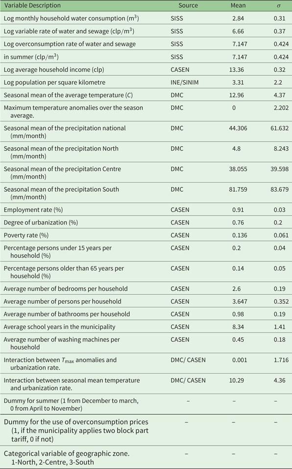
Variables use in modelling residential water demand in Chile

Notes: Seasonal means of precipitation are from averages across years and municipalities in the zone of interest. Urbanization rate: Percentage of households in an urban zone per municipality. Urban zone is defined as the set of households concentrated with population of more than 2000 people, or between 1001 and 2000 people with at least 50% of economically active population working on secondary or tertiary activity. For more information about demographic and socio demographic variables, review the web page of the CASEN survey: http://observatorio.ministeriodesarrollosocial.gob.cl/casen/casen_obj.php.

Although individual household consumption is unavailable, a panel of 42 municipalities with 13 years of monthly consumption levels, prices and weather variables was assembled for this study. Each water utility has its own rate structure. The basic rate structure of ‘real’ water prices is set by a process defined by law and re-structured every five years; real prices are maintained by adjusting nominal prices monthly to price indices, including the consumer price index.Footnote ⁴ When block pricing is present in a municipality, it is a two-block scheme applied only during the ‘peak period’ of summer (December to March). In this scheme the prices for the first block is termed the variable rate, and for the second block the ‘overconsumption’ rate. During the rest of the year, consumers face a uniform marginal rate. There are some municipalities, mainly in the south, which maintain a single tariff throughout the year. Although block-pricing structures are in place in some municipalities, and they are ostensibly intended to discourage consumption during the drier summer months, in reality the proportion of all households that surpass the consumption limit is small and concentrated in a few municipalities of our sample in one high-income geographic area.Footnote ⁵

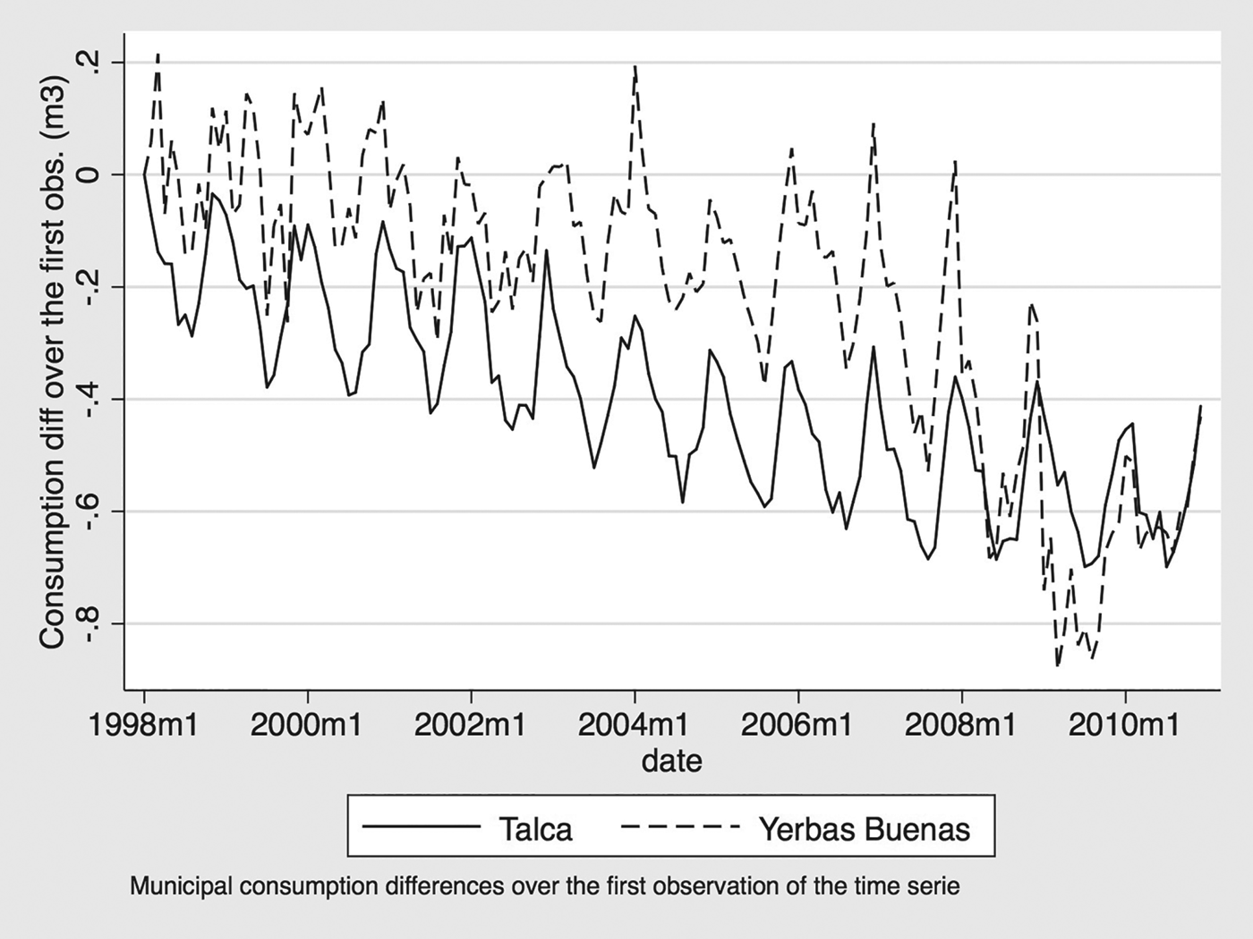
Although most studies of water demand are focused on the influence of prices and socio-demographic variables on consumption, there are studies that include weather-related variables such as temperature and precipitation as well as socioeconomic household characteristics (e.g., Nieswiadomy and Molina, Reference Nieswiadomy and Molina1989; Martinez-Espiñeira, Reference Martinez-Espiñeira2002; Neale, Reference Neale2005; Olmstead et al., Reference Olmstead, Hanemann and Stavins2007). These studies find strong correlations between water demand and temperature. There are some studies that show that residential consumption, especially outdoor use (gardens, swimming pool, lawn care, etc.) is dependent on climatic variables (Cohen, Reference Cohen1985; Akuoko-Asibey et al., Reference Akuoko-Asibey, Nkemdirim and Draper1993; Dandy et al., Reference Dandy, Nguyen and Davies1997). Worthington and Hoffman (Reference Worthington and Hoffman2008), in a survey of residential water demand modelling, conclude that there is no strong empirical evidence of scale economies with respect to household size. In addition, higher proportions of older and younger populations may cause an increase in water demand (Nauges and Thomas, Reference Nauges and Thomas2000; Martinez-Espiñeira, Reference Martinez-Espiñeira2003). With respect to the Chilean case, the country has a diverse range of climates, from the warm, arid north, to the temperate, dry-season centre, to the cooler, rainy south, resulting in a notable cross-sectional variation in the data. Interestingly, in our sample, less-urbanized municipalities have higher volatility in consumption than their more-urbanized counterparts. This is illustrated in figure 1 for two geographically-close municipalities in the same climate zone: Yerbas Buenas and Talca. The level of urbanization is correlated with greater regularity in the yearly cycle of water consumption, owing in part to a smaller fraction of drinking water consumption going to outdoors uses (gardens, irrigation, etc.), and making them less sensitive to climate variations.

Figure 1.

Consumption volatility of two municipalities, geographically close but very different in their urbanization indices.

Source: Authors calculations from data from SISS.

3. Data sources and the regression model

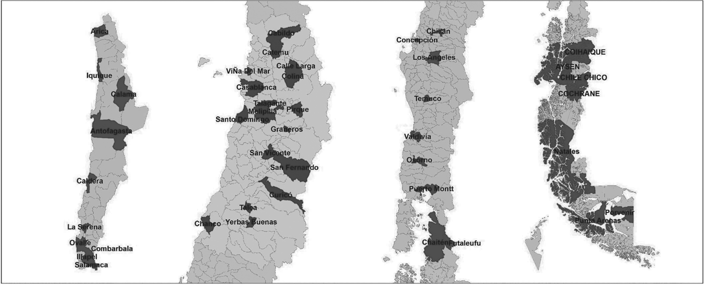
In this study we make use of a monthly panel from 1998 to 2010 of 42 municipalities scattered along the vertical axis that is Chile (figure 2). The panel is unbalanced due to the lack of a complete series of weather-related data for some municipalities. Consumption and water price information was collected from the state regulatory agency SISS (Superintendencia de Servicios Sanitarios). The periodic national household survey CASEN and the National Institute of Statistics (INE) are the sources of the socio-economic and demographic variables at the municipal level, such as average household size, income and so on (see table 1 for summary statistics of variables in our sample included in the modelling effort). The CASEN survey is completed every two or three years, and so five surveys are available for the 1998–2010 period. INE produces annual information on demographic characteristics at the municipal level. Simple linear interpolation was used to translate these data into monthly observations. The climate-related information comes from the databases of the Chilean Meteorological Administration (Dirección Meteorológica de Chile, DMC), which manages daily level data for at least one weather station within the 42 municipalities of the study; these data were aggregated to produce synthetic monthly observations. In interpreting the results below with respect to monthly average residential water use per household, the reader should keep in mind the possible additional error that might be generated by the interpolation of household characteristics.

Figure 2.

Chilean municipalities in the study sample.

The basic model of per-household water consumption (Q) to be estimated is in log-log form with idiosyncratic effects and a purely random shock:

(1)$$Q_{it}=\beta x_{it}+\nu _{i}+\varepsilon _{it},$$

where ν _i is the idiosyncratic effect for municipality i, and ε_it is the error that represents unexplained variations at each municipality i and month, t. After some appropriate tests, this error is modelled as a first-order autoregressive process.Footnote ⁶ Table 1 presents the explanatory variables in the estimated model, which has the following form:

(2)$$\eqalign{lnQ_{it} & = \alpha +\beta _{1}lnT_{it}^{v}+\beta _{2}lnT_{it}^{sc} {\ast} d_{it}^{p} {\ast} d_{it}^{sc} \cr & \quad +\gamma ^{\prime }Cl_{it}+\delta ^{\prime}Z_{it}+\theta ^{\prime }D_{it}+\nu _{i}+\varepsilon _{it},}$$

where $T_{it}^{v}$ represents the first-block variable tariff and $ T_{it}^{sc}$ the second-block overconsumption tariff, which is only appropriate during the summer months ($d_{it}^{p}=1$, 0 otherwise) and for the municipalities that make use of block pricing ($d_{it}^{sc}=1$, 0 otherwise). The vector of climate and weather variables is represented by Cl _it. Household and municipal characteristics (Z _it) include average household income and education, average household size, average number of bathrooms and washing machines per household, poverty rates, urbanity (the proportion of households living in urban areas within each municipality), and population per square kilometre. Dummies (D _it) for each month, the summer season and a municipality's seaside location are introduced to control for aspects of demand not captured by the other controls. The municipality idiosyncratic effects (ν _i) account for all excluded municipality characteristics relevant to water demand. After comparing and testing random- and fixed-effects, we opt for fixed effects.Footnote ⁷

Based on the raw daily data of temperature and precipitation, this study differentiates between changes across municipalities in seasonal averages (for the whole period), representing the ‘climate’ or the longer-term weather component, and within-season changes around these municipal-specific seasonal averages. Such within-season changes represent the ‘weather’ component or the short-term anomaly around the seasonal (climate) averages. This separation of effects also allows for a projection of the impact of a change in the longer-term component. This longer-term component is calculated as the seasonal aggregate of the climate variable for season s of the observed month (four seasons per year) and municipality i, (m = temperature or precipitation). The short-term anomaly of both climate measures is calculated as:

(3)$$M_{it}=m_{it}-\bar{m}_{it},$$

where m _it is the weather variable (temperature or precipitation) for municipality i and month t.

To be clear, the two long-run measures of each municipality's climate (mean temperature and precipitation) vary by season. That is, for any observation of, for example, mean temperature, there are four different values possible for each municipality, but these values will repeat year to year. The reader should note that these are not seasonal dummies. The seasonal temperature mean has an estimated coefficient associated with it which is the same regardless of whether the season is, for example, summer or winter.Footnote ⁸ Precipitation is measured straightforwardly as millimetres per month, and the average is calculated using all 13 years for each of the three-month seasons.Footnote ⁹ For the temperature seasonal aggregate, each municipality's average daily mean temperature across all years of the data is used. For the short-term weather variable, this study makes use of the monthly average daily maximum temperature anomalies. This variable of monthly average daily maximum temperatures was employed, because it varies over the year significantly more than the average minimum, which is quite stable, and the average daily mean. The short-term maximum temperature anomaly is defined as a deviation about the municipality-specific average for each season. The season average climate and short-term weather anomalies variables (for both temperature and precipitation) enter the above regression equation in the following way: $ \gamma ^{\prime }Cl_{it}=\gamma _{\bar {m}}\bar {m}_{is}+\gamma _{M}M_{it}$. Note that in the panel-data analysis, the introduction of municipality-specific effects does not eliminate the season-dependent climate variables. Alternative specifications of the variable representing short-term temperature fluctuations were tested: anomalies of each month's average daily mean around the long-run average daily mean for that month and for the season, and anomalies of each month's average minimum around its long-run average for that month and for the season. The econometric results for the main variables of interest (price, income, long-run average temperature, demographic, etc.) were robust to the use of these alternatives.Footnote ¹⁰

In addition, to account for possible non-linearity of effects of the climate and weather variables, we also test for the inclusion of quadratic terms (including a temperature-precipitation interaction). Non-linear effects would be of particular interest for projecting the possible influence on residential water demand of future climate change. As climate begins to move from its accustomed pattern, towards, say, higher average temperatures and less precipitation, households would alter their water use within the constraint given by former technologies and habits adapted to prior conditions. But, as expected temperatures and precipitation deviate farther from the former pattern, households would invest in what would become more appropriate technologies and develop new routines and habits of water consumption. For example, in the case of the central semi-arid zone of Chile, there would likely be households which would move from what is now the frequently observed handheld-hose watering of grass lawns toward drip-irrigation of arid-garden plants, a change which would tend to stabilize and insulate water demand from further temperature and precipitation changes. In short, the marginal effects of mean temperature increases and mean precipitation decreases could decline as climate change progresses.

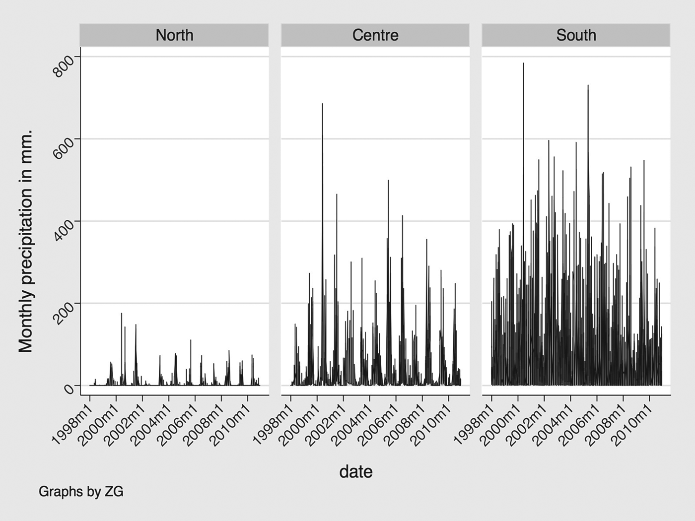
There is a notable pattern to the amount and frequency of precipitation across municipalities, from north to south, which can be grouped in the three macro-geographical zones usually defined by climatologist, as shown in figure 3. Precipitation patterns were incorporated into the model as an interaction between the seasonal average monthly precipitation and a dummy variable indicating the geographic area (Centre and South). Also, an interaction between temperature variables and urbanization rate was incorporated to test if consumption in more-urbanized municipalities is less sensitive to changes in temperature.

Figure 3.

Monthly total precipitation by Chilean geographic zone.

Source: Authors' calculations from meteorological data from Dirección Meteorológica de Chile (DMC).

4. Estimation results

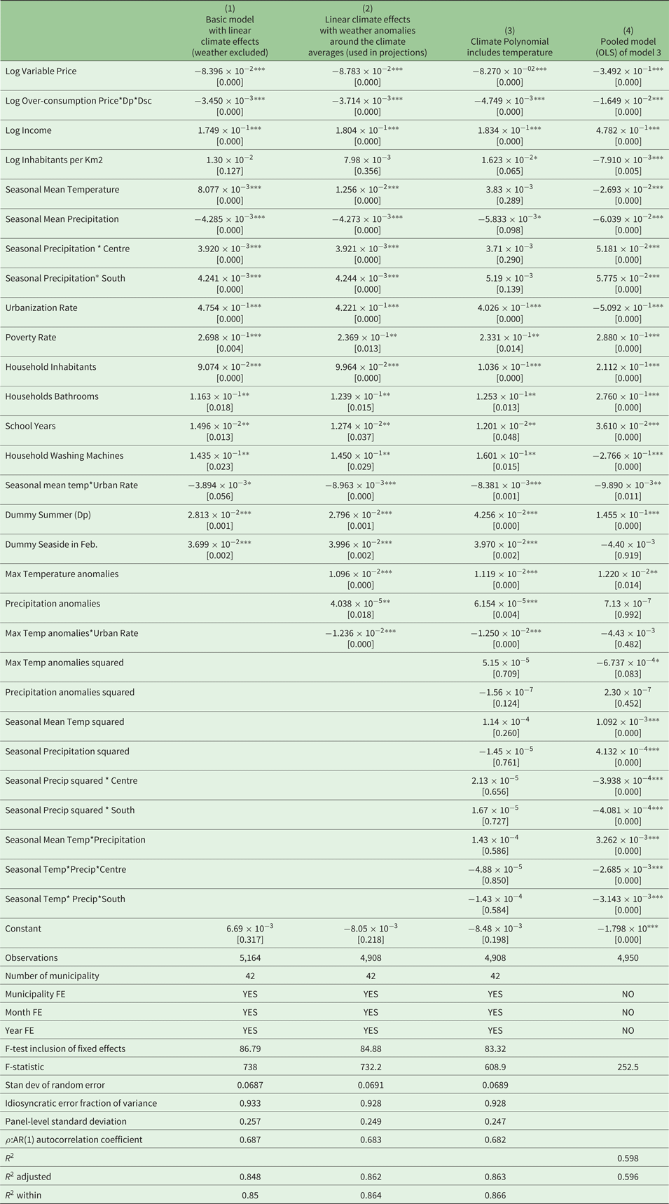
Table 2 shows the results of the fixed-effect estimation of three models and of a pooled model (without municipality and time effects) for comparison.Footnote ¹¹ The basic models (columns 1 and 2) contain the price, income and demographic variables, the climate and weather variables in linear form, and the monthly, year and seasonal dummies. Column 2 differs from column 1 only in that the weather variables are included (the anomalies around the long-run seasonal averages).Footnote ¹² Note that the estimated coefficients associated with the economic variables (prices and income) are robust in sign and order of magnitude with respect to the inclusion of additional variables in columns 2 and 3, although the absolute value of the over-consumption price increases somewhat when the quadratic terms of the climate and weather variables are included in the model of column 3. The results indicate an income elasticity of approximately 0.18 and a price elasticity of approximately −0.08. The values of these elasticity estimates are quite consistent with the evidence from the literature (Martinez-Espiñeira, Reference Martinez-Espiñeira2002; Arbués et al., Reference Arbués, Garcia-Valiñas and Martinez-Espiñeira2003; Martinez-Espiñeira and Nauges, Reference Martinez-Espiñeira and Nauges2004; Arbués and Villanúa, Reference Arbués and Villanúa2006). Nevertheless, it is worth noting that, in comparing these results to other estimated models not shown here, the introduction of the year fixed effects reduces the absolute value of the price elasticity, suggesting trends in water consumption not accounted for by the inclusion of socio-economic variables which have shown significant trends in the case of Chile during the period of study (income, density of inhabitants, and washing machines and bathrooms per household). Likely there are other factors contributing to a trend in reduced water use, perhaps associated with increased country-wide efficiency as real water prices have drifted upward. The coefficient on the ‘overconsumption’ – the second block – price is statistically significant but, practically speaking, very small, close to −0.004, in all models with municipal and time dummies. As noted previously, the overconsumption price is paid by only a small fraction of users, and so a small effect on average residential household water use is unsurprising. Nevertheless, the results do imply that there could be policy-induced reductions, although small, in water demand via either raising the overconsumption price or reducing the trigger level of consumption or a combination of both measures.

Table 2.

Estimation results

t statistics in parentheses, and * p<0.10, ** p<0.05, *** p<0.01.

We note that the introduction of the climate and weather-related variables in a linear manner (columns 1 and 2) captures the seasonality of demand. The coefficient associated with long-term temperature – the seasonal mean temperature – is approximately 0.013 in this simple linear model (and we note, although not reported here, that the coefficient remains at that value regardless of the inclusion of municipal, socio-economic variables). This value implies slightly more than a one per cent increase in per-household water consumption for a 1^° Celsius increase in the (long-term) seasonal average temperature. The coefficient associated with the monthly temperature variations around the seasonal average – maximum temperature anomalies – is approximately of the same order magnitude (0.011), which would imply that water demand reacts to short-term temperature increases in a similar manner as it does to longer-term temperature increases associated with climate changes.

The variation in average seasonal precipitation has a statistically significant impact in the north, but the practical effects of average precipitation changes appear very small in the centre and the south. In the north, an increase in one millimetre of precipitation leads to slightly less than a one-half percentage point decline in water consumption. For most municipalities in the far north, the range of the means of precipitation between the dry and wet seasons is usually less than one millimetre. There are, however, a few municipalities abutting the Andes where the change in precipitation from one season to another is large; in the municipality of Ovalle for example (see the first panel of figure 2), mean summer precipitation is less than one-half millimetre and the mean in winter is 16 millimetres, which would translate into an approximately 8 percentage-point decrease in per household water demand during the winter simply due to the precipitation cycle. There are two other northern municipalities where the practical impact on water demand of the swings in mean seasonal precipitation is pronounced, but for most communities across Chile the marginal impact of precipitation is small, if not – as in the centre and southern zones – effectively zero.

A more realistic specification, which would account for possible non-linear effects of the climate and weather variables (and possible interaction effects between temperature and precipitation), is given in column 3 in table 2. The reader will note that the estimated coefficients on the quadratic and interaction terms appear not to be statistically significantly different from zero using standard t-tests. Nonetheless, F-tests for the inclusion of the quadratic and interaction terms indicate rejection of the hypotheses that they added no additional information despite the large individual p-values. Although in some specifications without year effects (not shown here), results indicate that these quadratic terms have relatively small effects on goodness-of-fit measures, the more complete specification with non-linear terms leads to noteworthy differences in the projection results, as shown below.

With respect to household and municipal characteristics, the estimated coefficients are significant at the 5 per cent level (usually much less) in all models. The average number of persons per household has a positive effect on water consumption; a one-person increase translates into a 10 per cent increase in water consumption. A similar magnitude in the effect of an additional bathroom is found, though only significant at a 5 per cent significance level. At the margin, a decrease in the level of poverty would have a negative impact on water use (a decline of poverty of 5 percentage points would reduce water consumption by slightly more than 1 per cent). But note that this latter result is a ceteris paribus one, holding constant income levels, household inhabitants, average number of bathrooms and washing machines, etc.; it does not imply that one would observe the average poor household consuming more water than the average richer household, all other characteristics changing in correlation with income; poverty rates are likely correlated across municipalities and through time with the lower average efficiency of household water use by the poor. It should also be noted that the existence of a means-tested subsidy to poor households that reduced the tariff up to a certain limit (Gómez-Lobo and Contreras, Reference Gómez-Lobo and Contreras2003) may be inducing higher consumption.

Of particular note is the coefficient on the municipality urbanization level, which is positive and statistically significant, and notably large in a practical sense. The models presented here include interactions between the urbanization level and the two temperature variables. Using these estimates, one finds that an increase in urbanization from a rural municipality of 10 per cent urban households to an urban municipality of 90 per cent would lead to an expected increase in average consumption per household of approximately 24 per cent. The conclusion is that Chile's trend toward greater urbanization is driving higher water consumption – but, again, ceteris paribus: in real-world observations, other factors are working simultaneously to reduce per-household consumption over time. Interestingly, both coefficients on the interaction terms (between mean temperature and urbanization and between max temperature anomalies and urbanization) are negative and on the order of about one per cent per 1^°Celsius, in models of column 2 and 3. These results confirm the suspicion, arising from simple graphical inspections of the variability of water use, that water consumption in more-urbanized municipalities is indeed less sensitive to changes in temperature, holding all else constant.

The longer-run effect of greater urbanization in Chile is therefore toward increased and more stable water consumption patterns. What might be driving these results? The definition of urban versus rural in Chile (as applied by the official household surveys) is based on the number of people living in settlements (towns), with some adjustment for the degree of the working population engaged in agriculture. An urban designation is correlated with population density and, given the low population limit for switching between zones, a rural designation is highly correlated with proximity to agricultural activities. We are accounting for various other household attributes that might be correlated with urban residency, such as income levels, washing machines, number of bathrooms, etc. But we do not have data on potential non-potable water use in rural areas. Chilean rural zones are served by various canals and aquifer wells, due to the extensive infrastructure necessary for agriculture to capture water fed by snowmelt runoff. Lawns that would otherwise be irrigated by metered, potable water from a piped network in urban zones would be more likely irrigated by non-potable water from canals or pumps in rural areas. Although more speculative, there could also be more household utility gained by lawn upkeep in urban settings as compared to rural settings, which potentially could also be a source of this urbanization effect on water demand.

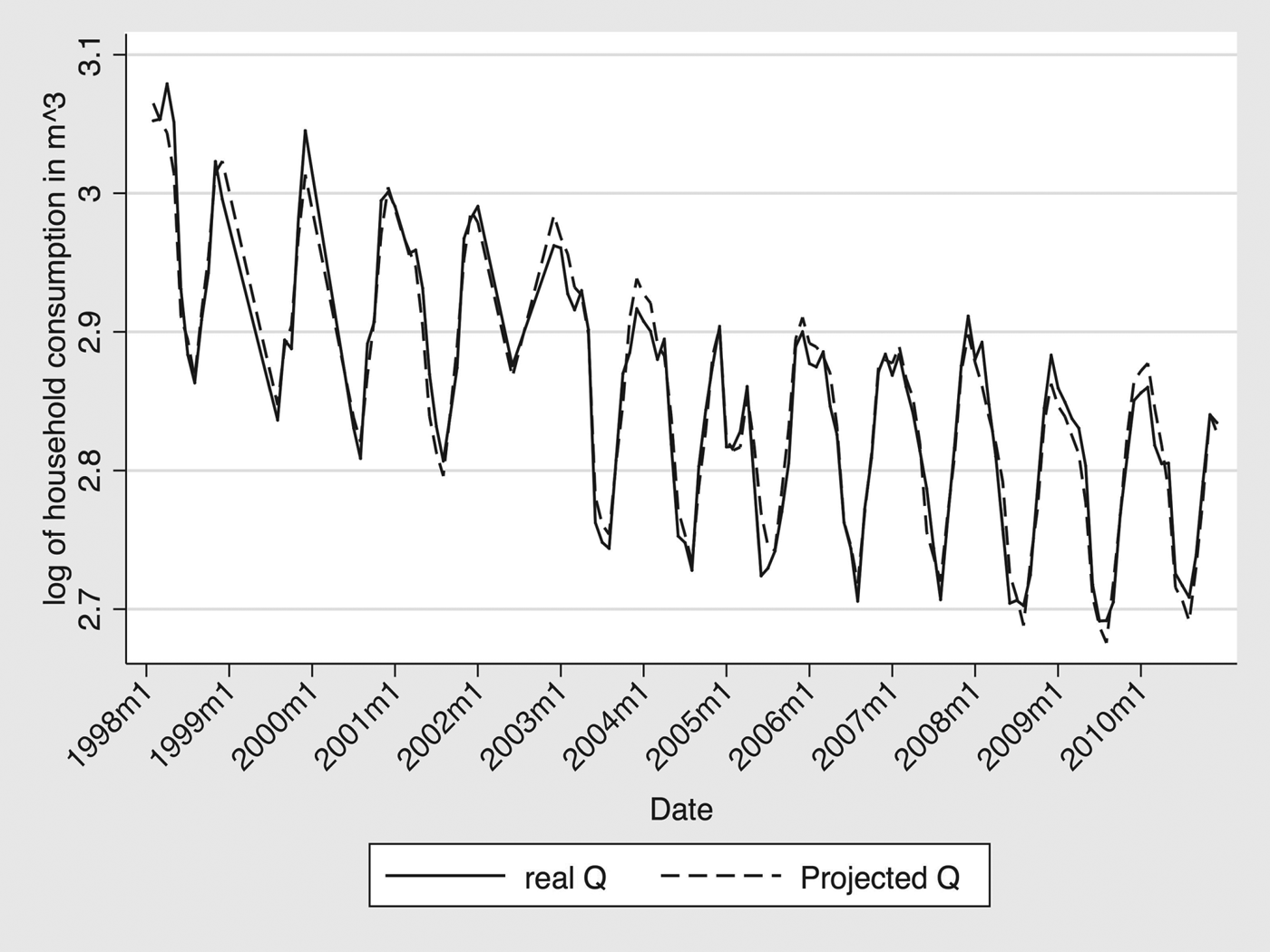
Finally, using the estimates from the models in column 3 of table 2, figure 4 presents observed and projected average monthly, per-household water consumption, averaged across the entire panel of municipalities for the period 1998–2010. We should note that the overall goodness of fit of the models in columns 1, 2 and 3 of table 2 in comparison with the pooled model in column 4 is enhanced by the introduction of monthly dummies, which not only affect the estimated coefficients on the variables of interest, but also help in fitting the regression line in the case of the crest and troughs in consumption, revealing that demand seasonality is not completely explained by our climate variables. The estimated models without and with non-linear effects of climate (columns 2 and 3) serve as the basis for projecting household water consumption under future climate scenarios, an application that is presented in the next section.

Figure 4.

Observed and projected average consumption 1998–2010.

Source: Authors' elaboration based on the results in table 2, column 3.

4.1 Application to the possible impacts of climate change on Chilean residential water use

As an application of the estimation results, an evaluation of the possible impacts of climate change on Chilean residential water use is presented (Neale (Reference Neale2005) is an example of the projection of the water demand under different climate-change scenarios). The projections are constructed on monthly averages based on the climate projections from the Providing Regional Climates for Impact Studies (PRECIS) model developed by the Hadley Centre of the United Kingdom Meteorological Office and adapted for use in Chile by the Department of Geophysics of the University of Chile (CONAMA, 2006).Footnote ¹³ The regional model PRECIS was used to derive information with greater spatial detail, in which the calculation domain covers only a part of the globe, and can be described with better resolution (25 km in this case) covering the entire continental territory of Chile. Such resolution is the maximum attainable with this model (CONAMA, 2006). These projections, which are at the level of 25 square kilometres, are for months between the years 2070 and 2100. The projections are broken into average water use by season for the three decades 2070–2080, 2080–2090 and 2090–2100. In addition to the baseline, there are two change scenarios, one more extreme than the other. The reference is the set of monthly averages during the period 1961–1990. The change scenarios simulate the supposed effects until 2100 of projected greenhouse gas emissions SRES A2 (severe) and SRES B2 (moderate).Footnote ¹⁴

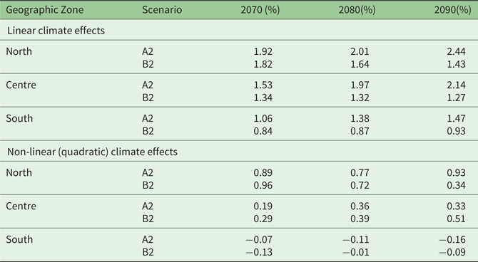
Average temperatures increase (2 to 4 degrees, under scenario A2), most notably during the summer, and precipitation rates tend to decline across Chile, with the exception of the arid north during the summer and the extreme south during the winter. Monthly simulations for temperature and precipitation from the PRECIS are averaged to obtain four seasonal averages by decade for both climate variables, introducing these average projections into the estimated models (columns 2 and 3 in table 2) and holding all other variables constant at their means of the three last years of observations (temperature and weather anomalies are set to zero). Table 3 presents the percentage changes in per-household consumption compared to the baseline. In the case of both linear and non-linear climate effects models, one notes that the greatest impact on per-household residential consumption is projected to occur in the arid north. The maximum average increase over the baseline, however, in the linear-climate-effect model is under 2.5 per cent, and in the non-linear case, under 1 per cent. Across all 42 municipalities, the national average increase in water use in both scenarios in the linear-effect is less than 1.5 per cent, and even smaller in the non-linear model. A few municipalities in the arid north have average increases of approximately 4–5 per cent in both cases. These greater consumption increases in these northern municipalities would be attributable both to increased average temperatures and, importantly, decreased precipitation.

Table 3.

Percentage change over the baseline by Geographic Zone

Source: Authors' calculations based on estimated coefficients in table 2 (columns 2 and 3) and PRECIS climate projections as discussed in text.

Water use projections based on the model specification with the non-linear climate effects show on average negligible changes (in fact, slightly negative value) in average consumption per household in the southern third of the country, where rainfall is currently relatively plentiful and temperatures lower compared to the arid and semi-arid zones to the north. These results underline the importance of the specification used for projecting future climate effects. Nevertheless, in both the linear and non-linear climate effect models these projected increases in water use due to climate are small compared to projections associated with likely increases in urbanization, decreases in poverty and other development-related changes. For example, an increase in the urbanization proportion of only 3 per cent (a small gain compared to recent history) would yield the same average increase as the climate projection in the stronger case of linear effects. A decline in poverty rates from 20 to 10 per cent (approximately the national decline during the 2000 s), ceteris paribus, would decrease average household consumption by 2.5. Using the point estimate of its coefficient in column 3 of table 2 (0.125), the addition of one extra bathroom on average – moving from the current sample average of slightly less than one bathroom to two per household (a reasonable projection for over the next generation) – would increase average water use by over six times the highest average projected increase linked to climate change (12.5 percent versus 2 per cent). Again, using the point estimate of its coefficient in column 3 of table 2 (0.160), moving from the current national average of 0.45 washing machines to 0.8, which would also be a reasonable increase in the coming generation, would be expected to increase average water use by over twice the highest projected increases in consumption associated with climate change over the next half-century (0.35*16.0 = 5.6 per cent versus 2 per cent).