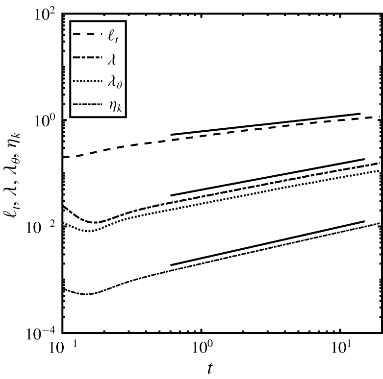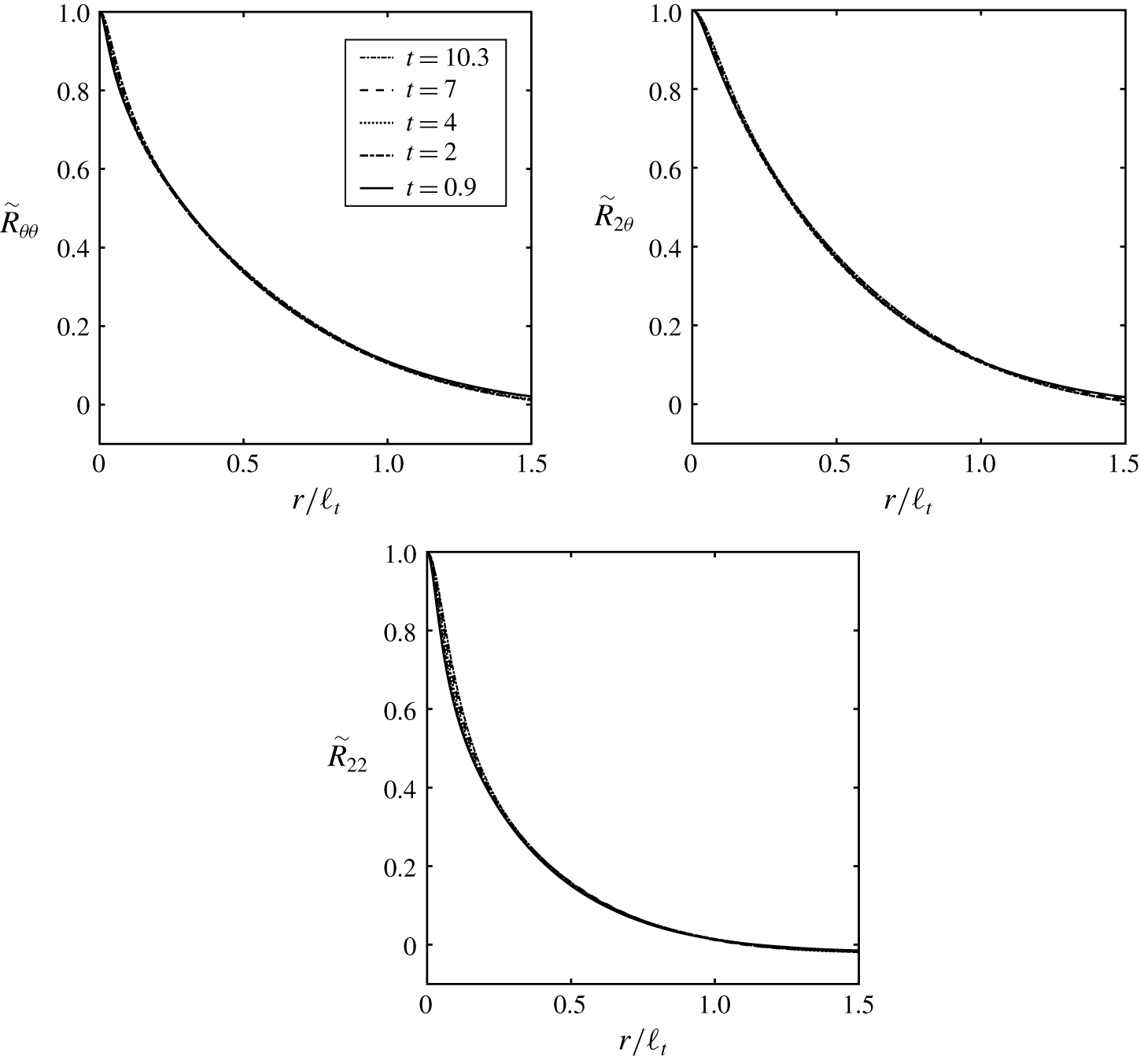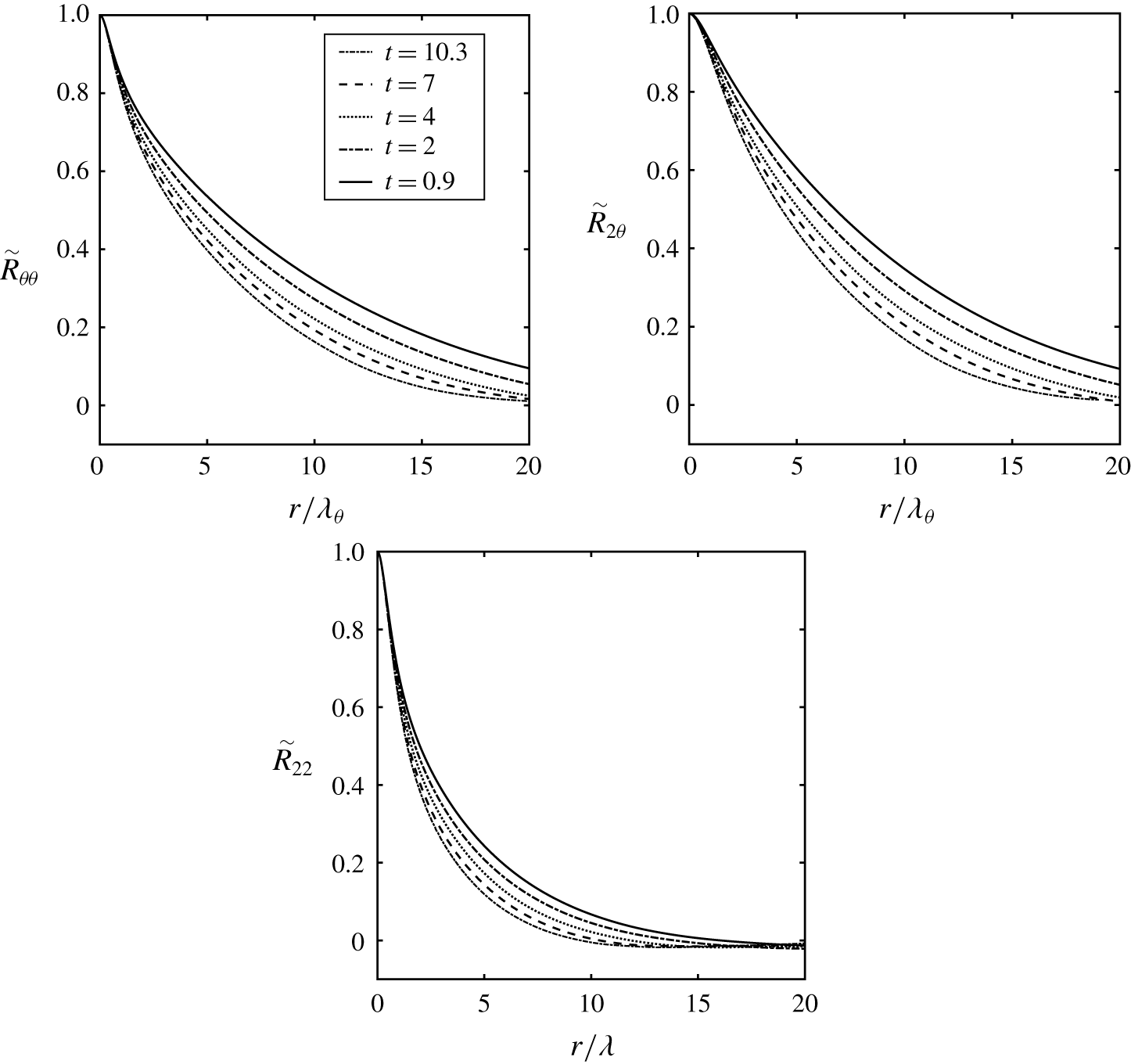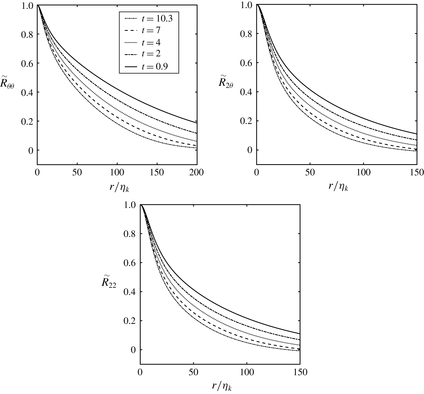


1 Introduction
The evolution of a passive scalar flow has been a subject of considerable interest in the research field of turbulence flows for the past 70 years. The primary reasons for the continuous interest in this topic are its important place in the development and verification of turbulence theories, in addition to its paramount beneficial effects in industry, such as the efficiency of combustion and discharged pollutants. Significant studies in the evolution of temperature fluctuations were put forward by Corrsin (Reference Corrsin1951a,Reference Corrsinb) in isotropic turbulence, in which the equations for the correlation functions and spectral functions were considered from which the scaling laws for the temperature fluctuations were derived therein. Thereafter, a significant amount of work has been devoted to establish the statistical characteristics of the passive scalar fields (especially the decay of temperature fluctuations) in turbulent flows (e.g. Warhaft & Lumley Reference Warhaft and Lumley1978; George Reference George1992b; Warhaft Reference Warhaft2000; Watanabe & Gotoh Reference Watanabe and Gotoh2004; Bahri et al. Reference Bahri, Arwatz, George, Mueller and Hultmark2015).
Although the evolution of a passive scalar field with a turbulent velocity field in the background has been traditionally studied in the literature by means of a wide range of theoretical, numerical and experimental methods, the fundamental basis to understand the statistical state of flow and to derive scaling laws has been self-similarity (or self-preservation) analysis. In the context of decaying homogeneous isotropic turbulence, von Kármán & Howarth (Reference von Kármán and Howarth1938) applied the first self-preservation hypothesis to the transport equation of the two-point (second-order) longitudinal velocity correlation function  $u$,
 $B_{LL}\equiv \overline{u(x+r)u(x)}$, i.e.
 $$\begin{eqnarray}\frac{\unicode[STIX]{x2202}B_{LL}}{\unicode[STIX]{x2202}t}=\frac{1}{r^{4}}\frac{\unicode[STIX]{x2202}}{\unicode[STIX]{x2202}r}\left[r^{4}\left(B_{LL,L}+2\unicode[STIX]{x1D708}\frac{\unicode[STIX]{x2202}B_{LL}}{\unicode[STIX]{x2202}r}\right)\right],\end{eqnarray}$$
where  $B_{LL,L}\equiv \overline{u^{2}(x+r)u(x)}$ is the third-order velocity correlation function,
 $r$ is the spatial separation in the longitudinal direction and
 $\unicode[STIX]{x1D708}$ is the kinematic viscosity. According to the hypothesis of von Kármán & Howarth (Reference von Kármán and Howarth1938), an a priori single length scale
 $l(t)$ and an a priori single velocity scale
 $u(t)$ are sufficient to derive the statistical moments of the fluctuating field. This hypothesis was applied to the two-point velocity correlation functions, i.e. considering
 $$\begin{eqnarray}B_{LL}(r,t)=\overline{u^{2}}(t)f(r/l(t))\end{eqnarray}$$
and
 $$\begin{eqnarray}B_{LL,L}(r,t)=\overline{u^{2}}(t)^{3/2}k(r/l(t)),\end{eqnarray}$$
where  $f$ and
 $k$ are the self-similar functions, and
 $\overline{u^{2}}(t)$ is the variance of the velocity fluctuations. In the limit of small
 $\unicode[STIX]{x1D708}$, a self-similar form of (1.1) may be generated, which in turn describes the decay of isotropic turbulence.
Similarly, Corrsin (Reference Corrsin1951a) applied the same approach as von Kármán & Howarth (Reference von Kármán and Howarth1938) to the isotropic temperature fluctuations in decaying isotropic turbulence, and he obtained
 $$\begin{eqnarray}\frac{\unicode[STIX]{x2202}B_{\unicode[STIX]{x1D703}\unicode[STIX]{x1D703}}}{\unicode[STIX]{x2202}t}=\frac{2}{r^{2}}\frac{\unicode[STIX]{x2202}}{\unicode[STIX]{x2202}r}\left[r^{2}\left(B_{L\unicode[STIX]{x1D703},\unicode[STIX]{x1D703}}+\unicode[STIX]{x1D6FC}\frac{\unicode[STIX]{x2202}B_{\unicode[STIX]{x1D703}\unicode[STIX]{x1D703}}}{\unicode[STIX]{x2202}r}\right)\right],\end{eqnarray}$$
where  $\unicode[STIX]{x1D6FC}$ is the thermal diffusivity, the correlation functions are
 $B_{\unicode[STIX]{x1D703}\unicode[STIX]{x1D703}}\equiv \overline{\unicode[STIX]{x1D703}(x+r)\unicode[STIX]{x1D703}(x)}$ and
 $B_{L\unicode[STIX]{x1D703},\unicode[STIX]{x1D703}}\equiv \overline{u(x+r)\unicode[STIX]{x1D703}(x+r)\unicode[STIX]{x1D703}(x)}$, and
 $\unicode[STIX]{x1D703}$ is the temperature fluctuation.
Thereafter, the analysis of self-preservation has become a common tool in turbulence to derive the scaling laws for both the velocity and scalar quantities. In a series of important works, George (Reference George, George and Arndt1989, Reference George1992a) re-examined the possibility of a self-preserving solution to the spectral form of the equation from a more general perspective valid for both finite and infinite Reynolds numbers. George (Reference George1992a) applied his equilibrium similarity analysis for the decay of homogeneous isotropic turbulence by considering the spectral energy equation
 $$\begin{eqnarray}\frac{\unicode[STIX]{x2202}E(k)}{\unicode[STIX]{x2202}t}=T(k)-2\unicode[STIX]{x1D708}k^{2}E(k),\end{eqnarray}$$
where  $E(k)$ is the three-dimensional kinetic energy spectrum and
 $T(k)$ is the nonlinear spectral transfer function. This equation is the Fourier-space equivalent of (1.1). George (Reference George1992a) showed that all terms in (1.5) evolve in exactly the same manner, where the mean turbulent kinetic energy,
 $\overline{q^{2}}=(3/2)\overline{u^{2}}$, and the Taylor microscale,
 $\unicode[STIX]{x1D706}$, are used as the appropriate scaling parameters for normalization. In addition, it was shown that
 $\overline{q^{2}}$ decays as a power law in time, and
 $\unicode[STIX]{x1D706}$ grows as the square root of time. The coefficient and decay rate in the power-law equation were shown to be dependent on the initial conditions.
In the case of passive scalars, George (Reference George1992b) applied his analysis to equivalent spectral equations governing the decay of temperature fluctuations in isotropic turbulence, and similarly obtained that the relevant scales for the self-similarity are the scalar Taylor microscale,  $\unicode[STIX]{x1D706}_{\unicode[STIX]{x1D703}}$, and the scalar variance,
 $\overline{\unicode[STIX]{x1D703}^{2}}$. Further, he showed that the consequence of his analysis is in good agreement with the temperature spectra measured by previous experiments, such as those of Warhaft & Lumley (Reference Warhaft and Lumley1978).
In a recent work, Bahri et al. (Reference Bahri, Arwatz, George, Mueller and Hultmark2015) derived the conditions for self-preserving solutions for the evolution of a passive scalar in grid turbulence with a constant mean temperature gradient using the same self-preservation perspective as George (Reference George1992a,Reference Georgeb) and investigated the results using the experimental data. Their similarity analysis predicts that the scaling functions are expected to be related to the temperature variance and a characteristic length scale such as  $\unicode[STIX]{x1D706}_{\unicode[STIX]{x1D703}}$. Gauding et al. (Reference Gauding, Goebbert, Hasse and Peters2015), Gauding, Danaila & Varea (Reference Gauding, Danaila and Varea2017) and Gauding et al. (Reference Gauding, Wang, Goebbert, Boded, Danaila and Vareaa2019) also studied the self-similarity of a passive scalar in decaying homogeneous isotropic turbulence by the method of line segments. They found that, by using the classical Kolmogorov length scale,
 $\unicode[STIX]{x1D702}_{k}$, although the similarity of the normalized scalar correlation function is very poor, the self-preservation of the normalized derivative correlation function is satisfactory using this length scale.
As discussed, despite the fact that the classical self-similarity to construct scaling parameters for the passive scalars has been known for a long time, there are still several open challenges. First and foremost, the classical self-similarity hypothesis can only be carried out when using an a priori set of similarity scales for all of the statistical moments in the transport equations. Therefore, it is one of the outstanding goals to obtain the similarity scales based on a more general analytical approach rather than in an ad hoc manner. In addition, the interaction between the velocity and passive scalar (temperature) fields becomes important in several cases, for example, when a constant mean temperature gradient is present. However, the lack of a unified approach that can predict the direct link between the scaling laws for the passive scalar and velocity moments is noted in the literature.
Therefore, it is the main aim of this paper to use a more general technique, which is known as Lie symmetry analysis, to formally derive the scaling laws and similarity variables for a passive scalar flow advected by a turbulent flow. The application of Lie symmetry theory in turbulence has been developed by Oberlack and co-workers in several papers (see e.g. Oberlack Reference Oberlack2001; Oberlack & Rosteck Reference Oberlack and Rosteck2010; Oberlack et al. Reference Oberlack, Waclawczyk, Rosteck and Avsarkisov2015; Sadeghi, Oberlack & Gauding Reference Sadeghi, Oberlack and Gauding2018, Reference Sadeghi, Oberlack and Gauding2020). Their recent developments have been to derive a variety of classical and new scaling laws in turbulence through applying Lie symmetry theory to the infinite series of two-point correlation (TPC) and multi-point correlation (MPC) equations.
In the present research, we employ the Lie symmetry method to both the instantaneous and the TPC equations of a passive scalar flow advected by a statistically homogeneous isotropic and incompressible turbulent velocity field. Most importantly, for the scalar field it is assumed that a mean temperature field exists, which has a constant gradient  $\unicode[STIX]{x1D6E4}$. Hence, only the velocity field is isotropic, while the scalar field is not. As a consequence of the current analytical work, we propose new scaling laws for both the passive scalar and velocity moments. The results of direct numerical simulations (DNS) conducted by Gauding et al. (Reference Gauding, Goebbert, Hasse and Peters2015, Reference Gauding, Danaila and Varea2017, Reference Gauding, Wang, Goebbert, Boded, Danaila and Vareaa2019) are used to compare the new scaling laws.
This paper is organized as follows. The next section provides the basic ideas of Lie symmetries and invariant solutions. One example is included to understand the basic ideas of symmetries. The governing equations for the passive scalar dynamics in decaying homogeneous isotropic turbulence and the symmetry analysis of them are given in § 3. In § 4, we present the symmetries and derive invariant solutions, respectively the scaling laws, of the governing equations. The DNS details and verification of the scaling laws are presented in § 5. Finally, the summary and conclusions are drawn in § 6.
2 Lie symmetries
2.1 The theory of Lie groups
In this subsection, the basic ideas of Lie symmetries including that of invariant solutions are summarized, which is usually referred to as self-similar solution in the fluid mechanics community, if any scaling symmetries are involved. In the turbulence community, these types of invariant solutions are usually denoted turbulent scaling laws; however, they are in most cases not solutions of equations derived from first principles (such as the classical scaling laws, which are formulated in an ad hoc manner as noted in § 1).
Sophus Lie was the first to introduce symmetry analysis of a system of differential equations based on continuous transformation groups in order to unify and extend various specialized methods for solving differential equations. In simple language, when applying a symmetry transformation to equations, their formal structures remain unchanged. The reader is referred to the detailed description of this method in several textbooks, such as Hydon (Reference Hydon2000a) and Bluman, Cheviakov & Anco (Reference Bluman, Cheviakov and Anco2010); here we only briefly explain its major concepts below.
Suppose the system of partial differential equations under investigation is given by
 $$\begin{eqnarray}\boldsymbol{F}(\boldsymbol{x},\boldsymbol{y},\boldsymbol{y}^{(1)},\boldsymbol{y}^{(2)},\ldots )=0,\end{eqnarray}$$
where  $\boldsymbol{x}$ represents independent variables,
 $\boldsymbol{y}$ represents dependent variables and
 $\boldsymbol{y}^{(n)}$ represents the set of
 $n$th-order derivatives of
 $\boldsymbol{y}$ with respect to
 $\boldsymbol{x}$ including mixed derivatives. A symmetry or symmetry transformation of (2.1) is defined by the following transformation:
 $$\begin{eqnarray}\boldsymbol{x}^{\ast }=\unicode[STIX]{x1D753}(\boldsymbol{x},\boldsymbol{y}),\quad \boldsymbol{y}^{\ast }=\unicode[STIX]{x1D74D}(\boldsymbol{x},\boldsymbol{y})\end{eqnarray}$$
if
 $$\begin{eqnarray}\boldsymbol{F}(\boldsymbol{x},\boldsymbol{y},\boldsymbol{y}^{(1)},\boldsymbol{y}^{(2)},\ldots )=0\quad \Longleftrightarrow \quad \boldsymbol{F}(\boldsymbol{x}^{\ast },\boldsymbol{y}^{\ast },\boldsymbol{y}^{\ast (1)},\boldsymbol{y}^{\ast (2)},\ldots )=0\end{eqnarray}$$
holds. Further, instantly we can identify that a symmetry (2.2) maps a solution of (2.1) to a new solution of (2.1).
The target of the symmetry analysis is to find all Lie symmetries
 $$\begin{eqnarray}\boldsymbol{x}^{\ast }=\unicode[STIX]{x1D753}(\boldsymbol{x},\boldsymbol{y};\unicode[STIX]{x1D700}),\quad \boldsymbol{y}^{\ast }=\unicode[STIX]{x1D74D}(\boldsymbol{x},\boldsymbol{y};\unicode[STIX]{x1D700}),\end{eqnarray}$$
where  $\unicode[STIX]{x1D700}$ is called the group parameter. Since
 $\unicode[STIX]{x1D700}$ may take any value in
 $\unicode[STIX]{x1D700}\in \mathbb{R}$, equation (2.4) is also called the continuous group. Furthermore, and without loss of generality, it is assumed that the unitary transformation corresponds to
 $\unicode[STIX]{x1D700}=0$, i.e.
 $$\begin{eqnarray}\boldsymbol{x}^{\ast }=\unicode[STIX]{x1D753}(\boldsymbol{x},\boldsymbol{y};\unicode[STIX]{x1D700}=0)=\boldsymbol{x},\quad \boldsymbol{y}^{\ast }=\unicode[STIX]{x1D74D}(\boldsymbol{x},\boldsymbol{y};\unicode[STIX]{x1D700}=0)=\boldsymbol{y}.\end{eqnarray}$$
For the analysis below and in the subsequent derivation of the turbulent scaling laws, it is almost imperative to introduce infinitesimal transformations by doing a Taylor series expansion of the transformation groups (2.4) about  $\unicode[STIX]{x1D700}=0$ to obtain
 $$\begin{eqnarray}\boldsymbol{x}^{\ast }=\unicode[STIX]{x1D753}(\boldsymbol{x},\boldsymbol{y};\unicode[STIX]{x1D700}=0)+\frac{\unicode[STIX]{x2202}\unicode[STIX]{x1D753}}{\unicode[STIX]{x2202}\unicode[STIX]{x1D700}}\bigg|_{\unicode[STIX]{x1D700}=0}\unicode[STIX]{x1D700}+O(\unicode[STIX]{x1D700}^{2}),\quad \boldsymbol{y}^{\ast }=\unicode[STIX]{x1D74D}(\boldsymbol{x},\boldsymbol{y};\unicode[STIX]{x1D700}=0)+\frac{\unicode[STIX]{x2202}\unicode[STIX]{x1D74D}}{\unicode[STIX]{x2202}\unicode[STIX]{x1D700}}\bigg|_{\unicode[STIX]{x1D700}=0}\unicode[STIX]{x1D700}+O(\unicode[STIX]{x1D700}^{2}).\end{eqnarray}$$
The first term on each of the right-hand sides can be replaced by (2.5) and terms of order  $O(\unicode[STIX]{x1D700})$ are formally replaced by
 $\unicode[STIX]{x1D743}$ and
 $\boldsymbol{\unicode[STIX]{x1D702}}$:
 $$\begin{eqnarray}\boldsymbol{x}^{\ast }=\boldsymbol{x}+\unicode[STIX]{x1D743}(\boldsymbol{x},\boldsymbol{y})\unicode[STIX]{x1D700}+O(\unicode[STIX]{x1D700}^{2}),\quad \boldsymbol{y}^{\ast }=\boldsymbol{y}+\boldsymbol{\unicode[STIX]{x1D702}}(\boldsymbol{x},\boldsymbol{y})\unicode[STIX]{x1D700}+O(\unicode[STIX]{x1D700}^{2}),\end{eqnarray}$$
where  $\unicode[STIX]{x1D743}$ and
 $\boldsymbol{\unicode[STIX]{x1D702}}$ are called infinitesimals. Note that this is a key feature of the Lie group method that the continuous transformation group (2.4) and its infinitesimal form (2.7) are fully equivalent. If the infinitesimal of a transformation is known, its global form can be determined by integrating the first-order system using Lie’s first theorem,
 $$\begin{eqnarray}\frac{\text{d}\boldsymbol{x}^{\ast }(\unicode[STIX]{x1D700})}{\text{d}\unicode[STIX]{x1D700}}=\unicode[STIX]{x1D743}(\boldsymbol{x}^{\ast }(\unicode[STIX]{x1D700}),\boldsymbol{y}^{\ast }(\unicode[STIX]{x1D700})),\quad \frac{\text{d}\boldsymbol{y}^{\ast }(\unicode[STIX]{x1D700})}{\text{d}\unicode[STIX]{x1D700}}=\boldsymbol{\unicode[STIX]{x1D702}}(\boldsymbol{x}^{\ast }(\unicode[STIX]{x1D700}),\boldsymbol{y}^{\ast }(\unicode[STIX]{x1D700}))\end{eqnarray}$$
with initial conditions
 $$\begin{eqnarray}\boldsymbol{x}^{\ast }(\unicode[STIX]{x1D700})=\boldsymbol{x}\quad \text{and}\quad \boldsymbol{y}^{\ast }(\unicode[STIX]{x1D700})=\boldsymbol{y}\quad \text{at }\unicode[STIX]{x1D700}=0.\end{eqnarray}$$
Further, it should be noted that the actual calculation of all admitted symmetries of a given differential equation can essentially only be derived using the infinitesimal form of the symmetries (see e.g. Bluman et al. Reference Bluman, Cheviakov and Anco2010).
One important consequence of the symmetry analysis is that, when the symmetries of a differential equation are obtained, it is possible to derive invariant solutions from it. As noted earlier, this is particularly important in fluid mechanics and turbulence studies, as we can construct invariant solutions from first principles through symmetry. It should be noted that the current definition of a group invariant solution has been previously provided in Sadeghi et al. (Reference Sadeghi, Oberlack and Gauding2018, Reference Sadeghi, Oberlack and Gauding2020) and here it is only briefly reviewed due to its necessity for the present work. Similar to Sadeghi et al. (Reference Sadeghi, Oberlack and Gauding2018, Reference Sadeghi, Oberlack and Gauding2020) we define  $\boldsymbol{y}=\unicode[STIX]{x1D73B}(\boldsymbol{x})$ as an invariant solution of a differential equation if:
(i)
 $\boldsymbol{y}-\unicode[STIX]{x1D73B}(\boldsymbol{x})$ is an invariant function with respect to the operator X, (2.10)where X is given by$$\begin{eqnarray}\text{X}[\boldsymbol{y}-\unicode[STIX]{x1D73B}(\boldsymbol{x})]=0\quad \text{with}\quad \boldsymbol{y}=\unicode[STIX]{x1D73B}(\boldsymbol{x})\end{eqnarray}$$(2.11)$$\begin{eqnarray}\text{X}=\unicode[STIX]{x1D709}_{i}\frac{\unicode[STIX]{x2202}}{\unicode[STIX]{x2202}x_{i}}+\unicode[STIX]{x1D702}_{j}\frac{\unicode[STIX]{x2202}}{\unicode[STIX]{x2202}y_{j}},\end{eqnarray}$$
(ii)
$\boldsymbol{y}=\unicode[STIX]{x1D73B}(\boldsymbol{x})$ is a solution of a differential equation ($\boldsymbol{F}=0$).


Differentiating equation (2.10), we obtain the hyperbolic system
 $$\begin{eqnarray}\unicode[STIX]{x1D709}_{k}(\boldsymbol{x},\unicode[STIX]{x1D73B})\frac{\unicode[STIX]{x2202}\unicode[STIX]{x1D701}_{l}}{\unicode[STIX]{x2202}x_{k}}=\unicode[STIX]{x1D702}_{l}(\boldsymbol{x},\unicode[STIX]{x1D73B}),\end{eqnarray}$$
to be solved by the method of characteristics, which finally ends up with the characteristic condition
 $$\begin{eqnarray}\displaystyle \frac{\text{d}x_{1}}{\unicode[STIX]{x1D709}_{1}(\boldsymbol{x},\boldsymbol{y})}=\frac{\text{d}x_{2}}{\unicode[STIX]{x1D709}_{2}(\boldsymbol{x},\boldsymbol{y})}=\cdots =\frac{\text{d}x_{m}}{\unicode[STIX]{x1D709}_{m}(\boldsymbol{x},\boldsymbol{y})}=\frac{\text{d}y_{1}}{\unicode[STIX]{x1D702}_{1}(\boldsymbol{x},\boldsymbol{y})}=\frac{\text{d}y_{2}}{\unicode[STIX]{x1D702}_{2}(\boldsymbol{x},\boldsymbol{y})}=\cdots =\frac{\text{d}y_{m}}{\unicode[STIX]{x1D702}_{n}(\boldsymbol{x},\boldsymbol{y})}, & & \displaystyle\end{eqnarray}$$
where  $\unicode[STIX]{x1D73B}$ has been replaced by
 $\boldsymbol{y}$. The latter is usually referred to as an invariant surface condition.
2.2 Basic example: one-dimensional heat equation
The basic ideas of the symmetries and invariant solutions may be best illuminated by utilizing the one-dimensional heat equation:
 $$\begin{eqnarray}\frac{\unicode[STIX]{x2202}T}{\unicode[STIX]{x2202}t}-\frac{\unicode[STIX]{x2202}^{2}T}{\unicode[STIX]{x2202}x^{2}}=0.\end{eqnarray}$$
This equation admits six symmetry groups, two of which are scaling symmetries and are given by
 $$\begin{eqnarray}t^{\ast }=\exp (2\unicode[STIX]{x1D6FC})t,\quad x^{\ast }=\exp (\unicode[STIX]{x1D6FC})x,\quad T^{\ast }=T,\end{eqnarray}$$
and
 $$\begin{eqnarray}t^{\ast }=t,\quad x^{\ast }=x,\quad T^{\ast }=\exp (\unicode[STIX]{x1D6FD})T.\end{eqnarray}$$
If we combine (2.15) and (2.16), we can derive
 $$\begin{eqnarray}t^{\ast }=\exp (2\unicode[STIX]{x1D6FC})t,\quad x^{\ast }=\exp (\unicode[STIX]{x1D6FC})x,\quad T^{\ast }=\exp (\unicode[STIX]{x1D6FD})T,\end{eqnarray}$$
from which it follows that, if an equation admits more than one symmetry group, also any arbitrary combination of these symmetries is a symmetry, in fact a multi-parameter symmetry group. It is evident that conditions (2.3) are fulfilled since the implementation of (2.17) into (2.14) leaves the equation invariant if written in the new variables denoted by  $^{\ast }$, i.e.
 $(\unicode[STIX]{x2202}T^{\ast }/\unicode[STIX]{x2202}t^{\ast })-(\unicode[STIX]{x2202}^{2}T^{\ast }/\unicode[STIX]{x2202}x^{\ast 2})=0$ is equivalent to (2.14) since the factors
 $\exp (\unicode[STIX]{x1D6FC})$ and
 $\exp (\unicode[STIX]{x1D6FD})$ cancel out. Using (2.6) and (2.7), the symmetries in (2.15) and (2.16) can be presented in terms of its infinitesimals:
 $$\begin{eqnarray}\unicode[STIX]{x1D709}_{t}=2\unicode[STIX]{x1D6FC}t,\quad \unicode[STIX]{x1D709}_{x}=\unicode[STIX]{x1D6FC}x,\quad \unicode[STIX]{x1D702}_{T}=\unicode[STIX]{x1D6FD}T.\end{eqnarray}$$
The corresponding characteristic equations for the invariant solutions, i.e. (2.13) of the symmetries in (2.18a-c), read as
 $$\begin{eqnarray}\frac{\text{d}t}{2\unicode[STIX]{x1D6FC}t}=\frac{\text{d}x}{\unicode[STIX]{x1D6FC}x}=\frac{\text{d}T}{\unicode[STIX]{x1D6FD}t},\end{eqnarray}$$
from which we arrive at the following invariants:
 $$\begin{eqnarray}\tilde{x}=\frac{x}{\sqrt{t}},\quad \tilde{T}=\frac{T}{t^{\unicode[STIX]{x1D6FD}/2\unicode[STIX]{x1D6FC}}}.\end{eqnarray}$$
The invariants (2.20) correspond to the known invariant solutions of the heat equation (2.14). Introducing  $\tilde{T}$ in (2.20) as a new dependent variable, i.e.
 $T=t^{\unicode[STIX]{x1D6FD}/2\unicode[STIX]{x1D6FC}}\tilde{T}(\tilde{x})$, and
 $\tilde{x}$ as the similarity coordinate, and employing these in (2.14) leads to the ordinary differential equation
 $$\begin{eqnarray}\frac{\text{d}^{2}\tilde{T}}{\text{d}\tilde{x}^{2}}+\frac{1}{2}\tilde{x}\frac{\text{d}\tilde{T}}{\text{d}\tilde{x}}-\frac{\unicode[STIX]{x1D6FD}}{2\unicode[STIX]{x1D6FC}}\tilde{T}=0,\end{eqnarray}$$
which has solutions in special functions. Finally, the above example can be used to simply explain the notion of symmetry breaking, as this notion is very important and will be used later to construct scaling laws. As we can see, the solution (2.20) of the heat equation contains a number of undetermined parameters ( $\unicode[STIX]{x1D6FC}$ and
 $\unicode[STIX]{x1D6FD}$), which can be used to adapt to different boundary and initial conditions. In order to do so, we need to set one or more parameters to specific values. This is referred to as symmetry breaking, since some symmetries are violated by boundary conditions. For the above example of the heat equation, if we assume the boundary conditions
 $T(x=0,t)=T_{0}$, it is apparent from (2.20) that this leads to the symmetry breaking
 $\unicode[STIX]{x1D6FD}=0$.
2.3 Symmetries of Navier–Stokes, Euler and energy equations
In the following, we will provide more specific examples for the principal equations, which are also the basis for the theory that follows. Here, we consider the Navier–Stokes and thermal energy equations for an incompressible fluid. In a Cartesian coordinate system, under the restriction of constant density and viscosity, we have the momentum and continuity equations
 $$\begin{eqnarray}\frac{\unicode[STIX]{x2202}U_{i}}{\unicode[STIX]{x2202}t}+U_{k}\frac{\unicode[STIX]{x2202}U_{i}}{\unicode[STIX]{x2202}x_{k}}=-\frac{\unicode[STIX]{x2202}P}{\unicode[STIX]{x2202}x_{i}}+\unicode[STIX]{x1D708}\frac{\unicode[STIX]{x2202}^{2}U_{i}}{\unicode[STIX]{x2202}x_{k}\unicode[STIX]{x2202}x_{k}},\quad \frac{\unicode[STIX]{x2202}U_{k}}{\unicode[STIX]{x2202}x_{k}}=0,\end{eqnarray}$$
where  $t\in \mathbb{R}^{+}$,
 $\boldsymbol{x}\in \mathbb{R}^{3}$,
 $\boldsymbol{U}=\boldsymbol{U}(\boldsymbol{x},t)$ and
 $P=P(\boldsymbol{x},t)$, respectively, represent time, position vector, instantaneous velocity vector and pressure, while pressure has been normalized by a constant density. In the limit of zero viscosity
 $\unicode[STIX]{x1D708}=0$, i.e. the Euler equations, the system (2.22) admits a 10-parameter symmetry group, including the following three symmetry transformation groups, here given in global form (see e.g. Oberlack Reference Oberlack2001; Oberlack & Rosteck Reference Oberlack and Rosteck2010):
 $$\begin{eqnarray}\displaystyle T_{1}:\quad t^{\ast }=t,\quad \boldsymbol{x}^{\ast }=\exp (a_{1})\boldsymbol{x},\quad \boldsymbol{U}^{\ast }=\exp (a_{1})\boldsymbol{U},\quad P^{\ast }=\exp (2a_{1})P,\end{eqnarray}$$
 $$\begin{eqnarray}\displaystyle T_{2}:\quad t^{\ast }=\exp (a_{2})t,\quad \boldsymbol{x}^{\ast }=\boldsymbol{x},\quad \boldsymbol{U}^{\ast }=\exp (-a_{2})\boldsymbol{U},\quad P^{\ast }=\exp (-2a_{2})P,\end{eqnarray}$$
 $$\begin{eqnarray}\displaystyle T_{3}:\quad t^{\ast }=t+a_{3},\quad \boldsymbol{x}^{\ast }=\boldsymbol{x},\quad \boldsymbol{U}^{\ast }=\boldsymbol{U},\quad P^{\ast }=P,\end{eqnarray}$$
where  $a_{1}$,
 $a_{2}$ and
 $a_{3}$ are independent group parameters. The physical meaning of
 $T_{3}$ is a time translation, and
 $T_{1}$ and
 $T_{2}$ are, respectively, the scaling symmetries in space and time.
Invoking a formal transfer from Euler to Navier–Stokes equations, symmetry properties change, i.e. the two scaling symmetries  $T_{1}$ and
 $T_{2}$ recombine into a single group of the form
 $$\begin{eqnarray}T_{NS}:\quad t^{\ast }=\exp (2a_{1})t,\quad \boldsymbol{x}^{\ast }=\exp (a_{1})\boldsymbol{x},\quad \boldsymbol{U}^{\ast }=\exp (-a_{1})\boldsymbol{U},\quad P^{\ast }=\exp (-2a_{1})P,\end{eqnarray}$$
with  $a_{2}=2a_{1}$, and hence viscosity may be considered symmetry breaking. Further, the Navier–Stokes and Euler equations admit the Galilean group, which we will not repeat here, as we focus on those symmetries that will be important in the context of the current work.
As noted in the previous subsection, one important characteristic of the symmetry transformations is that they can be combined into a multi-parameter group, which also represents a symmetry. For example, the two scaling symmetries of  $T_{1}$ and
 $T_{2}$, (2.23a-d) and (2.24a-d), can be combined to form a two-parameter symmetry group,
 $$\begin{eqnarray}T_{1\circ 2}:\quad t^{\ast }=\exp (a_{2})t,\quad \boldsymbol{x}^{\ast }=\exp (a_{1})\boldsymbol{x},\quad \boldsymbol{U}^{\ast }=\exp (a_{1}-a_{2})\boldsymbol{U},\quad P^{\ast }=\exp [2(a_{1}-a_{2})]P,\end{eqnarray}$$
which, by inserting (2.27a-d) into (2.22) with  $\unicode[STIX]{x1D708}=0$, clearly satisfies (2.3).
Now, we consider the transport equation for the passive scalar  $\unicode[STIX]{x1D6E9}$, namely the thermal energy equation for a fluid medium,
 $$\begin{eqnarray}\frac{\unicode[STIX]{x2202}\unicode[STIX]{x1D6E9}}{\unicode[STIX]{x2202}t}+U_{k}\frac{\unicode[STIX]{x2202}\unicode[STIX]{x1D6E9}}{\unicode[STIX]{x2202}x_{k}}=\unicode[STIX]{x1D6FC}\frac{\unicode[STIX]{x2202}^{2}\unicode[STIX]{x1D6E9}}{\unicode[STIX]{x2202}x_{k}\unicode[STIX]{x2202}x_{k}},\end{eqnarray}$$
which admits the following symmetries:
 $$\begin{eqnarray}\displaystyle T_{\unicode[STIX]{x1D703}1}:\quad t^{\ast }=t,\quad \boldsymbol{x}^{\ast }=\boldsymbol{x},\quad \boldsymbol{U}^{\ast }=\boldsymbol{U},\quad \unicode[STIX]{x1D6E9}^{\ast }=\exp (a_{\unicode[STIX]{x1D703}})\unicode[STIX]{x1D6E9},\end{eqnarray}$$
 $$\begin{eqnarray}\displaystyle T_{\unicode[STIX]{x1D703}3}:\quad t^{\ast }=t+a_{3},\quad \boldsymbol{x}^{\ast }=\boldsymbol{x},\quad \boldsymbol{U}^{\ast }=\boldsymbol{U},\quad \unicode[STIX]{x1D6E9}^{\ast }=\unicode[STIX]{x1D6E9},\end{eqnarray}$$
where  $a_{\unicode[STIX]{x1D703}}$ represents the scaling symmetry of
 $\unicode[STIX]{x1D6E9}$, while
 $a_{3}$ is again the translation symmetry in time.
Besides the symmetries discussed above, the systems (2.22) and (2.28) have further symmetries, namely, translation in space, Galilean invariance and rotational symmetry. For the present case of homogeneous isotropic turbulence, the momentum equation (2.22) shows that translation in space and Galilean invariance are irrelevant, because these symmetries are already fulfilled a priori by the statistical homogeneity. The same is true for rotational symmetry, which, also in the statistical sense, was used by the implication of isotropy. The symmetries mentioned above were explicitly used, for example, in the derivation of the von Kármán–Howarth equation, so that this equation is invariant related to the latter symmetries. With the temperature equation (2.28) the situation is different due to the imposition of the mean temperature gradient. Thereby both the translations and Galilean invariance are broken in the direction of  $x_{2}$. Translations and Galilean invariance persist in the remaining directions
 $x_{1}$ and
 $x_{3}$. Of the three rotation groups, only the one in the
 $x_{1}$–
 $x_{3}$ plane remains, as can be proved by inserting it in (2.28).
For the turbulence analysis to follow, the Navier–Stokes and energy equations are considered as the essential basis, which in turn will be employed to derive the two-point (or multi-point) equations describing the moment statistics of fluid turbulence.
It is important to note that all of these symmetries of the Navier–Stokes equation transfer to the equations of the multi-point formulation (see e.g. Oberlack & Rosteck Reference Oberlack and Rosteck2011). In addition to the symmetries stemming from the Navier–Stokes and the energy equations, an additional scaling group of all dependent variables is admitted, which was first discovered in Oberlack & Rosteck (Reference Oberlack and Rosteck2010), and later in Waclawczyk et al. (Reference Waclawczyk, Staffolani, Oberlack, Rosteck, Wilczek and Friedrich2014) it was shown that this symmetry is a measure of intermittency.
3 The basic governing equations
In the present study, we consider a passive scalar  $\unicode[STIX]{x1D6E9}$ advected by a statistically homogeneous isotropic and incompressible turbulent velocity field
 $\boldsymbol{U}$. Additionally, a uniform mean gradient
 $\unicode[STIX]{x1D6E4}$ is imposed on the scalar field in the
 $x_{2}$ direction. Following the Reynolds decomposition approach, the instantaneous scalar and velocity fields can be decomposed into their mean and their fluctuation values, e.g.
 $$\begin{eqnarray}\unicode[STIX]{x1D6E9}=\overline{\unicode[STIX]{x1D6E9}}+\unicode[STIX]{x1D703},\quad U_{k}=\overline{U}_{k}+u_{k},\end{eqnarray}$$
where  $\unicode[STIX]{x1D703}$ and
 $u_{k}$ are, respectively, the fluctuating parts of the scalar and velocity fields, while
 $\overline{\unicode[STIX]{x1D6E9}}$ is the mean scalar and
 $\overline{U}_{k}$ is the mean velocity. For the present case, they read
 $$\begin{eqnarray}\overline{\unicode[STIX]{x1D6E9}}=\unicode[STIX]{x1D6E4}x_{2}\end{eqnarray}$$
and
 $$\begin{eqnarray}\overline{U}_{k}=0.\end{eqnarray}$$
Furthermore, the scalar fluctuations  $\unicode[STIX]{x1D703}$ are assumed to be statistically homogeneous and together with (3.1) and (3.2), equation (2.28) changes to
 $$\begin{eqnarray}\frac{\unicode[STIX]{x2202}\unicode[STIX]{x1D703}}{\unicode[STIX]{x2202}t}+u_{k}\frac{\unicode[STIX]{x2202}\unicode[STIX]{x1D703}}{\unicode[STIX]{x2202}x_{k}}+u_{2}\unicode[STIX]{x1D6E4}=\unicode[STIX]{x1D6FC}\frac{\unicode[STIX]{x2202}^{2}\unicode[STIX]{x1D703}}{\unicode[STIX]{x2202}x_{k}\unicode[STIX]{x2202}x_{k}},\end{eqnarray}$$
whereas the equation for the velocity fluctuation reduces to
 $$\begin{eqnarray}\frac{\unicode[STIX]{x2202}u_{i}}{\unicode[STIX]{x2202}t}+u_{k}\frac{\unicode[STIX]{x2202}u_{i}}{\unicode[STIX]{x2202}x_{k}}=-\frac{\unicode[STIX]{x2202}p}{\unicode[STIX]{x2202}x_{i}}+\unicode[STIX]{x1D708}\frac{\unicode[STIX]{x2202}^{2}u_{i}}{\unicode[STIX]{x2202}x_{k}\unicode[STIX]{x2202}x_{k}},\end{eqnarray}$$
where  $p$ is the pressure fluctuation normalized by the density.
The base equations for the current analysis are the equations for the TPC of the fluctuating quantities. The concept of TPC is a parameter of considerable importance in the study of turbulence in fluid flows for a number of main reasons. First, in contrast to one-point statistics, they deliver additional information on the turbulence statistics, such as length scale. Second, in every higher moment equation, only one additional unclosed tensor appears, which is also rather different from one-point equations. Third, any one-point statistic can be derived from the two-point statistics.
Starting with (2.22) and (2.28), the following equations for the TPC of the fluctuating velocity and scalar can be derived (see e.g. Hinze Reference Hinze1959a):
 $$\begin{eqnarray}\displaystyle \hspace{-12.0pt} & & \displaystyle \frac{\text{D}R_{\unicode[STIX]{x1D703}\unicode[STIX]{x1D703}}}{\text{D}t}+R_{k\unicode[STIX]{x1D703}}\frac{\unicode[STIX]{x2202}\overline{\unicode[STIX]{x1D6E9}}(\boldsymbol{x},t)}{\unicode[STIX]{x2202}x_{k}}+R_{\unicode[STIX]{x1D703}k}\frac{\unicode[STIX]{x2202}\overline{\unicode[STIX]{x1D6E9}}(\boldsymbol{x},t)}{\unicode[STIX]{x2202}x_{k}}\bigg|_{\boldsymbol{x}+\boldsymbol{r}}+\left[\overline{U}_{k}(\boldsymbol{x}+\boldsymbol{r},t)-\overline{U}_{k}(\boldsymbol{x},t)\right]\frac{\unicode[STIX]{x2202}R_{\unicode[STIX]{x1D703}\unicode[STIX]{x1D703}}}{\unicode[STIX]{x2202}r_{k}}\nonumber\\ \displaystyle \hspace{-12.0pt} & & \displaystyle \quad +\,\frac{\unicode[STIX]{x2202}R_{(\unicode[STIX]{x1D703}k)\unicode[STIX]{x1D703}}}{\unicode[STIX]{x2202}x_{k}}-\frac{\unicode[STIX]{x2202}R_{(\unicode[STIX]{x1D703}k)\unicode[STIX]{x1D703}}}{\unicode[STIX]{x2202}r_{k}}+\frac{\unicode[STIX]{x2202}R_{\unicode[STIX]{x1D703}(\unicode[STIX]{x1D703}k)}}{\unicode[STIX]{x2202}r_{k}}-\unicode[STIX]{x1D6FC}\left[\frac{\unicode[STIX]{x2202}^{2}R_{\unicode[STIX]{x1D703}\unicode[STIX]{x1D703}}}{\unicode[STIX]{x2202}x_{k}^{2}}-2\frac{\unicode[STIX]{x2202}^{2}R_{\unicode[STIX]{x1D703}\unicode[STIX]{x1D703}}}{\unicode[STIX]{x2202}x_{k}\unicode[STIX]{x2202}r_{k}}+2\frac{\unicode[STIX]{x2202}^{2}R_{\unicode[STIX]{x1D703}\unicode[STIX]{x1D703}}}{\unicode[STIX]{x2202}r_{k}\unicode[STIX]{x2202}r_{k}}\right]=0,\end{eqnarray}$$
 $$\begin{eqnarray}\displaystyle \hspace{-12.0pt} & & \displaystyle \frac{\text{D}R_{i\unicode[STIX]{x1D703}}}{\text{D}t}+R_{k\unicode[STIX]{x1D703}}\frac{\unicode[STIX]{x2202}\overline{U}_{i}(\boldsymbol{x},t)}{\unicode[STIX]{x2202}x_{k}}+R_{ik}\frac{\unicode[STIX]{x2202}\overline{\unicode[STIX]{x1D6E9}}(\boldsymbol{x},t)}{\unicode[STIX]{x2202}x_{k}}\bigg|_{\boldsymbol{x}+\boldsymbol{r}}+\left[\overline{U}_{k}(\boldsymbol{x}+\boldsymbol{r},t)-\overline{U}_{k}(\boldsymbol{x},t)\right]\frac{\unicode[STIX]{x2202}R_{i\unicode[STIX]{x1D703}}}{\unicode[STIX]{x2202}r_{k}}+\frac{\unicode[STIX]{x2202}\overline{p\unicode[STIX]{x1D703}}}{\unicode[STIX]{x2202}x_{k}}-\frac{\unicode[STIX]{x2202}\overline{p\unicode[STIX]{x1D703}}}{\unicode[STIX]{x2202}r_{i}}\nonumber\\ \displaystyle \hspace{-12.0pt} & & \displaystyle \quad +\,\frac{\unicode[STIX]{x2202}R_{(ik)\unicode[STIX]{x1D703}}}{\unicode[STIX]{x2202}x_{k}}-\frac{\unicode[STIX]{x2202}R_{(ik)\unicode[STIX]{x1D703}}}{\unicode[STIX]{x2202}r_{k}}+\frac{\unicode[STIX]{x2202}R_{i(\unicode[STIX]{x1D703}k)}}{\unicode[STIX]{x2202}r_{k}}-\unicode[STIX]{x1D708}\left[\frac{\unicode[STIX]{x2202}^{2}R_{i\unicode[STIX]{x1D703}}}{\unicode[STIX]{x2202}x_{k}^{2}}-2\frac{\unicode[STIX]{x2202}^{2}R_{i\unicode[STIX]{x1D703}}}{\unicode[STIX]{x2202}x_{k}^{2}\unicode[STIX]{x2202}r_{2}}+\frac{\unicode[STIX]{x2202}^{2}R_{i\unicode[STIX]{x1D703}}}{\unicode[STIX]{x2202}r_{k}\unicode[STIX]{x2202}r_{k}}\right]-\unicode[STIX]{x1D6FC}\frac{\unicode[STIX]{x2202}^{2}R_{i\unicode[STIX]{x1D703}}}{\unicode[STIX]{x2202}r_{k}\unicode[STIX]{x2202}r_{k}}=0\end{eqnarray}$$
and
 $$\begin{eqnarray}\displaystyle & & \displaystyle \hspace{-16.79993pt}\frac{\text{D}R_{ij}}{\text{D}t}+R_{kj}\frac{\unicode[STIX]{x2202}\overline{U}_{i}(\boldsymbol{x},t)}{\unicode[STIX]{x2202}x_{k}}+R_{ik}\frac{\unicode[STIX]{x2202}\overline{U}_{j}(\boldsymbol{x},t)}{\unicode[STIX]{x2202}x_{k}}\bigg|_{\boldsymbol{x}+\boldsymbol{r}}+\left[\overline{U}_{k}(\boldsymbol{x}+\boldsymbol{r},t)-\overline{U}_{k}(\boldsymbol{x},t)\right]\frac{\unicode[STIX]{x2202}R_{ij}}{\unicode[STIX]{x2202}r_{k}}+\frac{\unicode[STIX]{x2202}\overline{pu_{j}}}{\unicode[STIX]{x2202}x_{i}}\nonumber\\ \displaystyle & & \displaystyle \hspace{-16.79993pt}\quad -\,\frac{\unicode[STIX]{x2202}\overline{pu_{j}}}{\unicode[STIX]{x2202}r_{i}}+\frac{\unicode[STIX]{x2202}\overline{u_{i}p}}{\unicode[STIX]{x2202}r_{j}}+\frac{\unicode[STIX]{x2202}R_{(ik)j}}{\unicode[STIX]{x2202}x_{k}}-\frac{\unicode[STIX]{x2202}}{\unicode[STIX]{x2202}r_{k}}[R_{(ik)j}-R_{i(jk)}]-\unicode[STIX]{x1D708}\left[\frac{\unicode[STIX]{x2202}^{2}R_{ij}}{\unicode[STIX]{x2202}x_{k}^{2}}-2\frac{\unicode[STIX]{x2202}^{2}R_{ij}}{\unicode[STIX]{x2202}x_{k}\unicode[STIX]{x2202}r_{k}}+2\frac{\unicode[STIX]{x2202}^{2}R_{ij}}{\unicode[STIX]{x2202}r_{k}\unicode[STIX]{x2202}r_{k}}\right]=0,\nonumber\\ \displaystyle & & \displaystyle\end{eqnarray}$$
where the correlation functions are defined as
 $$\begin{eqnarray}\left.\begin{array}{@{}c@{}}\displaystyle R_{i\unicode[STIX]{x1D703}}=\overline{u_{i}(\boldsymbol{x},t)\unicode[STIX]{x1D703}(\boldsymbol{x}+\boldsymbol{r},t)},\quad R_{\unicode[STIX]{x1D703}\unicode[STIX]{x1D703}}=\overline{\unicode[STIX]{x1D703}(\boldsymbol{x},t)\unicode[STIX]{x1D703}(\boldsymbol{x}+\boldsymbol{r},t)},\quad R_{ij}=\overline{u_{i}(\boldsymbol{x},t)u_{j}(\boldsymbol{x}+\boldsymbol{r},t)},\\[5.0pt] \displaystyle \overline{p\unicode[STIX]{x1D703}}=\overline{p(\boldsymbol{x},t)\unicode[STIX]{x1D703}(\boldsymbol{x}+\boldsymbol{r},t)},\quad \overline{pu_{j}}=\overline{p(\boldsymbol{x},t)u_{j}(\boldsymbol{x}+\boldsymbol{r},t)},\quad \overline{u_{i}p}=\overline{u_{i}(\boldsymbol{x},t)p(\boldsymbol{x}+\boldsymbol{r},t)},\\[5.0pt] \displaystyle R_{(ik)\unicode[STIX]{x1D703}}=\overline{u_{i}(\boldsymbol{x},t)u_{k}(\boldsymbol{x},t)\unicode[STIX]{x1D703}(\boldsymbol{x}+\boldsymbol{r},t)},\quad R_{(\unicode[STIX]{x1D703}k)\unicode[STIX]{x1D703}}=\overline{\unicode[STIX]{x1D703}(\boldsymbol{x},t)u_{k}(\boldsymbol{x},t)\unicode[STIX]{x1D703}(\boldsymbol{x}+\boldsymbol{r},t)},\\[5.0pt] \displaystyle R_{i(k\unicode[STIX]{x1D703})}=\overline{u_{i}(\boldsymbol{x},t)u_{k}(\boldsymbol{x}+\boldsymbol{r},t)\unicode[STIX]{x1D703}(\boldsymbol{x}+\boldsymbol{r},t)},\quad R_{\unicode[STIX]{x1D703}(k\unicode[STIX]{x1D703})}=\overline{\unicode[STIX]{x1D703}(\boldsymbol{x},t)u_{k}(\boldsymbol{x}+\boldsymbol{r},t)\unicode[STIX]{x1D703}(\boldsymbol{x}+\boldsymbol{r},t)},\\[5.0pt] R_{(ik)j}=\overline{u_{i}(\boldsymbol{x},t)u_{k}(\boldsymbol{x},t)u_{j}(\boldsymbol{x}+\boldsymbol{r},t)},\quad R_{i(jk)}=\overline{u_{i}(\boldsymbol{x},t)u_{j}(\boldsymbol{x}+\boldsymbol{r},t)u_{k}(\boldsymbol{x}+\boldsymbol{r},t)},\end{array}\right\}\end{eqnarray}$$
and  $\text{D}/\text{D}t=(\unicode[STIX]{x2202}/\unicode[STIX]{x2202}t)+\overline{U}_{k}(\unicode[STIX]{x2202}/\unicode[STIX]{x2202}x_{k})$ is the mean substantial derivative.
Additionally, the continuity equations for the TPC of the fluctuating velocities are as follows:
 $$\begin{eqnarray}\frac{\unicode[STIX]{x2202}R_{ij}}{\unicode[STIX]{x2202}x_{i}}-\frac{\unicode[STIX]{x2202}R_{ij}}{\unicode[STIX]{x2202}r_{i}}=0,\quad \frac{\unicode[STIX]{x2202}R_{ij}}{\unicode[STIX]{x2202}r_{j}}=0,\quad \frac{\unicode[STIX]{x2202}\overline{pu_{i}}}{\unicode[STIX]{x2202}r_{i}}=0,\quad \frac{\unicode[STIX]{x2202}\overline{pu_{j}}}{\unicode[STIX]{x2202}x_{j}}-\frac{\unicode[STIX]{x2202}\overline{pu_{j}}}{\unicode[STIX]{x2202}r_{j}}=0\end{eqnarray}$$
and
 $$\begin{eqnarray}\frac{\unicode[STIX]{x2202}R_{i(jk)}}{\unicode[STIX]{x2202}x_{i}}-\frac{\unicode[STIX]{x2202}R_{i(jk)}}{\unicode[STIX]{x2202}r_{i}}=0,\quad \frac{\unicode[STIX]{x2202}R_{(ik)j}}{\unicode[STIX]{x2202}r_{j}}=0.\end{eqnarray}$$
While the continuity equations for the mixed velocity and temperature correlations read as follows:
 $$\begin{eqnarray}\frac{\unicode[STIX]{x2202}R_{i\unicode[STIX]{x1D703}}}{\unicode[STIX]{x2202}x_{i}}-\frac{\unicode[STIX]{x2202}R_{i\unicode[STIX]{x1D703}}}{\unicode[STIX]{x2202}r_{i}}=0,\quad \frac{\unicode[STIX]{x2202}R_{i(\unicode[STIX]{x1D703}k)}}{\unicode[STIX]{x2202}x_{i}}-\frac{\unicode[STIX]{x2202}R_{i(\unicode[STIX]{x1D703}k)}}{\unicode[STIX]{x2202}r_{i}}=0.\end{eqnarray}$$
All other mixed correlations do not admit additional continuity conditions.
Using the restrictions (3.2) and (3.3), we obtained the reduced form of (3.6), i.e. the reduced two-point temperature variance equation
 $$\begin{eqnarray}\displaystyle \frac{\unicode[STIX]{x2202}R_{\unicode[STIX]{x1D703}\unicode[STIX]{x1D703}}}{\unicode[STIX]{x2202}t}+2\unicode[STIX]{x1D6E4}R_{2\unicode[STIX]{x1D703}}-\frac{\unicode[STIX]{x2202}R_{(\unicode[STIX]{x1D703}k)\unicode[STIX]{x1D703}}}{\unicode[STIX]{x2202}r_{k}}+\frac{\unicode[STIX]{x2202}R_{\unicode[STIX]{x1D703}(\unicode[STIX]{x1D703}k)}}{\unicode[STIX]{x2202}r_{k}}-2\unicode[STIX]{x1D6FC}\frac{\unicode[STIX]{x2202}^{2}R_{\unicode[STIX]{x1D703}\unicode[STIX]{x1D703}}}{\unicode[STIX]{x2202}r_{k}\unicode[STIX]{x2202}r_{k}}=0. & & \displaystyle\end{eqnarray}$$
Equation (3.13) is somewhat similar to those derived in the spectral domain (Bahri et al. Reference Bahri, Arwatz, George, Mueller and Hultmark2015) or the structure–function equation (Gauding et al. Reference Gauding, Danaila and Varea2017) for passive scalar flow with a constant mean gradient, and obviously contains the second- and third-order correlation terms including both velocity and temperature fluctuations, e.g.  $R_{2\unicode[STIX]{x1D703}}$. As it is one of the objectives of this paper to establish the possible connections between the scaling laws for the velocity and scalar fluctuations (here only up to the second-order moments), we also need to reduce the equations for the TPC of the fluctuating velocity scalar, i.e.
 $R_{i\unicode[STIX]{x1D703}}$ in (3.7). Using a similar procedure as shown above, i.e. starting with (3.7) and introducing (3.2) and (3.3), the TPC of the fluctuating velocity scalar reduces to
 $$\begin{eqnarray}\displaystyle \frac{\unicode[STIX]{x2202}R_{2\unicode[STIX]{x1D703}}}{\unicode[STIX]{x2202}t}+\unicode[STIX]{x1D6E4}R_{22}-\frac{\unicode[STIX]{x2202}\overline{p\unicode[STIX]{x1D703}}}{\unicode[STIX]{x2202}r_{2}}-\frac{\unicode[STIX]{x2202}R_{(2k)\unicode[STIX]{x1D703}}}{\unicode[STIX]{x2202}r_{k}}+\frac{\unicode[STIX]{x2202}R_{2(\unicode[STIX]{x1D703}k)}}{\unicode[STIX]{x2202}r_{k}}-\unicode[STIX]{x1D708}\frac{\unicode[STIX]{x2202}^{2}R_{2\unicode[STIX]{x1D703}}}{\unicode[STIX]{x2202}r_{k}\unicode[STIX]{x2202}r_{k}}-\unicode[STIX]{x1D6FC}\frac{\unicode[STIX]{x2202}^{2}R_{2\unicode[STIX]{x1D703}}}{\unicode[STIX]{x2202}r_{k}\unicode[STIX]{x2202}r_{k}}=0. & & \displaystyle\end{eqnarray}$$
Equation (3.13) includes the velocity correlation of  $R_{22}$, which leads us further to consider the reduced-form equation for the TPC (3.8) of the transverse fluctuating velocity:
 $$\begin{eqnarray}\displaystyle \frac{\unicode[STIX]{x2202}R_{22}}{\unicode[STIX]{x2202}t}-\frac{\unicode[STIX]{x2202}\overline{pu_{2}}}{\unicode[STIX]{x2202}r_{2}}-\frac{\unicode[STIX]{x2202}\overline{u_{2}p}}{\unicode[STIX]{x2202}r_{2}}-\frac{\unicode[STIX]{x2202}R_{(2k)2}}{\unicode[STIX]{x2202}r_{k}}+\frac{\unicode[STIX]{x2202}R_{2(2k)}}{\unicode[STIX]{x2202}r_{k}}-2\unicode[STIX]{x1D708}\frac{\unicode[STIX]{x2202}^{2}R_{22}}{\unicode[STIX]{x2202}r_{k}\unicode[STIX]{x2202}r_{k}}=0. & & \displaystyle\end{eqnarray}$$
It is obvious that equations (3.13)–(3.15) form a system of partial differential equations, which are coupled through the second-order correlation function of  $R_{2\unicode[STIX]{x1D703}}$ and
 $R_{22}$. It should be noted that the aforementioned TPC equations are considered in the large-Reynolds-number (and a large-Péclet-number) limit, and further we consider only length scales that are way beyond the Kolmogorov and Corrsin–Obukhov scales, i.e.
 $|r|\gg \unicode[STIX]{x1D702}_{k}$ and
 $|r|\gg \unicode[STIX]{x1D702}_{co}$. Based on this, viscous and diffusivity terms can be neglected, as will be further detailed below. Subsequently, (3.13)–(3.15) will respectively reduce to
 $$\begin{eqnarray}\displaystyle & \displaystyle \frac{\unicode[STIX]{x2202}R_{\unicode[STIX]{x1D703}\unicode[STIX]{x1D703}}}{\unicode[STIX]{x2202}t}+2\unicode[STIX]{x1D6E4}R_{2\unicode[STIX]{x1D703}}-\frac{\unicode[STIX]{x2202}R_{(\unicode[STIX]{x1D703}k)\unicode[STIX]{x1D703}}}{\unicode[STIX]{x2202}r_{k}}+\frac{\unicode[STIX]{x2202}R_{\unicode[STIX]{x1D703}(\unicode[STIX]{x1D703}k)}}{\unicode[STIX]{x2202}r_{k}}=0, & \displaystyle\end{eqnarray}$$
 $$\begin{eqnarray}\displaystyle & \displaystyle \frac{\unicode[STIX]{x2202}R_{2\unicode[STIX]{x1D703}}}{\unicode[STIX]{x2202}t}+\unicode[STIX]{x1D6E4}R_{22}-\frac{\unicode[STIX]{x2202}\overline{p\unicode[STIX]{x1D703}}}{\unicode[STIX]{x2202}r_{2}}-\frac{\unicode[STIX]{x2202}R_{(2k)\unicode[STIX]{x1D703}}}{\unicode[STIX]{x2202}r_{k}}+\frac{\unicode[STIX]{x2202}R_{2(\unicode[STIX]{x1D703}k)}}{\unicode[STIX]{x2202}r_{k}}=0 & \displaystyle\end{eqnarray}$$
and
 $$\begin{eqnarray}\displaystyle \frac{\unicode[STIX]{x2202}R_{22}}{\unicode[STIX]{x2202}t}-\frac{\unicode[STIX]{x2202}\overline{pu_{2}}}{\unicode[STIX]{x2202}r_{2}}-\frac{\unicode[STIX]{x2202}\overline{u_{2}p}}{\unicode[STIX]{x2202}r_{2}}-\frac{\unicode[STIX]{x2202}R_{(2k)2}}{\unicode[STIX]{x2202}r_{k}}+\frac{\unicode[STIX]{x2202}R_{2(2k)}}{\unicode[STIX]{x2202}r_{k}}=0. & & \displaystyle\end{eqnarray}$$
Constructing scaling laws using the assumption of infinite Reynolds and Péclet numbers, and subsequently neglecting  $\unicode[STIX]{x1D708}$ and
 $\unicode[STIX]{x1D6FC}$, has been a common approach in the literature. For example, von Kármán & Howarth (Reference von Kármán and Howarth1938), Corrsin (Reference Corrsin1951a), Townsend (Reference Townsend1956) and George (Reference George, George and Arndt1989, Reference George1992a) used this assumption to derive the scaling laws of the governing equations. As pointed out above, this is only justified for a length-scale regime where
 $|r|\gg \unicode[STIX]{x1D702}_{k}$ and
 $|r|\gg \unicode[STIX]{x1D702}_{co}$. A first rigorous availability of this problem employing asymptotic expansion in correlation space was conducted in Oberlack & Peters (Reference Oberlack and Peters1993) and independent of this by Lundgren (Reference Lundgren2003) (see Oberlack Reference Oberlack2000a). As a result, to leading order only, viscosity and thermal diffusivity have negligible effects on ‘large-scale motion’ as
 $Re\rightarrow \infty$. As a consequence, the equations of large-scale motion have scaling proportional to Euler equations, i.e. one additional scaling symmetry group compared to the Navier–Stokes equation, as detailed in § 2.
In the next section, we apply Lie symmetry analysis to (3.16)–(3.18) and subsequently construct the group invariant (self-similar) solutions and therefrom the turbulent scaling laws.
4 Symmetries, invariant solutions and scaling laws
In this section, Lie symmetry analysis is applied to (3.16)–(3.18), and the related continuity equations (3.10)–(3.12). Before calculating the symmetries and the invariant solutions of (3.16)–(3.18), we revisit the Lie symmetries of the Euler, Navier–Stokes and energy equations under the restriction of the present flow, i.e. the constant mean temperature gradient, which is symmetry breaking.
4.1 Symmetries of the instantaneous and statistical equations
We start by observing that the time-shift symmetries (2.25a-d) and (2.30a-d) are identical and may be written in a combined notation as
 $$\begin{eqnarray}T_{t1}:\quad t^{\ast }=t+a_{3},\quad \boldsymbol{x}^{\ast }=\boldsymbol{x},\quad \boldsymbol{U}^{\ast }=\boldsymbol{U},\quad P^{\ast }=P,\quad \unicode[STIX]{x1D6E9}^{\ast }=\unicode[STIX]{x1D6E9}.\end{eqnarray}$$
Additionally, the symmetries (2.23a-d), (2.24a-d) and (2.29a-d) can be combined to arrive at a three-parameter symmetry group:
 $$\begin{eqnarray}\displaystyle & & \displaystyle T_{t2}:\quad t^{\ast }=\exp (a_{2})t,\quad \boldsymbol{x}^{\ast }=\exp (a_{1})\boldsymbol{x},\quad \boldsymbol{U}^{\ast }=\exp (a_{1}-a_{2})\boldsymbol{U},\nonumber\\ \displaystyle & & \displaystyle \quad P^{\ast }=\exp [2(a_{1}-a_{2})]P,\quad \unicode[STIX]{x1D6E9}^{\ast }=\exp (a_{\unicode[STIX]{x1D703}})\unicode[STIX]{x1D6E9}.\end{eqnarray}$$
We recall that (4.2a-e) has been arrived at following the theorem that, in symmetry theory, if an equation or a set of equations admit more than one symmetry group, then also any arbitrary combination of these symmetries is a symmetry (see e.g. § 2).
Further, taking the average of the transformation of the instantaneous velocity  $\boldsymbol{U}^{\ast }=\exp (a_{1}-a_{2})\boldsymbol{U}$, the instantaneous pressure
 $P^{\ast }=\exp [2(a_{1}-a_{2})]P$ and the instantaneous scalar
 $\unicode[STIX]{x1D6E9}^{\ast }=\exp (a_{\unicode[STIX]{x1D703}})\unicode[STIX]{x1D6E9}$, their mean and fluctuating values admit the following scaling properties:
 $$\begin{eqnarray}\displaystyle & & \displaystyle T_{t3}:\quad t^{\ast }=\exp (a_{2})t,\quad \boldsymbol{x}^{\ast }=\exp (a_{1})\boldsymbol{x},\quad \overline{\boldsymbol{U}}^{\ast }=\exp (a_{1}-a_{2})\overline{\boldsymbol{U}},\nonumber\\ \displaystyle & & \displaystyle \quad \overline{P}^{\ast }=\exp [2(a_{1}-a_{2})]P,\quad \overline{\unicode[STIX]{x1D6E9}}^{\ast }=\exp (a_{\unicode[STIX]{x1D703}})\overline{\unicode[STIX]{x1D6E9}},\nonumber\\ \displaystyle & & \displaystyle \quad \boldsymbol{u}^{\ast }=\exp (a_{1}-a_{2})\boldsymbol{u},\quad p^{\ast }=\exp [2(a_{1}-a_{2})]p,\quad \unicode[STIX]{x1D703}^{\ast }=\exp (a_{\unicode[STIX]{x1D703}})\unicode[STIX]{x1D703}.\end{eqnarray}$$
Note that equations (4.3a-h) have been developed based on this definition of symmetry, that each group can be decomposed to subgroups, i.e. represented as the direct product of its non-trivial subgroups. In order to derive new turbulent scaling laws for the present flow from the TPC equation, we need to consider the corresponding symmetry transformations of (3.16)–(3.18) and (3.10)–(3.12). First, we show the classical symmetries, which are Lie symmetries induced by Euler and energy equations as given in (4.1a-e)–(4.3a-h), which will all be transferred to the corresponding ones for the TPC equations.
Adopting the classical Reynolds notation first, where the instantaneous quantities are split into mean and fluctuating values, together with the symmetries from (4.3a-h), which on a statistical level are those from equations (3.16) to (3.18) with  $\unicode[STIX]{x1D708}=\unicode[STIX]{x1D6FC}=0$, the following symmetries result for the TPCs:
 $$\begin{eqnarray}\displaystyle & & \displaystyle \overline{T}_{C1}:\quad t^{\ast }=t+a_{3},\quad \boldsymbol{r}^{\ast }=\boldsymbol{r},\quad R_{\unicode[STIX]{x1D703}\unicode[STIX]{x1D703}}^{\ast }=R_{\unicode[STIX]{x1D703}\unicode[STIX]{x1D703}},\quad R_{i\unicode[STIX]{x1D703}}^{\ast }=R_{i\unicode[STIX]{x1D703}},\quad R_{ij}^{\ast }=R_{ij},\nonumber\\ \displaystyle & & \displaystyle \quad R_{(\unicode[STIX]{x1D703}k)\unicode[STIX]{x1D703}}^{\ast }=R_{(\unicode[STIX]{x1D703}k)\unicode[STIX]{x1D703}},\quad R_{\unicode[STIX]{x1D703}(\unicode[STIX]{x1D703}k)}^{\ast }=R_{\unicode[STIX]{x1D703}(\unicode[STIX]{x1D703}k)},\quad \overline{p\unicode[STIX]{x1D703}}^{\ast }=\overline{p\unicode[STIX]{x1D703}},\nonumber\\ \displaystyle & & \displaystyle \quad R_{(ik)\unicode[STIX]{x1D703}}^{\ast }=R_{(ik)\unicode[STIX]{x1D703}},\quad R_{i(\unicode[STIX]{x1D703}k)}^{\ast }=R_{i(\unicode[STIX]{x1D703}k)},\quad \overline{pu_{j}}^{\ast }=\overline{pu_{j}},\quad \overline{u_{i}p}^{\ast }=\overline{u_{i}p}\nonumber\\ \displaystyle & & \displaystyle \quad R_{(ik)j}^{\ast }=R_{(ik)j},\quad R_{i(jk)}^{\ast }=R_{i(jk)},\end{eqnarray}$$
 $$\begin{eqnarray}\displaystyle & & \displaystyle \overline{T}_{C2}:\quad t^{\ast }=\exp (a_{2})t,\quad \boldsymbol{r}^{\ast }=\exp (a_{1})\boldsymbol{r},\quad R_{\unicode[STIX]{x1D703}\unicode[STIX]{x1D703}}^{\ast }=\exp (2a_{\unicode[STIX]{x1D703}})R_{\unicode[STIX]{x1D703}\unicode[STIX]{x1D703}},\nonumber\\ \displaystyle & & \displaystyle \quad R_{i\unicode[STIX]{x1D703}}^{\ast }=\exp (a_{\unicode[STIX]{x1D703}}+a_{1}-a_{2})R_{i\unicode[STIX]{x1D703}},\quad R_{ij}^{\ast }=\exp (2a_{1}-2a_{2})R_{ij},\nonumber\\ \displaystyle & & \displaystyle \quad R_{(\unicode[STIX]{x1D703}k)\unicode[STIX]{x1D703}}^{\ast }=\exp (2a_{\unicode[STIX]{x1D703}}+a_{1}-a_{2})R_{(\unicode[STIX]{x1D703}k)\unicode[STIX]{x1D703}},\quad R_{\unicode[STIX]{x1D703}(\unicode[STIX]{x1D703}k)}^{\ast }=\exp (2a_{\unicode[STIX]{x1D703}}+a_{1}-a_{2})R_{\unicode[STIX]{x1D703}(\unicode[STIX]{x1D703}k)},\nonumber\\ \displaystyle & & \displaystyle \quad \overline{p\unicode[STIX]{x1D703}}^{\ast }=\exp (a_{\unicode[STIX]{x1D703}}+2a_{1}-2a_{2})\overline{p\unicode[STIX]{x1D703}},\quad R_{(ik)\unicode[STIX]{x1D703}}^{\ast }=\exp (a_{\unicode[STIX]{x1D703}}+2a_{1}-2a_{2})R_{(ik)\unicode[STIX]{x1D703}},\nonumber\\ \displaystyle & & \displaystyle \quad R_{i(\unicode[STIX]{x1D703}k)}^{\ast }=\exp (a_{\unicode[STIX]{x1D703}}+2a_{1}-2a_{2})R_{i(\unicode[STIX]{x1D703}k)},\quad \overline{pu_{j}}^{\ast }=\exp (3a_{1}-3a_{2})\overline{pu_{j}},\nonumber\\ \displaystyle & & \displaystyle \quad \overline{u_{i}p}^{\ast }=\exp (3a_{1}-3a_{2})\overline{u_{i}p},\quad R_{(ik)j}^{\ast }=\exp (3a_{1}-3a_{2})R_{(ik)j},\nonumber\\ \displaystyle & & \displaystyle \quad R_{i(jk)}^{\ast }=\exp (3a_{1}-3a_{2})R_{i(jk)}.\end{eqnarray}$$
Apart from the aforementioned symmetries implied by the Euler and energy equations, the TPC equations admit a more extended set of symmetries, which are known as statistical symmetries. Please see more details on this concept and its key importance for turbulence in Oberlack & Rosteck (Reference Oberlack and Rosteck2010) and Waclawczyk et al. (Reference Waclawczyk, Staffolani, Oberlack, Rosteck, Wilczek and Friedrich2014). Here, we only mention the statistical group that denotes simple scaling of all TPC tensors as may be directly read off from TPC equations (3.10)–(3.18). This symmetry group reads as
 $$\begin{eqnarray}\displaystyle & & \displaystyle \overline{T}_{s}:\quad t^{\ast }=t,\quad \boldsymbol{r}^{\ast }=\boldsymbol{r},\quad R_{\unicode[STIX]{x1D703}\unicode[STIX]{x1D703}}^{\ast }=\exp (a_{s})R_{\unicode[STIX]{x1D703}\unicode[STIX]{x1D703}},\quad R_{i\unicode[STIX]{x1D703}}^{\ast }=\exp (a_{s})R_{i\unicode[STIX]{x1D703}},\nonumber\\ \displaystyle & & \displaystyle \quad R_{ij}^{\ast }=\exp (a_{s})R_{ij},\quad R_{(\unicode[STIX]{x1D703}k)\unicode[STIX]{x1D703}}^{\ast }=\exp (a_{s})R_{(\unicode[STIX]{x1D703}k)\unicode[STIX]{x1D703}},\nonumber\\ \displaystyle & & \displaystyle \quad R_{\unicode[STIX]{x1D703}(\unicode[STIX]{x1D703}k)}^{\ast }=\exp (a_{s})R_{\unicode[STIX]{x1D703}(\unicode[STIX]{x1D703}k)},\quad \overline{p\unicode[STIX]{x1D703}}^{\ast }=\exp (a_{s})\overline{p\unicode[STIX]{x1D703}},\nonumber\\ \displaystyle & & \displaystyle \quad R_{(ik)\unicode[STIX]{x1D703}}^{\ast }=\exp (a_{s})R_{(ik)\unicode[STIX]{x1D703}},\quad R_{i(\unicode[STIX]{x1D703}k)}^{\ast }=\exp (a_{s})R_{i(\unicode[STIX]{x1D703}k)},\nonumber\\ \displaystyle & & \displaystyle \quad \overline{pu_{j}}^{\ast }=\exp (a_{s})\overline{pu_{j}},\quad \overline{u_{i}p}^{\ast }=\exp (a_{s})\overline{u_{i}p},\nonumber\\ \displaystyle & & \displaystyle \quad R_{(ik)j}^{\ast }=\exp (a_{s})R_{(ik)j},\quad R_{i(jk)}^{\ast }=\exp (a_{s})R_{i(jk)},\end{eqnarray}$$
where  $a_{s}$ represents the statistical scaling group parameter. Though it has been shown that statistical symmetries play a key role for the understanding of moment scalings in wall-bounded shear flows (see e.g. Oberlack et al. Reference Oberlack, Waclawczyk, Rosteck and Avsarkisov2015), we found no clear indication for its involvement for the temporal evolution of statistical quantities in the present flow when comparing to the DNS data of Gauding et al. (Reference Gauding, Wang, Goebbert, Boded, Danaila and Vareaa2019).
Still, as different initial conditions may have an influence via the statistical symmetries (see e.g. Oberlack & Zieleniewicz Reference Oberlack and Zieleniewicz2013; Sadeghi et al. Reference Sadeghi, Oberlack and Gauding2018, Reference Sadeghi, Oberlack and Gauding2020), we intend to present the full theory, which includes the statistical symmetry (4.6a-n). Using (2.7)–(2.9), the symmetries  $\overline{T}_{C1}$,
 $\overline{T}_{C2}$ and
 $\overline{T}_{s}$ in (4.4a-n)–(4.6a-n) can be represented in terms of infinitesimals:
 $$\begin{eqnarray}\left.\begin{array}{@{}c@{}}\unicode[STIX]{x1D709}_{t}=a_{2}t+a_{3},\quad \unicode[STIX]{x1D709}_{\boldsymbol{r}}=a_{1}\boldsymbol{r},\\ \unicode[STIX]{x1D702}_{R_{\unicode[STIX]{x1D703}\unicode[STIX]{x1D703}}}=[2a_{\unicode[STIX]{x1D703}}+a_{s}]R_{\unicode[STIX]{x1D703}\unicode[STIX]{x1D703}},\quad \unicode[STIX]{x1D702}_{R_{i\unicode[STIX]{x1D703}}}=[a_{\unicode[STIX]{x1D703}}+(a_{1}-a_{2})+a_{s}]R_{i\unicode[STIX]{x1D703}},\quad \unicode[STIX]{x1D702}_{R_{ij}}=[2(a_{1}-a_{2})+a_{s}]R_{ij},\\ \unicode[STIX]{x1D702}_{R_{(\unicode[STIX]{x1D703}k)\unicode[STIX]{x1D703}}}=[2a_{\unicode[STIX]{x1D703}}+(a_{1}-a_{2})+a_{s}]R_{(\unicode[STIX]{x1D703}k)\unicode[STIX]{x1D703}},\quad \unicode[STIX]{x1D702}_{R_{\unicode[STIX]{x1D703}(\unicode[STIX]{x1D703}k)}}=[2a_{\unicode[STIX]{x1D703}}+(a_{1}-a_{2})+a_{s}]R_{\unicode[STIX]{x1D703}(\unicode[STIX]{x1D703}k)},\\ \unicode[STIX]{x1D702}_{R_{(ik)\unicode[STIX]{x1D703}}}=[a_{\unicode[STIX]{x1D703}}+2(a_{1}-a_{2})+a_{s}]R_{(ik)\unicode[STIX]{x1D703}},\quad \unicode[STIX]{x1D702}_{R_{i(\unicode[STIX]{x1D703}k)}}=[a_{\unicode[STIX]{x1D703}}+2(a_{1}-a_{2})+a_{s}]R_{i(\unicode[STIX]{x1D703}k)},\\ \unicode[STIX]{x1D702}_{R_{(ik)j}}=[3(a_{1}-a_{2})+a_{s}]R_{(ik)j},\quad \unicode[STIX]{x1D702}_{R_{i(jk)}}=[3(a_{1}-a_{2})+a_{s}]R_{i(jk)},\\ \unicode[STIX]{x1D702}_{\overline{p\unicode[STIX]{x1D703}}}=[a_{\unicode[STIX]{x1D703}}+2(a_{1}-a_{2})+a_{s}]\overline{p\unicode[STIX]{x1D703}},\quad \unicode[STIX]{x1D702}_{\overline{u_{i}p}}=[3(a_{1}-a_{2})+a_{s}]\overline{u_{i}p},\\ \unicode[STIX]{x1D702}_{\overline{pu_{j}}}=[3(a_{1}-a_{2})+a_{s}]\overline{pu_{j}}.\end{array}\right\}\end{eqnarray}$$
4.2 Symmetry breaking and turbulent scaling laws
A key step in what follows is the fact that the constant mean temperature gradient  $\unicode[STIX]{x1D6E4}$ induces a symmetry breaking. This is best observed by implementing the generic three-parameter group (4.2a-e) or rather (4.3a-h) into (3.4), with
 $\unicode[STIX]{x1D6FC}=0$, which, after dividing by
 $\exp (-a_{\unicode[STIX]{x1D703}}+a_{2})$, gives
 $$\begin{eqnarray}\frac{\unicode[STIX]{x2202}\unicode[STIX]{x1D703}^{\ast }}{\unicode[STIX]{x2202}t^{\ast }}+u_{k}^{\ast }\frac{\unicode[STIX]{x2202}\unicode[STIX]{x1D703}^{\ast }}{\unicode[STIX]{x2202}x_{k}^{\ast }}+u_{2}^{\ast }\unicode[STIX]{x1D6E4}\exp (a_{\unicode[STIX]{x1D703}}-a_{1})=0.\end{eqnarray}$$
As such, we obtain that the uniform mean gradient  $\unicode[STIX]{x1D6E4}$ is symmetry breaking and therefore the scaling symmetries of space and temperature have to combine to a single symmetry, i.e.
 $$\begin{eqnarray}a_{\unicode[STIX]{x1D703}}=a_{1},\end{eqnarray}$$
which leads to satisfaction of the symmetry conditions, i.e. the original equation (3.4) is invariant if written in the  $^{\ast }$ variables. With (4.9) the three-parameter scaling group (4.3a-h) reduces to a two-parameter group of the form
 $$\begin{eqnarray}\displaystyle & & \displaystyle T_{t5}:\quad t^{\ast }=\exp (a_{2})t,\quad \boldsymbol{x}^{\ast }=\exp (a_{1})\boldsymbol{x},\quad \boldsymbol{u}^{\ast }=\exp (a_{1}-a_{2})\boldsymbol{u},\nonumber\\ \displaystyle & & \displaystyle \quad p^{\ast }=\exp [2(a_{1}-a_{2})]p,\quad \unicode[STIX]{x1D703}^{\ast }=\exp (a_{1})\unicode[STIX]{x1D703}.\end{eqnarray}$$
For the derivation of the turbulent scaling laws, the corresponding characteristic equations for the invariant solutions (2.13) of the symmetries in (4.7) including the symmetry breaking (4.9) read as follows:
 $$\begin{eqnarray}\displaystyle \frac{\text{d}t}{a_{2}t+a_{3}} & = & \displaystyle \frac{\text{d}\boldsymbol{r}}{a_{1}\boldsymbol{r}}=\frac{\text{d}R_{\unicode[STIX]{x1D703}\unicode[STIX]{x1D703}}}{[2a_{1}+a_{s}]R_{\unicode[STIX]{x1D703}\unicode[STIX]{x1D703}}}=\frac{\text{d}R_{i\unicode[STIX]{x1D703}}}{[2a_{1}-a_{2}+a_{s}]R_{i\unicode[STIX]{x1D703}}}\nonumber\\ \displaystyle & = & \displaystyle \frac{\text{d}R_{ij}}{[2(a_{1}-a_{2})+a_{s}]R_{ij}}=\frac{\text{d}R_{(\unicode[STIX]{x1D703}k)\unicode[STIX]{x1D703}}}{[3a_{1}-a_{2}+a_{s}]R_{(\unicode[STIX]{x1D703}k)\unicode[STIX]{x1D703}}}\nonumber\\ \displaystyle & = & \displaystyle \frac{\text{d}R_{\unicode[STIX]{x1D703}(\unicode[STIX]{x1D703}k)}}{[3a_{1}-a_{2}+a_{s}]R_{\unicode[STIX]{x1D703}(\unicode[STIX]{x1D703}k)}}=\frac{\text{d}R_{i(\unicode[STIX]{x1D703}k)}}{[2a_{1}-a_{2}+a_{s}]R_{i(\unicode[STIX]{x1D703}k)}}\nonumber\\ \displaystyle & = & \displaystyle \frac{\text{d}R_{(ik)\unicode[STIX]{x1D703}}}{[3a_{1}-2a_{2}+a_{s}]R_{(ik)\unicode[STIX]{x1D703}}}=\frac{\text{d}\overline{p\unicode[STIX]{x1D703}}}{[3a_{1}-2a_{2}+a_{s}]\overline{p\unicode[STIX]{x1D703}}}\nonumber\\ \displaystyle & = & \displaystyle \frac{\text{d}R_{(ik)j}}{[3(a_{1}-a_{2})+a_{s}]R_{(ik)j}}=\frac{\text{d}R_{i(jk)}}{[3(a_{1}-a_{2})+a_{s}]R_{i(jk)}}\nonumber\\ \displaystyle & = & \displaystyle \frac{\text{d}\overline{u_{i}p}}{[3(a_{1}-a_{2})+a_{s}]\overline{u_{i}p}}=\frac{\text{d}\overline{pu_{j}}}{[3(a_{1}-a_{2})+a_{s}]\overline{pu_{j}}}.\end{eqnarray}$$
From (4.11) we will now construct the scaling laws for homogeneous isotropic turbulence imposed by a uniform mean temperature gradient  $\unicode[STIX]{x1D6E4}$. Using this and integration of (4.11) leads to a set of invariants, which are taken as the new independent and dependent variables as follows:
 $$\begin{eqnarray}\displaystyle & \displaystyle \tilde{\boldsymbol{r}}=\frac{\boldsymbol{r}}{(t+t_{0})^{n}}, & \displaystyle\end{eqnarray}$$
 $$\begin{eqnarray}\displaystyle & \displaystyle \tilde{R}_{\unicode[STIX]{x1D703}\unicode[STIX]{x1D703}}(\tilde{\boldsymbol{r}})=\frac{R_{\unicode[STIX]{x1D703}\unicode[STIX]{x1D703}}(r_{k},t)}{(t+t_{0})^{2n+m}}, & \displaystyle\end{eqnarray}$$
 $$\begin{eqnarray}\displaystyle & \displaystyle \tilde{R}_{i\unicode[STIX]{x1D703}}(\tilde{\boldsymbol{r}})=\frac{R_{i\unicode[STIX]{x1D703}}(\boldsymbol{r},t)}{(t+t_{0})^{2n-1+m}}, & \displaystyle\end{eqnarray}$$
 $$\begin{eqnarray}\displaystyle & \displaystyle \tilde{R}_{ij}(\tilde{r}_{k})=\frac{R_{ij}(\boldsymbol{r},t)}{(t+t_{0})^{2n-2+m}}, & \displaystyle\end{eqnarray}$$
 $$\begin{eqnarray}\tilde{R}_{(\unicode[STIX]{x1D703}k)\unicode[STIX]{x1D703}}(\tilde{\boldsymbol{r}})=\frac{R_{(\unicode[STIX]{x1D703}k)\unicode[STIX]{x1D703}}(\boldsymbol{r},t)}{(t+t_{0})^{3n-1+m}},\quad \tilde{R}_{\unicode[STIX]{x1D703}(\unicode[STIX]{x1D703}k)}(\tilde{\boldsymbol{r}})=\frac{R_{\unicode[STIX]{x1D703}(\unicode[STIX]{x1D703}k)}(\boldsymbol{r},t)}{(t+t_{0})^{3n-1+m}},\end{eqnarray}$$
 $$\begin{eqnarray}\tilde{R}_{(ik)\unicode[STIX]{x1D703}}(\tilde{\boldsymbol{r}})=\frac{R_{(ik)\unicode[STIX]{x1D703}}(\boldsymbol{r},t)}{(t+t_{0})^{3n-2+m}},\quad \tilde{R}_{i(\unicode[STIX]{x1D703}k)}(\tilde{\boldsymbol{r}})=\frac{R_{i(\unicode[STIX]{x1D703}k)}(\boldsymbol{r},t)}{(t+t_{0})^{3n-2+m}},\end{eqnarray}$$
 $$\begin{eqnarray}\tilde{R}_{(ik)j}(\tilde{\boldsymbol{r}})=\frac{R_{(ik)j}(\boldsymbol{r},t)}{(t+t_{0})^{3n-3+m}},\quad \tilde{R}_{i(jk)}(\tilde{\boldsymbol{r}})=\frac{R_{i(jk)}(\boldsymbol{r},t)}{(t+t_{0})^{3n-3+m}},\end{eqnarray}$$
 $$\begin{eqnarray}\widetilde{\overline{p\unicode[STIX]{x1D703}}}(\tilde{\boldsymbol{r}})=\frac{\overline{p\unicode[STIX]{x1D703}}(\boldsymbol{r},t)}{(t+t_{0})^{3n-2+m}},\quad \widetilde{\overline{u_{i}p}}(\tilde{\boldsymbol{r}})=\frac{\overline{u_{i}p}(\boldsymbol{r},t)}{(t+t_{0})^{3n-3+m}},\quad \widetilde{\overline{pu_{j}}}(\tilde{\boldsymbol{r}})=\frac{\overline{pu_{j}}(\boldsymbol{r},t)}{(t+t_{0})^{3n-3+m}},\end{eqnarray}$$
where
 $$\begin{eqnarray}n=\frac{a_{1}}{a_{2}},\quad m=\frac{a_{s}}{a_{2}},\quad t_{0}=\frac{a_{3}}{a_{2}}.\end{eqnarray}$$
Here, the variables marked with  $\widetilde{~}$ are new similarity variables, which presently are taken from DNS data. Here,
 $t_{0}$ is a virtual (temporal) origin. Using the limit,
 $\boldsymbol{r}\rightarrow 0$, the TPC functions
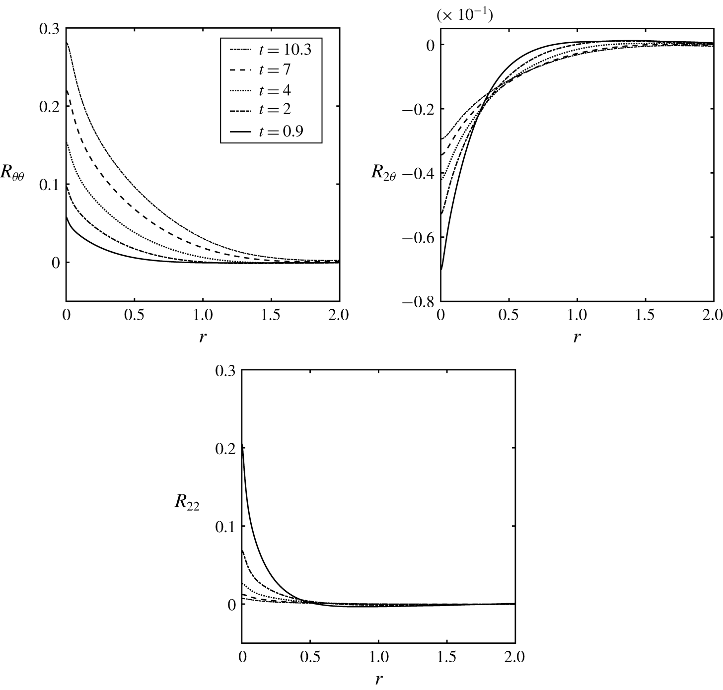
 $R_{\unicode[STIX]{x1D703}\unicode[STIX]{x1D703}}$,
 $R_{2\unicode[STIX]{x1D703}}$ and
 $R_{22}$, respectively, reduce to scalar variance
 $\overline{\unicode[STIX]{x1D703}^{2}}$, transverse scalar flux
 $\overline{u_{2}\unicode[STIX]{x1D703}}$ and variance of transverse fluctuations
 $\overline{u_{2}^{2}}$, i.e.
 $$\begin{eqnarray}\displaystyle & \displaystyle R_{\unicode[STIX]{x1D703}\unicode[STIX]{x1D703}}(\boldsymbol{r}=0,t)=\overline{\unicode[STIX]{x1D703}^{2}}(t), & \displaystyle\end{eqnarray}$$
 $$\begin{eqnarray}\displaystyle & \displaystyle R_{2\unicode[STIX]{x1D703}}(\boldsymbol{r}=0,t)=\overline{u_{2}\unicode[STIX]{x1D703}}(t), & \displaystyle\end{eqnarray}$$
 $$\begin{eqnarray}\displaystyle & \displaystyle R_{22}(\boldsymbol{r}=0,t)=\overline{u_{2}^{2}}(t). & \displaystyle\end{eqnarray}$$
If we finally employ (4.13)–(4.15) into the latter definitions, we obtain the turbulent scaling laws for the one-point quantities as
 $$\begin{eqnarray}\displaystyle & \displaystyle \overline{\unicode[STIX]{x1D703}^{2}}\propto (t+t_{0})^{2n+m}, & \displaystyle\end{eqnarray}$$
 $$\begin{eqnarray}\displaystyle & \displaystyle \overline{u_{2}\unicode[STIX]{x1D703}}\propto (t+t_{0})^{2n-1+m}, & \displaystyle\end{eqnarray}$$
 $$\begin{eqnarray}\displaystyle & \displaystyle \overline{u_{2}^{2}}\propto (t+t_{0})^{2n-2+m}, & \displaystyle\end{eqnarray}$$
and, in general, employing isotropy for the velocities we obtain
 $$\begin{eqnarray}\overline{u^{2}}=\overline{u_{1}^{2}}=\overline{u_{2}^{2}}=\overline{u_{3}^{2}}\propto (t+t_{0})^{2n-2+m}.\end{eqnarray}$$
It should be noted that the Lie symmetry yields the interrelation among the various scaling exponents, as it leads to a connection between the temporal scaling of the velocity and scalar variance. However, the actual values for scaling exponents cannot be obtained alone from the symmetry. Further information is needed on how the large scales have been initialized for the DNS, which is equivalent to knowledge of the integral invariants, such as Batchelor’s or Loitsianskii’s integrals, which are invariants with respect to time  $t$.
From the scaled variable  $\tilde{\boldsymbol{r}}$ in (4.12), we may derive the temporal development of the integral length scale as (Rotta Reference Rotta1972; Oberlack Reference Oberlack2000b)
 $$\begin{eqnarray}\ell _{t}=\int _{0}^{\infty }f(r,t)\,\text{d}r,\end{eqnarray}$$
where  $f$ is the normalised two-point longitudinal velocity correlation function for isotropic turbulence introduced by von Kármán & Howarth (Reference von Kármán and Howarth1938). Substituting the similarity variables (4.12) and (4.15) into (4.28) we find
 $$\begin{eqnarray}\ell _{t}\propto (t+t_{0})^{n}.\end{eqnarray}$$
Finally, it is worth noting that, if the similarity variables are derived correctly, they should turn the governing equations to a reduced self-similar form (where only self-similar variables appear after the reduction, rather similar to the reduction of the boundary layer equations to the Blasius equation). If we substitute the above-derived similarity solutions (4.12)–(4.20) based on the symmetry analysis into the governing equations (3.16)–(3.18) this yields the following reduced self-similar form of the TPC equations:
 $$\begin{eqnarray}\displaystyle & \displaystyle (2n+m)\tilde{R}_{\unicode[STIX]{x1D703}\unicode[STIX]{x1D703}}-n\tilde{r}_{k}\frac{\unicode[STIX]{x2202}\tilde{R}_{\unicode[STIX]{x1D703}\unicode[STIX]{x1D703}}}{\unicode[STIX]{x2202}\tilde{r}_{k}}+2\unicode[STIX]{x1D6E4}\tilde{R}_{2\unicode[STIX]{x1D703}}-\frac{\unicode[STIX]{x2202}\tilde{R}_{(\unicode[STIX]{x1D703}k)\unicode[STIX]{x1D703}}}{\unicode[STIX]{x2202}\tilde{r}_{k}}-\frac{\unicode[STIX]{x2202}\tilde{R}_{\unicode[STIX]{x1D703}(\unicode[STIX]{x1D703}k)}}{\unicode[STIX]{x2202}\tilde{r}_{k}}=0, & \displaystyle\end{eqnarray}$$
 $$\begin{eqnarray}\displaystyle & \displaystyle (2n+m-1)\tilde{R}_{2\unicode[STIX]{x1D703}}-n\tilde{r}_{k}\frac{\unicode[STIX]{x2202}\tilde{R}_{2\unicode[STIX]{x1D703}}}{\unicode[STIX]{x2202}\tilde{r}_{k}}+2\unicode[STIX]{x1D6E4}\tilde{R}_{22}-\frac{\unicode[STIX]{x2202}\widetilde{\overline{p\unicode[STIX]{x1D703}}}}{\unicode[STIX]{x2202}\tilde{r}_{2}}-\frac{\unicode[STIX]{x2202}\tilde{R}_{(2k)\unicode[STIX]{x1D703}}}{\unicode[STIX]{x2202}\tilde{r}_{k}}-\frac{\unicode[STIX]{x2202}\tilde{R}_{2(\unicode[STIX]{x1D703}k)}}{\unicode[STIX]{x2202}\tilde{r}_{k}}=0, & \displaystyle\end{eqnarray}$$
 $$\begin{eqnarray}\displaystyle & \displaystyle (2n+m-2)\tilde{R}_{22}-n\tilde{r}_{k}\frac{\unicode[STIX]{x2202}\tilde{R}_{22}}{\unicode[STIX]{x2202}\tilde{r}_{k}}-\frac{\unicode[STIX]{x2202}\widetilde{\overline{pu_{2}}}}{\unicode[STIX]{x2202}\tilde{r}_{2}}-\frac{\unicode[STIX]{x2202}\widetilde{\overline{u_{2}p}}}{\unicode[STIX]{x2202}\tilde{r}_{2}}-\frac{\unicode[STIX]{x2202}\tilde{R}_{(2k)2}}{\unicode[STIX]{x2202}\tilde{r}_{k}}-\frac{\unicode[STIX]{x2202}\tilde{R}_{2(2k)}}{\unicode[STIX]{x2202}\tilde{r}_{k}}=0, & \displaystyle\end{eqnarray}$$
which confirms the correctness of the derived self-similar solutions. In the next section, the derived theoretical results (4.12)–(4.15) and (4.24)–(4.27) are also validated against the DNS data.
5 Validation of scaling laws
5.1 Details of the direct numerical simulations
We compare the derived theoretical solutions (4.12)–(4.15) and (4.24)–(4.27) based on the symmetry analysis against the highly resolved DNS results of decaying homogeneous isotropic turbulence, performed by Gauding et al. (Reference Gauding, Goebbert, Hasse and Peters2015, Reference Gauding, Danaila and Varea2017, Reference Gauding, Wang, Goebbert, Boded, Danaila and Vareaa2019). While more details can be found in these references, we only briefly describe the details of their DNS code, which solved the incompressible Navier–Stokes equations (2.22) in a triply periodic cubic box with size  $2\unicode[STIX]{x03C0}$ by a pseudo-spectral method. The initial field was generated in the spectral domain and obeyed a prescribed energy spectrum of the Batchelor–Proudman type (Batchelor & Proudman Reference Batchelor and Proudman1956), i.e.
 $$\begin{eqnarray}E(\unicode[STIX]{x1D705},0)\propto \unicode[STIX]{x1D705}^{4}\exp \bigg[-2\left(\frac{\unicode[STIX]{x1D705}}{\unicode[STIX]{x1D705}_{p}}\right)^{2}\bigg],\end{eqnarray}$$
where the large-scale properties ( $k\rightarrow 0$) of
 $E(k)\propto \unicode[STIX]{x1D705}^{4}$ were considered, which leads to the following known temporal evolution (Loitsianskii Reference Loitsianskii1945):
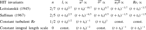
 $$\begin{eqnarray}l_{t}\propto (t+t_{0})^{2/7},\quad \overline{u^{2}}\propto (t+t_{0})^{-10/7},\quad Re_{t}\propto (t+t_{0})^{-3/7}.\end{eqnarray}$$
To ensure an appropriate resolution of all scales, Gauding et al. (Reference Gauding, Danaila and Varea2017, Reference Gauding, Wang, Goebbert, Boded, Danaila and Vareaa2019) have used a grid resolution of  $4096^{3}$ points in their DNS. Additionally, a resolution condition of
 $k_{max}\unicode[STIX]{x1D702}>1$ has been maintained for all cases to accurately compute the high-order statistics. Further, they defined an initial Reynolds number
 $$\begin{eqnarray}\mathit{Re}_{\ast }=\frac{u_{\ast }^{\prime }}{k_{p}\unicode[STIX]{x1D708}}\end{eqnarray}$$
to describe the initial state of freely decaying turbulence. Here,  $k_{p}=15$ is the wavenumber at which the maximum of the initial spectrum
 $E(\unicode[STIX]{x1D705},0)$ occurs,
 $\unicode[STIX]{x1D708}$ is the kinematic viscosity with
 $\unicode[STIX]{x1D708}=1.82\times 10^{-4}$, and an initial turbulence intensity
 $u_{\ast }^{\prime }=2.58$ is specified to obtain an initial turbulent Reynolds number of
 $\mathit{Re}_{\ast }\simeq 945$. With this, they performed ensemble averaging over all grid points in the computational domain, and over three statistically independent realizations of the DNS (Gauding et al. Reference Gauding, Wang, Goebbert, Boded, Danaila and Vareaa2019). With this, statistics have been computed based on more than 200 billion grid points.
For the analysis of turbulent mixing, an additional advection–diffusion equation for the scalar fluctuations, i.e. (3.4), was also solved. Gauding et al. (Reference Gauding, Wang, Goebbert, Boded, Danaila and Vareaa2019) considered a Schmidt number of unity, meaning that the kinematic viscosity  $\unicode[STIX]{x1D708}$ equals the molecular diffusivity
 $\unicode[STIX]{x1D6FC}$. They also imposed a uniform mean scalar gradient
 $\unicode[STIX]{x1D6E4}$ on the scalar field. As noted in Gauding et al. (Reference Gauding, Wang, Goebbert, Boded, Danaila and Vareaa2019), in this configuration, the velocity field is decaying while the scalar field is subject to a continuous injection of energy at the large scales. This flow configuration is similar to those studied experimentally by Warhaft (Reference Warhaft2000) and Bahri et al. (Reference Bahri, Arwatz, George, Mueller and Hultmark2015). It should be highlighted that our theoretical solutions do not contradict the assumption of a high Schmidt number. The effects of Schmidt numbers are essentially profound on the small-scale turbulence (i.e. the separation between the Kolmogorov scale
 $\unicode[STIX]{x1D702}_{k}$ and the Corrsin–Obukhov scale
 $\unicode[STIX]{x1D702}_{co}$ plays an important role) (see e.g. Warhaft Reference Warhaft2000; Antonia & Orlandi Reference Antonia and Orlandi2003; Sreenivasan Reference Sreenivasan2019). As widely reported in the literature, a gradual evolution of a
 $k^{-1}$ or
 $r^{2}$ roll-off in the viscous convective region is expected as Schmidt number increases, consistent with Batchelor’s predictions (Antonia & Orlandi Reference Antonia and Orlandi2003; Mydlarski Reference Mydlarski2003).
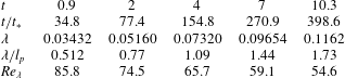
Characteristic parameters of the DNS at different  $t$, which will be used in the next section for the self-similarly analysis, are summarized in table 1 (please see more details in Gauding et al. (Reference Gauding, Wang, Goebbert, Boded, Danaila and Vareaa2019), e.g. table 2). We need to highlight that, in decaying isotropic turbulence, there is not a characteristic time scale (or length scale) that stays constant. Therefore, it has been very common to present the scaling laws in terms of the physical time
 $t$. It is, however, possible to build a constant time scale (length scale) with the parameters of the initial conditions, i.e. the initial turbulence intensity
 $u_{\ast }^{\prime }$ and the peak wavenumber
 $k_{p}$. The time scale is therefore
 $t_{\ast }=1/(k_{p}u_{\ast }^{\prime })$, and
 $1/k_{p}$ is the only relevant length scale as the box size is arbitrary. One could, of course, normalize all quantities with
 $t_{\ast }$ and
 $l_{p}=1/k_{p}$ (see e.g. table 1), but this does not change the behaviour of the scaling laws and invariance.
Basic parameters of the DNS at different  $t$.

5.2 Validation of the scaling laws
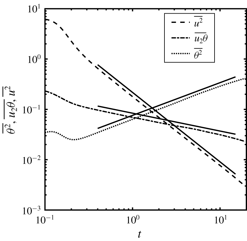
In this subsection, the derived similarity solutions (4.12)–(4.15) and scaling laws (4.24)–(4.27) are validated against the DNS data. First, we establish and verify the results for one-point quantities (4.24)–(4.27), i.e. the scalar variance  $\overline{\unicode[STIX]{x1D703}^{2}}$, the transverse scalar flux
 $\overline{u_{2}\unicode[STIX]{x1D703}}$ and the variance of turbulent fluctuations
 $\overline{u^{2}}$.
The prescribed spectrum at small wavenumbers, i.e.  $E(k)\propto \unicode[STIX]{x1D705}^{4}$, which implies a temporal decay of the form (5.2), leads to
 $$\begin{eqnarray}2n+m\equiv 4/7\end{eqnarray}$$
if compared to the derived decay law (4.27). Therefore, if we replace  $2n+m$ in (4.24) and (4.25), the following scaling laws are obtained
 $$\begin{eqnarray}\displaystyle & \displaystyle \overline{\unicode[STIX]{x1D703}^{2}}\propto (t+t_{0})^{4/7}, & \displaystyle\end{eqnarray}$$
 $$\begin{eqnarray}\displaystyle & \displaystyle \overline{u_{2}\unicode[STIX]{x1D703}}\propto (t+t_{0})^{-3/7}. & \displaystyle\end{eqnarray}$$
Recall that  $n$ is the power-law exponent derived for the integral length scale in (4.29). Once
 $n$ has been determined,
 $m$ can be obtained from the scaling-law relations (e.g. 5.4). If
 $n=2/7$ as for Loitsianskii’s integral (5.2), this gives
 $m=0$, which suggests that the statistical symmetry is presently negligible. The above scaling laws (5.2), (5.5) and (5.6) obtained from the symmetry analysis lead to interesting solutions, as both the variance of fluctuations
 $\overline{u^{2}}$ and the transverse scalar flux
 $\overline{u_{2}\unicode[STIX]{x1D703}}$ decay in time, while the scalar variance
 $\overline{\unicode[STIX]{x1D703}^{2}}$ shows a growing behaviour in time. It should also be noted that in the present setting from the flux vector
 $\overline{u_{i}\unicode[STIX]{x1D703}}$ only
 $\overline{u_{2}\unicode[STIX]{x1D703}}$ is non-zero, as for the other two components
 $u_{i}$ and
 $\unicode[STIX]{x1D703}$ decorrelate.
Prior to the validation of the scaling laws with the DNS, it should be noted that the present scaling laws can be expected to hold only in the intermediate stage of the decay where  $Re_{\unicode[STIX]{x1D706}}$ is sufficiently large and the turbulent kinetic energy, under the assumption of Loitsianskii’s integral, follows
 $\overline{u^{2}}\propto (t+t_{0})^{-10/7}$. All turbulence variances including the scalar variance should eventually decay to vanish at the final stage of the decay, when
 $Re_{t}\rightarrow 0$ and
 $t\rightarrow \infty$ (Batchelor & Townsend Reference Batchelor and Townsend1948; George Reference George1992a). Although, in general, a simple Reynolds-number criterion for the existence of the final period flow cannot be justified, it has been mostly suggested that the final decay period law sets in at approximately
 $Re_{\unicode[STIX]{x1D706}}\ll 15$ (Batchelor & Townsend Reference Batchelor and Townsend1948; George Reference George1992a).
The temporal variation of  $\overline{\unicode[STIX]{x1D703}^{2}}$,
 $\overline{u_{2}\unicode[STIX]{x1D703}}$ and
 $\overline{u^{2}}$ with time
 $t$ from DNS data of Gauding et al. (Reference Gauding, Wang, Goebbert, Boded, Danaila and Vareaa2019). The solid lines are power-law fits to the DNS data:
 $\overline{\unicode[STIX]{x1D703}^{2}}\sim (t+t_{0})^{0.65}$,
 $\overline{u_{2}\unicode[STIX]{x1D703}}\sim (t+t_{0})^{-0.36}$ and
 $\overline{u^{2}}\sim (t+t_{0})^{-1.38}$. The virtual origin of
 $t_{0}=0$ was obtained.

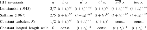
Figure 1 displays the evolutions of  $\overline{\unicode[STIX]{x1D703}^{2}}$,
 $\overline{u_{2}\unicode[STIX]{x1D703}}$ and
 $\overline{u^{2}}$ with time
 $t$, on a double-logarithmic scale, from the DNS results of Gauding et al. (Reference Gauding, Wang, Goebbert, Boded, Danaila and Vareaa2019). It can be observed that all statistical quantities, i.e.
 $\overline{\unicode[STIX]{x1D703}^{2}}$,
 $\overline{u_{2}\unicode[STIX]{x1D703}}$ and
 $\overline{\unicode[STIX]{x1D703}^{2}}$, follow a power law, with exponents that are very close to the analysis prediction in (5.2), (5.5) and (5.6). It should be noted that small deviations from the theoretical scaling exponents and DNS data are to be expected and can be related to the tradeoff between Reynolds number and the DNS box confinement (Ishida, Davidson & Kaneda Reference Ishida, Davidson and Kaneda2006). We do not have an indication from the DNS data that the statistical symmetry (4.6a-n) connected to
 $m$ plays a role here. Hence, in the following we set
 $m=0$.
As noted, the current flow is initialized using Batchelor–Proudman turbulence with  $E(k)\propto \unicode[STIX]{x1D705}^{4}$ for
 $k\rightarrow 0$, which gives rise to
 $n=2/7$. A complete self-similarity requires a constant Reynolds number, which is possible in decaying homogeneous isotropic turbulence only under the condition that the turbulent kinetic energy and integral length scale decay as
 $\overline{u^{2}}\propto t^{-1}$ and
 $l_{t}\propto t^{1/2}$, respectively (see e.g. Oberlack Reference Oberlack2002). However, such decay laws are essentially never perfectly observed from experimental or DNS data (Mohamed & Larue Reference Mohamed and Larue1990; Oberlack Reference Oberlack2002). In table 2, we present the scaling laws (4.24)–(4.29) of a passive scalar with a constant mean scalar gradient in decaying isotropic turbulence employing various different invariants.
It should be noted that the time  $t_{0}$ is left undetermined from the theory. It may well be influenced by the initial conditions, as the time until similarity has been achieved may strongly depend on the initial conditions chosen in a DNS.
Now, we turn our attention to the two-point tensors and their self-similar solutions, i.e. (4.13)–(4.15). Figure 2 presents the unscaled TPC tensors  $R_{\unicode[STIX]{x1D703}\unicode[STIX]{x1D703}}(\boldsymbol{r},t)$,
 $R_{2\unicode[STIX]{x1D703}}(\boldsymbol{r},t)$ and
 $R_{22}(\boldsymbol{r},t)$ at different
 $t$. According to (4.12)–(4.15), these tensors comply self-similarity if they are respectively scaled using the power-law functions as given in (4.24)–(4.27) and the length scale following (4.29). As was shown based on the DNS data in figure 1, one-point quantities are found to closely follow these power-law behaviours. Therefore, it is straightforward to normalize the two-point tensors using their one-point quantities, i.e.
 $$\begin{eqnarray}\displaystyle & \displaystyle \tilde{R}_{\unicode[STIX]{x1D703}\unicode[STIX]{x1D703}}(\tilde{\boldsymbol{r}})=\frac{R_{\unicode[STIX]{x1D703}\unicode[STIX]{x1D703}}(\boldsymbol{r},t)}{\overline{\unicode[STIX]{x1D703}^{2}}}, & \displaystyle\end{eqnarray}$$
 $$\begin{eqnarray}\displaystyle & \displaystyle \tilde{R}_{2\unicode[STIX]{x1D703}}(\tilde{\boldsymbol{r}})=\frac{R_{2\unicode[STIX]{x1D703}}(\boldsymbol{r},t)}{\overline{u_{2}\unicode[STIX]{x1D703}}} & \displaystyle\end{eqnarray}$$
and
 $$\begin{eqnarray}\tilde{R}_{22}(\tilde{\boldsymbol{r}})=\frac{R_{22}(\boldsymbol{r},t)}{\overline{u^{2}}},\end{eqnarray}$$
with
 $$\begin{eqnarray}\tilde{\boldsymbol{r}}=\frac{\boldsymbol{r}}{(t+t_{0})^{n}}.\end{eqnarray}$$
The exponent  $n$, which leads to the complete self-similarity of the TPC tensors (e.g. (4.13)–(4.15)), can be estimated from the temporal evolution of the integral scale as derived in (4.29). The temporal evolution of
 $\ell _{t}$ is provided in figure 3, where it is found that
 $\ell _{t}$ closely follows (4.29) with
 $n=0.29$ and
 $t_{0}=0$, which is close to the theoretical value of
 $n=2/7$. Figure 4 presents the two-point tensors shown in figure 2, but now scaled based on the scaling laws obtained by the symmetry analysis (5.7)–(5.10) and the integral scale in (4.29). Note that here we used the DNS data for normalization of the two-point tensors. It can be observed that the collapse of the profiles for the scaled two-point tensors is very good, which verifies the accuracy of the derived scaling laws and applied analysis.
The unscaled TPC tensors.
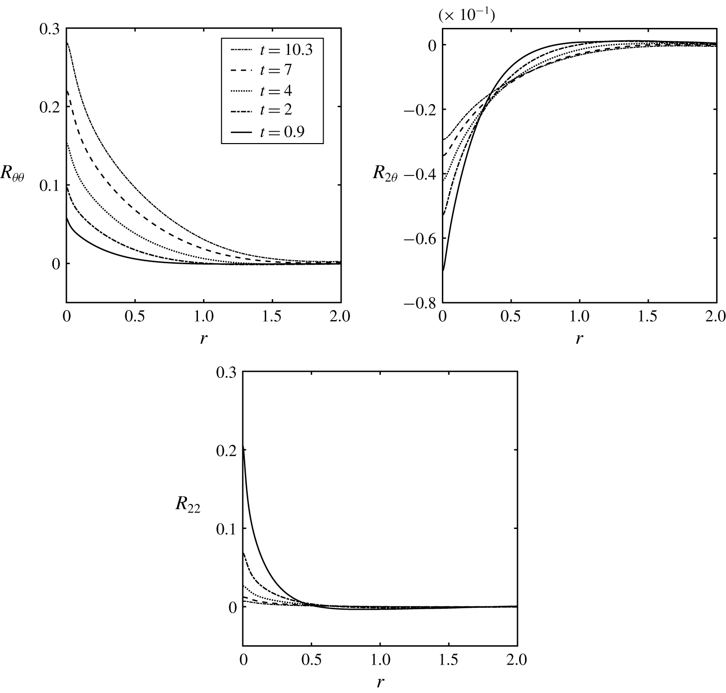
The variation of different length scales with  $t$. The top solid line is a power-law fit to the DNS data for the integral scale
 $\ell _{t}\sim (t+t_{0})^{0.29}$ with
 $t_{0}=0$. The other solid lines represent power-law fits to the Taylor microscale
 $\unicode[STIX]{x1D706}\sim (t+t_{0})^{0.49}$ and the scalar Taylor microscale
 $\unicode[STIX]{x1D706}_{\unicode[STIX]{x1D703}}\sim (t+t_{0})^{0.49}$, where
 $\unicode[STIX]{x1D706}$ and
 $\unicode[STIX]{x1D706}_{\unicode[STIX]{x1D703}}$ follow the same square-root power law and are identified by a single solid line, and the Kolmogorov length scale
 $\unicode[STIX]{x1D702}_{k}\sim (t+t_{0})^{0.59}$ with
 $t_{0}=0$.
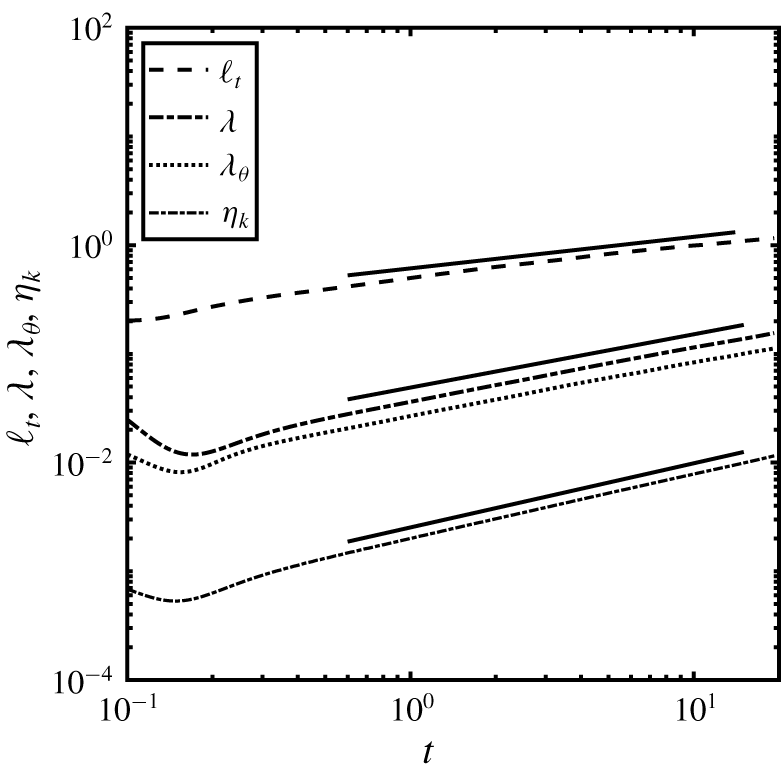


In the literature (see e.g. George Reference George1992a,Reference Georgeb; Bahri et al. Reference Bahri, Arwatz, George, Mueller and Hultmark2015; Gauding et al. Reference Gauding, Wang, Goebbert, Boded, Danaila and Vareaa2019) it has been suggested that the TPC may not scale on the integral length scale  $\ell _{t}$ but instead on the Kolmogorov length scale
 $\unicode[STIX]{x1D702}_{k}$, the Taylor microscale
 $\unicode[STIX]{x1D706}$ or rather the scalar Taylor microscale
 $\unicode[STIX]{x1D706}_{\unicode[STIX]{x1D703}}$. With the relations above, we find for the Kolmogorov length scale
 $\unicode[STIX]{x1D702}_{k}$,
 $$\begin{eqnarray}\unicode[STIX]{x1D702}_{k}\equiv \unicode[STIX]{x1D708}^{3/4}/\langle \unicode[STIX]{x1D716}\rangle ^{1/4}\propto (t+t_{0})^{-(1/4)(2n-3+m)},\end{eqnarray}$$
for the Taylor microscale,  $\unicode[STIX]{x1D706}$,
 $$\begin{eqnarray}\unicode[STIX]{x1D706}\equiv [15\unicode[STIX]{x1D708}\overline{u^{2}}/\langle \unicode[STIX]{x1D716}\rangle ]^{1/2}\propto (t+t_{0})^{1/2},\end{eqnarray}$$
and for the scalar Taylor microscale,  $\unicode[STIX]{x1D706}_{\unicode[STIX]{x1D703}}$,
 $$\begin{eqnarray}\unicode[STIX]{x1D706}_{\unicode[STIX]{x1D703}}\equiv [6\unicode[STIX]{x1D6FC}\overline{\unicode[STIX]{x1D703}^{2}}/\langle \unicode[STIX]{x1D716}_{\unicode[STIX]{x1D703}}\rangle ]^{1/2}\propto (t+t_{0})^{1/2},\end{eqnarray}$$
where  $\langle \unicode[STIX]{x1D716}\rangle$ and
 $\langle \unicode[STIX]{x1D716}_{\unicode[STIX]{x1D703}}\rangle$ are, respectively, the mean dissipation of kinetic energy and the mean scalar dissipation. The above-mentioned theoretical scalings are validated against DNS data in figure (3). Additionally, the similarity of the TPC tensors using
 $\unicode[STIX]{x1D706}$ and
 $\unicode[STIX]{x1D706}_{\unicode[STIX]{x1D703}}$ and
 $\unicode[STIX]{x1D702}_{k}$ (5.11)–(5.13) is tested in figures 5 and 6. It can be observed that the profiles depart widely from one another in a significant range of intermediate and large scales. This departure is more apparent when
 $\unicode[STIX]{x1D702}_{k}$ was used. This is in agreement with the observation of Gauding et al. (Reference Gauding, Wang, Goebbert, Boded, Danaila and Vareaa2019) that the normalized TPC tensor of all turbulent quantities and
 $\unicode[STIX]{x1D702}_{k}$ is not completely self-similar for almost all ranges of scales.


6 Summary and conclusions
In this work, Lie group symmetry analysis was considered to derive the scaling laws and similarity solutions. The flow of interest was a passive scalar advected by a statistically homogeneous isotropic and incompressible turbulent velocity field, while a uniform mean gradient  $\unicode[STIX]{x1D6E4}$ is imposed on the scalar field in the cross-stream direction. We applied symmetry theory to a system of two-point correlation (TPC) equations for the scalar and velocity fluctuations. As a result, a set of different invariant (self-similar) solutions – the TPC tensors of the passive scalar and fluctuating velocity scalar – has been derived. In addition, the scaling laws for one-point quantities of the scalar variance
 $\overline{\unicode[STIX]{x1D703}^{2}}$, the transverse scalar flux
 $\overline{u_{2}\unicode[STIX]{x1D703}}$ and the variance of turbulent fluctuations
 $\overline{u^{2}}$ have been constructed. A direct connection between the derived scaling laws and symmetries was established, which was the consequence of the symmetry breaking induced by the constant mean scalar gradient. Highly resolved direct numerical simulation (DNS) of decaying homogeneous isotropic turbulence has been employed to verify the validity of the new scaling laws. A very good agreement between the DNS and the derived scaling laws and similarity solutions was found.
Acknowledgements
H.S. acknowledges the financial support of the Alexander von Humboldt Foundation. The authors greatly appreciate Dr M. Gauding for providing his DNS data.
Declaration of interests
The authors report no conflict of interest.
Appendix A
In this appendix, we present the symmetry results and the subsequent scaling laws in homogeneous turbulence imposed by both a uniform mean temperature gradient (i.e.  $\overline{\unicode[STIX]{x1D6E9}}=\unicode[STIX]{x1D6E4}x_{2}$) and a uniform mean velocity gradient (
 $\overline{U}_{1}=\unicode[STIX]{x1D6F6}x_{2}$). As we assume large-scale effects, we set
 $\unicode[STIX]{x1D708}=0$ and
 $\unicode[STIX]{x1D6FC}=0$. Thus (2.22) and (2.28) together with (3.1) and
 $\overline{\unicode[STIX]{x1D6E9}}=\unicode[STIX]{x1D6E4}x_{2}$ and
 $\overline{U}_{1}=\unicode[STIX]{x1D6F6}x_{2}$ change to the following relations for the scalar fluctuations
 $\unicode[STIX]{x1D703}$ and velocity fluctuations
 $u_{i}$:
 $$\begin{eqnarray}\frac{\unicode[STIX]{x2202}\unicode[STIX]{x1D703}}{\unicode[STIX]{x2202}t}+u_{k}\frac{\unicode[STIX]{x2202}\unicode[STIX]{x1D703}}{\unicode[STIX]{x2202}x_{k}}+\unicode[STIX]{x1D6F6}x_{2}\frac{\unicode[STIX]{x2202}\unicode[STIX]{x1D703}}{\unicode[STIX]{x2202}x_{1}}+u_{2}\unicode[STIX]{x1D6E4}=0,\end{eqnarray}$$
and
 $$\begin{eqnarray}\frac{\unicode[STIX]{x2202}u_{i}}{\unicode[STIX]{x2202}t}+u_{k}\frac{\unicode[STIX]{x2202}u_{i}}{\unicode[STIX]{x2202}x_{k}}+\unicode[STIX]{x1D6F6}x_{2}\frac{\unicode[STIX]{x2202}u_{i}}{\unicode[STIX]{x2202}x_{1}}+u_{2}\unicode[STIX]{x1D6F6}\unicode[STIX]{x1D6FF}_{i1}+\frac{\unicode[STIX]{x2202}p}{\unicode[STIX]{x2202}x_{i}}=0,\quad \frac{\unicode[STIX]{x2202}u_{k}}{\unicode[STIX]{x2202}x_{k}}=0.\end{eqnarray}$$
A key point here is that both the constant mean temperature gradient  $\unicode[STIX]{x1D6E4}$ and the constant mean velocity gradient
 $\unicode[STIX]{x1D6F6}$ induce symmetry breakings. This is directly obtained by implementing the generic multi-parameter group (4.3a-h) into (A 1) and (A 2). After dividing by
 $\exp (-a_{\unicode[STIX]{x1D703}}+a_{2})$ and
 $\exp (a_{1}-2a_{2})$, we respectively obtain
 $$\begin{eqnarray}\frac{\unicode[STIX]{x2202}\unicode[STIX]{x1D703}^{\ast }}{\unicode[STIX]{x2202}t^{\ast }}+u_{k}^{\ast }\frac{\unicode[STIX]{x2202}\unicode[STIX]{x1D703}^{\ast }}{\unicode[STIX]{x2202}x_{k}^{\ast }}+\unicode[STIX]{x1D6F6}x_{2}^{\ast }\frac{\unicode[STIX]{x2202}\unicode[STIX]{x1D703}^{\ast }}{\unicode[STIX]{x2202}x_{1}^{\ast }}\exp (-a_{2})+u_{2}^{\ast }\unicode[STIX]{x1D6E4}\exp (a_{\unicode[STIX]{x1D703}}-a_{1})=0\end{eqnarray}$$
and
 $$\begin{eqnarray}\frac{\unicode[STIX]{x2202}u_{i}^{\ast }}{\unicode[STIX]{x2202}t^{\ast }}+u_{k}^{\ast }\frac{\unicode[STIX]{x2202}u_{i}^{\ast }}{\unicode[STIX]{x2202}x_{k}^{\ast }}+\left[\unicode[STIX]{x1D6F6}x_{2}^{\ast }\frac{\unicode[STIX]{x2202}u_{i}^{\ast }}{\unicode[STIX]{x2202}x_{1}^{\ast }}+u_{2}^{\ast }\unicode[STIX]{x1D6F6}\unicode[STIX]{x1D6FF}_{i1}\right]\exp (-a_{2})+\frac{\unicode[STIX]{x2202}p^{\ast }}{\unicode[STIX]{x2202}x_{i}^{\ast }}=0,\quad \frac{\unicode[STIX]{x2202}u_{k}^{\ast }}{\unicode[STIX]{x2202}x_{k}^{\ast }}=0.\end{eqnarray}$$
We observe that both  $\unicode[STIX]{x1D6E4}$ and
 $\unicode[STIX]{x1D6F6}$ are symmetry breaking and therefore the scaling symmetries of space and temperature have to combine to a single symmetry, i.e.
 $$\begin{eqnarray}a_{\unicode[STIX]{x1D703}}=a_{1},\end{eqnarray}$$
and the scaling symmetries of time vanishes, i.e.
 $$\begin{eqnarray}a_{2}=0.\end{eqnarray}$$
If we replace  $a_{\unicode[STIX]{x1D703}}=a_{1}$ and
 $a_{2}=0$ in the corresponding characteristic equations for the invariant solutions, i.e. (4.11), this leads to the following set of invariants:
 $$\begin{eqnarray}\displaystyle & \displaystyle \tilde{\boldsymbol{r}}=\frac{\boldsymbol{r}}{\exp (qt)}, & \displaystyle\end{eqnarray}$$
 $$\begin{eqnarray}\displaystyle & \displaystyle \tilde{R}_{\unicode[STIX]{x1D703}\unicode[STIX]{x1D703}}(\tilde{\boldsymbol{r}})=\frac{R_{\unicode[STIX]{x1D703}\unicode[STIX]{x1D703}}(\boldsymbol{r},t)}{\exp [(2q+p)t]}, & \displaystyle\end{eqnarray}$$
 $$\begin{eqnarray}\displaystyle & \displaystyle \tilde{R}_{2\unicode[STIX]{x1D703}}(\tilde{\boldsymbol{r}})=\frac{R_{2\unicode[STIX]{x1D703}}(\boldsymbol{r},t)}{\exp [(2q+p)t]} & \displaystyle\end{eqnarray}$$
and
 $$\begin{eqnarray}\tilde{R}_{22}(\tilde{\boldsymbol{r}})=\frac{R_{22}(\boldsymbol{r},t)}{\exp [(2q+p)t]},\end{eqnarray}$$
where
 $$\begin{eqnarray}q=\frac{a_{1}}{a_{3}}\end{eqnarray}$$
and
 $$\begin{eqnarray}p=\frac{a_{s}}{a_{3}}.\end{eqnarray}$$
With this, the following exponential turbulent scaling laws for the one-point quantities
 $$\begin{eqnarray}\displaystyle & \displaystyle \overline{\unicode[STIX]{x1D703}^{2}}\propto \exp [(2q+p)t], & \displaystyle\end{eqnarray}$$
 $$\begin{eqnarray}\displaystyle & \displaystyle \overline{u_{2}\unicode[STIX]{x1D703}}\propto \exp [(2q+p)t] & \displaystyle\end{eqnarray}$$
and
 $$\begin{eqnarray}\overline{u_{2}^{2}}=\overline{u^{2}}\propto \exp [(2q+p)t]\end{eqnarray}$$
are obtained.