1 INTRODUCTION
It is acknowledged that evaluations of economic theory often depend on statistical inference on linear functionals in the nonparametric models. In the related literature, the associated discussions mainly focus on the pointwise testing procedures of these functionals by providing confidence intervals (CIs) evaluated at finite grid points. The pointwise CIs that ignore the guiding information on other parts of the support can lead to spurious statistical significance and misguide economic decisions, calling upon the alternative uniform confidence bands (UCBs) whose validity holds across the compact support (or a compact subset). Such concerns motivate us to develop uniform inference procedures for a broad class of nonparametric panel models.
To be specific, we consider a nonparametric panel data model with one-way fixed effects,
 $$ \begin{align*} y_{it}={\gamma_{i}}+g\left(x_{it}\right)+\epsilon_{it},~~i\in[n],~~t\in[T], \end{align*} $$
in which
 $g(\cdot )$
is an unknown function that belongs to the function class
 $\mathcal {G}$
,
 $x_{it}\in \mathcal {X}\subseteq \mathbb {R}^{d}$
is a d-dimensional vector of covariates, which follow arbitrary types of stationary or nonstationary dependence (e.g., stationary mixingale, mildly stationary (Phillips and Magdalinos, Reference Phillips and Magdalinos2007), unit root, or local-to-unity (Phillips, Reference Phillips1987) processes),
 $\gamma _{i}$
denotes the individual fixed effect, and
 $\epsilon _{it}$
is an idiosyncratic error component.
In order to introduce the UCBs for the unknown function
 $g(x)$
, we first evaluate the upper bounds for estimating
 $g(x)$
and its functionals (e.g., derivatives) based on the panel within-group sieve estimator
 $\widehat {g}(\cdot )$
that will be introduced in Section 2; that is, we bound
 $$ \begin{align*} &\sup_{x\in{\mathcal{C}}}\left\vert \widehat{g}(x)-g(x)\right\vert~\text{and}~\sup_{x\in{\mathcal{C}}}\left\vert \partial^{j}\widehat{g}(x)-\partial^{j}g(x)\right\vert, \end{align*} $$
in which
 $\partial ^{j}\widehat {g}(\cdot )$
represents the jth-order partial derivatives of
 $g(\cdot )$
in terms of x and
 $\mathcal {C}$
is any compact subset of the support,
 $\mathcal {X}$
. Specifically, we provide the sup-norm upper bound for our sieve estimator
 $\widehat {g}(\cdot )$
. Next, we establish the strong Gaussian approximation for the estimated linear functionals of
 $g(x)$
in our panel model under various types of intertemporal dependence. Finally, we show the uniform probability coverage of the sieve score bootstrap UCBs for the linear functionals of
 $g(x)$
under primitive conditions.
In the asymptotic development, we approximate the empirical process by a Gaussian process of a growing dimension. The strong approximation allows us to perform inference across any compact subset
 $\mathcal {C}$
and to test for various functionals of
 $g(\cdot )$
, which is infeasible given the pointwise limit theory. Our article extends Yurinskii’s coupling to a nonparametric fixed-effects panel data model that allows for arbitrary types of stationary or nonstationary processes. To the best of our knowledge, the present article belongs to the first of including the near unit root process in establishing the coupling principle.
Moreover, this article extends the proposed framework to the nonparametric panel data model that incorporates both individual and time fixed effects,
 $\gamma _i$
and
 $f_t$
. We require that the considered regressors be stationary mixingale but allow the time fixed effects,
 $f_t$
, to have any intertemporal dependence. We extend our strong approximation and bootstrapped UCBs to the two-way fixed-effects panel model and prove the validity.
Extensive simulations compare the performance of the bootstrapping UCBs with pointwise CIs and verify the good behavior of the bootstrapping UCBs in the finite sample. In particular, the widths of the pointwise CIs are narrower than UCBs, showing that severe size distortions of rejecting the uniform null hypotheses can arise when the empirical analysis is based on pointwise CIs. Various specifications are examined, including the one-way fixed-effects panel data model with a univariate regressor, the partial linear panel modelFootnote 1 and the two-way fixed-effects panel model. Also, sensitivity analysis is conducted regarding the order of sieve expansion, showing the robust uniform size controls of our UCBs.
In addition, we present an empirical example to illustrate the usefulness of UCBs for analyzing income–consumption dynamics. We provide the bootstrapping UCBs and pointwise CIs for consumption concerning income shocks and asset holdings. The empirical results show that the UCBs of each covariate are wider than its pointwise CIs, coinciding with the findings of numerical simulations.
This article is related to three strands of literature. First, the article contributes to the literature on coupling and high-dimensional central limit theorems (CLTs). For the independent random vectors, the high-dimensional CLTs and bootstrap theory are provided in Chernozhukov, Chetverikov, and Kato (Reference Chernozhukov, Chetverikov and Kato2014). Moreover, high-dimensional CLTs are discussed in the case of time series and network/spatial data (Li and Liao, Reference Li and Liao2020; Kurisu, Kato, and Shao, Reference Kurisu, Kato and Shao2024; Li, Liao, and Zhou, Reference Li, Liao and Zhou2024). Our article extends Yurinskii’s coupling principle to the panel data model that incorporates nonstationary processes and provides UCBs for the unknown functionals in a nonparametric panel data model.
Second, the present article contributes to the literature on sieve estimations of the nonstationary time-series models. Due to the wandering behavior of nonstationary processes, the range of a unit root process,
 $\mathcal {X}$
, is expanded to the real number line
 $\mathbb {R}$
, violating the assumption of compact support in much of the literature on sieve estimation. As an alternative, Dong, Gao, and Peng (Reference Dong, Gao and Peng2019) considered the orthogonal Hermite polynomial system defined on the real number line and further established the inference procedures relying on sieve estimations on the unbounded support. To the best of our knowledge, no strong approximation theory or uniform inference procedure is available for the series/sieve estimators that depend on the Hermite polynomial system.
The present article also contributes to the literature on specification testing in the nonparametric panel model. Discussions of estimations and specification tests for nonparametric/semi-nonparametric panel data models that will be introduced later focus more on pointwise asymptotic theory and the Cramér–von Mises test (Su and Lu, Reference Su and Lu2013; Lee, Reference Lee2014). Though econometricians can still achieve consistent specifications via the Cramér–von Mises tests, specific types of tests can generate better power performance against a particular class of alternatives. So, it is essential to apply the test to a suitable setting and examine the panel data sup-test, which remains to be investigated. This article contributes to this field by filling this void.
The structure of the present article is as follows. Section 2 presents our nonparametric panel data model with one-way individual fixed effects and discusses the sieve estimator and its properties. Section 3 derives the uniform limit theory for the sieve estimation. Section 4 provides the sieve score bootstrap UCBs and proves their uniform size controls. Section 5 extends our bootstrapping uniform inference procedure to the nonparametric panel model with two-way fixed effects. Section 6 examines the finite-sample performance of the sieve score bootstrapping UCBs using Monte Carlo simulations. Section 7 applies the uniform inference procedure to empirical data. Section 8 concludes. The Supplementary Material collects all the proofs and additional simulation studies.
In what follows, the
 $\ell _2$
-norm of the vector v is denoted by
 $\Vert v\Vert $
and the operator norm for a matrix M is given by
 $\Vert M \Vert $
. For a matrix-valued function
 $Q(x)$
with
 $x\in \mathcal {X}$
, the notation
 $\Vert Q\Vert _{\mu ,q}:=(\int _{x\in \mathcal {X}}\Vert Q(x)\Vert ^q \mu (x)dx)^{1/q}$
, in which
 $\mu (\cdot )$
is the Lebesgue measure. The space
 $L_2\left (\mathbb {R}, \mu (x)\right )$
represents the class of functions with
 $\Vert Q(x)\Vert _{\mu ,2}<\infty $
. The notation
 $a \lesssim b$
denotes
 $a\leq cb$
for some constant c, while the notation
 $a\lesssim _{p} b$
represents
 $a=O_{p}(b)$
or
 $a=o_{p}(b)$
. The notation
 $a\asymp b$
means that
 $a\lesssim b$
and
 $b\lesssim a$
. The notations
 $\rightarrow _{p}$
and
 $\Rightarrow $
denote convergence in probability and weak convergence. The notation
 $\mathbf {1}_{1\times d}$
refers to a d-dimensional row vector of ones, the notation
 $\mathbf {0}_{d\times 1}$
denotes a d-dimensional column vector of zeros, and the quantity
 $\mathbf {0}_{d\times d}$
represents a
 $d\times d$
matrix of zeros. We use standard notations
 $\mathbb {E}_n[\cdot ]$
,
 $\mathbb {E}_T[\cdot ]$
,
 $\mathbb {E}^{\ast }_T[\cdot ]$
,
 $\mathbb {G}_n[\cdot ],$
and
 $\mathbb {G}_T[\cdot ]$
in the empirical process literature as
 $\mathbb {E}_{n}[f]=(1/n)\sum ^{n}_{i=1}f(w_{i})$
,
 $\mathbb {E}_{T}[f]=(1/a_{T}^2)\sum ^{T}_{t=1}f(w_{t})$
,
 $\mathbb {E}^{\ast }_{T}[f]=(1/T)\sum ^{T}_{t=1}f(w_{t})$
,
 $\mathbb {G}_{n}[f]=(1/\sqrt {n})\sum ^{n}_{i=1}(f(w_{i})-\mathbb {E}(f(w_{i})))$
, and
 $\mathbb {G}_{T}[f]=(1/a_{T})\sum ^{T}_{t=1}(f(w_{t})-\mathbb {E}(f(w_{t})))$
, where
 $a_{T}$
is the stabilization rate (i.e.,
 $a_{T}=\sqrt {T}$
for stationary mixingale case,
 $a_{T}=\sqrt {T^{1-\zeta /2}}$
for mildly stationary case, and
 $a_{T}=\sqrt [4]{T}$
for the unity/local-to-unity case).Footnote
2
Write
 $i\in [n]$
to denote
 $i=1,\ldots ,n$
and use similar notations as
 $t\in [T]$
.
2 MODEL SETUP AND SIEVE ESTIMATION
2.1 Model
We restate the additive nonparametric panel data model with individual fixed effects of the introduction. The dependent variable
 $y_{it}$
is generated according to
 $$ \begin{align} y_{it}={\gamma_{i}}+g\left(x_{it}\right)+\epsilon_{it},~~\mathbb{E}\left[\epsilon_{it}|\{x_{it}\}_{t\in[T]}\right]=0,~~i\in\left[n\right]~\text{and}~t\in\left[T\right], \end{align} $$
in which
 $g(\cdot )$
is an unknown function of the space
 $\mathcal {G}$
,
 $x_{it}$
is a d-dimensional vector of covariates taking values in the set
 $\mathcal {X}\subseteq \mathbb {R}^{d}$
,
 $\gamma _{i}$
denotes the individual fixed effect that is correlated with regressors
 $x_{it}$
, and
 $\epsilon _{it}$
is an error term. We discuss a panel model with a large cross-sectional dimension n but impose no restrictions on the time-series dimension T; that is, T stays fixed or grows to infinity.
In equation (1), we impose cross-sectional independence for variates
 $(x^{\prime }_{it},\epsilon _{it})^{\prime }$
but incorporate various forms of time-series correlations for
 $(x^{\prime }_{it},\epsilon _{it})^{\prime }$
. In particular, the error
 $\epsilon _{it}$
is a stationary mixingale that forms a general class of time-series behaviors, including martingale differences, linear processes, and various types of mixing and near-epoch-dependent processes as special cases (Li and Liao, Reference Li and Liao2020). Moreover, the covariate
 $x_{it}$
follows an arbitrary type of stationary or nonstationary process which incorporates stationary mixingale, mildly stationary, unit root, or local-to-unit root process. Specifically, we impose the following conditions on
 $x_{it}$
and
 $\epsilon _{it}$
to summarize the requirements.
Assumption 1. For each
 $i\in [n]$
, the variates
 $\upsilon _{it}=\left (x^{\prime }_{it},\epsilon _{it}\right )^{\prime }$
that satisfy equation (1) are mutually independent across
 $i\in \left [n\right ]$
. Regression errors
 $\left \{\epsilon _{it}\right \}$
satisfy the uniform upper bound condition:
 $\sup _{x\in \mathcal {X}}\mathbb {E}\left [\left \vert \epsilon _{it}\right \vert {}^m| {\{x_{it}\}_{t\in [T]}}\right ]\lesssim 1$
, for some
 $m>6$
.
Assumption 2. For each
 $i\in \left [n\right ]$
, the variates
 $\{\upsilon _{it}\}$
follow a
 $(d+1)$
-dimensional stationary
 $L_q$
-mixingale array (
 $q\geq 3$
) with respect to a filtration
 $\{\mathcal {F}_{i,t}\}$
that satisfies the following conditions: for any
 $l\geq 0$
, with
 $\upsilon _{T,it}:=\upsilon _{it}/\sqrt {T}$
and F as a cumulative distribution function (CDF) for
 $\{\upsilon _{it}\}$
, it follows that
 $$ \begin{align} \left\Vert \mathbb{E}\left[\left.\upsilon_{T,it}^{}\right\vert \mathcal{F}_{i,t-l}\right]\right\Vert{}_{q}\leq c_{i,t}\cdot\nu_{l},~\left\Vert \upsilon_{T,it}^{}- \mathbb{E}\left[\left.\upsilon_{T,it}^{}\right\vert \mathcal{F}_{i,t+l}\right]\right\Vert{}_{q}\leq c_{i,t}\cdot\nu_{l+1}, \end{align} $$
with
 $\left \Vert \upsilon \right \Vert {}_q=(\mathbb {E}\left \Vert \upsilon \right \Vert {}^q)^{1/q}$
for some positive sequence
 $\overline {c}_{i}$
,
 $\sup _{t\in \left [T\right ]}\left \vert c_{i,t}\right \vert \leq \overline {c}_i/\sqrt {T}=O(1)$
for each
 $i\in \left [n\right ]$
Footnote
3
and
 $\sum ^{\infty }_{l=1}\nu _l<\infty $
. Assume that
 $v_{it}$
has sub-Gaussian tails.
Assumption 3. For each
 $i\in \left [n\right ]$
, the error
 $\{\epsilon _{it}\}$
follows the formulation of a mixingale process in Assumption 2, while the univariate (
 $d=1$
) regressor
 $\{x_{it}\}$
follows a near unit root processFootnote
4
as
 $x_{it}=(1+C/T^{\zeta })x_{i,t-1}+u_{x,it}$
in which
 $\zeta \in (0,1]$
and
 $u_{x,it}\sim \text {iid}(0,\sigma _{x}^{2})$
. The scalar quantity C is any constant scalar value when
 $\zeta =1$
(unity/local-to-unity; Phillips, Reference Phillips1987) while is negative when
 $\zeta \in (0,1)$
(mildly stationary; Phillips and Magdalinos, Reference Phillips and Magdalinos2007).
Several remarks are given in order. First, in the present article, we impose cross-sectional independence across i to facilitate the strong approximation in the later discussions. The attempt to relax the restrictions of cross-sectional independence in
 $x_{it}$
is meaningful and is left for future studies. Second, Assumptions 2 and 3 take into account two cases for
 $\{x_{it}\}$
and
 $\left \{\epsilon _{it}\right \}$
. In Assumption 2, the covariates
 $\{x_{it}\}$
are stationary mixingales and uncorrelated with the instantaneous error
 $\{\epsilon _{it}\}$
, similar as the setting of regressors and error term in Li and Liao (Reference Li and Liao2020). While in Assumption 3, the covariate
 $\left \{x_{it}\right \}$
is a scalar near unit root process (
 $d=1$
) whose autoregressive root lies inside a shrinking neighborhood of unity, including the mildly stationary, unit root, and local-to-unity processes, which are widely used in the econometric development of bubble detection and predictability testing. The above two conditions cover a large class of regressors, showing the flexibility of incorporating the mixed-root phenomenon. The mixed-root features in
 $\{x_{it}\}$
also challenge our asymptotic establishment, which will be extensively investigated in the Supplementary Material. In later discussions, we define
 $\overline {\sigma }^2:=\sup _{x\in \mathcal {X}}\mathbb {E}\left [\epsilon ^{2}_{it}|x_{it}=x\right ]$
and
 $\underline {\sigma }^2:=\inf _{x\in \mathcal {X}}\mathbb {E}\left [\epsilon ^{2}_{it}|x_{it}=x\right ]$
.
The pointwise inference results of the above nonparametric setup are detailedly studied in the literature (see Lee, Reference Lee2014 for stationary covariates and Dong et al., Reference Dong, Gao and Peng2019 for nonstationary regressors). However, the limit null distributions of these tests are pointwise that hold valid on the chosen grid points of
 $\mathcal {X}$
rather than uniformly over the support, limiting their applicability. To fill the void, this article provides UCBs for the
 $g(\cdot )$
that stay valid over any compact set of
 $\mathcal {X}$
. Specifically, in this article, we propose a sieve estimator
 $\widehat {g}(\cdot )$
that will be introduced later and construct a UCB such that for a given confidence level
 $100(1-\alpha )\%$
, the confidence band
 $[\widehat {g}_{l}(\cdot ),\widehat {g}_{u}(\cdot )]$
provides uniform probability coverage as
 $$ \begin{align} \Pr\left(\widehat{g}_{l}\left(x\right)\leq g\left(x\right)\leq\widehat{g}_{u}\left(x\right)\text{~for all~} x\in \mathcal{C} \right)=1-\alpha+o(1), \end{align} $$
where the set
 $\mathcal {C}$
is any compact subset of
 $\mathcal {X}$
.
To facilitate the identification of
 $g(\cdot )$
, we impose the following assumption.
Assumption 4. The normalization condition holds that
 $g(\mathbf {0}_{d\times 1})=0$
.
Assumption 4 assumes the identification condition for
 $g(\cdot )$
. The normalization requires
 $g(\cdot )$
to pass through the origin. If the true function
 $g(\mathbf {0}_{d\times 1})\neq 0$
, we reparameterize the fixed effect as
 $\gamma _i+g(\mathbf {0}_{d\times 1})$
and the unknown function as
 $g(x)-g(\mathbf {\mathbf {0}}_{d\times 1})$
such that the true data-generating process (DGP) still holds. We refer interested readers to Lee (Reference Lee2014) for more discussion of this assumption.
2.2 Construction of Sieve Estimator
We approximate the unknown function
 $x\mapsto g(x)$
with
 $x\in \mathcal {X}$
by sieve expansions
 $x\mapsto p(x)^{\prime }b$
, in which
 $x\mapsto p(x):=\left (p_{1}(x),p_{2}(x),\ldots ,p_{k}(x)\right )^{\prime }$
, is a vector of basis functions whose dimension k diverges with n. To stay consistent with the identification condition in Assumption 4, we further remove the constant value of
 $p(\cdot )$
and ensure that the normalization requirement is satisfied (e.g.,
 $p(\mathbf {0}_{d\times 1})=\mathbf {0}_{k\times 1}$
). Based on the sieve approximation, we define
 $$ \begin{align*} p_{it}:=p(x_{it})=\left(p_{1}(x_{it}),p_{2}(x_{it}),\ldots,p_{k}(x_{it})\right)^{\prime}. \end{align*} $$
When
 $\{x_{it}\}$
are stationary mixingales (Assumption 2), their compact support
 $\mathcal {X}$
(Duffy, Reference Duffy2020) ensures that all sieve basis functions for the functional space of compact supports stay valid, including polynomial basis, spline series, Cohen–Daubechies–Vial (CDV) wavelets, etc. (Chen, Reference Chen2007). When the near-unity regressor
 $\{x_{it}\}$
is used (Assumption 3), the support of
 $g(\cdot )$
is unbounded (
 $\mathcal {X}=\mathbb {R}$
), failing the condition of a compact support. Therefore, the basis over compact supports does not apply to the case of a near-unity regressor. Instead, for any
 $g(x)\in {L_2(\mathbb {R})}$
satisfying
 $\int _{\mathbb {R}}g^2(x)dx<\infty $
, we consider the Hermite basis function as
 $$ \begin{align} p_{j}(x)=\frac{1}{\sqrt[4]{\pi}\sqrt{2^{j}j!}}H_{j}(x)\cdot\exp(-x^2/2), ~~j\in[k], \end{align} $$
in which
 $H_j(x)$
is the Hermite polynomial of the space
 ${L_2(\mathbb {R}, \exp (-x^2))}$
, as
 $$ \begin{align} H_j(x)=(-1)^j \exp (x^2) (d^j\exp (-x^2)/d x^j),~~j\in[k]. \end{align} $$
Then, for any
 $g(\cdot )\in {L_2(\mathbb {R})}$
, the Hermite sieve expansion (Dong, Gao, and Zhu, Reference Dong, Gao and Zhu2021) follows
 $$ \begin{align*} g(x)=\sum^{\infty}_{j=1}b_j p_j(x),~\text{with}~b_j=\int_{\mathbb{R}}g(x)p_j(x)dx. \end{align*} $$
Remark 1. The Hermite polynomials,
 $H_j(\cdot )$
of (5), are the orthogonal basis of
 ${L_2(\mathbb {R}, \exp (-x^2))}$
, satisfying the orthogonal properties regarding their Lebesgue measure (Dong et al., Reference Dong, Gao and Zhu2021):
 $$ \begin{align} \left\langle H_{j_1}(x),H_{j_2}(x)\right\rangle=\int_{x\in\mathbb{R}}H_{j_1}(x)H_{j_2}(x)\exp(-x^2)dx=\sqrt{\pi}2^{j_1}j_1!\delta_{j_1,j_2}, \end{align} $$
in which
 $\delta _{j_1,j_2}$
is the Kronecker delta that is unity when
 $j_1=j_2$
and equals zero otherwise. Correspondingly, the Hermite basis functions of (4) can further serve as the orthogonal basis functions of the functional space
 $L_2(\mathbb {R})$
and facilitate the Hermite sieve expansions regarding unbounded supports.
The space
 $L_2(\mathbb {R})$
can help resolve the challenge brought by the unbounded supports of functionals that use nonstationary regressors, including the unit root and local-to-unity regressors in our one-way fixed-effects panel model. For instance, when
 $x_{it}$
is a unit root regressor, then
 $x_{it}=O_{p}(\sqrt {T})$
and its functionals belong to
 $L_2(\mathbb {R})$
. Since the functionals of the near-unity regressors belong to
 $L_2(\mathbb {R})$
, we can apply the Hermite basis,
 $p_j(\cdot )$
with
 $j\in [k]$
of (4), to approximate these functionals. In addition, the functional space
 $L_2(\mathbb {R})$
is large enough to incorporate any square-integrable functions, allowing for the smooth functions of stationary mixingales, which are defined on
 $L_2(\mathcal {X},\partial F)$
Footnote
5
and have bounded supports.
Based on the above discussions, the Hermite basis is flexible enough to include stationary mixingales and near-unity regressors, proposing unified machinery to obtain sieve basis expansions, though the mixed-root regressor that demonstrates asymptotic heterogeneity is considered in the present framework. Also, the Hermite basis function of (5) provides a unified representation system, enabling a unified inference method that stays robust to mixed-root regressors. In what follows, we will apply the Hermite basis functions to obtain a unified theory of coupling that relies on this unified representation of the Hermite basis functions. Also, we apply the Hermite basis of the space
 $L_2(\mathbb {R})$
to all cases in our simulation and empirical studies.
To measure the accuracy of sieve approximations, we define the approximation error by
 $r_{g}(x):=g(x)-p(x)^{\prime }\beta $
and denote the approximation error for
 $i\in [n]$
and
 $t\in [T]$
by
 $$ \begin{align} r_{it}:=r_{g}(x_{it})=g(x_{it})-p_{it}^{\prime}\beta. \end{align} $$
Based on the sieve approximation, we then attain a linear panel data regression model as
 $$ \begin{align} y_{it}=\gamma_{i}+p^{\prime}_{it}\beta+u_{it},~~u_{it}:=r_{it}+\epsilon_{it}. \end{align} $$
We define the demeaned variates as
 $\widetilde {y}_{it}(:=y_{it}-\mathbb {E}^{\ast }_T[y_{is}])$
and
 $\widetilde {p}_{it}(:=p_{it}-\mathbb {E}^{\ast }_T[p_{is}])$
. Then, the demeaned version of equation (8) follows
 $$ \begin{align} \widetilde{y}_{it}=\widetilde{p}^{\prime}_{it}\beta+\widetilde{u}_{it},~~\widetilde{u}_{it}:=u_{it}-\mathbb{E}^{\ast}_T[u_{is}]. \end{align} $$
Correspondingly, the least squares estimator
 $\widehat {\beta }$
of the pseudo-true parameter
 $\beta $
is given by
 $$ \begin{align} \widehat{\beta}:=\arg\min_{b\in\mathbb{R}^{k}}\mathbb{E}_{n}\left[\mathbb{E}^{\ast}_{T}\left[\left(\widetilde{y}_{it}-\widetilde{p}^{\prime}_{it}b\right)^2\right]\right]=\widehat{Q}^{-1}\cdot\mathbb{E}_{n}\left[\mathbb{E}_{T}\left[\widetilde{p}_{it}\widetilde{y}_{it}\right]\right], \end{align} $$
where
 $\widehat {Q}:=\mathbb {E}_{n}[\mathbb {E}_{T}[\widetilde {p}_{it}\widetilde {p}_{it}^{\prime }]]$
. The least squares estimator
 $\widehat {\beta }$
of (10) induces the sieve estimator
 $$ \begin{align} \widehat{g}(x):=p(x)^{\prime}\widehat{\beta}, \end{align} $$
for the
 $g(x)$
on
 $x\in \mathcal {X}$
. Then, by (7), we decompose the error in estimating the
 $g(\cdot )$
as
 $$ \begin{align*} \widehat{g}(x)-g(x)=p(x)^{\prime}\left(\widehat{\beta}-\beta\right)-r_g(x), \end{align*} $$
in which the first term
 $p(x)^{\prime }(\widehat {\beta }-\beta )$
is the estimation error that generates a strong Gaussian approximation in the
 $L_{\infty }$
-space, which will be discussed in Section 3, and the second term
 $r_g\left (x\right )$
is the approximation error.
2.3 Approximation Properties of Sieve Estimator
Next, we introduce the approximation properties of the sieve estimator
 $\widehat {g}(x)$
. To facilitate our discussions, we define a uniform upper bound of the basis function:
 $$ \begin{align*} \tau_{k}:=\sup_{x\in\mathcal{X}}\left\Vert p(x)\right\Vert. \end{align*} $$
With stationary mixingale regressors (Assumption 2), we consider the basis functions of Belloni et al. (Reference Belloni, Chernozhukov, Chetverikov and Kato2015). Examples of their upper bounds include
 $\tau _{k}\lesssim k$
when polynomial series are considered, and
 $\tau _{k}\lesssim k^{1/2}$
when spline series and CDV wavelets are considered. With mildly stationary or local-to-unity regressors (Assumption 3), we use the Hermite basis (Dong and Gao, Reference Dong and Gao2019) with their upper bound
 $\tau _{k}\lesssim k^{1/2}$
since
 $$ \begin{align*} \sup_{x\in\mathbb{R}}\left\Vert p(x)\right\Vert\lesssim\sup_{x\in\mathbb{R}}\left\Vert H(x)\cdot\exp(-x^2/2)\right\Vert\lesssim k^{1/2}, \end{align*} $$
ensured by Dong et al. (Reference Dong, Gao and Tjøstheim2016, Thm. 3.3). Similar to Belloni et al. (Reference Belloni, Chernozhukov, Chetverikov and Kato2015, Assumption A.3), we state the properties of basis functions as follows.
Assumption 5. For each n, T, and k, there are
 $c_{k}$
and
 $\ell _{k}$
such that for each
 $g\in \mathcal {G}$
,
 $$ \begin{align*} &{\left\Vert r_{g}\right\Vert{}_{\mu,2}\leq c_{k}},~\text{and}~\sup_{x\in\mathcal{X}}\left\vert r_{g}\left(x\right)\right\vert\leq \ell_{k}c_{k}, \end{align*} $$
in which
 $c_{k}$
denotes the approximation error in terms of the
 $L_2$
distance (
 $L_{2}(\mathcal {X},\partial F)$
for stationary case and
 $L_{2}(\mathbb {R})$
for the near-unity case) and
 $\ell _{k}c_k$
models the approximation error concerning the uniform distance.
We further impose the following regularity conditions on the signal matrix to facilitate discussions of asymptotic developments in estimation and inference.
Assumption 6. We assume that all eigenvalues of Q are bounded above from infinity and below from zero, uniformly over k:
-
(i) When Assumption 2 holds, it follows that
 $Q(:=\mathbb {E}[(p_{it}-\mathbb {E}[p_{it}])(p_{it}-\mathbb {E}[p_{it}])^{\prime }])$
.
-
(ii) When Assumption 3 and
$C=\mathbf {0}_{d\times d}$
hold, it follows that
$Q:=\sqrt {2/(\pi \sigma ^{2}_{x})}(\int ^{\infty }_{-\infty }p(x)p(x)^{\prime }dx)$
. -
(iii) When Assumption 3,
$\zeta =1,$
and
$C\neq \mathbf {0}_{d\times d}$
hold, it follows that
$Q:=\mathbb {E}[L_{c,i}(1,0)](\int ^{\infty }_{-\infty }p(x)p(x)^{\prime }dx)$
, in which
$L_{c,i}(\cdot ,\cdot )$
is the local time for the Ornstein–Uhlenbeck process,
$dJ_{c,i}(r)=CJ_{c,i}(r)dr+\sigma _xdW_{x,i}(r)$
with
$W_{x,i}(r)$
being the standard Brownian motion driven by
$u_{x,it}$
. -
(iv) When Assumption 3 and
$\zeta \in (0,1)$
hold, it follows that
$Q:=\sqrt {-C/(\pi \sigma _x^2)}(\int ^{\infty }_{-\infty }p(x)p(x)^{\prime }dx)$
.


Assumption 6 eliminates the case in which
 $p_{1}(x_{it}),p_{2}(x_{it}),\ldots ,p_{k}(x_{it})$
are co-linear and ensures the invertibility of signal matrix, Q. Assumption 6(i) considers stationary mixingale. Conditions of Assumption 6(ii) and 6(iii) discuss the case in which the Hermite basis functions apply to the unity and local-to-unity processes. Assumption 6(iv) discusses the mildly stationary process. In summary, Assumption 6 ensures that the signal matrix Q can be consistently estimated when
 $x_{it}$
follows an arbitrary type of time-series dependence. Some theoretical results on approximating the population term Q via the sample moment
 $\widehat {Q}$
are provided in Section C.i of the Supplementary Material.
Then, we introduce the consistency of our sieve estimator in the
 $L_{\infty }$
space. Define the normalized basis
 $\alpha (x):=p(x)/\Vert p(x)\Vert $
. Define
 $\tau ^{L}_{k}:=\sup _{x,x^{\prime }\in \mathcal {X}:x\neq x^{\prime }}\Vert \alpha (x)-\alpha (x^{\prime })\Vert /\Vert x-x^{\prime }\Vert $
. Then, we can have a uniform linearization that follows Belloni et al. (Reference Belloni, Chernozhukov, Chetverikov and Kato2015, Thm. 4.3):
 $$ \begin{align} \sqrt{n}a_{T}\alpha(x)^{\prime}\left(\widehat{\beta}-\beta\right)=\alpha(x)^{\prime}Q^{-1}\mathbb{G}_{n}[\mathbb{G}_{T}[{\widetilde{p}_{it}}\epsilon_{it}]]+R_{1,nT}(\alpha(x))+R_{2,nT}(\alpha(x)), \end{align} $$
in which
 $R_{1,nT}(\alpha (x))$
is bounded by
 $$ \begin{align} R_{1,nT}(\alpha(x))\lesssim_{p}\left(\sqrt{\frac{\tau^{2}_{k}\log k}{n}}+\frac{1}{k}\right)\left({(nT)^{1/m}}\sqrt{\log k}+\sqrt{k}\cdot \ell_{k}c_{k}\right)=:\overline{R}_{1,nT}, \end{align} $$
and the remainder
 $R_{2,nT}(\alpha (x))\lesssim _{p}\sqrt {k}\cdot \ell _{k}c_{k}=:\overline {R}_{2,nT}$
, uniformly over
 $x\in \mathcal {C}$
. Based on the representation in (12), we derive the uniform convergence rate of sieve estimation:
 $$ \begin{align} \sup_{x\in\mathcal{X}}\left\vert \widehat{g}(x)-g(x)\right\vert\lesssim_{p}\frac{\tau_{k}}{\sqrt{n}{\cdot a_{T}}}\left(\sqrt{\log k}+\overline{R}_{1,nT}+\overline{R}_{2,nT}\right)+\ell_{k}c_{k}. \end{align} $$
The expressions of (12) demonstrate the empirical process of the leading term to which we apply the strong approximation, which will be detailedly introduced in the next section.
3 UNIFORM LIMIT THEORY
After giving the uniform linear approximation of
 $\widehat {g}(\cdot )$
, we apply Yurinskii’s coupling principle (Belloni et al., Reference Belloni, Chernozhukov, Chetverikov and Kato2015) to show its strong Gaussian approximation. Before introducing the details of coupling, we first define variance matrices.
When the covariates
 $\{x_{it}\}$
follow stationary mixingales (Assumption 2), we define the population variances of different instances,
 $\widetilde {\Omega }(:=Q^{-1}\widetilde {\Sigma }Q^{-1})$
and
 $\Omega _0(:=Q^{-1}\Sigma _0Q^{-1})$
, where
 $$ \begin{align} &\widetilde{\Sigma}:=\sum^{\infty}_{j=-\infty}\mathbb{E}\left[\left(\epsilon_{it}+r_{it}\right)\left(p_{it}-\mathbb{E}\left[p_{it}\right]\right)\left(p_{i,t-j}-\mathbb{E}\left[p_{i,t-j}\right]\right)^{\prime}\left(\epsilon_{i,t-j}+r_{i,t-j}\right)\right], \end{align} $$
 $$ \begin{align} &\Sigma_{0}:=\sum^{\infty}_{j=-\infty}\mathbb{E}\left[\left(p_{it}-\mathbb{E}\left[p_{it}\right]\right)\left(p_{i,t-j}-\mathbb{E}\left[p_{i,t-j}\right]\right)^{\prime}\epsilon_{it}\epsilon_{i,t-j}\right]. \end{align} $$
When the regressor
 $\{x_{it}\}$
follows a near-unity process (Assumption 3), we similarly define the variances,
 $\widetilde {\Omega }(:=Q^{-1}\widetilde {\Sigma }Q^{-1})$
and
 $\Omega _0(:=Q^{-1}\Sigma _0Q^{-1})$
, in which
$$ \begin{align} &\widetilde{\Sigma}:=\lim_{(n,T)\rightarrow\infty}\mathbb{E}_n\left[\sum^{\infty}_{j=-\infty}\mathbb{E}_T\left[\widetilde{p}_{it}\widetilde{p}^{\prime}_{i,t-j}\left(\epsilon_{it}+r_{it}\right)\left(\epsilon_{i,t-j}+r_{i,t-j}\right)\right]\right], \end{align} $$
 $$ \begin{align} &\Sigma_{0}:=\lim_{(n,T)\rightarrow\infty}\mathbb{E}_n\left[\sum^{\infty}_{j=-\infty}\mathbb{E}_T\left[\widetilde{p}_{it}\widetilde{p}^{\prime}_{i,t-j}\epsilon_{it}\epsilon_{i,t-j}\right]\right], \end{align} $$
for any
 $k\in \mathbb {N}$
. To be specific, the validity of the joint limit in (17) and (18) follows the joint convergence in Phillips and Moon (Reference Phillips and Moon1999, Lemma 5): for a fixed
 $k\in \mathbb {N}$
, when
 $(n,T)\rightarrow \infty $
,
 $$ \begin{align*} &\mathbb{E}_n\left[\sum^{\infty}_{j=-\infty}\mathbb{E}_T\left[\widetilde{p}_{it}\widetilde{p}^{\prime}_{i,t-j}\left(\epsilon_{it}+r_{it}\right)\left(\epsilon_{i,t-j}+r_{i,t-j}\right)\right]\right]\rightarrow_{p}\Sigma_0, \end{align*} $$
where the sequential limit theory (
 $T\rightarrow \infty $
then
 $n\rightarrow \infty $
) coincides with the joint limit.
Though the covariates
 $\{x_{it}\}$
under Assumptions 2 and 3 differ significantly in the limit theory, our work intends to provide a unified system of representations and test statistics for all considered scenarios, facilitating a unified inference procedure that remains robust to the presence of nonstationary roots. In particular, based on (12), we can attain a unified theory of Gaussian approximation for the nonparametric estimator.
Theorem 3.1 (Strong Approximation)
Suppose that Assumptions 1, 2 (or 3), 4, 5, and 6 hold. In addition, we assume the conditions that (i)
 $\overline {R}_{1,nT}=o_{p}(c^{-1}_{nT})$
, (ii)
 $1\lesssim \underline {\sigma }^2$
, and (iii)
 $c^{6}_{nT}a^{6}_{T}k^{4}\tau ^{2}_{k}(1+\ell ^{3}_{k}c^{3}_{k})^2\log ^{2}n/n\rightarrow 0$
. Then, for some
 $\mathcal {N}_{k}\sim \mathcal {N}(\mathbf {0}_{k\times 1},I_{k})$
and
 $c_{nT}$
as some sequence of positive numbers satisfying
 $c_{nT}\rightarrow \infty $
, if
 $\sup _{x\in \mathcal {X}}\sqrt {n}a_{T}\vert r_g(x)\vert /\Vert s(x)\Vert =o(c^{-1}_{nT})$
with
 $s(x)=\Omega ^{1/2}p(x)$
, then
 $$ \begin{align} \sqrt{n}{a_{T}\cdot}\frac{\widehat{g}(x)-g(x)}{\Vert s(x)\Vert}=\frac{s(x)^{\prime}}{\Vert s(x)\Vert}\mathcal{N}_{k}+o_{p}(c^{-1}_{nT}),~~\text{in}~L_{\infty}\left(\mathcal{X}\right), \end{align} $$
where we set
 $\Sigma =\widetilde {\Sigma }$
and
 $\Omega =\widetilde {\Omega }$
. If
 $\overline {R}_{2,nT}=o_{p}(c^{-1}_{nT})$
, then we can set
 $\Sigma =\Sigma _{0}$
and
 $\Omega =\Omega _{0}$
.
To address uniform inference of
 $g(x)$
over
 $x\in \mathcal {C}$
with
 $\mathcal {C}$
being any compact subset of
 $\mathcal {X}$
, we rely on the following strong Gaussian approximation implied by (19):
 $$ \begin{align*} \left\vert\sqrt{n}a_{T}\frac{\widehat{g}(x)-g(x)}{\Vert s(x)\Vert}-\frac{s(x)^{\prime}}{\Vert s(x)\Vert}\mathcal{N}_{k}\right\vert=o_{p}(c^{-1}_{nT})~~\text{in}~L_{\infty}(\mathcal{C}). \end{align*} $$
Since
 $c_{nT}\rightarrow \infty $
, the sieve estimator is asymptotically approximated by a Gaussian process whose distribution only depends on the data by the covariance matrix
 $\Omega $
. Therefore, it is feasible to perform uniform inference procedures using the bootstrapped critical values, which are further discussed in Section 5.
Remark 2. Consider the score vector
 $S_{nT}(:=\mathbb {G}_n[\mathbb {G}_T[\Upsilon _{it}]]),$
where
 $\Upsilon _{it}=\widetilde {p}_{it}\epsilon _{it}$
in the context of panel data. This article extends Yurinskii’s coupling to the fixed-effects panel models by “stacking” the time-series units into a time-series average,
 $\Upsilon _{i\cdot }$
,
 $$ \begin{align} S_{nT}=\mathbb{G}_n[\Upsilon_{i\cdot}],~~\text{with}~\Upsilon_{i\cdot}=\mathbb{G}_T[\Upsilon_{it}], \end{align} $$
and then applying Yurinskii’s coupling to the cross-sectional averaging that involves the generated variable,
 $\Upsilon _{i\cdot }$
. Guided by this logic, we extend Yurinskii’s coupling principle to a widely used panel setting and use it to construct the UCBs for the unknown function
 $g(\cdot )$
. Then, the strong approximation of the score vector
 $S_{nT}(:=\mathbb {G}_n[\Upsilon _{i\cdot }])$
is given by
 $$ \begin{align} \left\Vert S_{nT}-\widetilde{S}_{nT}\right\Vert=o_p(\delta_n),~~\text{with}~~S_{nT}=\mathbb{G}_n[\Upsilon_{i\cdot}], \end{align} $$
for
 $\delta _n \rightarrow 0$
with an approximating variable
 $\widetilde {S}_{nT}$
having a Gaussian
 $\mathcal {N}(\mathbf {0}_{k\times 1}, \Sigma _{nT})$
distribution with some
 $k\times k$
covariance matrix. In summary, Yurinskii’s coupling principle utilizes the independence across the generated variables
 $\{\Upsilon _{i\cdot }\}$
to obtain a Gaussian approximation in the nonparametric panel data model with fixed effects.
This machinery is closely related to a recent paper, Li et al. (Reference Li, Liao and Zhou2024), in which the mixingale coupling principle developed in Li and Liao (Reference Li and Liao2020) applies to the nonparametric panel model by “stacking” the cross-sectional units into a cross-sectional average,
 $\{\Upsilon _{\cdot t}\}$
,
 $$ \begin{align} S_{nT}=\mathbb{G}_T[\Upsilon_{\cdot t}],~~\text{with}~~\Upsilon_{\cdot t}=\mathbb{G}_n[\Upsilon_{it}], \end{align} $$
and applying the coupling of Li and Liao (Reference Li and Liao2020) to the time-series averaging that involves the generated variable,
 $\{\Upsilon _{\cdot t}\}$
. As the coupling of Li et al. (Reference Li, Liao and Zhou2024) is driven by time-series averaging and no CLTs are applied to the cross-sectional dimension, any arbitrary type of cross-sectional dependence can be incorporated. However, the unit root or local-to-unity process cannot be accommodated in their framework. Therefore, the present article contributes to the literature on uniform inference by filling the void and discussing the case of near unit root regressors in the context of panel data.
Remark 3. Regarding the nature of our coupling principle that makes use of the iid cross-sectional individuals and the fact that no time-series CLTs are applied, the intensity of intertemporal correlations is unrestricted, and a large class of time-series dependence structures is allowable within our inference framework. Examples include the stationary mixingale (Li and Liao, Reference Li and Liao2020), mildly stationary, unit root, and local-to-unity processes. Since stationary mixingales are used in the analysis of panel data (Hahn, Kuersteiner, and Mazzocco, Reference Hahn, Kuersteiner and Mazzocco2022; Li et al., Reference Li, Liao and Zhou2024), mildly stationary processes are applied to the panel analysis of bubbles and local-to-unity roots belong to one of the main workhorses for detecting predictability, our uniform inference method has the full generality of incorporating various types of time-series dependence, enabling its wide applicability.
Remark 4. Even though Assumptions 2 and 3 separately addressed the setting of stationary mixingale regressors and the case of a near-unity regressor, our coupling principle in Theorem 3.1 and uniform testing method that will be introduced later provide a unified scheme that allows for both cases. Such arrangements emphasize the novelty of our uniformity results to include near-unity regressors, which we believe are first mentioned in the literature. In particular, this article gives a specific type of basis functions (Hermite polynomials) that suit the unbounded support of near-unity regressors and examines their approximation characteristics for square-integrable nonparametric functional forms. Meanwhile, our work also shows that when all the regressors are confirmed to be stationary mixingales, a large class of basis functions still works (Chen, Reference Chen2007), demonstrating the generality of our framework. It is worth mentioning that when no prior information is available for the persistence properties of regressors, Hermite polynomials can be applied without costs, revealing its robustness in consistently estimating and uniformly testing the nonparametric quantity of interest for mixed-root regressors.
Even though the stationary and near-unity regressors are examined separately under parallel conditions, mixed-root regressors with various degrees of persistence are allowed in our uniform inference method, which will be introduced later. Specifically, Section C of the Supplementary Material and Remark 7 of the main article introduce three concrete examples to allow for mixed-root regressors: nonseparable, additive, and partial linear panel models. The nonseparable model uses the tensor-form basis functions, while the additive and panel linear models rely on the basis functions of additive forms (see (C.7) and (C.14) of the Supplementary Material for more details). For the nonseparable, additive, and partial linear models, when the degrees of persistence in regressors are unobserved, we can construct their tensor-form and additive-form basis functions by relying on the Hermite polynomials. In addition, when our models contain one unity and multiple stationary regressors, our tensor-form and additive-form sieve approximations can still guarantee the uniform limit theory of our estimation method and the uniform probability coverage of our uniform testing procedure.
In all, our uniform limit theory and uniform testing procedure allow for very general and flexible square-integrable functional forms (of
 $L_2(\mathcal {X},\partial F)$
or
 $L_2(\mathbb {R}^d)$
) that include the nonseparable, additive, and partial linear models as examples. Also, the mixed-root setting of one near-unity and multiple stationary mixingale regressors can be naturally included. The setup with multiple unity regressors in the nonseparable functional forms can be challenging since the underlying cointegrating relationship disturbs our asymptotic development. Further developments for multiple unit-root regressors are left for future research due to this potential complication.
4 UNIFORM INFERENCE FOR LINEAR FUNCTIONALS
This section derives UCBs for linear functionals
 $\theta (x)$
of
 $g(x)$
, which is approximated as
 $$ \begin{align} \theta(x)=l_{\theta}(x)^{\prime}\beta+r_{\theta}(x),~~\text{for}~{x\in\mathcal{X},} \end{align} $$
in which
 $l_{\theta }(x)^{\prime }\beta $
denotes a sieve approximation and
 $r_{\theta }\left (x\right )$
represents the approximation error. Examples of
 $\theta (x)$
that were discussed in Belloni et al. (Reference Belloni, Chernozhukov, Chetverikov and Kato2015) are also provided as:
-
(i) an original function:
$\theta \left (x\right )=g\left (x\right )$
, so that
$l_{\theta }\left (x\right )=p\left (x\right )$
and
$r_{\theta }\left (x\right )=r_{g}\left (x\right )$
; -
(ii) a differential functional:
$\theta \left (x\right )=\partial ^{j}g\left (x\right )$
, so that
$l_{\theta }\left (x\right )=\partial ^{j}p\left (x\right )$
and
$r_{\theta }\left (x\right )=\partial ^{j} r_{g}\left (x\right )$
.


We define the plug-in nonparametric sieve estimator
 $\widehat {\theta }(x):=l_{\theta }(x)^{\prime }\widehat {\beta }$
in which
 $\widehat {\beta }$
is given in (10). To further construct UCBs for the functional,
 $\theta (x)$
, we define several estimates for the signal and variance matrices:
 $$ \begin{align} &\widehat{Q}=\mathbb{E}_{n}[\mathbb{E}_{T}[\widetilde{p}_{it}\widetilde{p}^{\prime}_{it}]],~\widehat{\Omega}=\widehat{Q}^{-1}\widehat{\Sigma}\widehat{Q}^{-1},\notag\\ &\widehat{\Sigma}=\left\{\begin{array}{@{}lll} \mathbb{E}_{n}\left[\mathbb{G}_{T}\left[\widetilde{p}_{it}\widehat{\widetilde{\epsilon}}_{it}\right]\cdot\mathbb{G}_{T}\left[\widetilde{p}^{\prime}_{it}\widehat{\widetilde{\epsilon}}_{it}\right]\right]&\text{when}&T~\text{is small,}\\ \mathbb{E}_{n}\left[\sum^{(M-1)}_{j=-(M-1)}K\left(\frac{j}{M}\right)\mathbb{E}_{T}\left[\widetilde{p}_{it}\widetilde{p}^{\prime}_{i,t-j}\widehat{\widetilde{\epsilon}}_{it}\widehat{\widetilde{\epsilon}}_{i,t-j}\right]\right]&\text{when}&T\rightarrow\infty, \end{array}\right. \end{align} $$
where
 $\widehat {\widetilde {\epsilon }}_{it}:=\widetilde {y}_{it}-\widetilde {p}^{\prime }_{it}\widehat {\beta }$
and
 $K(\cdot )$
denotes the kernel weight. In what follows, we consider the following restrictions on the kernel function
 $K\left (\cdot \right )$
and the bandwidth parameter M.
Assumption 7. For the bandwidth parameter M, the following restriction is satisfied:
 $$ \begin{align*}M\sqrt{T^{2/m}\tau^{2}_{k}\log k/(n^{1-2/m})}\rightarrow0.\end{align*} $$
The kernel function
 $K\left (\cdot \right )$
is a twice continuously differentiable even function with (i)
 $K(0)=1$
,
 $\partial K(0)=0$
,
 $\partial ^2 K(0)\neq 0$
; (ii)
 $\int ^{1}_{-1}K(r)dr=1$
; and (iii)
 $K(x)=0$
, when
 $\vert x\vert>1$
with
 $\lim _{\vert x\vert \rightarrow 1}K(x)/(1-\vert x\vert )^2<\infty $
.
We can show that the variance estimate
 $\widehat {\Omega }$
and the sample moment
 $\widehat {Q}$
consistently estimate the population variance and signal matrices of increasing dimensions, as provided in Proposition A.1 of the Supplementary Material.
Remark 5. One major contribution of this work is the allowance for unit-root regressors whose asymptotic properties are only valid in the large-T setting. To our best knowledge, the uniform nonparametric inference method for panel data models with persistent regressors was not discussed in the literature, and our results belong to the first attempt. Accordingly, the long-run variance estimates are needed to stabilize the test statistics in this case since the simple variance estimates cannot work for the long-panel case (Newey and West, Reference Newey and West1994). To facilitate the application of our uniform testing method in empirical studies, we propose a simple rule to select which type of variance estimate should be used. Given our simulation studies, when
 $T\geq 10$
, we suggest using the Newey–West variance estimate. However, the simple variance estimation needs to be considered for a smaller sample size.
Based on the estimates of (24), we introduce the variance estimate for the plug-in sieve estimator
 $\widehat {\theta }(x):=l_{\theta }(x)^{\prime }\widehat {\beta }$
. In particular, we define the variance estimator
 $\widehat {\sigma }^{2}_{\theta }(x)$
for
 $\widehat {\theta }(x)$
,
 $$ \begin{align} \widehat{\sigma}^2_{\theta}(x)=l_{\theta}(x)^{\prime}\widehat{\Omega}l_{\theta}(x)/(n a^{2}_{T}), \end{align} $$
which estimates
 $\sigma ^{2}_{\theta }(x):=l_{\theta }(x)^{\prime }\Omega l_{\theta }(x)/(na^{2}_{T})$
with
 $\widehat {\Omega }$
of (24). Based on the matrix LLN for
 $\widehat {\Omega }$
in Proposition A.1 of the Supplementary Material, we show the consistency of
 $\widehat {\sigma }^{2}_{\theta }(\cdot )$
:
 $$ \begin{align*} \left\vert\widehat{\sigma}_{\theta}(x)/\sigma_{\theta}(x)-1\right\vert=o_{p}(1/\log(k)), \end{align*} $$
uniformly over
 $x\in \mathcal {C}$
. Then, we provide the following t-statistic process as
 $$ \begin{align} \left\{{t}_{\theta}(x)=\frac{\widehat{\theta}(x)-\theta(x)}{\widehat{\sigma}_{\theta}(x)},~~\text{for}~x\in\mathcal{C}\right\}, \end{align} $$
and
 $\widehat {\theta }(x)$
is a sieve estimator. To have UCBs, we define the uniform upper bounds
 $\tau _{k,\theta }:=\sup _{x\in \mathcal {X}}\Vert l_{\theta }(x)\Vert $
,
 $\tau ^{L}_{k,\theta }=\sup _{x,\widetilde {x}\in \mathcal {X}:x\neq \widetilde {x}}\Vert l_{\theta }(x)-l_{\theta }(\widetilde {x})\Vert /\Vert x-\widetilde {x}\Vert $
and introduce Assumption 8.
Assumption 8. The following bounds hold: (i)
 $\sup _{x\in \mathcal {X}}1/\Vert l_{\theta }(x)\Vert \lesssim 1$
and (ii)
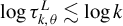 $\log \tau ^{L}_{k,\theta }\lesssim \log k$
.
We apply the sieve score bootstrap (Chen and Christensen, Reference Chen and Christensen2018) to compute critical values so that the UCBs can attain uniform probability coverage over
 $\mathcal {C}$
. In what follows, we introduce the sieve score bootstrap method and prove its uniform size controls for the cases of stationary mixingale and near-unity regressors imposed by Assumptions 2 and 3.
Let
 $\{\omega _{i}\}_{i\in [n]}$
be iid standard Gaussian variates (
 $\omega _{i}\sim \mathcal {N}(0,1)$
) which are independent of data
 $(y_{it},x^{\prime }_{it},\epsilon _{it})^{\prime }$
. Then, we define the sieve score bootstrapping t-statistic process as
 $$ \begin{align} &t^{b}_{\theta}(x):=\frac{l_{\theta}(x)^{\prime}\left(\mathbb{E}_{n}[\mathbb{E}_{T}[\widetilde{p}_{it}\widetilde{p}^{\prime}_{it}]]\right)^{-1}\left\{\mathbb{G}_{n}\left[\omega_{i}\cdot\mathbb{G}_{T}\left[\widetilde{p}_{it}\widehat{\widetilde{\epsilon}}_{it}\right]\right]\right\}}{\widehat{\sigma}_{\theta}(x)}, \end{align} $$
for each
 $x\in \mathcal {C}$
with
 $\widehat {\widetilde {\epsilon }}_{it}$
defined in calculating (24). To compute the critical values
 $cv_{n}^{b}(1-\alpha )$
of UCBs, one calculates
 $\sup _{x\in \mathcal {C}}\vert t^{b}_{\theta }(x)\vert $
based on a large number of iid draws of
 $\{\omega _{i}\}_{i\in [n]}$
which are independent from data. Therefore, the critical value
 $cv_{n}^{b}(1-\alpha )$
can be constructed by the
 $(1-\alpha )$
quantile of
 $\sup _{x\in \mathcal {C}}\vert t^{b}_{\theta }(x)\vert $
over the multiple random draws of the perturbation processes
 $\{\omega _{i}\}_{i\in [n]}$
, as
 $$ \begin{align} cv^{b}_{n}(1-\alpha):=(1-\alpha)\text{ quantile of}~\sup_{x\in\mathcal{C}}\vert t^{b}_{\theta}(x)\vert~\text{given the data and }\{\omega_{i}\}_{i\in[n]}. \end{align} $$
Further, we can develop the UCBs for the linear functional
 $\theta (x)$
by
 $$ \begin{align} \left[\widehat{\theta}^{b}_{l}(x),\widehat{\theta}^{b}_{u}(x)\right]=\left[\widehat{\theta}(x)-cv^{b}_{n}(1-\alpha)\cdot\widehat{\sigma}_{\theta}(x),~\widehat{\theta}(x)+cv^{b}_{n}(1-\alpha)\cdot\widehat{\sigma}_{\theta}(x)\right],~~\text{for}~x\in\mathcal{C}, \end{align} $$
in which
 $cv^{b}_{n}(1-\alpha )$
ensures that
 $\theta (x)\in [\widehat {\theta }^{b}_{l}(x),\widehat {\theta }^{b}_{u}(x)]$
for all
 $x\in \mathcal {C}$
with the asymptotic confidence level
 $100(1-\alpha )\%$
for both the cases of the stationary mixingale and near unit root regressors imposed by Assumptions 2 and 3.
To facilitate the empirical applications of the bootstrapping UCBs for linear functionals, we detail its construction in the following algorithm.
Algorithm 1 (UCBs for Linear Functionals)
-
(i) Step 1: Compute the nonparametric sieve estimator
$\widehat {\theta }(\cdot )$
in Section 4 of the main article; Compute the sample moment and variances,
$\widehat {Q}$
,
$\widehat {\Sigma ,}$
and
$\widehat {\Omega }$
provided in (24). -
(ii) Step 2: Draw the iid standard Gaussian variates
$\{\omega _{i}\}_{i\in [n]}$
which are independent of data
$(y_{it},x^{\prime }_{it},\epsilon _{it})^{\prime }$
and simulate the bootstrap sup-test
$\sup _{x\in \mathcal {C}}\vert t^{b}_{\theta }(x)\vert $
with
$t^{b}_{\theta }(x)$
of (27). -
(iii) Step 3: Repeat Step 2 for B times and calculate the
$(1-\alpha )$
quantile of the sup-test,
$\sup _{x\in \mathcal {C}}\vert t^{b}_{\theta }(x)\vert $
; Report the
$(1-\alpha )$
confidence level two-sided UCB of (29).


The uniform size controls of the proposed UCBs are proved in the following theorem.
Theorem 4.1 (Uniform Inference of Sieve Score Bootstrap)
Suppose that Assumptions 1, 2 (or 3), 4, 5, 6, 7, and 8 and other conditions of Theorem 3.1 hold. Assume that
 $cv^{b}_{n}\left (1-\alpha \right )$
is constructed as in (28). Then, the confidence bands defined in (29) satisfy
 $$ \begin{align} &\Pr\left\{\theta(x)\in\left[\widehat{\theta}^{b}_{l}(x),\widehat{\theta}^{b}_{u}(x)\right],~\text{for all }x\in{\mathcal{C}}\right\}=1-\alpha+o\left(1\right). \end{align} $$
Theorem 4.1 applies the sieve score bootstrap in Chen and Christensen (Reference Chen and Christensen2018) to the fixed-effects nonparametric panel data model that incorporates either the stationary mixingale or near unit root process and proves the validity of our proposed UCBs. In such a case, though the unit root process that can result in nonstandard distributions exists, we can still apply the cross-sectional averaging to retain the Gaussian approximation and prove the uniform probability coverage of the sieve score bootstrap UCBs.
Remark 6. The uniform testing method that involves the unit root process requests a strong approximation theory to the empirical process of the test statistic. However, the sample moment and covariance generated from the nonstationary time series (Phillips, Reference Phillips1987) conventionally call upon the invariance principle and random weak limits, which cannot be compatible with the matrix LLN and coupling principles. To deal with the challenge that arises from the nonstandard limit theory of the unit root process, we use panel data and obtain the standard Gaussian limit theory by focusing on the additional averaging over cross-sectional individuals. That is, we treat the scaled time-series averaging as the generated variables and only count on the high-dimensional CLT over i. In this manner, Yurinskii’s coupling and the matrix LLN can still be applied to the present context.
Accordingly, the sieve score bootstrap method of Chen and Christensen (Reference Chen and Christensen2018) is modified to accommodate the fixed-effects nonparametric panel model of (1). The underlying intuition of the sieve score bootstrap is randomizing the independent component (generated variable) by the perturbation process to recover the uniform null distribution of the test statistic. As mentioned above, the independent generated variable of the current context is the time-series averaging component. So, our proposed bootstrapping method randomizes the time-series averages rather than the unit-specific element for each i and t. Therefore, the article makes another contribution to the literature by showing that the modified sieve score bootstrap method can help attain the uniform probability coverage for the nonparametric exogenous shocks in both the conventional individual fixed-effects panel model and the two-way fixed-effects panel model that is discussed in Section 5.
Remark 7. When the dimension of regressors is large (d is large), the efficiency loss and computational burdens of the nonparametric estimation method increase dramatically. This is the so-called “curse of dimensionality.” In the literature, Stone (Reference Stone1980), which gave the minimax optimal rate of the nonparametric estimator, addressed this issue. We quote their main finding for illustration: Define
 $(X, Y)$
to be iid with
 $X\in \mathbb {R}^d$
valued and Y being scalar. Stone (Reference Stone1980) showed that
 $n^{-s /(2s+d)}$
is the
 $L_2$
minimax optimal rate for estimators of regression functions which rely on a random sample of size n. Here, the quantity s denotes the order of smoothness of regression functions. It is evident that as d (the number of regressors) increases, the optimal rate will be monotonically reduced. This rate shows the negative effects of an increasing number of regressors on the optimal convergence rate. This result also holds for all nonparametric/machine-learning methods and can be intentionally extended to panel data.
One possible solution strategy to resolve this issue is introducing the semi-nonparametric approach, which relies on the partial linear panel model as
 $$ \begin{align} y_{it}={\gamma_{i}}+g(x_{it})+z_{it}^{\prime}\eta+\epsilon_{it},~~\mathbb{E}\left[\epsilon_{it}|x_{it},z_{it}\right]=0, \end{align} $$
in which
 $x_{it}$
is the one-dimensional regressor of interest and
 $z_{it}$
is a d-dimensional control variable. To help improve the estimation efficiency, we put the control variates into the parametric part while investigating the nonlinear effects of the independent variable of interest. We apply the sieve expansion to
 $g(\cdot )$
and obtain the approximate linear model:
 $$ \begin{align} y_{it}=\gamma_{i}+p^{\prime}_{it}\beta+z_{it}^{\prime}\eta+u_{it},~~u_{it}:=r_{it}+\epsilon_{it}. \end{align} $$
Then, we derive the least squares estimators
 $\widehat {\beta }$
and
 $\widehat {\eta }$
and obtain the nonparametric estimator
 $\widehat {g}(\cdot )$
. Further steps for constructing the bootstrapping UCBs follow Algorithm 1, and the uniform size controls can be shown by Theorem 4.1. It is also worth mentioning that the semi-nonparametric bootstrapping UCB for (31) is a special case of the uniform inference procedure in the additive nonparametric panel model given in Section C.ii of the Supplementary Material. Simulation studies examine both the cases of a partial linear functional form and of an additive functional form and show the robustness of our proposed bootstrapping UCBs, which can help attain uniform probability coverage. In addition, the empirical analysis also applies both the methods that rely on the partial linear form and the additive functional form to the real data.
Remark 8. This remark discusses the choice of the tuning parameter k. Our uniform inference procedure relies on uniform asymptotics, with a rate of convergence being derived in terms of the
 $ L_\infty $
norm. Comparatively, the cross-validation criterion approximates the mean squared error (MSE) that balances the squared bias and variance components. This data-driven method works by relying on the
 $L_2$
norm and can be treated as a valid model selection method of tuning parameters in pointwise asymptotics rather than uniform asymptotics. Given this reason, the cross-validation method may not be a suitable candidate for our uniform inference framework.
The uniform convergence rate of our article can be challenging to approximate since the exact approximation error is difficult to evaluate. So, the number of sieve basis functions cannot be directly estimated given this theoretical result. As an alternative, this article uses simulation studies to search for a suitable choice that yields the desirable finite-sample performance. Simulation results show that once the number of basis functions is bigger than
 $6$
, the finite-sample probability coverage of our UCBs can be close to the nominal level. This choice of basis functions will also be applied to our empirical studies, which will be introduced later.
Similarly, the related discussions in Li and Liao (Reference Li and Liao2020) and Li et al. (Reference Li, Liao and Zhou2024) rely on simulation findings to choose the number of basis functions and show the robustness of this choice. So, their results corroborate the feasibility of our rule of selecting tuning parameters.
5 EXTENSIONS TO TWO-WAY FIXED-EFFECTS PANEL MODEL
Econometricians widely apply the two-way fixed-effects panel for estimating causal effects in empirical work, mainly for two reasons: first, by including the fixed effects in both time and cross-sectional dimensions, we can control unobserved confounders and remove endogeneity; second, the two-way fixed-effects panel model reduces to the difference-in-difference panel model under the simplest setting with two groups and two time periods.
This section further extends the uniform inference procedure to the case of the nonparametric panel model with two-way fixed effects:
 $$ \begin{align} y_{it}=\gamma_{i}+f_t+g(x_{it})+\epsilon_{it},~~\mathbb{E}\left[\epsilon_{it}| \{x_{it}\}_{t\in[T]}\right]=0,~~i\in[n]~\text{and}~t\in[T], \end{align} $$
in which
 $x_{it}$
,
 $\epsilon _{it}$
, and
 $\gamma _i$
follow the setup of (1) and
 $f_t$
denotes the time fixed effect that is correlated with regressor
 $x_{it}$
. Different from the setup of the model that only includes the individual fixed effects, we allow for a large panel in which both n and T diverge.
Based on the sieve expansion, we similarly obtain a linear panel data model as
 $$ \begin{align} y_{it}=\gamma_{i}+f_t+p^{\prime}_{it}\beta+u_{it},~~u_{it}:=r_{it}+\epsilon_{it}. \end{align} $$
With a slight abuse of notation, we define a new approach of demeaning as
 $$ \begin{align} &\widetilde{y}_{it}:=y_{it}-\mathbb{E}^{\ast}_T[y_{is}]-\mathbb{E}_n[y_{is}]+\mathbb{E}_n[\mathbb{E}_T^{\ast}[y_{is}]], \end{align} $$
 $$ \begin{align} &\widetilde{p}_{it}:=p_{it}-\mathbb{E}_T^{\ast}[p_{is}]-\mathbb{E}_n[p_{is}]+\mathbb{E}_n[\mathbb{E}_T^{\ast}[p_{is}]], \end{align} $$
 $$ \begin{align} &\widetilde{u}_{it}:=y_{it}-\mathbb{E}_T^{\ast}[u_{is}]-\mathbb{E}_n[u_{is}]+\mathbb{E}_n[\mathbb{E}_T^{\ast}[u_{is}]]. \end{align} $$
Then, we follow the identification condition of Assumption 4 and compute the least squares estimate
 $\widehat {\beta }$
of (10) and the nonparametric estimator
 $\widehat {g}(\cdot )$
of (11) by using the demeaned variates
 $\widetilde {y}_{it}$
,
 $\widetilde {x}_{it}$
, and
 $\widetilde {\epsilon }_{it}$
defined in (35)–(37). To construct the UCBs for linear functionals
 $\theta (x)$
of
 $g(x)$
, we also compute the sample moment and variance estimates
 $\widehat {Q}$
,
 $\widehat {\Sigma }$
, and
 $\widehat {\Omega }$
based on
 $\widetilde {y}_{it}$
and
 $\widetilde {x}_{it}$
of (35) and (36) and the residual estimate
 $\widehat {\widetilde {\epsilon }}_{it}:=\widetilde {y}_{it}-\widetilde {p}^{\prime }_{it}\widehat {\beta }$
. Then, we can attain the variance estimate
 $\widehat {\sigma }^2_{\theta }(x)$
based on (25). To implement the sieve score bootstrap method, we calculate the simulated empirical process of (27) and take
 $cv^{b}_{n}(1-\alpha )$
in (28) to build the UCBs with the
 $100(1-\alpha )$
% confidence level
 $$ \begin{align} \left[\widehat{\theta}^{b}_{l}(x),\widehat{\theta}^{b}_{u}(x)\right]=\left[\widehat{\theta}(x)-cv^{b}_{n}(1-\alpha)\cdot\widehat{\sigma}_{\theta}(x),~\widehat{\theta}(x)+cv^{b}_{n}(1-\alpha)\cdot\widehat{\sigma}_{\theta}(x)\right], \end{align} $$
for any compact subset
 $\mathcal {C}\subseteq \mathcal {X}$
. The computational procedure follows the details in Algorithm 1 of Section 4.
Similar to Theorem 4.1, we prove the uniform size control of the UCBs given by (38) in the following theorem.
Theorem 5.1 (Uniform Inference of Sieve Score Bootstrap)
Suppose that Assumptions 1, 2, and 4–8 and other conditions of Theorem 3.1 hold. Then,
 $$ \begin{align*} \Pr\left\{\theta(x)\in\left[\widehat{\theta}^{b}_{l}(x),\widehat{\theta}^{b}_{u}(x)\right],~\text{for all }x\in{\mathcal{C}}\right\}=1-\alpha+o(1). \end{align*} $$
It is worth mentioning that the time fixed effect
 $f_t$
allows for various types of persistence, including not only the stationary mixingale, mildly stationary, unit root, and local-to-unity processes but also the deterministic trends, while the regressor
 $\{x_{it}\}$
follows the stationary mixingale condition of Assumption 2. The robustness of our inference method enables the broad applicability of our framework in a wide class of panel models.
Though the time effect,
 $f_t$
, introduces cross-sectional dependence, Theorem 5.1 utilizes the independence of the population moments that involve
 $f_t$
in the score vector to motivate Yurinskii’s coupling principle and uniform inference. More detailed discussions and proofs given in the Supplementary Material will be omitted in the main article for simplicity. Extensive simulation studies that examine the finite-sample performance of the UCBs in the two-way fixed-effects panel model (33) are also collected in the Supplementary Material.
6 MONTE CARLO SIMULATIONS
This section evaluates the finite sample performance of our bootstrapping UCBs and pointwise CIs that use the Gaussian critical values. Namely, we consider four types of models, including the one-way and two-way fixed-effects panel models with a univariate regressor (Models 1 and 3; Equations (1) and (33)), the one-way fixed-effects partial linear panel model with multivariate regressors (Model 2-1; Equation (31)), and the one-way fixed-effects panel data model with an additive functional form (Model 2-2; Equation (C.5) of the Supplementary Material).
6.1 Simulation Setup
The simulations reported below involve four models (Model 1, Model 2-1, Model 2-2, and Model 3) which are designed as follows.
For the univariate model with one-way fixed effects (Model 1), to ensure the intertemporal correlations for regressors and also the correlation between fixed effect and regressors, we set the regressor
 $x_{it}=\phi _{x} x_{i,t-1}+v^{\ast }_{it}$
and the fixed effects
 $\gamma _{i}=(1/T)\sum _{t=1}^T \Phi \left (w^{\ast }_{it}\right )$
, in which the function
 $\Phi $
is the Gaussian CDF and
 $\left (w^{\ast }_{it}, v^{\ast }_{it}\right )$
are iid draws from a joint normal distribution with zero means, unity variances, and covariance terms
 $\mathbb {E}[w^{\ast }_{it}v^{\ast }_{it}]=0.5$
. The term
 $\{u_{\epsilon ,it}\}$
is randomly drawn from
 $\mathcal {N}(0,1)$
that is independent of
 $(w^{\ast }_{it},v^{\ast }_{it})^{\prime }$
and the
 $\{\epsilon _{it}\}$
follows
 $\epsilon _{it}=\phi _{\epsilon }\epsilon _{i,t-1}+u_{\epsilon ,it}$
. The autoregressive slope
 $\phi _{x}\in \{0.5,1-1/T^{0.5},0.92,1,1.03\}$
and
 $\phi _{\epsilon }=0.2$
. It is evident that our DGPs cover the cases of stationary (
 $\phi _x=0.5$
), mildly stationary (
 $\phi _x=1-1/T^{0.5}$
), and unity/local-to-unity (
 $\phi _x=1$
), staying consistent with the theoretical derivations. In addition, parts of the simulated autoregressive roots are taken from empirical estimates in the next section; for instance, the estimated roots,
 $0.9217$
and
 $1.0317$
, are captured from the dynamics of asset holding and income.
For the multivariate panel data model with one-way fixed effects (Models 2-1 and 2-2), we use the bivariate regressors
 $x_{1,it}=\phi _{x1} x_{1,i,t-1}+v^{\ast }_{1,it}$
,
 $x_{2,it}=\phi _{x2} x_{2,i,t-1}+v^{\ast }_{2,it}$
and the individual fixed effects
 $\gamma _{i}=(1/T)\sum _{t=1}^T \Phi \left (w^{\ast }_{it}\right )$
, in which the function
 $\Phi (\cdot )$
is the Gaussian CDF and
 $(w^{\ast }_{it}, v^{\ast }_{1,it}, v^{\ast }_{2,it})$
are iid draws from the joint Gaussian distribution with zero means, unity variances, and covariance terms
 $\mathbb {E}[w^{\ast }_{it}v^{\ast }_{1,it}]=\mathbb {E}[w^{\ast }_{it}v^{\ast }_{2,it}]=0.5$
and
 $\mathbb {E}[v^{\ast }_{1,it}v^{\ast }_{2,it}]=0.25$
. The error term
 $\epsilon _{it}$
is identical to the univariate panel in Model 1. The autoregressive coefficients are set as
 $\phi _{x1},\phi _{x2}\in \{0.5,0.92, 1,1.03\}$
, in which the autoregressive roots
 $\phi _{x1},\phi _{x2}\in \{0.92, 1.03\}$
are estimated from empirical analysis.
In the univariate panel model with two-way fixed effects (Model 3), we set the regressor
 $x_{it}=\phi _{x} x_{i,t-1}+v^{\ast }_{it}$
, the individual fixed effects
 $\gamma _{i}=(1/T)\sum _{t=1}^T \Phi \left (w^{\ast }_{1,it}\right )$
, and the time fixed effects
 $f_t=\phi _{f}f_{t-1}+w_{2t}^{\ast }$
with
 $w_{2t}^{\ast }=(1/n)\sum _{i=1}^n w^{\ast }_{2,it}$
, in which the function
 $\Phi (\cdot )$
is the Gaussian CDF and
 $\left (w^{\ast }_{1,it}, w^{\ast }_{2,it}, v^{\ast }_{it}\right )$
are iid draws from the joint Gaussian distribution with zero means, unity variances, and the covariances
 $\mathbb {E}[w^{\ast }_{1,it}v^{\ast }_{it}]=\mathbb {E}[w^{\ast }_{2,it}v^{\ast }_{it}]=0.5$
and
 $\mathbb {E}[w^{\ast }_{1,it}w^{\ast }_{2,it}]=0$
. The error
 $\epsilon _{it}$
is set identically as the univariate panel model with one-way fixed effects. The autoregressive parameters
 $\phi _{x}\in \{0.5,0.92\}$
and
 $\phi _{f}=0.5$
.
We conduct simulation studies with functional forms given by
 $$ \begin{align} \text{F1:}~&g(x)=\sin(x)\exp(-x^2/2), \end{align} $$
 $$ \begin{align} \text{F2:}~&g(x_1,x_2)=\sin(x_1)\exp(-x_1^2/2)+x_2, \end{align} $$
 $$ \begin{align} \text{F3:}~&g(x_1,x_2)=\sin(x_1)\exp(-x_1^2/2)+x_2\exp(-x_2^2/2). \end{align} $$
To be specific, the functional form F1 is applied to the univariate models, Models 1&3, and the forms F2 and F3 correspond to the multivariate models with partial linear form (Model 2-1) and additive functional form (Model 2-2).
We generate
 $10{,}000$
simulation paths with the schemes of sample size
 $\{n=100,T=500\}$
and
 $\{n=792,T=6\}$
for each model.Footnote
6
For each simulated path, we implement our method using the Hermite basis functions to approximate the unknown functional, the first-order partial derivative regarding the entry of interest (
 $\partial g(\cdot )$
for F1 and
 $\partial _{x_1}g(\cdot ,\cdot )$
for F2 and F3). Also, we use different values for the order of Hermite sieve expansions, k (
 $k\in \{6,7,8\}$
), to check the robustness of simulation performance. We choose the bandwidth for the HAC estimation by using
 $\lfloor T^{1/3}\rfloor $
when
 $T\geq 10$
and use the conventional simple variance estimator when
 $T<10$
.
In this simulation study, we care about the shape of
 $g(\cdot )$
, particularly the first-order partial derivative,
 $\partial g(\cdot )$
(or
 $\partial _{x_1} g(\cdot )$
). For each experiment, we calculate the
 $90$
%,
 $95$
%, and
 $99$
% UCBs for
 $\partial g(\cdot )$
(or
 $\partial _{x_1} g(\cdot )$
) over the chosen set
 $[\underline {x}, \overline {x}]$
Footnote
7
with
 $1{,}000$
bootstrap replications. To implement the uniform inference methods, we randomly draw the bootstrap innovations
 $\omega _i$
from the standard normal distribution to construct the critical values of sup-test. We then calculate the probability coverage of our bootstrapping UCBs of interestFootnote
8
and compare it with that of the pointwise CIs based on the Gaussian critical values.
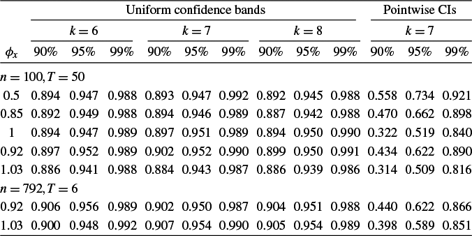
The details of the bootstrapping UCBs for the one-way fixed-effects univariate panel model are presented in Table 1, giving the empirical probability coverage under the uniform null hypothesis. By comparing the estimated probability coverage levels with their nominal values (
 $90$
%,
 $95$
%, and
 $99$
%), we can find that the UCBs attain the nominal level, illustrating that the sup-type statistics can control over-rejections nicely across all
 $x\in \mathcal {C}$
and with stationary/mildly stationary/local-to-unity regressors. Comparatively, the pointwise CIs attain severe size distortions at all significance levels, again demonstrating the risk of spurious statistical significance.
Probability coverage (PC) of uniform and pointwise confidence bands for one-way fixed-effects univariate panel models (Model 1) with the function form (F1)

Note: aThe
 $\phi _x$
values
 $0.5$
,
 $0.85(=1-1/50^{0.5})$
and
 $1$
denote stationary, mildly stationary, and unity roots. bThe
 $\phi _x$
values
 $0.92$
and
 $1.03$
are estimated from the empirical data of asset holding and income. cThe simulated size
 $n=792,~T=6$
mimics the sample size of empirical data. dThe kth-order Hermite basis expansion applies to the nonparametric component (
 $k=6,7,8$
). eThe uniform and pointwise confidence bands are computed for
 $\partial _{x} g(\cdot )$
.
Further sensitivity analysis for the choice of sieve expansion order, k, is given in Table 1, in which we examine the order of Hermite basis expansions, namely,
 $k=6$
,
 $7$
, and
 $8$
. Our bootstrapping UCBs show satisfying size controls across these cases, so it is reasonable to apply these choices of k to empirical analysis. Among these choices, it is well evident that the bootstrapping UCBs with
 $k=7$
demonstrate the empirical rejection rates closest to the nominal levels. By this observation, we use the tuning parameter
 $k=7$
in our empirical analysis of the next section.
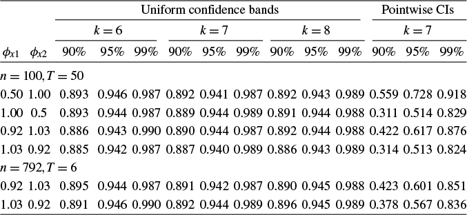
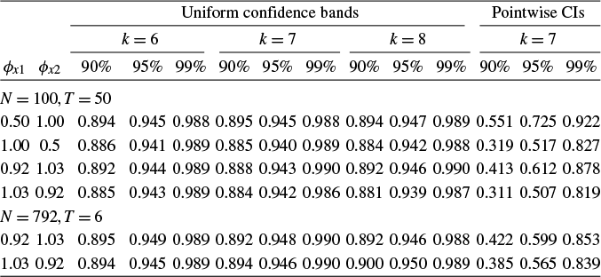
Simulation results for the one-way fixed-effects multivariate model with the partial linear form are in Table 2, providing the empirical sizes of our bootstrapping UCBs and pointwise CIs. Overall, all these simulations show that the sieve score bootstrapping method provides uniform probability coverage for the partial linear panel model in finite samples, corroborating that the bootstrapping UCBs can help reduce spurious significance regarding the uniform null hypothesis robustly. This robust performance holds across nonstationary regressors and various choices of tuning parameter k. It is well evident that the empirical size performance in the partial linear panel model is best controlled around the nominal level when
 $k=7$
, which is suggested for our empirical study. Similar patterns can also be found in the bivariate panel data models with additive functional forms, as presented in Table 3.
Probability coverage (PC) of uniform and pointwise confidence bands for one-way fixed-effects multivariate panel models (Model 2-1) with a partial linear form (F2)

Note: aThe kth-order Hermite basis expansion applies to the nonparametric component of
 $x_1$
(
 $k=6,7,8$
). bThe uniform and pointwise confidence bands are computed for
 $\partial _{x_1} g(\cdot ,\cdot )$
.
Probability coverage (PC) of uniform and pointwise confidence bands for one-way fixed-effects multivariate panel models (Model 2-2) with an additive function form (F3)

Note: aThe kth-order Hermite basis expansion applies to the nonparametric component of both
 $x_1$
and
 $x_2$
(
 $k=6,7,8$
). bThe uniform and pointwise confidence bands are computed for
 $\partial _{x_1} g(\cdot ,\cdot )$
.
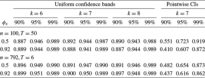
Table 4 gives the empirical size behaviors of our UCBs in the two-way fixed-effects panel data model. With stationary regressors, the probability coverage of UCBs is very close to the nominal level, showing the flexibility of our method in allowing for the two-way fixed-effects panel model. Furthermore, when an autoregressive root close to unity (e.g.,
 $0.92$
) is included in the simulation study, the degree of robustness is well shown; for instance, when across all levels of significance, the empirical size performances of UCBs are well controlled. In comparison, the pointwise CIs that use the Gaussian critical values encounter severe size distortions in specifying the uniform null hypothesis. Similarly, by evaluating the behaviors of different k, we find that the choice of
 $k=7$
helps attain the best-controlled size performance.
Probability coverage (PC) of uniform and pointwise confidence bands for two-way fixed-effects panel models with the function form (F1)

Note: aThe kth-order Hermite basis expansion applies to the nonparametric component of x (
 $k=6,7,8$
). bThe uniform and pointwise confidence bands are computed for
 $\partial g(\cdot )$
.
7 EMPIRICAL ILLUSTRATION
In this section, we use the data of the Panel Survey of Income Dynamics (PSID) from 1999 to 2009 (six waves) to examine the influence of financial status on consumption. We estimate consumption responses to income and asset holdings and establish the UCBs to investigate the nonlinear relationships.
Similar to Arellano, Blundell, and Bonhomme (Reference Arellano, Blundell and Bonhomme2017), we proceed to estimate a model that allows for nonstationary measures of assets in a sample of homogeneous households from the PSID data. For instance, the households hold a one-period bond whose return
 $\{a_{it}\}$
follows a nonstationary relationship with an autoregressive root
 $(1+r)>1$
as
 $$ \begin{align} a_{i,t+1}=\left(1+r\right)a_{it}+i_{it}-c_{it}, \end{align} $$
in which
 $a_{it}$
,
 $i_{it}$
, and
 $c_{it}$
denote the asset, disposable income, and consumption, respectively. Since
 $a_{it}$
follows a nonstationary process whose root is close to unity, it is worth mentioning that our uniform inference procedures can naturally allow for nonstationary regressors of the unit root type.
The baseline model in our discussion is formulated as
 $$ \begin{align} c_{it}=\gamma_{i}+g\left(a_{it},i_{it}\right)+\epsilon_{it}, \end{align} $$
in which
 $c_{it}$
is the consumption of households and the covariates
 $a_{it}$
and
 $i_{it}$
denote the asset and income. By applying the within-group sieve estimator that relies on the Hermite basis functions, we intend to find the presence of nonlinear impacts of assets and income on the consumption of households.
To give the UCBs for functionals
 $\partial _{a} g(\cdot ,\cdot )$
and
 $\partial _{i} g(\cdot ,\cdot )$
, we discuss two types of specifications for its functional form: the partial linear form and the additive functional form:
 $$ \begin{align*} &\text{(i)}~g(a_{it},i_{it})=m(i_{it})+\eta_1 a_{it};~\text{(ii)}~g(a_{it},i_{it})=m(a_{it})+\eta_2 i_{it};\\& \quad \text{and (iii)}~g(a_{it},i_{it})=m_1(a_{it})+m_2(i_{it}). \end{align*} $$
We utilize these specifications and discuss their UCBs. Computations and asymptotics of the sieve score bootstrapping UCBs for the partial linear model and the additive functional form are given in Remark 7 of the main article and Section C.ii of the Supplementary Material.


The sieve expansion order
 $k=7$
for both these models, as suggested by simulation studies. Based on (24), we apply the variance estimator that is designed for the case of a small T, since
 $T=6$
. The sup-type statistics to test for nonlinear patterns are computed on the
 $200$
evenly chosen grid points between
 $20\%$
and
 $80\%$
quantiles of the variable of interest. Figures 1(a) and 1(c) show the nonlinear dynamics of consumption concerning income shocks and show the results for both the partial linear and additive functional forms. It is worth mentioning that the
 $95\%$
pointwise CIs show that households tend to increase consumption when positive changes are expected for nearly all levels. In comparison, it is evident that the
 $95\%$
UCBs have larger widths and reveal that only positive changes that occur for the income of a higher level will increase consumption. Also, it is shown that the approaches for the additive and the partial linear functional forms produce similar empirical findings.
Figures 1(b) and 1(d) discuss the dynamics of consumption concerning asset holdings and show the empirical results that rely on the partial linear and additive functional forms. Our bootstrapping UCBs show that the nonlinear dynamics in the consumption concerning asset holdings are statistically significant on the
 $5\%$
level. Also, it is revealed that the UCBs have wider widths than the pointwise confidence intervals that use the Gaussian critical values. The UCBs that depend on both types of panel models show similar patterns, demonstrating the robustness of our findings.
8 CONCLUSION
We develop uniform inference procedures for the nonparametric/semi-nonparametric panel models with fixed effects. In the framework of the present article, we allow for general forms of intertemporal correlations in regressors, including stationary mixingale, mildly stationary, or local-to-unity process. We extend this uniform inference method to the nonparametric panel model with two-way fixed effects. While the pointwise inference problem of the nonparametric panel models has been extensively explored in the literature, the sup-type test statistic has not been discussed in the literature. The present article contributes significantly to this area by filling the void.
To the best of our knowledge, our work makes the first attempt to consider the uniform inference procedure (sup-test) in the nonparametric panel model with individual fixed effects. Further extension of our framework can consider cross-sectional correlations represented as interactive fixed-effect models or social interaction models. Such discussions are beyond the scope of the present article and will be left for our future research.
COMPETING INTEREST STATEMENT
The authors declare no competing interests exist.
FUNDING STATEMENT
Yanbo Liu acknowledges that this project is supported by the National Natural Science Foundation of China (NSFC) under Grant No. 72303130. Nan Liu acknowledges that this project is supported by the National Natural Science Foundation of China (NSFC) under Grant No. 72103172.
SUPPLEMENTARY MATERIAL
Liu, N., & Liu, Y. (2025): Supplement to “Uniform Inference for Nonparametric Panel Models with Fixed Effects,” Econometric Theory Supplementary Material. To view, please visit https://doi.org/10.1017/S026646662510025X.
A PROOFS
A.1 Proof of Theorem 3.1
In order to apply the coupling method, we enhance the probability space in which the standard Gaussian variate
 $\mathcal {N}_{k}$
is measurable and apply Yurinskii’s coupling principle (Lemma A.2 of the Supplementary Material) to the empirical process:
 $$ \begin{align*} \frac{1}{\sqrt{n}}\sum^{n}_{i=1}\xi_{i},~~~\xi_{i}:=\Sigma^{-1/2}\mathbb{G}_{T}\left[{\widetilde{p}_{it}}\left(\epsilon_{it}+r_{it}\right)\right]. \end{align*} $$
By definition, it follows that
 $\mathbb {E}[\xi _i]=\mathbf {0}_{k\times 1}$
for each individual i. Another sufficient condition to verify the validity of Yurinskii’s coupling is given as
 $$ \begin{align*} \mathbb{E}\left\Vert \xi_{i}\right\Vert{}^3&\lesssim\mathbb{E}\left\Vert\mathbb{G}_{T}\left[{\widetilde{p}_{it}}\left(\epsilon_{it}+r_{it}\right)\right]\right\Vert{}^3\\ & \lesssim\mathbb{E}\left\Vert\mathbb{G}_{T}\left[{\widetilde{p}_{it}}\right]\right\Vert{}^2{a_{T}}\tau_{k}\left(1+\ell^{3}_{k}c^{3}_{k}\right)\\ &\lesssim k\cdot{a_{T}^3}\tau_{k}\left(1+\ell^{3}_{k}c^{3}_{k}\right), \end{align*} $$
in which we use the facts
 $\sup _{x\in \mathcal {X}}\mathbb {E}\left [\left \vert \epsilon _{it}\right \vert {}^3 \vert x_{it}=x\right ]\lesssim 1$
and
 $\max _{i\in [n]}\max _{t\in [T]}\vert r_{it}\vert \leq \sup _{x\in \mathcal {X}}\left \vert r_g(x)\right \vert \lesssim \ell _{k}c_k$
. The strong approximation in Lemma A.2 of the Supplementary Material yields that
 $$ \begin{align} \Pr\left\{\left\Vert \frac{\sum^{n}_{i=1}\xi_{i}}{\sqrt{n}}-\mathcal{N}_{k}\right\Vert\geq 3\delta c^{-1}_{nT}\right\}&\lesssim\frac{k^{2}a^3_{T}\tau_{k}\left(1+\ell_{k}^{3}c^{3}_{k}\right)}{\left(\delta c^{-1}_{nT}\right)^3\sqrt{n}}\nonumber\\&\quad\left(1+\frac{\log \left(k^2\cdot a_{T}\tau_{k}\left(1+\ell^{3}_{k}c^{3}_{k}\right)\right)}{k}\right)\rightarrow0, \end{align} $$
due to the rate restriction that
 $c^{6}_{nT}k^4a^{6}_{T}\tau ^{2}_{k}(\log n)^2/n\rightarrow 0$
.
Based on the linear approximation of (12), we obtain the following:
 $$ \begin{align} &\left\Vert \sqrt{n}{a_{T}\cdot}\alpha(x)^{\prime}\left(\widehat{\beta}-\beta\right)-\alpha(x)^{\prime}\Omega^{1/2}\mathcal{N}_{k}\right\Vert \notag \\ &\quad\leq \left\Vert \mathbb{G}_n[\alpha(x)^{\prime}\Omega^{1/2}\xi_{i}]-\alpha(x)^{\prime}\Omega^{1/2}\mathcal{N}_{k}\right\Vert+\overline{R}_{1,nT}+\overline{R}_{2,nT}=o_{p}\left(c^{-1}_{nT}\right), \end{align} $$
over
 $x\in \mathcal {C}$
, by the stochastic boundedness of
 $\Vert \alpha (x)^{\prime }\Omega ^{1/2}\Vert $
, Proposition A.1 of the Supplementary Material, (A.1) and the conditions imposed for
 $\overline {R}_{1,nT}$
and
 $\overline {R}_{2,nT}$
in Theorem 3.1. Therefore, under the condition
 $\sup _{x\in \mathcal {X}}n^{1/2} a_{T}\vert r_{g}(x)\vert /\Vert s(x)\Vert =o_p\left (c^{-1}_{nT}\right )$
, equation (19) holds.
A.2 Proof of Theorem 4.1
By Proposition A.1 of the Supplementary Material, it follows that
 $$ \begin{align} \left\vert\frac{\widehat{\sigma}_{\theta}(x)}{\sigma_{\theta}(x)}-1\right\vert\lesssim_{p}{M\cdot}\left(v_{nT}\vee 1+\ell_{k}c_{k}\right)\left(\sqrt{\frac{\xi^{2}_{k}\log k}{n}}+\frac{1}{k}\right)=o(c^{-1}_{nT}), \end{align} $$
uniformly over
 $x\in \mathcal {C}$
, ensured by the imposed conditions. Similar to Theorem 3.1,
 $$ \begin{align} \frac{\widehat{\theta}(x)-\theta(x)}{ \sigma_{\theta}(x)}=\sqrt{n}{a_{T}\cdot}\frac{\widehat{\theta}\left(x\right)-\theta\left(x\right)}{\left\Vert l_{\theta}\left(x\right)^{\prime}\Omega^{1/2}\right\Vert}=\frac{l_{\theta}\left(x\right)^{\prime}\Omega^{1/2}}{\left\Vert l_{\theta}\left(x\right)^{\prime}\Omega^{1/2}\right\Vert}\mathcal{N}_{k}+o_{p}\left(c^{-1}_{nT}\right),~~\text{in}~L_{\infty}\left(\mathcal{C}\right). \end{align} $$
Combining (A.3) and (A.4), we can further show that
 $$ \begin{align} t_{\theta}(x)=\frac{\widehat{\theta}(x)-\theta(x)}{ \widehat{\sigma}_{\theta}(x)}=\frac{l_{\theta}\left(x\right)^{\prime}\Omega^{1/2}}{\left\Vert l_{\theta}\left(x\right)^{\prime}\Omega^{1/2}\right\Vert}\mathcal{N}_{k}+o_{p}\left(c^{-1}_{nT}\right),~~\text{in}~L_{\infty}\left(\mathcal{C}\right). \end{align} $$
Next, we proceed to show the validity of our sieve score bootstrap method for attaining uniform size controls. We employ Yurinskii’s coupling principle (Lemma A.2 of the Supplementary Material). To apply the strong approximation, we enhance the probability space in which the standard Gaussian variate
 $\mathcal {N}_{k}$
is measurable and apply the coupling principle to
 $$ \begin{align} \frac{1}{\sqrt{n}}\sum^{n}_{i=1}\xi^{\ast}_{i},~~~\xi^{\ast}_{i}:=\Sigma^{-1/2}\omega_{i}\cdot\mathbb{G}_{T}\left[{\widetilde{p}_{it}}{\widetilde{\epsilon}}_{it}\right]. \end{align} $$
In (A.6), each component as
 $(1/\sqrt {n})\omega _{i}\Sigma ^{-1/2}\cdot \mathbb {G}_{T}[\widetilde {p}_{it}{\widetilde {\epsilon }}_{it}]$
is centered at zero because
 $$ \begin{align*} \mathbb{E}\left[\omega_{i}|\left\{y_{it},x_{it},\epsilon_{it}\right\}_{i\in\left[n\right],t\in\left[T\right]}\right]=0,~\text{for any}~i\in\left[n\right], \end{align*} $$
by the independence between
 $\omega _{i}$
and other random variates. Then, it follows that
 $\mathbb {E}[\xi ^{\ast }_{i}]=\mathbf {0}_{k\times 1}$
for each
 $i\in [n]$
. Next, we verify the sufficient condition for the Gaussian coupling as
 $$ \begin{align*} \mathbb{E}\left\Vert \xi^{\ast}_{i}\right\Vert{}^3&\lesssim\mathbb{E}\left\Vert\omega_{i}\mathbb{G}_{T}\left[{\widetilde{p}_{it}}{\widetilde{\epsilon}}_{it}\right]\right\Vert{}^3 \lesssim\mathbb{E}\left\Vert\mathbb{G}_{T}\left[{\widetilde{p}_{it}}\right]\right\Vert{}^2{a_{T}}\tau_{k}\ \lesssim k\cdot{a^3_{T}}\tau_{k}, \end{align*} $$
in which the conditions
 $\sup _{x\in \mathcal {X}}\mathbb {E}[\vert \epsilon _{it}\vert ^3|x_{it}=x]\lesssim 1$
,
 $\sup _{x\in \mathcal {X}}\vert r_{\theta }(x)\vert \lesssim 1,$
and
 $$ \begin{align*} \sup_{i\in\left[n\right]}\sup_{t\in\left[T\right]}\mathbb{E}\left[\omega^{3}_{i}|\left\{y_{is},x_{is},\epsilon_{is}\right\}_{i\in\left[n\right],s\in\left[T\right]}\right]\lesssim1. \end{align*} $$
Therefore, the coupling of Lemma A.2 of the Supplementary Material yields that for any
 $\delta>0$
,
 $$ \begin{align*} &\Pr\left\{\left\Vert \frac{\sum^{n}_{i=1}\xi^{\ast}_{i}}{\sqrt{n}}-\mathcal{N}_{k}\right\Vert\geq 3\delta c^{-1}_{nT}\right\} \lesssim\frac{nk^{2}a_{T}\tau_{k}}{\left(\delta c^{-1}_{nT}\sqrt{n}\right)^3}\left(1+\frac{\vert \log \left(k^2\cdot a_{T}\tau_{k}\right)\vert}{k}\right)\rightarrow0, \end{align*} $$
due to
 $c^{6}_{nT}k^4a^{6}_{T}\tau ^{2}_{k}\log ^2n/n\rightarrow 0$
. Then, we have
 $$ \begin{align} \sup_{x\in\mathcal{C}}\left\vert t^{b}_{\theta}(x)-\frac{l_{\theta}(x)^{\prime}\cdot \Omega^{1/2}\mathcal{N}_{k}}{\sigma_{\theta}(x)}\right\vert=o(c^{-1}_{nT}). \end{align} $$
Further, combining (A.6) and (A.7), we have
 $$ \begin{align} \sup_{x\in\mathcal{C}}\left\vert t_\theta(x)-t^{b}_{\theta}(x)\right\vert=o(c^{-1}_{nT}), \end{align} $$
in which the t test statistic process is given in (26).
Based on (A.8) and Theorem 5.5 of Belloni et al. (Reference Belloni, Chernozhukov, Chetverikov and Kato2015), it follows that
 $$ \begin{align} \sup_{s\in\mathbb{R}}\left\vert \Pr\left(\sup_{x\in\mathcal{C}}\left\vert t^{b}_{\theta}(x)\right\vert\leq s\right)-\Pr\left(\sup_{x\in\mathcal{C}}\left\vert t_\theta(x)\right\vert\leq s\right)\right\vert=o(1), \end{align} $$
for any
 $s\in \mathbb {R}$
when
 $n\rightarrow \infty $
. In the end, we prove the final result.