

Introduction
Red rice is an annual Oryza sativa characterized by features, such as seed dormancy and shattering, which make it a troublesome weed, infesting rice paddies in temperate areas. In the laboratory, red rice dormancy is overcome by dry-afterripening for 4–8 weeks at ambient temperatures (Cohn and Hughes, Reference Cohn and Hughes1981); the rate and extent of laboratory dry-afterripening are functions of storage temperature and grain moisture content (Cohn and Hughes, Reference Cohn and Hughes1981; Leopold et al., Reference Leopold, Glenister and Cohn1988; Foley, Reference Foley1994). The known afterripening patterns of red rice are generally consistent with the hydrothermal afterripening time model for Bromus tectorum (Christensen et al., Reference Christensen, Meyer and Allen1996; Bair et al., Reference Bair, Meyer and Allen2006). However, the environmental parameters that control red rice germination and dormancy in a field setting have not been characterized.
Various models have been developed to describe and predict seed germination behaviour under both field and laboratory conditions (for a review see Baskin and Baskin, Reference Baskin and Baskin1998). Among these, a model to describe the relationship between germination and temperature/water potential (Gummerson, Reference Gummerson1986) has been subsequently elaborated (Bradford, Reference Bradford1990, Reference Bradford2002), and the hydrotime component of the model has been proposed as an independent tool to describe seed dormancy (Bradford, Reference Bradford and Lang1996). Although some assumptions of hydrothermal time models have been criticized, and interactions between temperature and water potential have been suggested to require more complex analyses (Kebreab and Murdoch, Reference Kebreab and Murdoch1999b), the value of the hydrotime concept has been confirmed (Bradford, Reference Bradford, Kigel and Galili1995; Christensen et al., Reference Christensen, Meyer and Allen1996; Bauer et al., Reference Bauer, Meyer and Allen1998; Kebreab and Murdoch, Reference Kebreab and Murdoch1999b; Finch-Savage and Leubner-Metzger, Reference Finch-Savage and Leubner-Metzger2006; Allen et al., Reference Allen, Benech-Arnold, Batlla, Bradford, Bradford and Nonogaki2007).
Studies of red rice seed survival imply roles for both dormancy cycling in the field (Teekachunhatean, Reference Teekachunhatean1985) and dry-afterripening (Cohn and Hughes, Reference Cohn and Hughes1981) in its germination patterns. Therefore, we characterized the interaction between the effects of the degree of dry-afterripening and the water potential of the incubation medium upon germination, and evaluated the application of a population-based hydrotime model (Bradford, Reference Bradford and Lang1996) to describe the results.
Materials and methods
Seed preparation and incubation
Strawhulled red rice was harvested in 1996 (SH96) and 1998 (SH98) at the LSU Agricultural Center Rice Research Station in Crowley, Louisiana, USA. Mature florets were obtained by hand-shattering of individual plants and were dried in open trays at room temperature (22 ± 2°C) for 4 d. SH96 was stored at − 18°C in sealed glass Mason™ jars until the start of experiments, while SH98 was kept at room temperature (22 ± 2°C) in a sealed glass Mason™ jar for 8 months and considered fully afterripened, using 100% germination as the criterion. Samples of SH96 florets (red rice dispersal units are caryopses enclosed in the hull) were dry-afterripened at 30°C for 1, 2, 3, 4, 6 and 8 weeks. Seed moisture contents at the start of experiments were 11 and 13% for SH96 and SH98, respectively (fresh weight basis). Experiments for 2 and 3 weeks of afterripening were independently repeated twice.
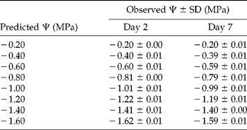
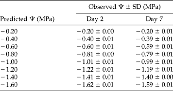
Each sample set was used for two sequential incubation treatments. During the first treatment, intact florets were incubated for 2 weeks at 30°C in polyethylene glycol solutions [PEG; average MW 8000, SigmaUltra (P-4463), Sigma Chemical Co., St. Louis, Missouri, USA] at nine different water potentials (Ψ = 0, − 0.2, − 0.4, − 0.6, − 0.8, − 1.0, − 1.2, − 1.4 and − 1.6 MPa), prepared according to Equation 4 of Michel (Reference Michel1983). Germination was performed in square (9 × 9 cm) plastic Petri dishes, maintained in humidity boxes. Twenty grains were placed in each plate on two sheets of brown germination paper (Anchor Paper Co., St. Paul, Minnesota, USA; the average weight of the paper was 0.89 ± 0.02 g) with 13 ml of PEG; this volume is greater than we have used in our standard germination tests, but was utilized to obtain a solution volume/paper weight ratio of 14.6, i.e. above the threshold indicated by Emmerich and Hardegree (Reference Emmerich and Hardegree1991), to avoid concentration of PEG due to evaporation and filter paper exclusion. Four replicates were used for each Ψ and afterripening time combination. Humidity boxes were kept wrapped with aluminium foil, and all manipulations were performed under a dim green safelight. Germination counts were performed on days 1–7, 9, 11 and 14 (on days 1–7, 9, 11 and 16 for the fully afterripened SH98 sample). Florets were transferred to new Petri dishes containing fresh PEG solutions on days 2, 4 and 7. The solution water potential was measured from each plate on days 4 and 7 (on days 0, 2, 4, 7 and 16 for the experiment with SH98), after seed removal, with a vapour pressure osmometer (Model 5100B, Wescor Inc., Logan, Utah, USA), employing a disc of germination paper introduced at plate preparation. As osmolality was determined at room temperature, while florets were incubated at 30°C, the actual Ψ of incubation was calculated as follows: (a) water potential at room temperature was derived from osmolality measurements; (b) the exact PEG concentration inside the plates was derived from Equation 4 of Michel (Reference Michel1983) solved for [PEG]; then, (c) the temperature-dependent term of the same equation [(0.13[PEG]2ΔT; where ΔT is the difference between temperatures of incubation and measurement) was used to correct the previously calculated Ψ values. Water potential inside plates with [PEG] = 0 (distilled water) was assumed to be 0 MPa, although the measured osmolality was slightly above 0, presumably due to the instrument non-linear response curve and high sensitivity to contamination at its lower range limit (Instruction Manual: 5100 series vapour pressure osmometers, Wescor Inc.). Neither appreciable evaporation from Petri dishes after several days of incubation during a preliminary control experiment, nor relevant Ψ changes during the whole course of the experiment with fully afterripened SH98 florets, were observed (data not shown); the latter point was confirmed by measurements performed during the experiment with SH96 seed (Table 1). The corrected Ψ values for each afterripening time were used for analysing and plotting the corresponding data in Figs 3, 4 and 6; in all the other cases the predicted values (Table 1) were used.
Predicted and observed values of incubation water potential for the afterripening experiment with red rice (SH96). Water potential was measured on days 2 and 7 during the first treatment and corrected for the temperature effect as reported in the text; SD represents the variability of each water potential among different times of afterripening
Subsequent to the initial 14-d treatment in PEG, the ungerminated grains from each plate were removed, rinsed with tap water and transferred to standard incubation conditions (Petri dishes with three sheets of germination paper, 8 ml of distilled water, and grains covered with a Kimwipe tissue) for 2 additional weeks at 30°C in darkness. Germination was recorded under safelight conditions at 7 and 14 d after transfer. Florets that did not germinate by the end of this second incubation treatment were assayed for viability by growth of isolated embryos (Cohn and Hughes, Reference Cohn and Hughes1986) at 25°C. Total seed viability averaged >95% for both seedlots.
Hydrotime model and probit regression analysis
The hydrotime model assumes that a seed population can be represented as having a normal distribution of base water potentials [Ψb(g), i.e. the minimum water potential allowing germination of a fraction g of the seed population], described by the three parameters θH, Ψb and σΨb (respectively, the hydrotime constant, the mean and the standard deviation of the base water potential distribution). These are considered constants, reflecting intrinsic characteristics of the analysed seed population (Gummerson, Reference Gummerson1986), although they can change upon treatment or conditions affecting seed germinability (Bradford, Reference Bradford, Kigel and Galili1995, Reference Bradford and Lang1996). The germination rate of a particular fraction of the seed population (GRg) is assumed to be linearly related to the difference between the Ψ of incubation and Ψb(g), the threshold or base Ψ allowing germination of that fraction (Gummerson, Reference Gummerson1986; Bradford, Reference Bradford1990):

where θH is the hydrotime constant (expressed in MPa·d), expressing the proportionality between [Ψ − Ψb(g)] and the time scale.
This equation states that the difference between the water potential of incubation and the water potential threshold for germination of the 50th percentile of the population [Ψb(50), the median Ψb] is inversely proportional to the time to achieve 50% germination (t 50), the median time to germination. If Ψb(g) is normally distributed among the seed population, as is generally the case (Gummerson, Reference Gummerson1986), Ψb(50) will correspond to the mean of the Ψb-distribution (Ψb). Then, for a whole seed population germinating in water, equation (1a) can be expressed as (Bradford, Reference Bradford1990):

For each dry-afterripening time, mean cumulative germination percentages (from four or eight replicates at each water potential) were plotted versus time to obtain germination time courses (see Fig. 1). Germination percentages were corrected for experimentally determined viability values to obtain the cumulative germination of viable grains (g; Gummerson, Reference Gummerson1986). The g percentages were converted to probit(g) values (expressed in normal equivalent deviates, n.e.d.; Finney, Reference Finney1971). Percentages of 0 and 100 were omitted, as they correspond to infinite values for a Gaussian distribution. In this way, using all the observed values of g (1% ≤ g ≤ 99%) at the corresponding t g(Ψ), a linear regression analysis of probit-transformed cumulative germination allowed optimization of θH, Ψb and σΨb (Gummerson, Reference Gummerson1986; Bradford, Reference Bradford1990):

where Ψb is the mean Ψb corresponding, for a normal distribution, to the median Ψb or Ψb(50), and then estimated as the value at probit(50%) = 0; σΨb is the standard deviation of the distribution, or the inverse of the slope of the regression line (Finney, Reference Finney1971).
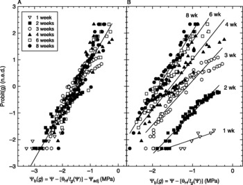
Probit regression analysis (Finney, Reference Finney1971) was performed on germination time course data (for 1% ≤ g ≤ 99%). As t g is the earliest time a specific germination percentage is observed, subsequent observation times, when no additional seeds germinated, were not included in the regression analyses. However, points for those observations are illustrated in Fig. 7. In the experiment with different afterripening times (see Fig. 4), this analysis was executed by either: (1) pooling data from subsequent afterripening times (Christensen et al., Reference Christensen, Meyer and Allen1996; see Fig. 4A), by regressing probit(g) on Ψb(g) calculated as [Ψ − θH/t g(Ψ)] − Ψadj, where Ψadj is the adjustment term, changing with afterripening time (it is the difference between the averaged value of Ψb and the actual Ψb value for each afterripening time); or (2) analysing datasets for each afterripening time separately (see Fig. 4B) and regressing probit(g) against Ψb(g) = Ψ − [θH/t g(Ψ)] (Bradford, Reference Bradford1990). Consequently, in the first case only, Ψb was allowed to vary with afterripening, while with the second approach, all the three parameters (Ψb, θH and σΨb) were permitted to change. Parameter optimization was conducted with the Curve Fitting routine of the SigmaPlot 2.0 software (Jandel Scientific, San Rafael, California, USA), which employed a least squares method.
Germination times at all incubation Ψs [t g(Ψ)] were normalized as germination times in water by multiplying by a correction factor (Bradford, Reference Bradford1990):

As the hydrotime model was applied to the viable seed fraction (Gummerson, Reference Gummerson1986), the graphics directly linked to it (see Figs 3, 4, 6, 7 and 11) report g, germination values corrected for viability; otherwise, the observed germination data are reported.
Germination index
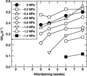
For SH96, time to 50% germination (t 50, median germination time) was graphically interpolated from Fig. 1 as the abscissa of the point at which each germination time course crosses that germination percentage. The rate to attain 50% germination (median germination rate) was determined as GR50 = 1/t 50 and is reported in Fig. 2 for treatments where 50% germination was achieved.
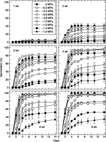
Germination time courses of red rice (SH96) incubated at different water potentials (0 to − 1.6 MPa) at 30°C in darkness, following 1, 2, 3, 4, 6 and 8 weeks of dry afterripening at 30°C.

Germination rates [GR50 = 1/t 50 = (Ψ − Ψb)/θH] for red rice (SH96) at different water potentials (0 to − 1.4 MPa) during incubation at 30°C, following dry-afterripening from 1 to 8 weeks. Symbols correspond to the water potential of the incubation medium (0 to − 1.4 MPa) during the first germination test at 30°C in darkness.

Results
The degree of afterripening determined the overall pattern of the germination time course; increasing time of afterripening produced higher final germination percentages (Fig. 1) and higher germination rates (Fig. 2) at each Ψ. Decreasing Ψ progressively reduced both final germination percentages (Fig. 1) and germination rates (Fig. 2) of red rice.
Hydrotime model
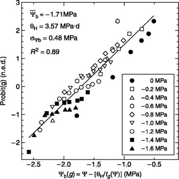
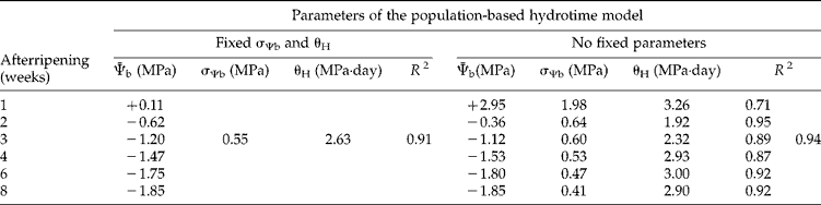
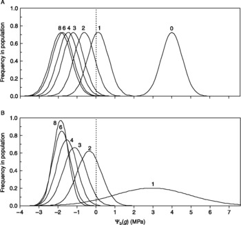
Probit regression analysis was performed on germination time course data for fully afterripened SH98 florets (Fig. 3) and for SH96 with different degrees of afterripening (Fig. 4). In the latter case, probit(g) was first regressed on [Ψ − θH/t g(Ψ)] − Ψadj (Christensen et al., Reference Christensen, Meyer and Allen1996), so that only Ψb was left to vary with afterripening. The probit regression line obtained in this way (Fig. 4A) showed a good fit, suggesting that the hydrotime model provided a satisfactory description of the data (R 2 = 0.91, Table 2), with Ψb accounting for differences among afterripened samples. To confirm this finding, the data from each afterripening time were also regressed separately, allowing all three parameters (Ψb, θH and σΨb) to vary among increasingly afterripened populations (Fig. 4B). Probit regression analysis of probit(g) versus Ψb(g) = Ψ − [θH/t g(Ψ)] reduced the data obtained at different Ψs to a linear, independent relationship for each afterripening time (Fig. 4B). In this case, changes in σΨb and θH, in addition to Ψb, were revealed during afterripening (Table 2; different slopes in Fig. 4B), which accounted for an increased ability of the model to describe the overall data variability, from 91 to 94% (see R 2 values in Table 2). The most relevant variation in such parameters was the change of σΨb between 1 and 2 weeks of afterripening, which was associated with a large change in Ψb over the same period (Table 2). The sample at 1 week of afterripening had the highest standard error for Ψb (see inset in Fig. 5) and the worst fit (R 2 = 0.71), but this was expected, as we sought to infer the parameters of the whole Ψb distribution from just a few germination data. Ψb showed an exponential decrease to − 1.85 MPa at 8 weeks of afterripening (Table 2, inset in Fig. 5), a value quite similar to that found for the fully afterripened SH98 sample ( − 1.71 MPa; Fig. 3). At 8 weeks of afterripening, the SH96 population showed both a slightly lower variability (σΨb = 0.41 MPa; Table 2) and a lower hydrotime constant (θH = 2.90 MPa·day; Table 2) than the SH98 population (σΨb = 0.48 MPa, θH = 3.57 MPa·day; Fig. 3). Figure 6 illustrates the shifting of the Ψb distribution, which moves past the 0 MPa point as afterripening time increases, allowing seeds to germinate. The shifting is apparent whether only Ψb (Fig. 6A) or all the three parameters, Ψb, θH and σΨb (Fig. 6B), were allowed to vary with afterripening time. The Ψb distributions well to the negative side of 0 MPa (afterripened seed) were relatively similar in the two cases, whereas strong differences occurred for dormant and partially afterripened seeds. Thus, only data from Ψb distributions across 0 MPa, i.e. those for 1 and 2 weeks of afterripening, are really useful to compare the two models. Therefore, although the overall R 2 of the model with three fluctuating parameters is only modestly higher than that of the model with only Ψb varying (Table 2), comparison of the Ψb distributions for 1 and 2 weeks of afterripening (Fig. 6A, B) to the corresponding germination plots (Fig. 1) suggests that the former model has a quite better agreement with observed germinations than the latter.
Probit regression of cumulative germination versus base water potential [Ψb(g)] for fully afterripened red rice (SH98). The g percentages were converted to probit(g) values (expressed in normal equivalent deviates, n.e.d.; Finney, Reference Finney1971). Percentages of 0 and 100 were omitted, as they correspond to infinite values for a Gaussian distribution. Regression analysis was conducted according to Bradford (Reference Bradford1990). Optimized hydrotime parameters are reported (θH, Ψb and σΨb are the hydrotime constant, the mean and the standard deviation of the base water potential distribution, respectively). Symbols correspond to the water potential of the incubation medium (0 to − 1.6 MPa) during the first germination test at 30°C in darkness.

Probit regression of cumulative germination percentages versus base water potential for red rice (SH96) dry afterripened for 1, 2, 3, 4, 6 and 8 weeks at 30°C. The g percentages were converted to probit(g) values (expressed in normal equivalent deviates, n.e.d; Finney, Reference Finney1971). Percentages of 0 and 100 were omitted, as they correspond to infinite values for a Gaussian distribution. Regression analysis was conducted by two procedures: (A) pooling data from subsequent afterripening times by regressing probit(g) on Ψb(g) calculated as Ψ − [θH/t g(Ψ)] − Ψadj, where Ψadj is the adjustment term, changing with afterripening time (it is the difference between the averaged value of Ψb and the actual Ψb value for each afterripening time). Only Ψb was allowed to vary with afterripening (Christensen et al., Reference Christensen, Meyer and Allen1996). In (B) datasets for each afterripening time were analysed separately, regressing probit(g) against Ψb(g) = Ψ − [θH/t g(Ψ)]. All the three parameters (Ψb, θH and σΨb) were permitted to change (Bradford, Reference Bradford1990). Symbols correspond to the time of dry afterripening (1–8 weeks at 30°C).

Hydrotime parameter estimations as obtained by optimization with the probit regression analysis*. Fixed σΨb and θH: data from subsequent afterripening times have been pooled (Christensen et al., Reference Christensen, Meyer and Allen1996; Fig. 4A), calculating Ψb(g) as [Ψ−(θH/t g(Ψ)]−Ψadj. No fixed parameters: datasets for each afterripening time have been analysed separately (Fig. 4B), regressing probit(g) against Ψb(g)=Ψ−[θH/t g(Ψ)] (Bradford, Reference Bradford1990)
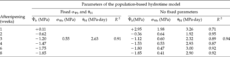
*The goodness of fit was evaluated by R 2 = 1 − (SSE/SST) for each linear regression, as well as for the overall fit of the probit regression model with ‘No fixed parameters’ to the actual data. SSE, error sum of squares; SST, total sum of squares.
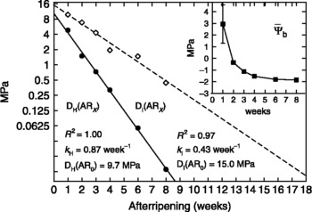
Values of DH(ARX), which represents a measure of dormancy of the seed population (in MPa) based on the hydrotime model [ = Ψb(ARX) − Ψb(ARN)], and DI(ARX), which represents an analogous measure of susceptibility to secondary dormancy induction [ = Ψind(ARX) − Ψind(ARN)], plotted on a natural logarithmic scale, versus time of afterripening. Lines are the linear regressions [for DH(ARX), weighted in proportion to the actual number of observations used to identify each point]. Inset: the decrease of Ψb during afterripening for red rice (SH96) (data reported in Table 2; error bars are shown when larger than the symbol and correspond to standard errors of the mean).

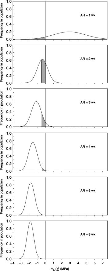
Theoretical distributions of base water potentials among red rice florets (SH96) after 0, 1, 2, 3, 4, 6 and 8 weeks of dry afterripening were predicted according to: (A) Christensen et al. (Reference Christensen, Meyer and Allen1996), with only Ψb varying with afterripening (probit regression as in Fig. 4A; parameters from Table 2); (B) Bradford (Reference Bradford1990), with all the three parameters (Ψb, θH and σΨb) changing for each afterripening time (probit regression as in Fig. 4B; parameters from Table 2). In (A), the value of Ψb for 0 weeks of afterripening was obtained by applying to the Ψb values calculated according to Christensen et al. (Reference Christensen, Meyer and Allen1996) the same kind of linear fitting used in Fig. 5 [ln DH(ARX) = ln DH(AR0) − k H·t AR]. Kinetic parameters were thus optimized also for this model [k H = 0.72 week− 1; Ψb(ARN) = − 1.858 MPa, R 2 = 0.98], and Ψb for 0 weeks of afterripening was derived from the extrapolation of DH(ARX) [DH(AR0) = 5.86 MPa]. In (B), the distribution for 0 weeks of afterripening was omitted as the value of σΨb is not known for afterripening times different from those measured. Each normalized Gaussian distribution has unitary area (equivalent to 100% germination), so that larger σΨbs imply lower frequencies around the mean.

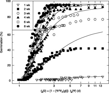
At each afterripening time, the germination time courses at different Ψs (Fig. 1) were normalized to match the corresponding time courses in water (Fig. 7) by multiplying the t g(Ψ) values by {1 − [Ψ/Ψb(g)]}, according to equation (equation (3)) (Bradford, Reference Bradford1990). Changes of θH, Ψb and σΨb, as a function of afterripening, resulted in corresponding differences in the normalized times to germination (Fig. 7; Dahal and Bradford, Reference Dahal and Bradford1990; Bradford, Reference Bradford, Kigel and Galili1995). This transformation also illustrates the discrepancies between the predicted (solid lines in Fig. 7) and the observed (symbols in Fig. 7) time courses at different times of afterripening. After an initial period of rapid germination, maximum germination plateaus (at < 90%) were reached for samples afterripened for 2 and 3 weeks (Fig. 7), essentially due to reduced germination from tests conducted in water.
Germination time courses of red rice (SH96) following different afterripening times (data from Fig. 1, corrected for viability) are plotted using a logarithmic scale for time, after normalization of t g(Ψ), the germination time at different water potentials, to t g(0), the time of germination in water [equation (3); Bradford, Reference Bradford1990]. This transformation illustrates the discrepancies between the predicted (solid lines) and the observed (symbols) germination time courses. Symbols correspond to time of dry-afterripening (1–8 weeks) at 30°C.

Application of other models
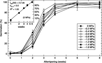
Data from germination tests in water were also analysed according to the model of Roberts (Reference Roberts1961a), describing a dormant seed population in terms of a normal distribution of dormancy periods [t AR(g), i.e. times of afterripening required by different fractions of the population to accomplish germination in a standard test]. The mean dormancy period [corresponding, for a fully dormant population, to t AR(50), the afterripening time to reach 50% germination], was then assumed as an index of dormancy (Roberts, Reference Roberts1961a). In red rice, the plot of total germination after 28 d of incubation in water at 30°C (14 d during the first treatment plus 14 d during the second one) versus afterripening is approximately sigmoidal (Fig. 8). However, it could be linearized only if probit germination was plotted against afterripening time on a natural logarithm scale (inset, Fig. 8), i.e. the cumulative t AR distribution (distribution of final germination percentages over different times of afterripening) was ln-normal rather than normal. For the same reason, the standard deviation of the distribution of mean dormancy periods, proposed to describe afterripening in barley (Favier and Woods, Reference Favier and Woods1993), could not be directly used to model red rice germination under these conditions.
Final germination percentages of red rice (SH96) after 2 weeks at different Ψs and 2 additional weeks in water at 30°C, following dry afterripening for 0, 1, 2, 3, 4, 6 and 8 weeks. Inset: data for incubation in water for 4 weeks (0 MPa) are plotted using a probability scale for germination percentages and a natural logarithmic scale for time of afterripening (weeks) (t AR); solid line is the linear regression.

A uniform dormancy index
The population-based hydrotime model can be used to describe the afterripening process through shifts in the Ψb distribution (Fig. 4B). In fact, the Ψb of non-dormant seeds represents the minimum Ψb for a given sample, and dormancy has been described as an increase over this basal value. However, such a basal value, by itself, is not related to dormancy, but rather to the intrinsic germinative vigour of the seed (Welbaum and Bradford, Reference Welbaum and Bradford1991; Bradford, Reference Bradford and Lang1996). Hence, from a theoretical point of view, the measure of dormancy on a Ψ scale, with 0 set to the water potential of pure water, does not represent the best way to deal with the concept of dormancy. To overcome these disadvantages, a uniform dormancy index can be obtained by subtracting the final value of Ψb (for the fully afterripened population) from the value of Ψb after each given afterripening period:

where DH(ARX) represents a measure of dormancy of the seed population (in MPa) based on the hydrotime model, Ψb(ARX) is the mean base water potential of the seed population at time X of afterripening, and Ψb(ARN) is the mean base water potential of the fully afterripened seed population, which is the lower limit of the exponentially decreasing curve shown in the inset in Fig. 5 [calculated to be − 1.854 MPa, i.e. the value that is optimized by iterative fitting in the linear regression of DH(ARX), Fig. 5]. In this way, the non-dormant population has a DH(ARX) = 0, and the relative dormancy status of the seed population is expressed by higher, always positive, values of this index on a Ψ scale.
Dry afterripening as an exponential decay
The shift of Ψb occurring during afterripening of red rice was not linear with respect to afterripening time, but it was higher initially and then decreased towards a limit that is observed for the fully afterripened seed population, seemingly following an exponential decline (Table 2; inset in Fig. 5). As the change in the dormancy status of the afterripening seed population is due to some unknown (bio)chemical change, it appears that whatever mechanism is involved, the unknown factors that prevent germination and cause dormancy would also show an exponential decay. If so, DH(ARX) represents a measure of the (bio)chemical change occurring during afterripening, and can be used to test the kinetics of the process (Atkins and Jones, Reference Atkins and Jones1997). When lnDH(ARX) is plotted against afterripening time, it fits first-order (or pseudo-first-order) reaction kinetics (solid line in Fig. 5), suggesting a decay process, described by [A]t = [A]0·e− kt or ln[A]t = ln[A]0 − kt (Atkins and Jones, Reference Atkins and Jones1997), where [A] is the concentration, in this case indirectly measured by DH(ARX), of the dormancy factor at times t and 0, and k is the kinetic rate constant. A kinetic rate constant (k H = 0.87 week− 1) and a half-life time (τH = 0.80 weeks) can then be calculated for the afterripening temperature employed in our experiment (30°C), as these values are, respectively, the slope of the straight line (with a change of sign) obtained by regressing lnDH(ARX) versus time (solid line in Fig. 5) and ln2/k H (Atkins and Jones, Reference Atkins and Jones1997). The rate of the afterripening process is v AR = k H·DH(ARX) (Atkins and Jones, Reference Atkins and Jones1997), i.e. the velocity of shift of the Ψb distribution during dry-afterripening (MPa week− 1) decreases as the process proceeds. At the same time, σΨb, the standard deviation of the Ψb distribution, also decreased (Table 2). A coherent explanation could be that an unidentified inhibitory factor (or factors) was present in dormant red rice in a quantity related to the depth of dormancy (measurable as changes in Ψb). While in non-dormant seeds its presence should be nil, this factor would increase with the depth of dormancy, and so should the value of its variance among seeds, becoming more and more a relevant contributor to the total population variance. Then, DH(ARX) and its inherent standard deviation,  , can be interpreted, respectively, as an indirect measure of the dormancy factor (whether it is an inhibitor, a metabolic modulator or a more complex process) and as a measure of variability in dormancy status among seeds.
Induction of secondary dormancy
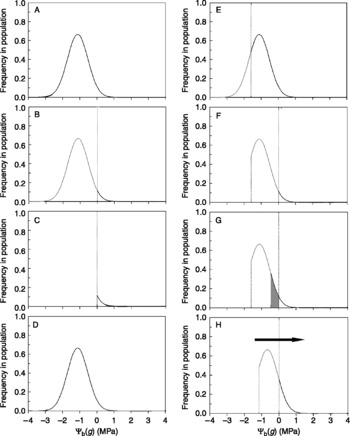
After incubation at different Ψs for 2 weeks (first treatment), all the ungerminated florets were transferred to standard germination plates with water (second treatment), and further incubated at 30°C for 2 weeks. Additional germination was achieved, depending upon the previous Ψ of incubation and time of afterripening (compare Figs 1 and 8), as the low Ψ had prevented the completion of germination during the first treatment. However, final cumulative germination percentages at the end of second incubation treatment, particularly following partial afterripening (2–4 weeks of afterripening), did not reach values that florets attained before incubation at low Ψs, and were reduced in proportion to the Ψ of medium during the first incubation (Fig. 8). As no differences in viability were found among treatments (data not shown), induction of secondary dormancy appeared to be responsible for this reduction. Figure 9 illustrates our interpretation of how incubation in low Ψ caused the ungerminated fraction of the seed population to backslide into dormancy again, i.e. secondary dormancy was induced.
The theoretical distribution of base water potentials after 3 weeks of dry afterripening (as from Fig. 6B) was used to illustrate the interpretation of the reduced germination observed after the second incubation (in water) as a consequence of low Ψ during the first incubation treatment. (A, B, C) incubation in water (Ψ = 0 MPa) during the first incubation treatment; (D–H) incubation at − 1.6 MPa (as an example Ψ) during the first incubation treatment. The solid line represents the portion of ungerminated seeds, and the dotted line represents the portion of seed that germinates, in the considered treatment. (A) The theoretical Ψb distribution before testing; (B) after the first incubation in water most seeds germinated; (C) the ungerminated seed fraction also remained ungerminated after the second incubation in water. (D) The same theoretical Ψb distribution before testing at lower Ψ; (E) reduced germination occurred after the first incubation at − 1.6 MPa; (F) the expected germination after the second incubation in water; (G) the observed germination after the second incubation in water, the grey area is the fraction of the seed population (as modelled in Fig. 11) that does not germinate when it was expected to; (H) this incongruence was interpreted as indicating that the Ψb distribution had shifted to higher water potentials during seed incubation at − 1.6 MPa.

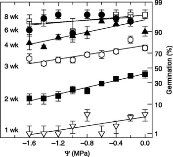
Final germination percentages could be linearized when plotted on a probability scale versus incubation Ψ (Fig. 10), revealing a normally distributed effect of water potential on induction of secondary dormancy. The inductive effect of Ψ was represented by the slope of the regression lines (Fig. 10), expressed as Δprobit(g)/ΔΨ [probit(g)/MPa]. As the slopes appeared approximately similar throughout the afterripening period, a given reduction in Ψ during the initial incubation resulted in a consistent fraction of seeds, in probit units, being induced into secondary dormancy. As a constant shift in terms of standard deviations represents different actual percentages of seeds affected at different places in the distribution, the linear relationship between probit germination and Ψ (Fig. 10) indicates that the actual change in germination percentage (maximal around 50% and minimal towards 0 and 100%) also depends upon germinative capacity of the sample; that is, the extent of afterripening. In other words, when the seed population gradually afterripens, the first and the last fractions of seeds that lose dormancy are, respectively, the ones at the more negative and less negative tails of the Ψb distribution, where re-induction of (secondary) dormancy would have a small relative effect on the observable germination. When Ψb approximates Ψ = 0 MPa and germinative capacity is around 50%, a similar change in the position of the whole distribution has a greater effect upon the observable germination (Finney, Reference Finney1971). This is also apparent as a greater spread among Ψ treatments at 2 and 3 weeks in Fig. 8.

The induction slopes (Fig. 10), analogous to the slopes in Fig. 4B, also represent a distribution of threshold water potentials. However, here the points refer to induction of secondary dormancy, and these are induction thresholds, Ψind(g). They constitute a distribution of minimum water potentials just permitting induction of secondary dormancy during the 2 weeks of incubation. The more horizontal the slope is, the smaller the effect of Ψ on induction of dormancy. The slopes of induction were less slanted (Fig. 10) than the slopes of the Ψb distribution (Fig. 4B), as only part of the fraction of seeds prevented from germinating was also induced into secondary dormancy over the first 14 d of incubation.
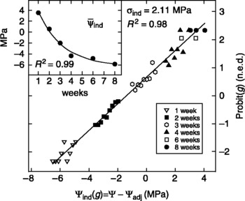
Assuming that negligible changes in the induction slopes occur during afterripening (Fig. 10), the decrease in inducibility should be entirely due to the upward shift of the induction line (towards higher germination percentages) with afterripening time. As this corresponds to a decrease of Ψind (the mean value of induction thresholds at each afterripening time, corresponding to the point on the Ψ axis where each induction slope crosses 50% germination), this parameter could be utilized as an indicator of secondary dormancy inducibility, similar to the use of Ψb for breaking of primary dormancy. Probit regression analysis, conducted analogously as in Fig. 4A to determine Ψb, was performed by pooling data across afterripening times (Fig. 11). It should be noted that the main differences between Fig. 4A and Fig. 11 are that, while the former considered germination time courses during the first test of germination at different Ψs (i.e. the ‘classical’ application of the hydrotime model), Fig. 11 used final germination data after the second test of germination in water. Hence, in Fig. 11 no differences in the final germination percentages within each afterripening period should have occurred among water potentials and no distribution of water potential thresholds should have been detected, were it not for the induction of dormancy during the first test. As a consequence, it should have not been possible to calculate means of the Ψind distribution (Ψind) (induction slopes in Fig. 10 could never be extrapolated to cross 50% germination if they were flat). The mean water potential thresholds that were nevertheless calculated have, then, a very different meaning with respect to the ‘classical’ hydrotime model; they describe a distribution of water potential thresholds for dormancy induction and are therefore mean induction thresholds (Ψind). The physiological meaning of these induction thresholds can be appreciated by considering that they provide a quantitative measure of the relationship between the Ψ at which the seed population was incubated during the first test and the intensity of induction into secondary dormancy, expressed in terms of probit(g) of the seed population. Although only induction thresholds for 2 and 3 weeks of afterripening were close to their extrapolated Ψind values, whereas the Ψind values extrapolated from the other induction thresholds were far from the actual water potentials used in the experiments, the elaboration in Fig. 11 shows how data from all the afterripening times can be combined to produce an approximate but sensible estimation of the general effect of incubation Ψ on the induction of secondary dormancy.
Probit regression of cumulative red rice germination at the end of two consecutive incubations (2 weeks at different Ψs, plus 2 weeks in water at 30°C) versus adjusted Ψind was conducted by pooling data from each afterripening time (analogous to Fig. 4A, Ψ of incubation during the first treatment was adjusted for Ψadj, i.e. the difference between the averaged value of Ψb and the actual Ψb value for each afterripening time). Inset: the calculated decrease of Ψind during afterripening; solid line is the exponential regression (y = 15.5 · e− 0.44·x − 6.29).

The calculated Ψind values indicated an exponential decrease (inset Fig. 11) of the susceptibility of the seed population to be induced into secondary dormancy (inducibility) as the population dry-afterripens. This fact can also be appreciated in relation to the ‘classical’ hydrotime Ψb distribution, as visualized in Fig. 12: the fraction of the seed population that is induced into secondary dormancy following incubation at − 1.6 MPa represents a progressively decreasing proportion of the whole seed population. An index, DI(ARX = Ψind(ARX) − Ψind(ARN), similar to DH(ARX), was then adopted as a measure of inducibility; so that a comparison with dormancy breaking became possible. The plot of DI(ARX) on a logarithmic scale showed that first-order kinetics apply to this property, as well (dashed line in Fig. 5). Ψind(ARN) was assumed to be − 6.29 MPa, the lower limit of the exponential regression (inset in Fig. 11), a value that predicts that a fully afterripened seed would not be readily susceptible to induction into secondary dormancy.
The theoretical distributions of base water potentials (as from Fig. 6B) were used to illustrate the effect of afterripening on the reduction of germination that occurred during the second incubation treatment because of prior incubation at − 1.6 MPa (as an illustrative Ψ). The grey areas represent the fractions of the seed populations (as modelled in Fig. 11) that do not germinate as they were expected to. This fraction is constant in probit terms across afterripening times (because Fig. 11 assumes the same slope, and then the same standard deviation of the Ψind distribution, for all the afterripening times). On the Ψ axis the width of the grey area decreases across afterripening times because the standard deviation of the Ψb distribution decreases during afterripening (Fig. 6B), so that each given seed fraction, in probit terms, corresponds to a smaller interval in Ψ terms.

The slope of the probit regression in Fig. 11 (i.e. 1/σind) indicates the effect of the Ψ value during incubation on the intensity of secondary dormancy induction (shift to higher Ψs, in n.e.d. units, of the Ψb distribution). Thus, it can be calculated that, in probit terms, the fraction of the distribution that backshifts past 0 MPa has a width of 0.47·Ψ (1 probit(g)/2.11 MPa), that is, it spans 0.76 n.e.d. units (standard deviations) from 0 to − 1.6 MPa. Because of the moving of the Ψb distribution during afterripening, this fraction appears to shift through the population, i.e. it will occur at different parts of the overall distribution as the Ψb(g) curve moves past 0 MPa. This is why points in Fig. 11 are grouped at each AR time. The moving of the Ψb distribution is shown in Fig. 12, where the grey area under the Gaussian distributions just to the left of 0 MPa represents the fraction of the distribution that backshifts past 0 MPa at each AR time (i.e. 0.76 ·σΨb; with different widths on the Ψ axis because σΨb varies during afterripening). Figure 12 also illustrates how, during afterripening, the fraction of seeds that germinates increases; the proportion of the seeds that should germinate, but do not germinate, decreases.
Discussion
Following afterripening, red rice expanded its germinative capacity in water and at lower water potentials (Fig. 1), simultaneously increasing the rate of germination (Fig. 2). Although rice was found to germinate only when soil had a water potential above − 0.8 MPa in the field (Hunter and Erickson, Reference Hunter and Erickson1952), under controlled conditions afterripened red rice can germinate c. 50% at water potentials of − 1.7 to − 1.8 MPa (Ψb in Fig. 3 and Table 2).
Increased germination rate has been observed as a component of dormancy breaking in grasses (Gordon, Reference Gordon and Heydecker1973). In Bromus tectorum seeds, even after full germination was achieved, mean germination time continued to decrease with afterripening, and longer storage was required to germinate uniformly than to germinate completely or quickly (Allen et al., Reference Allen, Meyer and Beckstead1995). In barley, the change in mean germination time on a logarithmic scale was normally distributed over the afterripening period, and could be modelled as a function of storage temperature and seed vigour (Favier, Reference Favier1995). Germination rate continued to increase after primary dormancy was lost, until it reached an upper limit determined by the intrinsic germinative vigour of the seed lot (Favier, Reference Favier1995). An afterripening period is also required to expand the temperature and water potential ranges allowing germination, and to achieve maximum germinability and vigour in muskmelon (Cucumis melo L.) (Welbaum and Bradford, Reference Welbaum and Bradford1991).
Population-based hydrotime model
Low Ψs influence germination rates and percentages by reducing seed water content and cell turgor (Welbaum et al., Reference Welbaum, Tissaoui and Bradford1990). Germination responses to reduced Ψ can be compared among different seed lots and treatments (Bradford, Reference Bradford1990; Dahal and Bradford, Reference Dahal and Bradford1990), according to the model first proposed by Gummerson (Reference Gummerson1986) and further extended by Bradford (Reference Bradford1990, Reference Bradford and Lang1996). The hydrotime model appeared to be a useful framework to describe red rice germination responses to reduced Ψ and to afterripening. Our results support the findings of Welbaum and Bradford (Reference Welbaum and Bradford1991), Christensen et al. (Reference Christensen, Meyer and Allen1996), Alvarado and Bradford (Reference Alvarado and Bradford2005) and Bair et al. (Reference Bair, Meyer and Allen2006): a change in Ψb of the dormant population can account for modifications in the germination time course as a consequence of afterripening. We also found that a generally increasing trend in θH values and a progressive reduction in the standard deviation of the Ψb distribution (σΨb) were associated with the afterripening process (Table 2). Although these changes in θH and σΨb improved the variation explained by the model by only 3%, we propose that the variation in σΨb is important, as its trend (a large initial decrement, followed by a smaller constant decline) paralleled that of Ψb (see above). Moreover, the model that assumes σΨb to be constant does not show a good fit to actual germination data of seeds that are partially afterripened; in fact, actual germination at 1–2 weeks of afterripening is less than this model would predict (compare Figs 1 and 6). In true potato seeds, a small change in σΨb, but a consistent increase in θH, was observed during afterripening (Alvarado and Bradford, Reference Alvarado and Bradford2005). However, we observed that the most significant reduction in σΨb occurred during the passage from almost no germination to approximately 50% germination in water (from 1 to 2 weeks of afterripening, Table 2), while in the experiment of Alvarado and Bradford (Reference Alvarado and Bradford2005), potato seeds were already germinating c. 50% before afterripening. On the other hand, while Alvarado and Bradford (Reference Alvarado and Bradford2005) observed a doubling of θH, red rice showed about a 50% increase of θH from 2 to 8 weeks of afterripening, possibly for the same reason suggested by these authors: a proportionally greater contribution of the time necessary for water uptake during imbibition (Phase 1), which is not directly linked to the dormancy status, but is observed when germination times approach their minimum.
Small reductions in germination percentages (Fig. 1) and rates (Fig. 2) were observed in pure water compared to a slightly lower Ψ (particularly − 0.2 MPa). This phenomenon was particularly evident in partially afterripened florets (Fig. 1, 3–4 weeks), for which further germination should be expected (solid lines in Fig. 7). Instead, germination reached a plateau after 3–4 d (symbols in Fig. 7; points on the plateau correspond to incubation in water). In muskmelon (Cucumis melo L.), a similar phenomenon, called high-Ψ-sensitivity, has been observed (Dunlap, Reference Dunlap1988; Welbaum et al., Reference Welbaum, Tissaoui and Bradford1990; Welbaum and Bradford, Reference Welbaum and Bradford1991), which was reversed by slight reductions in Ψ, increased O2 partial pressure and removal of covering structures (Dunlap, Reference Dunlap1988).
Interpretation of the afterripening process
Based upon the hydrotime analysis of red rice germination, the different stages of afterripening can be distinguished (Figs 4B and 6), and the relative dormancy level of a seed lot can be described in terms of its Ψb (Table 2; Christensen et al., Reference Christensen, Meyer and Allen1996; Alvarado and Bradford, Reference Alvarado and Bradford2005).
Although Ψb explains most of the effect of afterripening, so that it is valuable in ecological studies (Christensen et al., Reference Christensen, Meyer and Allen1996; Bauer et al., Reference Bauer, Meyer and Allen1998), the use of Ψb as a relative measure of dormancy has some drawbacks. For non-dormant seeds, Ψb assumes a negative value that depends upon the intrinsic germinative characteristics of the seed sample, such as sensitivity of germination to Ψ and vigour [equations (1b) and (3); Gummerson, Reference Gummerson1986; Welbaum and Bradford, Reference Welbaum and Bradford1991; Bradford, Reference Bradford and Lang1996], although it is assumed to be stable with respect to environmental effects (Allen and Meyer, Reference Allen and Meyer2002). As a consequence, two populations with the same Ψb could have a different degree of dormancy if they differ in their basal Ψb values. In addition, loss of primary dormancy and increase in germination rate have been found to be quantitatively linked (Favier, Reference Favier1995), and dormancy sensu stricto has been suggested to be part of a continuum in the acquisition of complete and rapid germination of the population (Gordon, Reference Gordon and Heydecker1973; Welbaum and Bradford, Reference Welbaum and Bradford1991; Bradford, Reference Bradford and Lang1996; Baskin and Baskin, Reference Baskin and Baskin1998; Alvarado and Bradford, Reference Alvarado and Bradford2005), but the use of Ψb does not represent the clearest quantification of this phenomenon. Instead, a dormancy index, DH(ARX), which shifts the Ψ-axis origin to the point of zero dormancy, provides a simple numerical expression of the continuum represented by the concurrence of changes in germinative capacity and germination rate as interpreted through the hydrotime model.
While an exponential decline similar to that observed for red rice (inset, Fig. 5) was observed for afterripening of Bromus and true potato seeds (Christensen et al., Reference Christensen, Meyer and Allen1996; Alvarado and Bradford, Reference Alvarado and Bradford2005), the introduction of the dormancy index, DH(ARX), has allowed a description of dry afterripening in terms of decay kinetics. As it is focused upon the dormancy continuum, DH(ARX = Ψb(ARX) − Ψb(ARN), is an absolute measure of dormancy and can then be used to compare the dormancy status among times, treatments and seed populations. As a consequence of interpreting afterripening in terms of reaction kinetics, the values of Ψb higher than 0 MPa (when the population is fully dormant) can be inferred by extrapolating the kinetic equation beyond this boundary of non-measurability (where germination does not occur at all and shifts of the population can not be detected). In this way the level of dormancy of the fully dormant population, DH(AR0), can be calculated from the intercept of regression at time zero (Fig. 5). Under constant temperature conditions for afterripening, a deeply dormant population can be afterripened until it becomes partially dormant and subjected to hydrotime analysis. The kinetic equation can then be used to infer Ψb at every point, including the initial value at the start of afterripening, Ψb(AR0).
Although the (pseudo) first-order kinetics can describe afterripening of red rice, they probably reveal only a synthesis of several component processes. Both the hull and the naked caryopsis have a role in rice dormancy (Roberts, Reference Roberts1961b; Cohn and Hughes, Reference Cohn and Hughes1981), and they need to be considered separately (Cohn and Hughes, Reference Cohn and Hughes1981). So, if the complete process is due to multiple components, with one being limiting, the kinetics observed in red rice might be due to the constraining step. The hull may operate as a physical barrier or by reducing oxygen availability to the seed (Roberts, Reference Roberts1961b, Reference Roberts1962), and the decay reaction could be a (non-enzymatic) oxidative process (Roberts, Reference Roberts1962; Leopold et al., Reference Leopold, Glenister and Cohn1988; Foley, Reference Foley1994) that, by reducing the oxygen availability to some metabolic oxidative reaction inside the seed, acts as a germination-inhibiting factor. Corbineau and Côme (Reference Corbineau, Côme, Kigel and Galili1995) reported that seed coats of many species are often responsible for limiting the rate of oxygen uptake, and proposed that polyphenols could be involved in the action of the external coverings. A similar conclusion was reached by Navasero et al. (Reference Navasero, Lyda and Juliano1975) for rice. Decay kinetics represents a general framework that could include any oxygen-mediated phenomenon wherein hulls could have some role.
Inferences from the hydrotime model
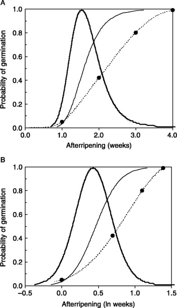
In the afterripening model developed for barley (Favier and Woods, Reference Favier and Woods1993), the rate of dormancy breaking in relation to dry-storage temperature has been described by the standard deviation of the germinability curve (σd), obtained by the probit transformation of germinability values plotted against afterripening time. The sigmoidal shape of dormancy loss curves and the inherent normal distribution of dormancy recovery periods among seeds were first appreciated in rice (Roberts, Reference Roberts1961a, Reference Robertsb, Reference Roberts1962). The probit transformation of those curves was performed, and the mean dormancy period [corresponding, for a normal distribution, to t AR(50), the median dormancy period, i.e. afterripening time to obtain 50% germination] was used to characterize seed afterripening (Roberts, Reference Roberts1961a, Reference Robertsb, Reference Roberts1962). According to the hydrotime model, this should correspond to the time for Ψb to become more negative than 0 MPa. Specifically, the afterripening time required for 50% of the seeds to become capable of germinating in water (i.e. the time for Ψb to shift to < 0 MPa on a Ψ axis), depends directly upon the value of Ψb itself and inversely upon the rate of afterripening, so that the median dormancy period is t AR(50) = Ψb/v AR. Analogously, Roberts (Reference Roberts1962) used the reciprocal of t AR(50) as a measure of the rate of loss of dormancy to study the kinetics of afterripening. More generally, the afterripening time required before a dormant fraction (g) can complete germination in water [t AR(g)] can be interpreted as the time needed for its water potential threshold [Ψb(g)] to shift below 0 MPa with a rate v AR (MPa week− 1). Therefore, the t AR distribution is perceived, from an intercept at 0 MPa on the Ψ-axis (test in water; dotted vertical line in Fig. 6), in relation to the speed at which Ψb(50) decreases: the higher is v AR, the more compressed the t AR distribution appears, and the smaller is its standard deviation (Favier and Woods, Reference Favier and Woods1993). In other words, if the Ψb distribution in Fig. 6A passes over the intercept at 0 MPa rapidly, this will require less time than if it passes slowly, producing, in the former case, a distribution of afterripening times that is consequently narrower than in the latter case.
In addition, if v AR is constant, the t AR distribution is normal (as it mirrors the Ψb distribution that is normal); however, in red rice afterripening, as the negative shift of the Ψb distribution slows according to first-order kinetics, the rate of increment in final germination percentage on a probit scale versus time of afterripening [Δprobit(g)/Δt AR] is gradually retarded (this can be visualized by the bunching up of the distributions on the left to 0 MPa in Fig. 6) and is ln-linear versus afterripening (reaction) time (inset, Fig. 8). In other words, when final germination is observed at a single water potential (classically Ψ = 0 MPa, i.e. germination tests in water), the first fractions accomplishing germination succeed faster than the ones that germinate after longer afterripening times, so that the normal Ψb distribution produces a skewed t AR distribution, which can be renormalized by adopting a ln scale on the time axis (inset, Fig. 8). This is illustrated in Fig. 13, where the t AR distribution was predicted from the Ψb distribution calculated according to Christensen et al. (Reference Christensen, Meyer and Allen1996). This trend should be true whenever the rate of the afterripening process rapidly decreases with decay kinetics. Consequently, while the median dormancy period [t AR(50)] can be used as a relative dormancy index (as it is linked to Ψb), σd loses precision when the t AR distribution is heavily skewed, and it should be substituted by a σln d value (standard deviation of the dormancy period distribution on a ln scale; inset, Fig. 8). Thus, two issues are demonstrated by Fig. 13: first, that skewness of the t AR distribution (and of the corresponding theoretical afterripening curve) is inherent to the decay kinetics of afterripening, and, second, that the hydrotime model as elaborated according to Christensen et al. (Reference Christensen, Meyer and Allen1996) does not match the actual afterripening curve, as this model underestimates the spread of afterripening times (σln d). Unfortunately, it was not possible to build up Fig. 13 with values from the analysis performed in Fig. 4B according to Bradford (Reference Bradford1990), because in such analysis σΨb is not fixed and it is not possible to model the changes of this parameter. However, as highlighted in Fig. 6, the greatest differences between the two models (Fig. 6A, B) are visible when the Ψb distribution passes across 0 MPa. Indeed, around this point, wider σΨb values (Table 2), and then a wider σln d, are predicted by the model of Bradford (Reference Bradford1990) with respect to that of Christensen et al. (Reference Christensen, Meyer and Allen1996).
(A) Theoretical t AR distribution (solid thick line) for germinative capability in water of unafterripened red rice seed (SH96), as predicted from the Ψb distribution (Fig. 6A) modelled according to the analysis of Christensen et al. (Reference Christensen, Meyer and Allen1996). The corresponding theoretical cumulative t AR distribution (solid thin line) and the observed cumulative g values (afterripening curve; dotted line) are also shown. To construct the t AR distribution, as v AR decreases exponentially with DH(ARX) during afterripening, the linearized regression of DH(ARX) was re-arranged as t AR = [ln DH(AR0) − ln DH(ARX)]/k H [parameters for the model of Christensen et al. (Reference Christensen, Meyer and Allen1996) as from the legend of Fig. 6] to obtain the predicted values of t AR from inputs in terms of Ψb(g). Then, the value of DH(ARX) at which Ψb(ARX) equals 0 MPa, that is − Ψb(ARN) [equation (4)], was obtained as described in the legend of Fig. 6A. In this way, the afterripening time that each g fraction requires to germinate in water [t AR(g)] was calculated from the value of DH(ARX) at which its Ψb(g) threshold passes 0 MPa, that is − probit(g)·σΨb − Ψb(ARN) {from equation (4) and equation (2) re-arranged as Ψb = Ψb(g) − [probit(g)·σΨb] with Ψb(g) set at 0 MPa}. (B) Time of afterripening was plotted on a logarithmic scale to re-normalize the t AR distribution.

This finding does not agree with the work of Roberts (Reference Roberts1961a), which showed a normal distribution of dormancy periods [t AR(g)s] for rice. In that case, v AR should be constant throughout afterripening; the afterripening process should then follow zero-order kinetics. A possible reason to explain this difference is that the t AR distribution is normal in indica varieties (Roberts, Reference Roberts1961a), while red rice is a weed with many characteristics of the cultivated japonica varieties, showing cross-pollination and phenotypic convergence with them (Hoagland and Paul, Reference Hoagland and Paul1978; Noldin et al., Reference Noldin, Chandler and McCauley1999). As differences in response to dehulling between the two subspecies have been described (Miyoshi and Sato, Reference Miyoshi and Sato1997), we can only speculate that the afterripening process also differs in some way between them.
Induction of secondary dormancy
Secondary dormancy can be induced by seed incubation at low Ψs (Khan and Karssen, Reference Khan and Karssen1980; Samimy and Khan, Reference Samimy and Khan1983; Kebreab and Murdoch, Reference Kebreab and Murdoch1999a). Many factors preventing seed germination are known to induce secondary dormancy (Baskin and Baskin, Reference Baskin and Baskin1998), and imposition of secondary dormancy has been proposed to affect the germination responses of some species and to occur simultaneously with the breaking of primary dormancy (Totterdell and Roberts, Reference Totterdell and Roberts1979; Cone and Spruit, Reference Cone and Spruit1983; Jones et al., Reference Jones, Ellis and Gosling1997; Kebreab and Murdoch, Reference Kebreab and Murdoch1999a). Since all of our experiments were performed in the dark to avoid light as a possible complicating and confounding factor for dormancy breaking (Roberts, Reference Roberts1962), the induction of secondary dormancy, which requires darkness (Totterdell and Roberts, Reference Totterdell and Roberts1979; Khan and Karssen, Reference Khan and Karssen1980), was made possible. Totterdell and Roberts (Reference Totterdell and Roberts1979) suggested that the loss of primary dormancy and the induction of secondary dormancy are independent processes that are normally distributed within the seed population, so that they can be represented by cumulative normal distributions. However, Samimy and Khan (Reference Samimy and Khan1983) also proposed that the differences between primary dormancy and secondary dormancy could be quantitative rather than qualitative. In this way, primary and secondary dormancy, due to the same or different mechanisms, should act in similar manners upon the seed population, as represented by the population-based hydrotime model.
In our experiments, secondary dormancy was induced in partially afterripened seeds during the 2 weeks of dark incubation at different Ψs, as revealed by the subsequent test in water (Figs 8, 10). The measurable effects of dormancy induction were differential germination with respect to 0 MPa (Figs 8, 12). Two main factors influenced this event: the time of afterripening and the value of incubation Ψ during the first treatment (the lower the water potential, the greater the induction; Figs 8, 10, 12). The relationships between final germination percentages and Ψ during the first incubation could be linearized by adopting a probability scale for germination (Fig. 10). This means that the extent of dormancy re-imposition that occurred during the first treatment (percentage of induction on a probability scale) was directly proportional to the fraction of the Ψb distribution that was prevented to germinate, at each incubation Ψ with respect to water (having Ψ < Ψb(g) < 0 MPa), and that a part of this fraction had its Ψb(g) increased >0 MPa (as it was no longer able to germinate in water). This suggests that induction of secondary dormancy acted as a backshift of the Ψb distribution (actually of the ungerminated fraction of the seed population) on the Ψ axis (Figs 9, 12).
In contrast to the increasingly angled slopes of the Ψb distribution (Fig. 4B; decreasing σΨb in Table 2), the regression slopes expressing induction of secondary dormancy (Fig. 10) showed no relevant change during afterripening. As in the hydrotime model, the slopes represent the distribution of Ψb thresholds in the seed population. It follows that while an increasing proportion of the seed population acquires germinative capability during afterripening, a constant portion, in probit terms, of the whole seed population is induced into secondary dormancy at each given incubation Ψ (Fig. 12). Hence, during afterripening the proportion of seeds that becomes secondarily dormant because of incubation at low Ψ (grey area in Fig. 12) decreases with respect both to the whole seed population (the whole area of the Ψb distribution), and to the fraction of seeds that had acquired the ability to germinate (the area of the Ψb distribution that is to the left of 0 MPa). Analogously, the proportion of seeds induced into secondary dormancy (grey area in Fig. 12) decreases with respect to the fraction of seeds that had been prevented from germinating during the first test by the low incubation Ψ (i.e. − 1.6 MPa in Fig. 12). Thus, inducibility (i.e. susceptibility to be induced into secondary dormancy) should just be proportionally higher for higher levels of primary dormancy (i.e. shorter afterripening times in Fig. 10). In fact, Ψind decreased exponentially during afterripening (Fig. 11). Accordingly, the inducibility index DI(ARX) [which, analogous to DH(ARX), is an actual measure of inducibility] revealed that inducibility into secondary dormancy follows an exponential decay, analogous to what was observed by using DH(ARX). The lower kinetic constant for the loss of inducibility, with respect to primary dormancy breaking (k I < k H, Fig. 5), indicated a slower decrease of secondary dormancy inducibility during afterripening (less angled regression slope, dashed line in Fig. 5). Moreover, while Ψb is defined independently from test duration, Ψind, as established here, reflects inducibility of dormancy specifically over a 14-d incubation. If, as probable, more secondary dormancy should be induced with longer incubations, the induction slopes would become more slanted, and the two straight lines in Fig. 5 would diverge further. Indeed, with afterripening, DI(ARX) reveals that the seed loses exponentially the capacity to undergo secondary dormancy. However, DI(ARX) indicates that such ability is lost more slowly than primary dormancy, suggesting that loss of primary dormancy and the loss of secondary dormancy induction are different aspects of the same decay process or they correspond to similar but distinct processes.
In summary, the present experiments describe the loss of dormancy in red rice via afterripening according to a population-based hydrotime model, confirming that increasing germinative capacity and germination rate are concomitant effects. An index, DH(ARX), derived from hydrotime analysis, has been introduced and suggested to represent an absolute measure of dormancy. Induction of secondary dormancy in red rice during dark incubation has been shown to be proportional to the water potential of the initial incubation medium. The inducibility of secondary dormancy has been expressed as an index, DI(ARX). Finally, in red rice, both primary dormancy breaking and secondary dormancy inducibility follow decay kinetics during afterripening. The decay curve and the index DH(ARX) could be tested in other species; the induction of secondary dormancy should be tested in relation to the time of incubation at low water potential(s); and the induction of dormancy in rice could be studied in the presence of abscisic acid, or at non-permissive sub-optimal temperatures for germination that are above the temperatures that induce dormancy-breaking by stratification.
Acknowledgements
This research was supported in part by Regional Research Project W-168. A.G. was supported by a fellowship from the National Research Council of Italy. F. David Gatz provided able assistance in the laboratory. We appreciate the critical evaluation of the manuscript by Dr Phil Allen, Brigham Young University, prior to its submission, and the detailed comments and patience of Dr Kent Bradford (monitoring editor) and the peer reviewers after submission of the paper. Approved for publication by the Director of the Louisiana Agricultural Experiment Station as paper 05-38-0446.