1. Introduction
Tactile sensors serve a crucial role for humans and robotics alike, acting as receptors that perceive external stimuli for decision-making and control signals [Reference Wang, Hu, Zhu, Huang, Wang, Li, Yang, Yu and Deng1, Reference Wang, Liu, Shang, Niu, Ke, Zhang, Ma, Li, Sun and Zhang2]. Soft tactile sensors, in particular, are gaining prominence due to the evolution of soft robotics, having promising potential in various applications [Reference Qu, Mao, Li, Xu, Zhou, Cao, Fan, Xu, Liang, Liu, Wang and Wang3, Reference Lin, Wang, Zhao, Xu, Wang, Zhang, Sun, Lin and Peng4]. Normally, these sensors leverage the flexibility of soft materials to detect external stimuli by measuring physical changes resulting from the material’s deformation through embedded sensing components within the soft body. This soft tactile sensor configuration can encompass a variety of sensing elements, including capacitive sensors [Reference Sarwar, Ishizaki, Morton, Preston, Nguyen, Fan, Dupont, Hogarth, Yoshiike, Qiu, Wu, Mirabbasi and Madden5], strain gauges [Reference Trinh, Ho and Shibuya6], piezo-resistive elements [Reference Gariya, Kumar and Prasad7], pressure sensors [Reference Lv, Tian, Jiang, Dang, Liu, Duan, Li, Chen and Xie8], fiber optic sensors [Reference Sepehri, Helisaz and Chiao9], magnetic sensors [Reference Dai, Zhang, Pan, Hu, Ji, Sun, Lyu, Tang, Li, Fu and Zhao10], or based on integration of vision and tactile sensing [Reference Xiong, Huang, Yin, Zhang and Song11]. These elements are strategically positioned within soft bodies based on specific sensing tasks, leading to the creation of soft bodies with diverse shapes like circular, flat, or dome structures. In which, dome tactile sensors or soft probes are the most common form, designed to effectively detect and measure contact forces, surface textures, and material properties. Their key advantages include adaptability to complex surfaces, high sensitivity to small force variations, and versatility in applications like robotic manipulation and medical diagnostics [Reference Zhao, Nguyen, Hoang, Do and Phan12–Reference Gomes, Lin and Luo15].
However, tactile sensors face significant drawbacks and challenges. Primarily, the main challenge in computing sensor output arises from two factors: The intrinsic physical nonlinearity of soft materials and the geometric nonlinearity caused by the large deformations of the soft body. Second, the low elastic modulus characteristic of soft materials restricts soft tactile sensors to a specific range of applied force. Beyond this range, excessive deformations occur, leading to issues such as hysteresis and nonlinearity, which affect the sensor accuracy. In addition, to detect various sensing tasks, multiple distinct sensing elements need to be deployed, leading to complexities in design, manufacturing, and signal processing to interpret the signals from these sensors [Reference Zhong, Zhao, Liu, Li, Kan and Feng16, Reference Kim, Lee, Hong, Shin, Kim and Park17]. Recently, leveraging morphological computation, which exploits the capability to modify attributes like shape, hardness, and softness, presents notable advantages in the realm of soft robotics, ranging from manipulations to soft sensors [Reference Stroppa, Majeed, Batiya, Baran and Sarac18, Reference Shan, Xu and Li19]. In this approach, soft tactile sensors can alter their morphology, enabling flexible adaptation to various interacting objects without the need for multiple sensor components [Reference Hughes, Scimeca, Maiolino and Iida20, Reference Trinh and Xuan21]. This advancement is particularly significant for applications involving soft materials, where precise interaction is often critical. Soft materials, especially those used in biomedical contexts, often have low elastic modulus values that are difficult to measure accurately. In such cases, soft tactile sensors must ensure an appropriate contact force to avoid damage or excessive deformation during interaction. Moreover, when tasked with detecting abnormally hard regions beneath layers of biomedical material—such as identifying tumors or defects—the sensor needs to maintain sufficient stiffness to penetrate soft material layers and make contact with the target regions. Morphological computation, with its ability to dynamically adjust stiffness, offers a versatile solution for addressing these diverse tasks. As a result, soft tactile sensors can efficiently determine the mechanical properties of soft materials, including elastic modulus and localized hardness variations.
From above issues, this study introduces a dome-probe-type soft tactile sensor capable of autonomously adapting its stiffness to evaluate the properties of contact objects. The probe features a hollow chamber with an appropriate wall thickness, allowing compressed air injection to induce initial pre-stress in the soft membrane, stretching it without significantly altering its geometry. This controlled adjustment primarily facilitates morphological adaptation through stiffness modulation, enabling the probe to perform diverse sensing tasks effectively. Using a single strain sensor element positioned at the probe’s tip, the proposed sensor can estimate parameters, including the elastic modulus, the depth of abnormally hard defect within soft material layers and the contact force. This eliminates the need for multiple sensor elements and reduces system complexity. To enhance the accuracy of predicting sensor outputs, the proposed system employs a hybrid approach combining numerical simulation and machine learning. Contact models are first solved using a simulation framework, where parameters are adjusted to match experimental conditions. The resulting strain data at the probe’s tip are calibrated with experimental data, then used to generate a dataset for training machine learning algorithms.
To estimate object properties such as shape, texture, and hardness, various soft tactile sensors have been developed. Among them, vision-based tactile sensors like GelSight have demonstrated remarkable performance in capturing high-resolution surface details and estimating object hardness [Reference Yuan, Srinivasan and Adelson22]. However, these approaches rely on optical feedback, which may limit their effectiveness when assessing subsurface material properties in non-transparent media. In addition, this soft tactile sensor operates with fixed stiffness properties, limiting its ability to adjust to different sensing tasks.
Several recent works have explored adaptable morphology and tunable stiffness in tactile sensors, but our approach differs in key aspects. For instance, Qi et al. [Reference Qi, Hirai and Ho23, Reference Qi and Ho24] introduced a wrinkled soft sensor inspired by water-induced wrinkles in human skin, which adapts its morphology through passive mechanical deformation (i.e., wrinkling) during stretching or bending. Their system enhances sensitivity to surface-level stimuli, especially in detecting tangential sliding or normal indentations. Two actuation strategies were demonstrated stretching and bending to allow passive morphological adaptation. In contrast, our sensor employs active stiffness modulation via pneumatic actuation, which makes it possible to flexibly adjust the sensor’s softness or stiffness, depending on the material being tested. This distinction is critical: passive wrinkling provides no control over indentation depth or how contact force is distributed across varying material properties. In our design, stiffness can be actively tuned to probe materials with different resistance levels, which directly affects the sensor’s ability to access and quantify subsurface information. More importantly, while Qi et al. primarily focused on improving contact sensitivity, our work is aimed at quantitative mechanical characterization, specifically estimating the elastic modulus and detecting subsurface anomalies. These objectives require fundamentally different sensing strategies. Our approach combines pneumatic stiffness control with strain-gauge sensing to directly capture deformation mechanics under different loading conditions, enabling the evaluation of material properties. This capability is crucial in applications like soft tissue diagnostics or material testing, where sensitivity alone is insufficient. Similarly, He et al. [Reference He, Herzig, Nanayakkara and Maiolino25] developed a tunable-stiffness sensor for surface texture detection, while our design integrates a soft membrane with strain-gauge sensing for subsurface stiffness analysis.
Bewley et al. [Reference Bewley, Jenkinson and Tzemanaki26] developed an optical-tactile sensor using pneumatic control to detect lumps in soft materials, particularly for medical applications like tumor detection. While their optical-tactile sensor also uses pneumatic control for stiffness modulation, their sensing mechanism heavily relies on camera-based optical feedback. This introduces several inherent limitations, such as sensitivity to ambient lighting, the need for careful calibration, and reduced performance in non-transparent or light-scattering materials. In addition, optical systems often demand substantial computing power to process images, which can slow down performance, especially in applications that require real-time responses. Using a camera also adds complexity to the system, making it larger, heavier, and harder to fit into compact or wearable robots. This makes such systems less suitable for settings where space and energy are limited. In contrast, our sensor utilizes strain-gauge-based sensing, which directly measures mechanical deformations and allows for direct acquisition of tactile data. This design eliminates the need for optical tracking, making our system more suitable for subsurface stiffness estimation, especially in soft and non-transparent materials. By focusing on direct mechanical signal acquisition, our sensor is compact, lightweight, and more easily integrated into soft robotic systems or medical devices. Moreover, the use of strain gauges reduces the computational complexity compared to camera-based systems, enabling faster and more reliable real-time performance. Overall, our design offers a more straightforward, and adaptable approach to subsurface stiffness measurement and elastic modulus estimation, distinguishing it from existing systems based on optical feedback.
In summary, while prior studies have explored stiffness-tunable and morphology-adaptive sensors, our work stands out by integrating active stiffness control with direct mechanical sensing for quantitative elastic modulus estimation and subsurface defect depth detection. These features make our design highly suitable for applications requiring accurate mechanical property evaluation, such as biomedical diagnosis and soft material inspection. Additionally, our approach combines theoretical modeling, numerical simulation, and experimental analysis to create a large training dataset. This hybrid methodology allows for efficient sensor training while minimizing the time and cost associated with prototype fabrication and experimental procedures.
2. Idea, design, and fabrication of a soft tactile sensor system
2.1. Idea
Inspired by the structure of human skin and fingers, where sensory organs beneath the skin and epidermis detect contact characteristics through pressing and sliding, humans can perceive the hardness and properties of objects. Depending on the contact object’s characteristics, the hand adjusts pressing force, depth, and deformation by changing the stiffness of its skeletal structure [Reference Jenkins and Lumpkin27–Reference Pleger and Villringer29]. Based on this concept, the soft tactile sensor system developed in this study is designed to mimic this adaptive capability by adjusting its stiffness using pneumatic pressure. This tunable stiffness mechanism enables the sensor to interact effectively with a wide range of materials, improving its ability to measure mechanical properties across different contact scenarios. A strain gauge-sensing element, embedded deep within the soft material layer, acts as the primary sensing unit to detect surface characteristics based on strain measurements.
2.2. Design
The soft probe-tactile sensor design consists of three main components: a rigid frame, a soft probe, and a sensing element, as shown in Figure 1.
Design of soft tactile sensor.

The structure of rigid frame and its dimensions depicted in Figure 2, in which its lower part is designed to house and secure the soft probe, while the upper part facilitates the connection of pneumatic pipes and sensor signal wires, and ensures convenient handling of the entire sensor system.
The soft probe is placed in the lower compartment of the rigid frame and consists of two parts. The main part, forming the lower body, is a hemisphere made of a soft material with a low elastic modulus, allowing it to deform easily under contact force. Furthermore, the hemisphere is hollow, allowing compressed air to be pumped in, inducing initial pre-stress, thereby adjusting the hardness of the soft probe. The connecting part, located between the lower body and the rigid frame, forms the upper body of the probe and is made of a soft material with greater hardness. This ensures rigidity, allowing only the hemisphere to deform under contact forces. A highly sensitive bridge-type strain gauge sensor, BX 120-3AA,Footnote 1 is centrally positioned 1 mm below the hemisphere’s top to measure the probe’s strain during contact.
Design of rigid frame.

2.3. Fabrication
The hard frame of the sensor is fabricated using a 3D printing method, while the lower body of soft probe is made from Ecoflex 20 silicone material, using a molding method. The mold for fabricating the soft probe consists of three main components: the base, the body, and the core. The base serves to securely position the mold body and core on a flat surface during the pouring process of the soft material. The mold body is made of two identical halves, featuring a hemispherical shape at the bottom and a square base at the top. The top square base has grooves for connecting to the core and threaded holes on its “ears” to join two halves via screws. This design ensures a tight seal when the body is placed into the hole on the base, preventing leaks during material pouring. The core, placed inside the mold body, creates a uniform gap of 2 mm between itself and the body. This gap is where the soft material is poured to form a thin-walled soft probe. The core’s top includes a square pillar
 $(5 \times 5 \times 1$
mm) to create a corresponding hole in the soft probe. This hole is used to mount the strain gauge sensor. After assembly, the base, body, and core structure are shown in Figure 3. The specific manufacturing process of the sensor system can be summarized as follows:
Step 1: The rigid frame and molds for pouring the soft material are produced using a 3D printing method.
Step 2: Attach the body and core to the base to form the bonding mold, as shown in Figure 3. Next, mix the Ecoflex 20 silicone (Parts A and B) in a 1:1 mass ratio. After mixing, degas the mixture, pour it into the gap in the bonding mold, and cure it in a heat chamber at
 $60^{\circ}$
C for 50 minutes. Once the material is solidified, remove the mold to get the soft probe body. Note that, after finishing this step, the probe body has a 1 mm deep hole on its inner wall. This hole is where the strain gauge sensor will be placed and fixed. The soft body with the strain gauge sensor positioned in the 1 mm hole is then placed onto a fixed base. The Ecoflex 20 liquid silicone mixture is poured into the hole to secure the strain gauge in the center of the soft body. After the liquid silicone dries, the complete soft body is formed, with the strain sensor positioned approximately 1 mm from the outer surface. Next, place the fully formed soft body into the groove in the middle of the lower compartment of the rigid frame. Then, pouring Dragon Skin 30, a harder silicone mixture, into the gap between the soft body and the rigid frame. Once this mixture has cured, the soft body is securely held in place on the rigid frame, with the upper body encased in the harder material. This ensures that only the lower hemisphere of the soft body deforms under contact pressure.
Step 3: The final assembled sensor system.
Assembly mold for fabricating soft proble.

3. Contact model of soft probe
To clarify the working principle of the sensor system, in the next section, we present a contact model of the soft sensor.
According to the Hertz contact model [Reference Dintwa, Tijskens and Ramon30, Reference Wu, Lin and Juang31] , when a soft probe makes contact with a soft flat plate under the press of a normal force
 $F$
, both the probe and the soft plate will undergo deformation in the normal direction by contact depths of
 $\delta _1$
and
 $\delta _2$
, respectively, as illustrated in Figure 4. The pressure distribution in the contact area is determined by the formula:
 \begin{equation} p = {p_0}{\left \{ {1 - \left ( {\frac {{{r^2}}}{{{a^2}}}} \right )} \right \}^{{\raise 0.7ex\hbox{$1$} \!\mathord {\left / {\vphantom {1 2}}\right .} \!\lower 0.7ex\hbox{$2$}}}} \end{equation}
A schematic contact model of soft probe and stress distribution.

where
 $r$
represents the distance from the center of the contact surface to the calculated stress point, and
 $a$
is the radius of the contact surface (assuming the contact area is circular and symmetrical). The maximum contact pressure occurs at the center of the contact area (
 $r = 0$
). The maximum contact pressure
 $p_0$
and the radius of the contact surface
 $a$
are determined using the following formulas:
 \begin{equation} {p_0} = \frac {{3F}}{{2\pi {a^2}}} \end{equation}
 \begin{equation} a = {\left ( {\frac {{3FR}}{{4{E^*}}}} \right )^{\frac {1}{3}}} \end{equation}
where
 $E^*$
is the effectiveness Young modulus, which depends on the mechanical properties of two contacting objects, determined as follows:
 \begin{equation} \frac {1}{{{E^*}}} = \frac {{1 - \upsilon _1^2}}{{{E_1}}} + \frac {{1 - \upsilon _2^2}}{{{E_2}}} \end{equation}
where
 ${E_1},{E_2}$
,
 $\upsilon _1$
, and
 $\upsilon _2$
are the Young modulus and Poison ratio of the soft probe material and soft plate material, respectively. And the equivalent radius of curvature
 $R$
is calculated as
 \begin{equation} \frac {1}{R} = \frac {1}{{{R_1}}} + \frac {1}{{{R_2}}} \end{equation}
where
 ${R_1},{R_2}$
curvature radius of soft probe, and soft plate, respectively. In a case of the flat soft plate,
 ${R_2} = \infty$
, thus:
 $R = {R_1}$
. The total normal deformation is determined as follows:
 \begin{equation} \delta = {\delta _1} + {\delta _2} = {\left ( {\frac {{9{F^2}}}{{16R{{\left ( {{E^*}} \right )}^2}}}} \right )^{\frac {1}{3}}} \end{equation}
The normal contact depths
 $\delta _1$
and
 $\delta _2$
can be estimated as
 \begin{equation} \delta _1 = \displaystyle\frac {\displaystyle\frac {1-\nu _1^2}{E_1}}{\displaystyle\frac {1-\nu _1^2}{E_1} + \displaystyle\frac {1-\nu _2^2}{E_2}} \cdot \delta \end{equation}
 \begin{equation} \delta _2 = \displaystyle\frac {\displaystyle\frac {1-\nu _2^2}{E_2}}{\displaystyle\frac {1-\nu _1^2}{E_1} + \displaystyle\frac {1-\nu _2^2}{E_2}} \cdot \delta \end{equation}
Equations (7) and (8) show that:
If
 $E_1 \lt E_2$
(the soft probe is softer than soft plate), most of the deformation will occur in soft probe, and
 $\delta _1 \gt \delta _2$
.
If
 $E_2 \lt E_1$
(the soft plate is softer than the soft probe), most of the deformation will occur in soft plate, and
 $\delta _2 \gt \delta _1$
.
From the above formulas, it is clear that the stress distribution depends on the elastic modulus of both the soft probe and the contact object. Therefore, the elastic modulus of the contact object can be determined based on evaluating the contact stress distribution or the deformation of the soft probe. Additionally, the maximum stress value
 $p_0$
and the total deformation of both the probe and the contact object not only depends on the contact force
 $F$
but also on the equivalent elastic
 $E^*$
. By adjusting the equivalent elastic modulus
 $E^*$
, it is possible to modify the stress
 $p_0$
and the contact depth
 $\delta$
. This suggests that to detect defects located deep beneath the surface of the contact object, the soft probe must have a high equivalent stiffness (
 $E_2 \lt E_1$
) so that the contact depth
 $\delta _2$
is sufficient for the probe tip to reach the defect location. This will cause a sudden change in the contact stress distribution when the probe passes over the defect, allowing the defect’s position can be identified. Whereas, when the elastic modulus of the contact surfaces needs to be determined, the probe should maintain a low elastic modulus or stiffness, to maximize the deformation (
 $\delta _1$
) and stress of soft probe during the contact process, thereby increasing the probe’s sensitivity. Based on this analysis, the proposed soft probe sensor is designed to adjust its equivalent stiffness to serve multiple purposes, including estimating the elastic modulus of soft contact objects and determining the depth of defects within soft materials. In the proposed design, the stiffness of the soft probe is actively modulated by controlling the level of pneumatic pressure injected into its hollow chamber Figure 1(a). As the internal air pressure increases, the silicone membrane undergoes pre-stress, altering its stiffness to enable precise defect depth estimation.
Based on the equation (6), the effectiveness modulus is calculated as follows:
 \begin{equation} {E^*} = \sqrt {\frac {{9{F^2}}}{{16R\delta }}} \end{equation}
Then from the equation (4), the Young modulus of the soft probe material can be estimated as
 \begin{equation} {E_1} = \displaystyle\frac {{1 - \upsilon _1^2}}{{\displaystyle\frac {1}{{{E^*}}} - \displaystyle\frac {{1 - \upsilon _2^2}}{{{E_2}}}}} \end{equation}
The equations (9) and (10) will be used to evaluated the equivalent stiffness of the soft probe under different pressure values in the section 4.4.1.
4. Analysis of sensor capability
The proposed sensor is designed to detect the elastic modulus of soft plates and the depth of abnormal hardness within soft material layers. This is achieved by assessing the stress at the contact point of the soft dome, measured through the strain of a strain gauge, which outputs a voltage signal. However, modeling the deformation of the strain gauge in response to varying contact characteristics and forces presents a significant challenge. To address this, we employed a machine learning approach; however, acquiring a large and diverse dataset to cover various contact scenarios is resource-intensive, requiring significant experimental costs and time for sample fabrication and testing. To overcome these challenges, we propose a hybrid approach that combines experimental and simulation data. In this method, simulation parameters are automatically adjusted to reduce execution time, and the resulting simulation data are aligned with the corresponding experimental data, using machine learning techniques. This integration creates a synchronized dataset that is large enough and comprehensive to effectively train the sensor system. Essentially, simulations serve as virtual experiments that significantly expand the dataset while reducing data collection time. The detailed methodology and implementation process are described in the following sections.
4.1. Experiment
To gather data for sensor training and synchronizing with simulation data, experiments were first conducted with the soft sensor system and various contact objects. These experiments were performed on the Universal Micro Material Tester (UMT) system.Footnote 2
In the experimental setup, the soft probe sensor was mounted on a vertical sliding table, serving as the upper sample (Figure 5). The lower samples consisted of soft plates made from various materials, and hard circular objects embedded beneath the soft layers to simulate different defects. The soft plate is rectangular, measuring
 $90 \times 70 \times 30$
mm in length, width, and height. These plates are fabricated from various types of soft silicone materials, including Dragon Skin 30, Dragon Skin 20, Dragon Skin 10, Ecoflex 30, Ecoflex 20, and Ecoflex 10. The molding process used to fabricate these plates is identical to the method employed for manufacturing the sensor system. On the soft plate’s surface, circular holes with diameters of
 $1, 2, 3, 4, 5, 6$
, and 7 mm are created. Then, hard spheres of corresponding sizes are placed into these holes to simulate subsurface defects.
Experimental setup.

To vary the depth of the defects, thin plates, each 1 mm thick and made from the same material as the soft plate, are glued to its surface. By stacking different numbers of these thin plates, the defect depth is adjusted from 1 mm to 7 mm. Once the thin plates are affixed, the soft plate contains embedded defects. These plates with defects serve as lower samples in the experiments. They are mounted onto the lower sliding table using a bracket manufactured via 3D printing.
The soft plates used in this study were fabricated from Dragon Skin and Ecoflex silicone materials, which exhibit mechanical properties similar to those of soft biological tissues. This allows us to assess the potential applicability of the proposed sensor in biomedical research, particularly in diagnostic and tissue characterization applications.
The experimental procedure is summarized as follows: The soft sensor, which is mounted on a load cell, is controlled by the UMT system software to regulate its sliding velocity and the contact force with the lower plate. Pneumatic pressure is adjusted using a solenoid valve system and a pressure regulator. Data from the strain gauge sensor are obtained via the LMS multi-channel signal system, which can simultaneously collect signals from 16 channels at high frequency.Footnote 3 The obtained data are stored as an excel file. Specific experimental parameters are as follows:
To determine the elastic modulus of the lower plate: Contact forces: 1 N, 1.5 N, 2 N, and 2.5 N. Sliding velocity: 10 mm/s. Movement time: 5 s. Total number of experimental cases: 30.
To identify abnormal hard positions: Contact forces: Same as above. Sliding velocity: 3.5 mm/s. Sliding time: 20 s. Sample depths for abnormal hard positions: Ranging from 1 mm to 7 mm. Total number of experimental cases: 48.
Pneumatic pressure levels: For the elastic modulus identify experiments, no pneumatic pressure is applied (P = 0 kPa). For identifying abnormal hard positions, the sensor’s stiffness is crucial for adequate sensitivity. A higher stiffness ensures sufficient contact depth, allowing the probe to reach the hard positions effectively. Therefore, the pneumatic pressure is set to P = 200 kPa to stiffen the soft probe.
Note that, the probe is designed with a wall thickness of 2 mm. This design ensures that under moderate value of pneumatic pressure (200 kPa), the primary effect is an increase in stiffness rather than a noticeable deformation. The applied pressure primarily pre-stresses the probe, keeping it tensioned rather than causing geometric change. Before recording any contact interaction data, the initial strain signal generated in the sensing element (strain gauge) due to pneumatic pressure is calibrated and set to zero using the data acquisition system’s software. This normalization process ensures that all subsequent recorded signals reflect only deformations caused by external contact forces, eliminating the influence from preexisting strain induced by compressed air.
The elastic modulus of the soft plate’s materials has been determined [Reference Trinh, Hoang, Bui and Mai32]. Parameters such as elastic modulus, defect depth, and contact force serve as input parameters, while the voltage signal obtained from the strain gauge acts as the output parameter. This set of input and output parameters will be used to synchronize with the simulation data and evaluate the accuracy of the prediction model.
4.2. Simulation
To generate a large training dataset while minimizing physical experimental efforts, contact simulations between the soft sensor and a soft plate were performed. The numerical simulation model, depicted in Figure 6, replicates the experimental setup, including the probe and soft plate geometry, material properties, contact forces, and pneumatic pressures.
Numerical simulation model with a soft plate with defects.

Simulations were conducted using Ansys Workbench, utilizing a 2D contact model to reduce simulation time. A Python script integrated within Ansys Workbench automated the adjustment of material properties and geometric parameters. Embedded directly into the Ansys computational kernel, this script enables fully automated simulations across various design scenarios, significantly enhancing simulation speed. The simulation output data are automatically saved in text format, with file names encoding key parameters, including contact forces, elastic modulus of the soft plate, and defect depth.
As the soft probe interacts with objects of varying hardness and surface characteristics under different contact forces, the resulting stress and deformation within the soft body are influenced accordingly. For each simulation, the stresses
 $\sigma _{xx}$
and
 $\sigma _{yy}$
at four nodes within the sensor’s placement area (as in Figure 6) were recorded. These stress values were then synchronized with the voltage outputs from the strain gauge in experiments to create the training dataset for the machine learning model. As a result, the simulations function as virtual experiments.
In the simulation setup, the elastic modulus of the soft plate and defect depth are varied automatically within the following ranges: the elastic modulus ranges from 100 kPa to 500 kPa, the defect depth ranges from 1 mm to 7 mm, with increments of 0.5 mm; and the contact force ranges from 1 n to 6 N. Other simulation parameters, such as geometric properties and pneumatic pressure P, are set to match the experimental conditions (P = 0 kPa for elastic modulus determination and P = 200 kPa for defect depth measurement). This parameter setup ensures that all experimental scenarios are represented and generates a significantly larger dataset than is feasible through experiments alone. To reduce simulation time and enable a large number of simulations, viscoelasticity factors are not incorporated into the simulation setup.
4.3. Machine learning approach
A machine learning model is developed to map simulation data to experimental data. Subsequently, another training model is built to predict input parameters, including elastic modulus, pressing force, and defect depth. Accordingly, the experimental dataset is divided into two subsets: one for the mapping program and one for testing the accuracy of the prediction model. The first subset, used for the mapping program, is split into an 8:2 ratio for training and testing the mapping model’s accuracy. In this process, the experimental training data files are synchronized with their corresponding simulation files. After training, a mapping program is obtained. Next, the trained mapping program is used to generate virtual experimental data files from the remaining simulation data. These virtual experimental data files are then used to train the predicting machine learning model, which is designed to estimate the elastic modulus, contact forces, and defect depths. Finally, the accuracy of the prediction model is evaluated using the actual experimental data from the second subset. The entire workflow is illustrated in Figure 7.
Machine learning approach diagram.

Given the time-series nature of the data, an long short-term memory (LSTM) model is employed to capture the temporal relationships between simulated stress values at node points and experimental voltage values. LSTM, a type of recurrent neural network (RNN), is especially effective for time-series data as it retains long-term dependencies [Reference Zhang, Shen, Zhou and Jin33, Reference Van Houdt, Mosquera and Nápoles34]. The architecture of model consists of three LSTM Layers, each with 50 hidden units, designed to learn patterns from the time-series data. Additionally, a dense layer is integrated as a fully connected layer to generate the final predicted voltage output based on the learned features from the simulation data. The model structure is illustrated in Figure 8.
The following steps are employed to train the model:
-
Data preprocessing: The raw simulation and experimental data are preprocessed to ensure compatibility with the LSTM model. This includes normalization of values, reshaping the data into a time-series format, and splitting the dataset into training, validation, and testing subsets.
-
Model initialization: The LSTM model is initialized with three LSTM layers, each containing 50 hidden units, followed by a dense layer for final output prediction.
-
Compilation: The model is compiled with mean squared error (MSE) as the loss function and the Adam optimizer for efficient gradient descent. This configuration optimizes training efficiency and model accuracy.
-
Training: The model is trained on a normalized dataset over 100 epochs with a batch size of 32. This means the model processes all samples in the dataset 100 times, updating weights after learning from 32 samples at a time. After each batch, the model proceeds to the next 32 samples until it has completed one epoch. During training, the program tracks MSE and mean absolute error (MAE) to evaluate model performance.
-
Validating: After training, the model is tested on a separate set of data to calculate MSE and MAE for unseen samples. Predicted values are then compared with actual values and visualized through graphs to assess model performance.
-
Utilizing: The trained model is used to predict experimental voltage values from new simulation data files that were not part of the training set. These predictions are saved in excel files.
After completing data mapping and prediction, a separate machine learning model, leveraging an LSTM network with a similar structure, is developed. This model is trained using the generated simulation data and subsequently used to predict outputs such as elastic modulus, contact force, and defect depth from the virtual experimental data generated by the mapping program. The accuracy of these predictions is then validated against actual experimental data.
Equivalent elastic modulus of soft probe
 $E_1$
with different values of pressure.

A schematic of LSTM machine learning model.

4.4. Results and discussion
4.4.1 Evaluation of equivalent stiffness of soft probe under different pressure
To evaluate the variation in stiffness of the soft probe with respect to applied pressure, indentation tests were conducted using the model shown in Figure 9(a). In this setup, the stiffness of the soft probe was adjusted by varying the internal pressure. A plane-rigid indenter was pressed onto the soft probe to a depth of 2.5 mm, and the resulting contact forces were recorded. The relationship between indentation depth and contact force was then plotted, as shown in Figure 9(b). From the graph, it is evident that the force–depth relationship is approximately linear. Moreover, the slope of the force–depth curves increases with higher pressure levels, indicating an increase in probe stiffness.
Indentation test and relationship of indentation depths and contact forces with varied pressure.

To quantitatively assess the change in stiffness, the elastic modulus
 $E_1$
of the soft probe at different pressure levels was estimated using equations. (9) and (10) in section 3. The calculated values are summarized in table I. As seen in the table, increasing the internal pressure leads to a significant rise in stiffness. Notably, at
 $P = 200$
kPa, the equivalent elastic modulus
 $E_1$
increases to approximately 1.86 times its value under the unpressurized condition (
 $P = 0$
). This enhancement in stiffness suggests that the soft probe, under higher pressure, is better suited for detecting subsurface defects beneath soft surfaces.
4.4.2 Effectiveness of mapping model
First, the performance of the mapping model in predicting experimental data from simulation results is evaluated using MSE and MAE, as presented in Figure 10. This figure illustrates the training and validation loss curves for MSE and MAE over 100 training epochs. In both plots, the training errors (blue lines) and validation errors (orange lines) exhibit a sharp decline within the first 10 epochs. The MSE plot (Figure 10(a) shows an initial loss of approximately 0.175, which rapidly decreases to below 0.025 after 10 epochs and stabilizes around 0.005 for both training and validation sets. Similarly, the MAE plot (Figure 10(b) starts at around 0.33, quickly drops below 0.1 within the first 10 epochs, and remains around 0.05 thereafter. The close alignment between the training and validation curves suggests that the model generalizes well to unseen data, with minimal variance between training and validation losses. This demonstrates that the LSTM-based model effectively predicts experimental data from simulation results with low error levels.
Mean squared error (MSE) and mean absolute error (MAE) of mapping simulation to experimental data.

Then, the effectiveness of the data mapping model is evaluated through the scatter plot and residual plot in Figs. 11 and 12. Specifically, the scatter plot in Figure 11 illustrates the relationship between true values and predicted values. The x-axis represents the true values (in mmV), corresponding to the voltage values obtained from strain gauges in the experiment, while the y-axis corresponds to the predicted values, which are the mapped voltage values derived from stress values obtained from simulations. Each blue dot in the plot represents an individual data point, corresponding to a true value-prediction pair. Ideally, all points should lie perfectly on the red dashed line, which represents the
 $y = x$
equation, indicating a perfect prediction scenario where the predicted values exactly match the true values. The gray shaded region surrounding the ideal line represents the error bound, providing a visual depiction of the uncertainty or deviations in predictions. The model’s performance is quantitatively assessed using three parameters displayed in the plot. The
 $R^2$
score of 0.9809 signifies that 98.09% of the variance in the true values is successfully explained by the model’s predictions, indicating a strong correlation and high reliability. The root mean squared error (RMSE) of 16.57 represents the average magnitude of prediction errors, with lower values indicating better model performance; in this case, the RMSE suggests relatively small deviations from the true values. Furthermore, the model achieves an accuracy of 97.34%, demonstrating its effectiveness in making precise predictions. Visually analyzing the plot, most data points are closely aligned with the
 $y = x$
line, reinforcing the model’s high accuracy. The small spread around the ideal line suggests minor deviations in some predictions, yet the majority of points remain within the error bound, confirming the model’s robustness. The combination of a high
 $R^2$
score, low RMSE, and strong alignment of points with the ideal line collectively indicate that the model effectively maps true values to predicted values with minimal error.
Scattering plot of predicted data from the mapping with experiment data.

The residuals—the differences between actual and predicted values during model evaluation.

To further assess the model’s predictive accuracy across different ranges of
 $E$
, the residual plot in Figure 12 provides deeper insight into prediction errors. Ideally, residuals should be randomly distributed around zero, indicating minimal systematic bias. In this case, the mean residual is
 $ 0.9941$
, suggesting that overall, the model does not exhibit a significant bias. However, the standard deviation of
 $ 23.2007$
reflects notable variability in prediction errors. Consistent with the scatter plot observations, residuals are well distributed for mid-range values of
 $E$
(approximately 200–350 kPa), where predictions were most accurate. In this range, the majority of residuals remain within the
 $ \pm 1\sigma$
error bound, indicating stable predictive performance. However, deviations become more pronounced at both extremes. For lower
 $E$
values (below 150 kPa), residuals show a systematic positive bias, confirming the overestimation trend observed in the scatter plot, with some errors reaching as high as
 $ -205.6746$
mV. Conversely, for higher
 $E$
values (above 380 kPa), residuals trend negatively, reinforcing the earlier finding of underestimation, with maximum deviations of up to
 $ 134.2283$
kPa. This pattern suggests that the observed biases may stem from an imbalance in the training data. As discussed earlier, if mid-range
 $ E$
values are more dominant while extreme values are underrepresented, the model is likely to generalize well in the central range but struggle at the boundaries. The shaded region in the residual plot marks areas with a higher concentration of errors, reinforcing the need for a more balanced training dataset to improve performance across the full
 $ E$
range.
Analyzing both plots together, the high
 $R^2$
score (0.9809) and low RMSE (16.57) in the scatter plot suggest strong predictive accuracy, while the residual plot confirms that errors are generally small and randomly distributed. The presence of a few larger residuals at the extremes suggests that while the model performs well overall, it may struggle slightly with extreme values. Despite this, the lack of a systematic trend in residuals confirms that the model generalizes well across the dataset.
These results shown in Figs. 11 and 12 confirm that the program efficiently and accurately predicts experimental data from simulation results. This shows that the simulated data generated by the machine learning program can effectively serve as a substitute for real experimental data.
Following this, the remaining simulation files are used to generate data for virtual experimental files with varying the elastic modulus, defect depths, and contact force parameters. These virtual experimental files are then fed into the LSTM neural network to predict these parameters according to the training model.
4.4.3 Effectiveness of predicting model
The precision of the prediction model is evaluated using real experimental data in subset 2. Figure 13 shows the training and validation loss curves of the model’s learning dynamics and generalization performance over 100 epochs. The values of MSE and MAE both exhibit a steep decline in the early stages of training, indicating that the model quickly captures essential patterns from the data. Specifically, the MSE (Figure 13a) starts at approximately 0.002 and gradually converges to a final value near 0.0001, while the MAE (Figure 13b) decreases from 0.03 to below 0.01, reflecting a substantial reduction in prediction errors. The validation loss closely follows the training loss throughout the entire process, demonstrating that the model does not suffer from overfitting or excessive variance. Moreover, after about 20 epochs, the loss curves stabilize, implying that the model reaches an optimal state. The smooth convergence of both MSE and MAE further reinforces the model’s ability to achieve reliable predictions while maintaining consistency between training and validation performance. The absence of significant fluctuations in the validation loss indicates that the dataset is diverse enough to support learning without major generalization issues. These observations indicate that the model can achieve reliable predictions on unseen data.
Mean squared error (MSE) and mean absolute error (MAE) of predicted model.

The predictive performance of the model for each parameter, including the elastic modulus
 $E$
, contact force
 $F$
, and defect depth
 $D$
, is analyzed in detail below.
a) Predicting elastic modulus
 $\textbf{E}$
The scatter plot in Figure 14 illustrates the predicted versus true values for
 $E$
(kPa). The red dashed line represents the ideal prediction line (
 $y = x$
), where predicted values equal to true values. The model achieves a high coefficient of determination (
 $R^2 = 0.9146$
), indicating a strong correlation between predicted and actual values. Additionally, the RMSE of 0.2322 and the mean absolute percentage error (MAPE) of 6.35% confirm that the model maintains a relatively low prediction error. Specifically, by analyzing different regions, it can be seen that the model exhibits the best performance for
 $E$
values in the range of 200 kPa to 350 kPa, where the predicted values closely align with the ideal prediction line, signifying minimal error and strong generalization. However, for lower
 $E$
values (
 $\lt 150$
kPa), the model tends to overestimate, with predicted values generally exceeding the actual values. In contrast, for higher
 $E$
values (
 $\gt 380$
kPa), the model exhibits an underestimation trend, where predicted values fall below the actual values. This may be due to an imbalance in the training data, where mid-range
 $E$
values are more dominant, while extreme values are underrepresented, leading to biased predictions at both ends. Despite these limitations, the overall high
 $R^2$
, along with low RMSE and MAPE values, demonstrate the model’s strong predictive capability in estimating
 $E$
values from the given dataset.
Scattering plot of predicted and actual values of young modulus E.

The residuals—differences between actual and predicted values of modulus
 $E$
.

To further assess the model’s predictive accuracy across different ranges of
 $ E$
, the residual plot in Figure 15 provides deeper insight into prediction errors. Ideally, residuals should be randomly distributed around zero, indicating minimal systematic bias. In this case, the mean residual is
 $ -0.6442$
, suggesting that overall, the model does not exhibit a significant bias. However, the standard deviation of
 $ 23.5499$
reflects notable variability in prediction errors. Consistent with the scatter plot observations, residuals are well distributed for mid-range values of
 $ E$
(approximately 200–350 kPa), where predictions were most accurate. In this range, the majority of residuals remain within the
 $ \pm 1\sigma$
error bound, indicating stable predictive performance. However, deviations become more pronounced at both extremes. For lower
 $ E$
values (below 150 kPa), residuals show a systematic positive bias, confirming the overestimation trend observed in the scatter plot, with some errors reaching as high as
 $ -188.8033$
kPa. Conversely, for higher
 $ E$
values (above 380 kPa), residuals trend negatively, reinforcing the earlier finding of underestimation, with maximum deviations of up to
 $ 190.1975$
kPa. This pattern suggests that the observed biases may stem from an imbalance in the training data. As discussed earlier, if mid-range
 $ E$
values are more dominant while extreme values are underrepresented, the model is likely to generalize well in the central range but struggle at the boundaries. The shaded region in the residual plot marks areas with a higher concentration of errors, reinforcing the need for a more balanced training dataset to improve performance across the full
 $ E$
range.
b) Predicting contact force F
The evaluation of the model’s performance in predicting contact force F is demonstrated through the scatter plot and residual plot.
Figure 16 presents the scatter plot comparing the predicted values of the contact force
 $ F$
with the actual values, while Figure 17 illustrates the corresponding residual plot, highlighting the distribution of prediction errors across different force levels.
Comparison of predicted value of contact force
 $F$
with actual value.

The residuals—differences between actual and predicted values of contact force
 $F$
.

Overall, the strong linear correlation observed in the scatter plot, with an
 $ R^2$
value of 0.9172, suggests that the model effectively captures the relationship between input features and true force values. Analyzing the graphs in detail, it can be observed that there is a phenomenon of overestimation and high variance in the low-force region (
 $ F \lt 2$
N). The scatter plot shows significant dispersion, with predicted values exceeding the actual values, indicating a tendency toward overestimation. This trend is confirmed by the residual plot, where several residuals fall below the zero line, with values reaching as low as −2.1020 N. The increased spread of residuals in this range suggests that the model struggles with precision when predicting small force values. The standard deviation of residuals is 0.3611 N, and residuals exceed the
 $ \pm 1\sigma$
error bounds, pointing out the uncertainty in this region.
In the mid-range force region (
 $ 2 \leq F \leq 4$
N), the predictions are most accurate. In the scatter plot, predicted values closely align with the red dashed line (ideal
 $ y = x$
line), and the residual plot confirms a symmetrical error distribution around zero. The mean residual in this range is close to zero (−0.0863 N), and most residuals fall within the
 $ \pm 1\sigma$
error bounds, indicating stable model performance. This suggests that the model effectively generalizes for mid-range forces. In the high-force region (
 $ F \gt 4$
N), a slight underestimation trend is evident in the scatter plot, where predicted values tend to be lower than actual values. This is further confirmed by the residual plot, where residuals shift toward positive values, reaching a maximum of 2.8226 N.
Specific statistical figures, including a mean residual of −0.0863 N, indicate that the model is well-calibrated with minimal systematic bias, while the standard deviation of residuals (0.3611 n) suggests a reasonable error spread. The presence of extreme residual values (ranging from −2.1020 n to 2.8226 n) aligns with the scatter plot analysis. The overestimation at low forces and underestimation at high forces may be attributed to insufficient training data for these force ranges. Moreover, at higher contact forces, the data may exhibit nonlinear behavior due to phenomena such as stick-slip interactions between the soft probe and the soft plate. However, the regions with large residuals do not significantly impact the model’s overall accuracy. The model’s prediction error for contact force
 $ F$
is only 8.03%, confirming its accuracy and reliability in force estimation.
c) Prediction of defect depth D
Figures 18 and 19 present scatter plot and residual plot of the model in predicting defect depth
 $ D$
, respectively. Similar to the analysis of predicted values of
 $ E$
and
 $ F$
, the coefficient of determination,
 $ R^2 = 0.9288$
, demonstrates high predictive accuracy in estimating
 $ D$
. The scatter plot reveals a generally strong alignment between predicted and actual values, with predictions closely following the ideal trend. A pattern emerges where smaller depths (below 2 mm) are slightly overestimated, while larger depths (above 4 mm) are slightly underestimated. This pattern aligns with the force predictions, suggesting a common model tendency possibly driven by inherent biases in the training dataset. Notably, the dispersion of points increases with depth, indicating that predictions become less precise at greater depths. The residual plot provides further insights into prediction errors. The mean residual of 0.0139 mm is close to zero, confirming that there is no significant systematic bias in the predictions. The standard deviation of residuals is 0.3930 mm, which is slightly higher than that of force residuals (0.3611 N), implying that the model exhibits slightly greater variability in depth predictions than in force predictions. Examining the residual distribution across different depth values, it is observed that at lower depths (
 $ D \lt 2$
mm), the residuals are mostly positive, indicating a tendency to overestimate defect depth. In the moderate range (
 $ 2 \leq D \leq 4$
mm), the residuals are more symmetrically distributed around zero, with relatively small and consistent errors. However, at larger depths (
 $ D \gt 4$
mm), the residuals shift toward negative values, meaning the model tends to underestimate the actual defect depth, and the residual spread is also larger, indicating increased prediction uncertainty. This indicates that while the model effectively captures the overall trend, it faces challenges with extreme cases, especially at greater defect depths. However, overall, the model performs well in predicting defect depth, with a high
 $ R^2$
value and a relatively low RMSE. It confirm that the sensor performs reliably for defect depths up to 6 mm. Beyond this point, the model’s reliability declines notably.
Comparison of predicted value of defect depth with actual value
 $D$
.

The residuals—the differences between actual and predicted values of defect depth D.

Figure 20 illustrates the prediction performance at a true depth of 7 mm using a box and whisker plot. The predicted values show a widespread, with a mean of 5.55 mm and a standard deviation of 0.58 mm, indicating high variability in outputs. The
 $RMSE$
is 1.57 mm, and the
 $MAPE$
reaches 20.78%, far acceptable thresholds for reliable performance. These metrics reveal a significant underestimation of the actual depth and suggest that the model struggles to accurately predict in this range. This drop in accuracy may be attributed to the fact that, at depths beyond 6 mm, the sensor signal becomes weaker and less distinguishable, which likely reduces the quality of the input data used for prediction.
Comparison of predicted value of defect depth with actual value D = 7 mm.

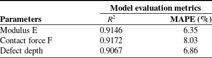
The results of model’s prediction are summarized in the following table:
From table II, it is evident that the model can accurately predict the parameters
 $E$
,
 $D$
, and
 $F$
. Consequently, the trained machine learning model serves as the “brain” of the tactile sensor, processing strain gauge signals and converting them into physical parameters such as elastic modulus and defect depth. This role underscores the sensor’s ability to function autonomously in real-time applications, where precise and efficient contact characteristic analysis is crucial.
The high accuracy of the machine learning model, combined with the integration of a fast-training LSTM network, capable of processing a given dataset in under 10 s, ensures that the sensor system can operate online with high precision and minimal processing time.
5. Conclusion
The study presents a new soft tactile sensor with a dome-shaped design that can dynamically adjust its stiffness by using pneumatic pressure to perform various sensing tasks, including accurately estimating the elastic modulus and the depths of the defects within soft materials. By integrating numerical simulations with machine learning techniques, the proposed system provides a comprehensive solution that minimizes the reliance on extensive physical experiments while maintaining high prediction accuracy. In this method, the numerical simulation data are synchronized with the experimental data to generate a robust training data set for the machine learning model. This approach not only improves predictive precision but also significantly reduces resource demands, including time, material costs, and the complexity of experimental setups.
The results indicate that the machine learning models utilized in this study exhibit strong performance in predicting contact forces, elastic modulus, and defect depths, with consistently low error rates. This high accuracy is further validated through scatter plots, residual plots, and visual comparison graphs, which confirm the reliability and robustness of the predictions.
Moreover, the study highlights the promising application of morphological computation in reducing system complexity while maintaining functionality. By eliminating the need for multiple sensor components, the proposed tactile sensor achieves a simplified design, data processing. Thus, morphological computation has significant potential in advancing the design, development of soft tactile sensors, and soft robotic systems.
The findings of this study highlight the sensor’s ability to detect variations in the elastic modulus and irregularities of the stiffness of the subsurface using soft synthetic materials. Since these materials exhibit mechanical properties similar to those of biological soft tissues, our results indicate the potential applicability of the sensor in medical diagnostics, such as tumor detection. Future research will focus on direct validation with biological tissue samples to further confirm and refine this application.
Furthermore, the findings of this study highlight the sensor’s ability to detect variations in the elastic modulus and irregularities in subsurface stiffness using soft synthetic materials. Since these materials exhibit mechanical properties similar to those of biological soft tissues, our results indicate the potential applicability of the sensor in medical diagnostics, such as tumor detection. Future research will focus on direct validation with biological tissue samples to further confirm and refine this application.
While the proposed sensor demonstrates high accuracy in controlled conditions, its sensitivity and adaptability to highly nonuniform or viscoelastic materials remain areas for future exploration. In this study, viscoelastic properties—although important for capturing time-dependent behaviors such as those occurring during sliding contact—were not included in our modeling and simulation. This choice was made because including viscoelastic effects would significantly increase the computational cost and simulation time, making it difficult to generate the large amount of data needed for training our sensor using the proposed method. Despite this, the model trained on both simulation and experimental data achieved high prediction accuracy, suggesting that the absence of viscoelasticity had little impact on the overall results and conclusions. Nevertheless, further improvements in sensor calibration and adaptive learning strategies could help improve performance when working with more complex soft materials, such as those with high viscosity or lower elastic modulus than the materials investigated in this study.
Besides, unlike human mechanoreceptors, which are highly sensitive to strain rate, the strain gauge used in this study primarily responds to absolute strain intensity. Although this provides a reliable measure of material properties, incorporating strain rate sensitivity would require different sensing elements and advanced machine learning models, such asRNNs or temporal convolutional networks, to process time-dependent signals. Future research will explore these approaches to further enhance the sensor’s ability to capture dynamic interactions and improve tactile perception in sliding motions.
Model evaluation metrics for different parameters.

Author contributions
Bui Manh Cuong and Hiep Xuan Trinh conceived, designed the study, and conducted data gathering. Mai Xuan Trang and Phan Viet Anh performed machine learning and statistical analyses. Hiep Xuan Trinh wrote the article.
Financial support
This research received no specific grant from any funding agency, commercial, or not-for-profit sectors.
Competing interests
The authors declare no conflicts of interest exist.
Ethical approval
Not applicable.