1. Introduction
In recent years, parallel mechanisms have demonstrated unique advantages in applications requiring high rigidity, precision, and load-bearing capacity, thanks to their high operational accuracy, high rigidity, strong load-bearing capacity, and excellent dynamic performance [Reference Xing, Ma, Tian and Zhang1], thereby playing a pivotal role [Reference Li, Qu, Kuang, Carbone and Guo2, Reference Wang, Xie and Liu3]. Currently, parallel mechanisms are widely used in numerous fields [Reference He, Duan, Qu and Xiao4], including minimally invasive surgical robots [Reference Lin, Guo and Cheng5], rehabilitation medical devices [Reference Jiang, Morita, Wang, Shinoda, Meng, Botta, Quaglia, Ceccarelli and Takeda6, Reference Diego, Macho, Campa, Herrero, Diez, Corral and Pinto7], industrial manufacturing [Reference Tao, Xu, Zhang and Tan8], aerospace [Reference Sun, Zhang, Wang and Chu9], and motion simulators [Reference Chen, Song, Li, Yan and Zhao10]. They have become an integral part of high-end manufacturing equipment and represent one of the core research areas in modern kinematics and robotics.
In practical applications of parallel mechanisms, many operating conditions require only 2–5 degrees of freedom to meet motion requirements, and therefore, parallel mechanisms with fewer degrees of freedom have gradually become a research focus in this field [Reference Zheng, Zhang and Li11]. Among these, extensive research has been conducted by many scholars [Reference Song, Kang and Dai12, Reference Gong and Lou13] on the kinematics, dynamics, and other aspects of three-degree-of-freedom parallel mechanisms with two rotational degrees of freedom (R) and one translational degree of freedom (T), as represented by the 3-RPS mechanism proposed by Hunt [Reference Hunt14] in 1983. Such mechanisms have found widespread application in many core engineering fields due to their simple structure and ease of control [Reference Chen, Kong, Zhao and Huang15, Reference Aldanmaz, Ayit, Kiper and Dede16]. Examples include high-precision machining centers for complex workpieces designed based on the 2PRU-PSR mechanism [Reference Xu, Ye and Li17], the Exechon Robot based on the 2UPR-SPR mechanism [Reference Shen, Yang, Wang and Dai18], as well as the 2URRR-URR [Reference Yaşır, Kiper and Dede19] and 2CRRR-CRR [Reference Lin, Guo and Cheng20] mechanisms used in minimally invasive surgery.
Common 2R1T parallel mechanisms typically employ a three-limb configuration, which offers advantages including structural simplicity and has found practical application in high-precision, light-to-medium load machining operations such as polishing, drilling, and milling [Reference Zhang, Yue, Wei, Li, Liao and Xu21]. However, as engineering applications continue to expand, traditional three-limb 2R1T mechanisms have gradually revealed limitations such as restricted load-bearing capacity and insufficient stiffness, making them unable to meet the demands of heavy-load operating conditions. Consequently, four-limb 2R1T parallel mechanisms have emerged. Four-limb 2R1T parallel mechanisms have the same number of actuators as their degrees of freedom and are neither redundantly actuated nor kinematically redundant [Reference Li, Zhang, Jin, Chen and Ye22]. Compared with similar three-limb parallel mechanisms, four-limb 2R1T parallel mechanisms, such as 2UPU-2SPR [Reference Zhang, Yue, Wei, Li, Liao and Xu21], 2RPU-UPR-RPR [Reference Ma, Xu, Xu, Wang, Yao and Zhao23], and 3PUS-PU [Reference Zhou, Li, Sun and Yi24], offer superior bending and torsional stiffness. Furthermore, their overall stiffness typically surpasses that of other three-limb parallel mechanisms, resulting in better load-bearing performance and greater load-carrying capacity, making them particularly advantageous in heavy-load machining and other applications [Reference Ma, Xu, Xu, Wang, Yao and Zhao23].
Kinematic analysis forms the core foundation of theoretical research on parallel mechanisms, and position analysis is the core and prerequisite of kinematic analysis. Due to the motion coupling relationships between the various branches of parallel mechanisms, deriving their exact kinematic solutions is relatively difficult and represents one of the major challenges in this field. For solving the exact position solutions of 2R1T parallel mechanisms, commonly used analytical methods include the closed-loop vector method. For example, Peng et al. [Reference Peng, Chen, Che, Cui and Jin25] employed the vector method to derive the forward and inverse position analytical solutions for the UPS-RPU-PU mechanism and completed the scale optimization of the mechanism. In addition, numerical iterative methods and analytical elimination methods are also frequently applied in this field. However, the aforementioned methods either focus on complex algebraic operations or rely on numerical iterative approximations, suffering from issues such as poor geometric intuitiveness and cumbersome solution processes. In particular, for four-limb 2R1T mechanisms, their multi-loop, strongly coupled constraint characteristics increase the complexity of solving for exact positions. Therefore, there is an urgent need to introduce a novel mathematical tool to develop a general, concise, and efficient method for position determination.
Conformal geometric algebra (CGA) [Reference Zhang, Zhu and Li26, Reference Wei, Zhu, Xing, Guan and Dai27] is an extension of geometric algebra into conformal space, naturally integrating mathematical tools such as vector algebra, complex numbers, quaternions, and exterior algebra within a unified framework. It can intrinsically represent fundamental geometric primitives including points, lines, planes, and spheres, as well as rigid-body transformations such as rotations and translations, in a unified multivector form. Its operations are coordinate-free, allowing geometric manipulations to be fully converted into algebraic computations with clear geometric and physical meaning. Since Hestenes and others laid the theoretical foundation [Reference Hestenes and Sobczyk28], CGA has been further developed by scholars such as Dorst, Lasenby, and Hitzer [Reference Dorst and Mann29–Reference Hitzer31] and has been widely applied in fields including computer vision and robot kinematics, becoming an important tool for the unified modeling of geometric constraints and rigid-body motions. In robot kinematics, CGA not only provides a concise and geometrically interpretable new approach for the inverse kinematics of serial robots but also exhibits good compatibility and potential for solving the highly nonlinear and strongly coupled forward kinematics of parallel mechanisms. For example, Zhu et al. [Reference Zhu, Wei, Zhang and Liao32] proposed a CGA-based geometric modeling approach for the forward kinematics of the 3-RPR planar parallel mechanism, which is computationally concise, effective, and geometrically meaningful. Zhao [Reference Zhao33] investigated the 3-RPS parallel mechanism and, using CGA, established a forward kinematic model applicable to all configurations, with a modeling process independent of the coordinate system.
However, there is currently a gap in the literature regarding the solution of forward kinematics for four-limb 2R1T parallel mechanisms using CGA. Based on this, this paper focuses on a type of four-limb 2R1T parallel mechanism composed of three coplanar limbs and a spatial limb, and introduces the CGA mathematical framework to perform forward kinematic analysis. Based on the geometric perpendicular relationship between the line connecting the relevant articulation points and the common plane of the three coplanar limbs, this class of mechanisms is divided into two subclasses for exploration, namely, mechanisms without perpendicular constraints (WoPC) and mechanisms with perpendicular constraints (WPC). Here, the term perpendicular constraint is used in a purely geometric sense, referring to the perpendicular relationship between the specified line and plane, without implying any force-based or mechanical property. This classification is not intended to provide an absolute definition of mechanisms, but rather to enable the selection of a more concise and effective forward kinematics solution for a specific mechanism configuration. In short, this is a preliminary analysis strategy for solving forward kinematics. It thus provides a clear basis for the differentiated design of subsequent CGA modeling approaches. Corresponding CGA forward kinematic solution methods are proposed for the two subclasses. The proposed methods fully integrate motion operators with geometric intersection operations, significantly simplifying the solution process by circumventing or reducing the need for variable elimination. These methods are not only concise and efficient but also highly generalizable. Subsequently, using the 2UPU-2SPR configurations I and II as examples, combined with numerical examples and 3D simulation verification, the correctness and effectiveness of the proposed methods are demonstrated.
2. Fundamentals of conformal geometric algebra
The core idea of CGA [Reference Zhu and Zhang34] is to embed three-dimensional Euclidean space into a five-dimensional Minkowski space. This embedding allows various conformal transformations in three-dimensional space (such as rotations and translations) to be uniformly represented as orthogonal transformations in the higher-dimensional space, all of which can be realized through unified algebraic operations using the rotors of geometric algebra. This mechanism fundamentally achieves the algebraization, coordinate-independence, and unification of geometric elements and geometric transformations.
In CGA, the basic operations between vectors include the inner product, outer product, and geometric product, and satisfy the relation
 \begin{equation} \boldsymbol{ab}=\boldsymbol{a}\cdot \boldsymbol{b}+\boldsymbol{a}\wedge \boldsymbol{b} \end{equation}
A five-dimensional conformal geometric space is spanned by five orthogonal basis vectors: {
 $\boldsymbol{e}_{1}$
,
 $\boldsymbol{e}_{2}$
,
 $\boldsymbol{e}_{3}$
,
 $\boldsymbol{e}_{+}$
,
 $\boldsymbol{e}_{-}$
}, where {
 $\boldsymbol{e}_{1}$
,
 $\boldsymbol{e}_{2}$
,
 $\boldsymbol{e}_{3}$
} correspond to the basis vectors of the Cartesian coordinate axes in three-dimensional Euclidean space. The inner product of any two distinct basis vectors among the five is zero, and they satisfy
 \begin{equation} \boldsymbol{e}_{i}\boldsymbol{e}_{j}=\begin{cases} 1\\ \boldsymbol{e}_{i}\wedge \boldsymbol{e}_{j} \end{cases} \begin{array}{l} \begin{array}{ll} &\quad i=j \end{array}\\ \begin{array}{ll} &\quad i\neq j \end{array} \end{array}\begin{array}{ll} \left(i=1,2,3\right) &\quad \end{array}\begin{array}{lll} &\quad {\boldsymbol{e}}_{+}^{2}=1\begin{array}{ll} \begin{array}{ll} &\quad \end{array} &\quad \begin{array}{ll} {\boldsymbol{e}}_{-}^{2}=-1 &\quad \end{array} \end{array} & \end{array} \end{equation}
For ease of geometric interpretation, two null vectors are typically introduced as new basis vectors:
 \begin{equation} \boldsymbol{e}_{0}=\dfrac{\boldsymbol{e}_{-}-\boldsymbol{e}_{+}}{2}\begin{array}{ll} &\quad \boldsymbol{e}_{\infty }=\boldsymbol{e}_{-}+\boldsymbol{e}_{+} \end{array} \end{equation}
The unit pseudoscalar is denoted by
 $\boldsymbol{I}_{C}$
.
 \begin{equation} \boldsymbol{I}_{C}=\boldsymbol{e}_{1}\boldsymbol{e}_{2}\boldsymbol{e}_{3}\boldsymbol{e}_{0}\boldsymbol{e}_{\infty } \end{equation}
The dual of any multivector
 $\boldsymbol{A}$
is
 \begin{equation} \boldsymbol{A}^{\ast }=\boldsymbol{A}{\boldsymbol{I}}_{C}^{-1}=-\boldsymbol{A}\boldsymbol{I}_{C} \end{equation}
2.1. Representation of basic geometric objects
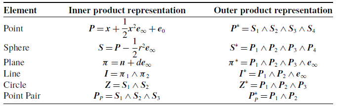
In CGA, basic geometric elements such as points, lines, planes, and spheres can be uniformly represented and directly manipulated through geometric operations. Geometric elements can be expressed in two ways: inner product notation and outer product notation. These two representations can be converted into one another via dual operations, as shown in Table I.
Algebraic representations of basic geometric elements in CGA.

Table I. Long description
The table compares inner and outer product representations of basic geometric elements. It includes six elements: Point, Sphere, Plane, Line, Circle, and Point Pair. For each element, the table provides two representations: Inner product representation and Outer product representation. The Point is represented as P equals x plus one half x squared e infinity plus e zero in inner product notation and as P star equals S 1 wedge S 2 wedge S 3 wedge S 4 in outer product notation. The Sphere is represented as S equals P minus one half r squared e infinity in inner product notation and as S star equals P 1 wedge P 2 wedge P 3 wedge P 4 in outer product notation. The Plane is represented as pi equals n plus d e infinity in inner product notation and as pi star equals P 1 wedge P 2 wedge P 3 wedge e infinity in outer product notation. The Line is represented as l equals pi 1 wedge pi 2 in inner product notation and as l star equals P 1 wedge P 2 wedge e infinity in outer product notation. The Circle is represented as Z equals S 1 wedge S 2 in inner product notation and as Z star equals P 1 wedge P 2 wedge P 3 in outer product notation. The Point Pair is represented as P P equals S 1 wedge S 2 wedge S 3 in inner product notation and as P star P equals P 1 wedge P 2 in outer product notation.
Given a point pair
 $\boldsymbol{P}_{P}$
, the two points composing this pair can be decomposed as
 \begin{align} \begin{array}{c} \boldsymbol{P}_{1,2}=\dfrac{\boldsymbol{T}_{b2}}{A_{\mathrm{var}}}\pm \dfrac{\sqrt{B_{\mathrm{var}}}}{A_{\mathrm{var}}}\boldsymbol{T}_{b1}\\[12pt] \begin{array}{llll} \boldsymbol{T}_{b1}=\boldsymbol{e}_{\infty }\cdot {\boldsymbol{P}}_{P}^{\ast } &\quad \boldsymbol{T}_{b2}=\boldsymbol{T}_{b1}\cdot {\boldsymbol{P}}_{P}^{\ast } &\quad A_{\mathrm{var}}=\boldsymbol{T}_{b1}\cdot \boldsymbol{T}_{b1} &\quad B_{\mathrm{var}}={\boldsymbol{P}}_{P}^{\ast }\cdot {\boldsymbol{P}}_{P}^{\ast } \end{array} \end{array} \end{align}
The relationship between the inner product of two points
 $\boldsymbol{P}_{1}$
and
 $\boldsymbol{P}_{2}$
their Euclidean distance
 $d_{12}$
is given by
 \begin{equation} \boldsymbol{P}_{1}\cdot \boldsymbol{P}_{2}=-\dfrac{1}{2}d_{12} \end{equation}
2.2. Expression of rigid body motion
The motion of a rigid body can be expressed as a combination of rotation and translation in three-dimensional space. In CGA, the rotation of a rigid body
 $\boldsymbol{O}$
is realized by the rotation operator
 $\boldsymbol{R}$
.
 \begin{equation} \boldsymbol{O}'=\boldsymbol{RO}\tilde{\boldsymbol{R}} \end{equation}
where
 $\tilde{\boldsymbol{R}}$
is the conjugate of
 $\boldsymbol{R}$
, and the rotation operator
 $\boldsymbol{R}$
can be expressed as
 \begin{equation} \boldsymbol{R}=\cos \left(\dfrac{\theta }{2}\right)-\sin \left(\dfrac{\theta }{2}\right)\boldsymbol{L} \end{equation}
where
 $\boldsymbol{L}$
denotes the unit bivector of the rotation plane, and
 $\theta$
is the angle of rotation.
In CGA, the translation of a rigid body
 $\boldsymbol{O}$
can be achieved using the translation operator
 $\boldsymbol{T}$
.
 \begin{equation} \boldsymbol{O}''=\boldsymbol{T}\boldsymbol{O }\tilde{\boldsymbol{T}} \end{equation}
where
 $\tilde{\boldsymbol{T}}$
is the conjugate of
 $\boldsymbol{T}$
, and the translation operator
 $\boldsymbol{T}$
can be expressed as
 \begin{equation} \boldsymbol{T}=1-\dfrac{1}{2}\boldsymbol{t}\boldsymbol{e}_{\infty } \end{equation}
where
 $\boldsymbol{t}$
is the three-dimensional translation vector.
The composition of multiple transformations corresponds to the geometric product of the corresponding rotors and is uniformly represented by the motion operator
 $\boldsymbol{M}$
. For example, the composition of rotation and translation corresponds to the motion operator.
 \begin{equation} \boldsymbol{M}=\boldsymbol{RT} \end{equation}
In CGA, the motion of a rigid body
 $\boldsymbol{O}$
can be uniformly realized via the motion operator
 $\boldsymbol{M}$
.
 \begin{equation} \boldsymbol{O}'''=\boldsymbol{MO}\tilde{\boldsymbol{M}} \end{equation}
where
 $\tilde{\boldsymbol{M}}$
is the conjugate of
 $\boldsymbol{M}$
.
3. Forward kinematic analysis of WoPC four-limb 2R1T parallel mechanisms
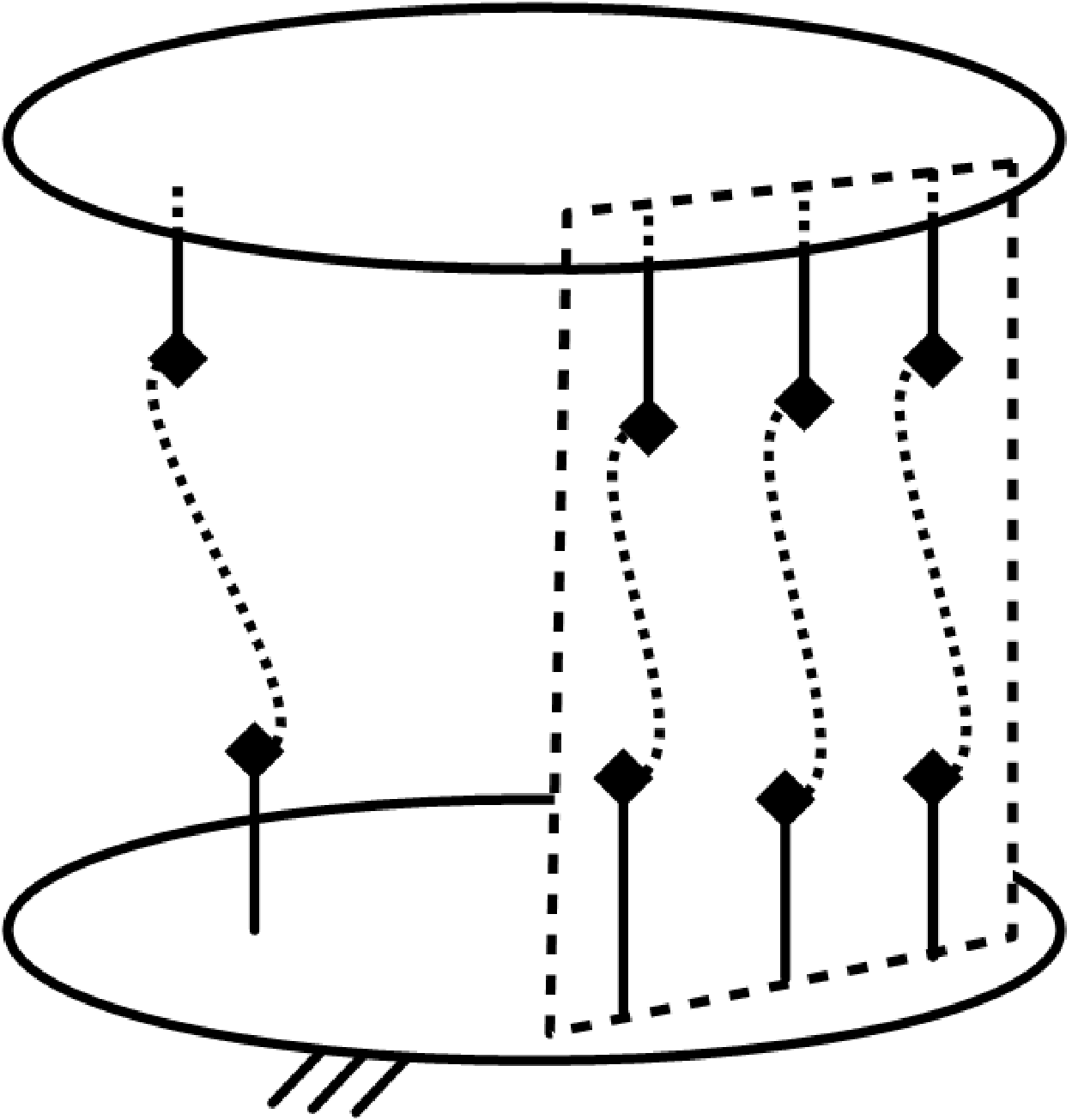
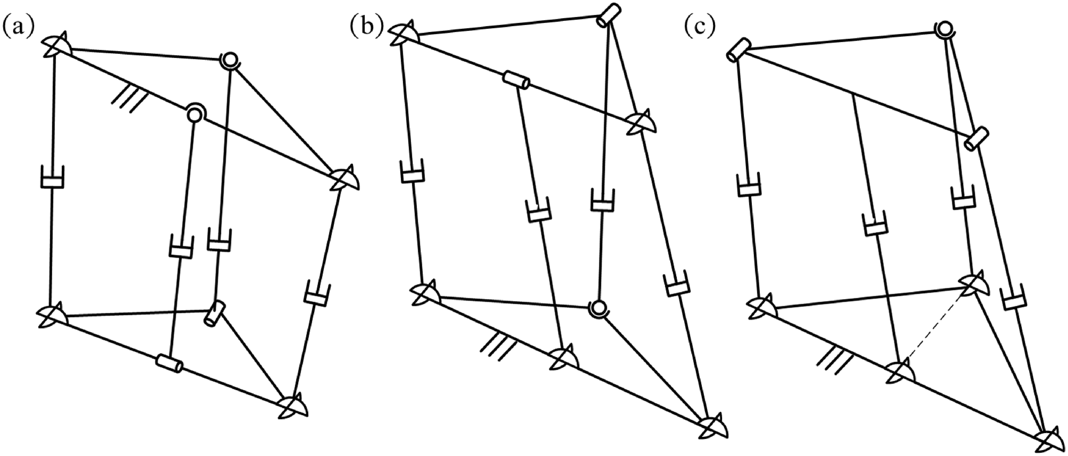
A common four-limb 2R1T parallel mechanism consisting of three coplanar limbs and one spatial limb is shown in Figure 1. Each of the two coplanar limbs and the one spatial limb in this type of mechanism contains a drive joint. Based on the geometric perpendicular relationship between the line connecting the moving-platform articulation points of the other coplanar limb and the spatial limb and the common plane of the three coplanar limbs, these mechanisms can be classified into two categories. In the first subclass of mechanisms, referred to as mechanisms WoPC, the aforementioned line has no fixed perpendicular relationship with the common plane of the three coplanar limbs. Furthermore, even after removing the articulation point between the spatial limb and the moving platform, this class of mechanisms still possesses complete constraint conditions, exhibiting a certain degree of constraint redundancy. Common examples of this class of mechanisms include the specific configurations of 2UPU-2SPR (Configuration I) [Reference Zhang, Yue, Wei, Li, Liao and Xu21], 2UPU-SPR-UPR [Reference Zhang, Yue, Wei and Li35], and 2UPR-UPS-UP [Reference Chen and Chen36], as shown in Figure 2.
Schematic diagram of the general structure of the 2R1T parallel mechanism with three coplanar limbs and one spatial limb.

Common WoPC 2R1T parallel mechanisms: (a) 2UPU-2SPR (Configuration I); (b) 2UPU-SPR-UPR; (c) 2UPR-UPS-UP.

3.1. CGA-based forward kinematic analysis of WoPC four-limb 2R1T parallel mechanisms
CGA unifies rigid-body motions and the intersections of geometric entities (such as planes and spheres) within a single mathematical framework. However, existing studies on the forward kinematic solutions of parallel mechanisms have primarily focused on utilizing the intersections of geometric elements [Reference Zhu, Wei, Zhang and Liao32], while neglecting the expression and role of motion operators within this framework. Only by reasonably integrating the two can solutions be derived more effectively. This paper proposes a unified solution method for the forward kinematics of WoPC four-limb 2R1T parallel mechanisms, based on CGA combined with motion operators and geometric intersections.
The core steps are as follows:
-
Step 1: Appropriate unknown parameters are set based on the unique geometric structure of this class of mechanisms.
-
Step 2: Motion operators are applied to derive the parametric expression of the first moving-platform vertex from the known CGA expressions of the fixed-platform vertices.
-
Step 3: Basic geometric entities such as planes are constructed, and the expressions of the remaining moving-platform vertices are derived via duality and intersection operations.
-
Step 4: Inner product operations are performed based on the geometric constraints within the mechanism to obtain a univariate high-order equation. Upon solving this equation, the parametric expressions of the moving-platform vertices are substituted back to determine the pose of the mechanism.
This approach circumvents the need for variable elimination throughout the entire process, rendering the solution procedure concise and efficient.
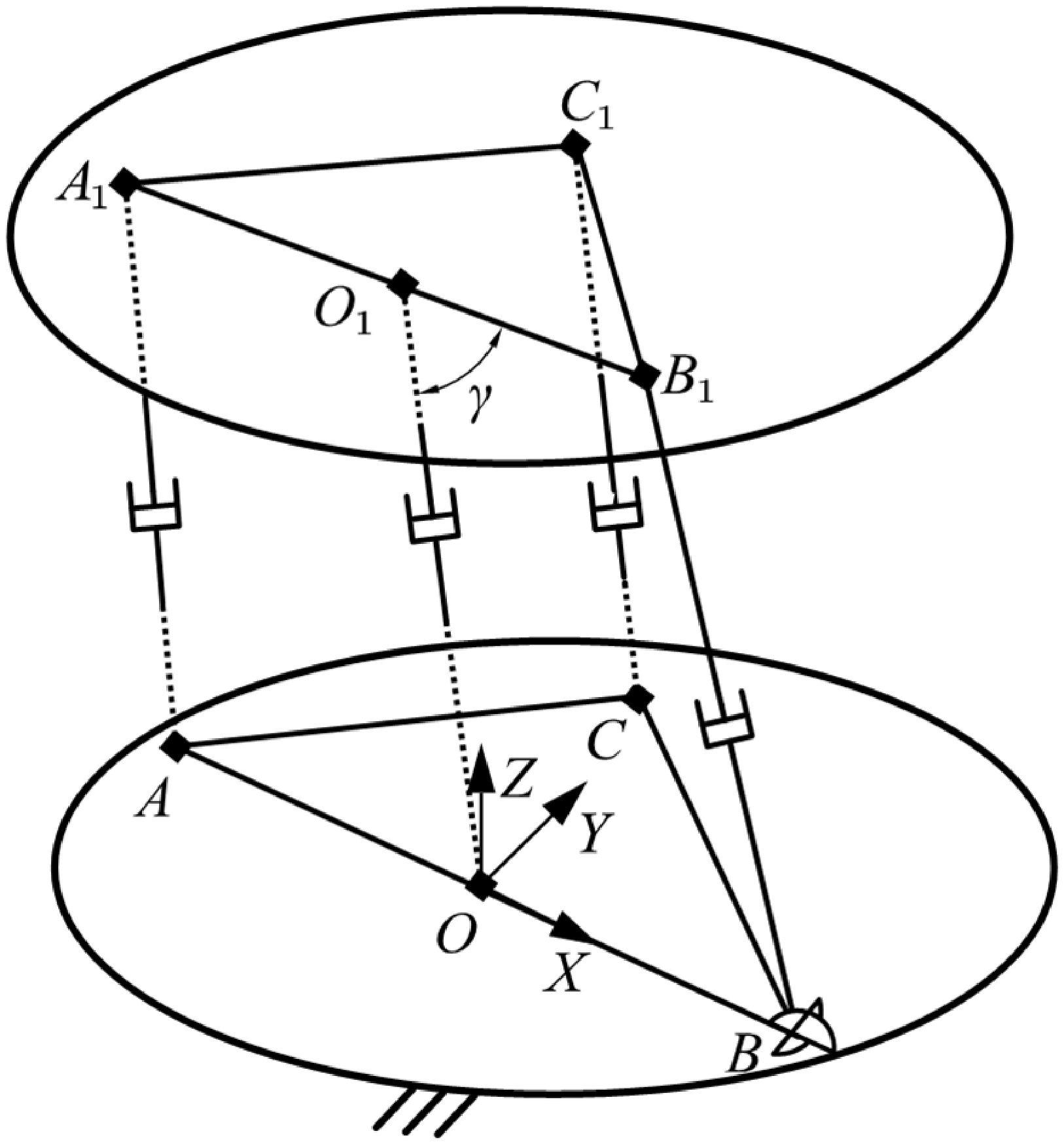
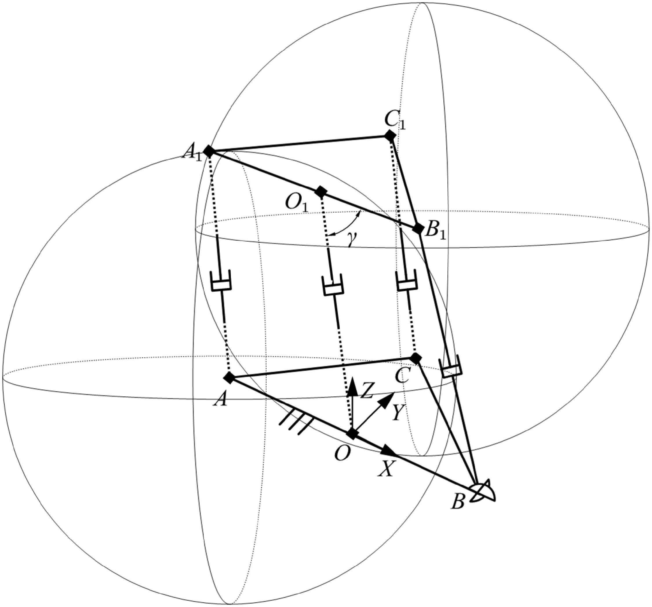
As shown in Figure 3, for this class of mechanisms, a fixed coordinate system is established with point
 $\boldsymbol{O}$
as the origin. The direction from
 $\boldsymbol{O}$
to
 $\boldsymbol{B}$
defines the
 $X$
-axis, and the direction perpendicular to the
 $X$
-axis and pointing toward point
 $\boldsymbol{C}$
defines the
 $Y$
-axis.
Schematic diagram of WoPC four-limb 2R1T parallel mechanisms.

Figure 3. Long description
A schematic diagram of a four-limb 2R1T parallel mechanism. The diagram shows two parallel planes with various labeled points and lines connecting them. The upper plane contains points labeled A1, B1, C1, and O1, while the lower plane contains points labeled A, B, C, and O. The points are connected by lines representing the limbs of the mechanism. The angle γ is marked between lines O1B1 and O1O1. The lower plane also includes a coordinate system with axes labeled X, Y, and Z. The diagram illustrates the spatial relationships and connections between the points in the parallel mechanism.
Based on the CGA representations of the points in Table I and the fundamental CGA operations, the conformal geometric expressions of the fixed-platform joints
 $\boldsymbol{A}$
,
 $\boldsymbol{B}$
,
 $\boldsymbol{C}$
, and
 $\boldsymbol{O}$
in the fixed coordinate system are given by
 \begin{equation} \begin{array}{l} \begin{array}{lll} \boldsymbol{A}=\boldsymbol{a}+\dfrac{1}{2}\boldsymbol{a}^{2}\boldsymbol{e}_{\infty }+\boldsymbol{e}_{0} & &\quad \boldsymbol{B}=\boldsymbol{b}+\dfrac{1}{2}\boldsymbol{b}^{2}\boldsymbol{e}_{\infty }+\boldsymbol{e}_{0} \end{array}\\[8pt] \begin{array}{lll} \boldsymbol{C}=\boldsymbol{c}+\dfrac{1}{2}\boldsymbol{c}^{2}\boldsymbol{e}_{\infty }+\boldsymbol{e}_{0} & &\quad \boldsymbol{O}=\boldsymbol{o}+\dfrac{1}{2}\boldsymbol{o}^{2}\boldsymbol{e}_{\infty }+\boldsymbol{e}_{0} \end{array} \end{array} \end{equation}
where
 $\boldsymbol{a}$
,
 $\boldsymbol{b}$
,
 $\boldsymbol{c}$
, and
 $\boldsymbol{o}$
denote point vectors in three-dimensional Euclidean space.
Suppose that the U-joint at
 $\boldsymbol{B}$
rotates by an angle
 $\alpha$
about an axis parallel to the
 $X$
-axis, and subsequently by an angle
 $\beta$
about its second axis; the motion from point
 $\boldsymbol{O}$
to
 $\boldsymbol{B}_{1}$
can then be realized by a motion operator.
 \begin{equation} {}^{O}{\boldsymbol{M}}{_{B1}^{}}=\boldsymbol{T}_{X}\boldsymbol{R}_{X}\boldsymbol{R}_{1Y}\boldsymbol{T}_{1X} \end{equation}
 \begin{equation} \boldsymbol{T}_{X}=1-\dfrac{d_{OB}}{2}\boldsymbol{e}_{1}\boldsymbol{e}_{\infty } \end{equation}
 \begin{equation} \boldsymbol{R}_{X}=\cos \left(\dfrac{\alpha }{2}\right)-\sin \left(\dfrac{\alpha }{2}\right)\boldsymbol{e}_{23} \end{equation}
 \begin{equation} \boldsymbol{R}_{1Y}=\cos \left(\dfrac{\beta }{2}\right)-\sin \left(\dfrac{\beta }{2}\right)\boldsymbol{e}_{31} \end{equation}
 \begin{equation} \boldsymbol{T}_{1X}=1-\dfrac{d_{B{B_{1}}}}{2}\boldsymbol{e}_{1}\boldsymbol{e}_{\infty } \end{equation}
 $\boldsymbol{B}_{1}$
can be expressed as follows:
 \begin{equation} \boldsymbol{B}_{1}=\left({}^{O}{\boldsymbol{M}}{_{B1}^{}}\right)\boldsymbol{O}\left({}^{O}{\tilde{\boldsymbol{M}}}{_{B1}^{}}\right) \end{equation}
As shown in Figure 4, point
 $\boldsymbol{A}_{1}$
lies simultaneously on spherical surface
 $\boldsymbol{S}_{{AA_{1}}}$
(centered at
 $\boldsymbol{A}$
with radius
 $d_{{AA_{1}}}$
) and spherical surface
 $\boldsymbol{S}_{{{B_{1}}A_{1}}}$
(centered at
 $\boldsymbol{B}_{1}$
with radius
 $d_{{A_{1}}{B_{1}}}$
). Furthermore, points
 $\boldsymbol{A}$
,
 $\boldsymbol{A}_{1}$
,
 $\boldsymbol{B}_{1}$
, and
 $\boldsymbol{B}$
are coplanar within plane
 $\boldsymbol{\pi }$
. Therefore, the point pair
 ${\boldsymbol{P}_{PA}}_{1}$
corresponding to point
 $\boldsymbol{A}_{1}$
can be determined by the outer product of the three surfaces.
 \begin{equation} \boldsymbol{P}_{P{A_{1}}}=\boldsymbol{S}_{A{A_{1}}}\wedge \boldsymbol{S}_{{B_{1}}{A_{1}}}\wedge \boldsymbol{\pi } \end{equation}
Schematic diagram of the solution for point
 $\boldsymbol{A}_{1}$
.

Based on the fundamental expressions of planes given in Table I, the dual representation of the plane
 $\boldsymbol{\pi }$
can be readily obtained.
 \begin{equation} \boldsymbol{\pi }^{\ast }=\boldsymbol{B}_{1}\wedge \boldsymbol{B}\wedge \boldsymbol{C}\wedge \boldsymbol{e}_{\infty } \end{equation}
Combining Eq. (5) and Eq. (22) yields the conformal geometric expression of plane
 $\boldsymbol{\pi }$
.
 \begin{equation} \boldsymbol{\pi }=\boldsymbol{\pi }^{\ast }{\boldsymbol{I}}_{C}^{-1} \end{equation}
Combining the basic expression of a sphere in Table I readily yields the conformal geometric expressions of sphere
 $\boldsymbol{S}_{{AA_{1}}}$
and sphere
 $\boldsymbol{S}_{{{B_{1}}A_{1}}}$
.
 \begin{equation} \boldsymbol{S}_{A{A_{1}}}=\boldsymbol{A}-\dfrac{1}{2}{d}_{AA_{1}}^{2}\boldsymbol{e}_{\infty } \end{equation}
 \begin{equation} \boldsymbol{S}_{{B_{1}}{A_{1}}}=\boldsymbol{B}_{1}-\dfrac{1}{2}{d}_{A_{1}B_{1}}^{2}\boldsymbol{e}_{\infty } \end{equation}
Combining Eqs. (5) and (22) yields the dual vector representation of point pair
 ${\boldsymbol{P}_{PA}}_{1}$
.
 \begin{equation} {\boldsymbol{P}}_{PA_{1}}^{\ast }=\boldsymbol{P}_{P{A_{1}}}{\boldsymbol{I}}_{C}^{-1} \end{equation}
From the point pair extraction formula (6) and Eq. (26),
 $\boldsymbol{A}_{1}$
can be obtained.
 \begin{equation} \begin{array}{c} \boldsymbol{A}_{1}=\dfrac{\boldsymbol{T}_{a1b2}}{A_{a1\mathrm{var}}}+\dfrac{K_{A}\sqrt{B_{a1\mathrm{var}}}}{A_{a1\mathrm{var}}}\boldsymbol{T}_{a1b1}\\[8pt] \begin{array}{lll} \boldsymbol{T}_{a1b1}=\boldsymbol{e}_{\infty }\cdot {\boldsymbol{P}}_{PA_{1}}^{\ast } & \boldsymbol{T}_{a1b2}=\boldsymbol{T}_{a1b1}\cdot {\boldsymbol{P}}_{PA_{1}}^{\ast } & A_{a1\mathrm{var}}=\boldsymbol{T}_{a1b1}\cdot \boldsymbol{T}_{a1b1} \end{array}\\[8pt] \begin{array}{ll} B_{a1\mathrm{var}}={\boldsymbol{P}}_{PA_{1}}^{\ast }\cdot {\boldsymbol{P}}_{PA_{1}}^{\ast } & K_{A}=\pm 1 \end{array} \end{array} \end{equation}
Given that
 $\boldsymbol{O}_{1}$
is located between
 $\boldsymbol{A}_{1}$
and
 $\boldsymbol{B}_{1}$
, it follows that:
 \begin{equation} \boldsymbol{O}_{1}=\dfrac{d_{{O_{1}}{B_{1}}}\boldsymbol{A}_{1}+d_{{O_{1}}{A_{1}}}\boldsymbol{B}_{1}}{d_{{A_{1}}{B_{1}}}}-\dfrac{d_{{O_{1}}{B_{1}}}d_{{O_{1}}{A_{1}}}}{2}\boldsymbol{e}_{\infty } \end{equation}
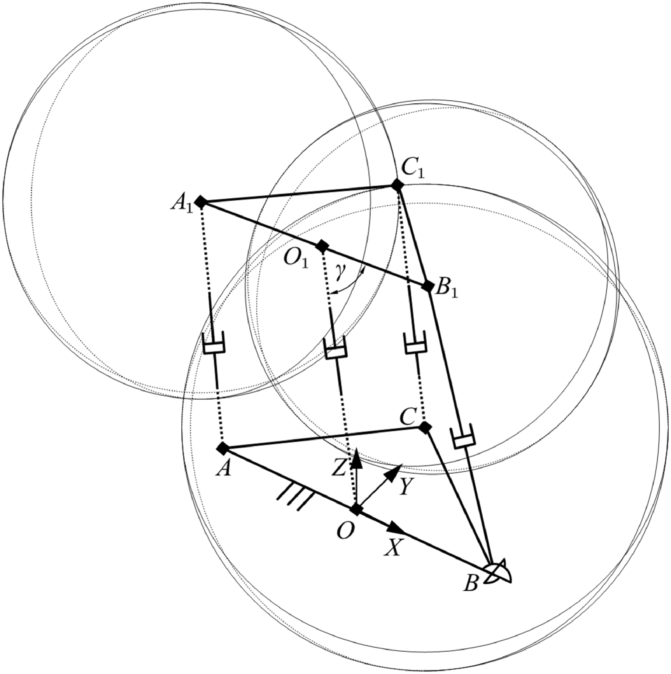
As shown in Figure 5, point
 $\boldsymbol{C}_{1}$
lies simultaneously on three spherical surfaces: sphere
 $\boldsymbol{S}_{{CC_{1}}}$
(centered at
 $\boldsymbol{C}$
with radius
 $d_{{CC_{1}}}$
), sphere
 $\boldsymbol{S}_{{{B_{1}}C_{1}}}$
(centered at
 $\boldsymbol{B}_{1}$
with radius
 $d_{{{B_{1}}C_{1}}}$
), and sphere
 $\boldsymbol{S}_{{{A_{1}}C_{1}}}$
(centered at
 $\boldsymbol{A}_{1}$
with radius
 $d_{{{A_{1}}C_{1}}}$
). Therefore, the point pair
 ${\boldsymbol{P}_{PC}}_{1}$
corresponding to point
 $\boldsymbol{C}_{1}$
can be determined by the outer product of these three spheres.
 \begin{equation} \boldsymbol{P}_{P{C_{1}}}=\boldsymbol{S}_{C{C_{1}}}\wedge \boldsymbol{S}_{{A_{1}}{C_{1}}}\wedge \boldsymbol{S}_{{B_{1}}{C_{1}}} \end{equation}
Combining the basic expression of a sphere in Table I readily yields the conformal geometric expressions of sphere
 $\boldsymbol{S}_{{CC_{1}}}$
, sphere
 $\boldsymbol{S}_{{{A_{1}}C_{1}}}$
and sphere
 $\boldsymbol{S}_{{{B_{1}}C_{1}}}$
.
 \begin{equation} \boldsymbol{S}_{C{C_{1}}}=\boldsymbol{C}-\dfrac{1}{2}{d}_{CC_{1}}^{2}\boldsymbol{e}_{\infty } \end{equation}
 \begin{equation} \boldsymbol{S}_{{A_{1}}{C_{1}}}=\boldsymbol{A}_{1}-\dfrac{1}{2}{d}_{A_{1}C_{1}}^{2}\boldsymbol{e}_{\infty } \end{equation}
 \begin{equation} \boldsymbol{S}_{{B_{1}}{C_{1}}}=\boldsymbol{B}_{1}-\dfrac{1}{2}{d}_{B_{1}C_{1}}^{2}\boldsymbol{e}_{\infty } \end{equation}
.
Schematic diagram of the solution for point
 $\boldsymbol{C}_{1}$
.

Figure 5. Long description
A diagram of a parallel mechanism showing geometric relationships and components. The diagram includes points labeled A, A1, B, B1, C, C1, O, O1, X, Y, and Z. Lines connect these points, indicating geometric relationships and distances. Right-angle symbols are present at several points, indicating perpendicular relationships. Circles and arcs represent paths or loci of certain points. The diagram illustrates the spatial arrangement and interactions within the parallel mechanism.
Combining Eqs. (5) and (29) yields the dual vector representation of point pair
 ${\boldsymbol{P}_{PC}}_{1}$
.
 \begin{equation} {\boldsymbol{P}}_{PC_{1}}^{\ast }=\boldsymbol{P}_{P{C_{1}}}{\boldsymbol{I}}_{C}^{-1} \end{equation}
From the point pair extraction formula (6) and Eq. (33),
 $\boldsymbol{C}_{1}$
can be obtained.
 \begin{equation} \begin{array}{c} \boldsymbol{C}_{1}=\dfrac{\boldsymbol{T}_{c1b2}}{A_{c1\mathrm{var}}}+\dfrac{K_{C}\sqrt{B_{c1\mathrm{var}}}}{A_{c1\mathrm{var}}}\boldsymbol{T}_{c1b1}\\[8pt] \begin{array}{lll} \boldsymbol{T}_{c1b1}=\boldsymbol{e}_{\infty }\cdot {\boldsymbol{P}}_{PC_{1}}^{\ast } &\quad \boldsymbol{T}_{c1b2}=\boldsymbol{T}_{c1b1}\cdot {\boldsymbol{P}}_{PC_{1}}^{\ast } &\quad A_{c1\mathrm{var}}=\boldsymbol{T}_{c1b1}\cdot \boldsymbol{T}_{c1b1} \end{array}\\[8pt] \begin{array}{ll} B_{c1\mathrm{var}}={\boldsymbol{P}}_{PC_{1}}^{\ast }\cdot {\boldsymbol{P}}_{PC_{1}}^{\ast } &\quad K_{C}=\pm 1 \end{array} \end{array} \end{equation}
At this point, Step 3 has been completed. Subsequently, only inner product operations based on the geometric constraint relations are required to obtain a univariate high-order equation, which is then solved.
For this class of mechanisms, the governing equation can be established by utilizing the relationship between
 $d_{{OA_{1}}}$
and
 $d_{{OB_{1}}}$
, together with the distance constraint satisfied by
 $d_{{{O_{1}}C_{1}}}$
. Within triangle
 $OA_{1}B_{1}$
, point
 $O_{1}$
lies on side
 $A_{1}B_{1}$
, and the segment
 $OO_{1}$
maintains a fixed angle with side
 $A_{1}B_{1}$
. Consequently, a distance equation exists between
 $d_{{OA_{1}}}$
and
 $d_{{OB_{1}}}$
that depends exclusively on a single unknown variable
 $\beta$
. By applying a half-angle trigonometric substitution to this variable, the expression reduces directly to a univariate polynomial equation. Subsequently, an equation based on the distance constraint satisfied by
 $d_{{O_{1}}C}$
is formulated, yielding a univariate polynomial equation in
 $\alpha$
. Solving this equation produces the corresponding value pairs {
 $\alpha$
,
 $\beta$
}. Finally, substituting these results back into the parametric expressions of the moving platform vertices fully determines the pose of the mechanism. The entire procedure requires no variable elimination, rendering the solution process both concise and efficient.
3.2. Forward kinematic analysis of a representative WoPC mechanism
Taking Configuration I of the 2UPU-2SPR parallel mechanism as an example, the feasibility and effectiveness of the forward kinematic solution approach proposed above are derived and verified.
As shown in Figure 6, the mechanism features two UPU limbs and two SPR limbs connecting the fixed platform and the moving platform. The R-joint axes of the two SPR limbs intersect perpendicularly. The R-joint axis at point
 $\boldsymbol{O}_{1}$
is collinear with segment
 $\boldsymbol{A}_{1}\boldsymbol{B}_{1}$
. Points
 $\boldsymbol{O}$
and
 $\boldsymbol{O}_{1}$
are the midpoints of
 $\boldsymbol{A}$
and
 $\boldsymbol{B}$
, and
 $\boldsymbol{A}_{1}$
and
 $\boldsymbol{B}_{1}$
, respectively. The lines connecting the attachment points of the four limbs to the fixed and moving platforms form two isosceles triangles, where
 $d_{AC} = d_{BC}$
and
 $d_{{{A_{1}}C_{1}}} = d_{{{B_{1}}C_{1}}}$
.
Schematic diagram of the 2UPU-2SPR (Configuration I).

The forward kinematic problem of this mechanism involves determining the output pose of the moving platform given its structural parameters and the input link lengths. The structural parameters
 $m$
,
 $n$
,
 $m_{1}$
, and
 $n_{1}$
correspond to
 $d_{OA}$
,
 $d_{OC}$
,
 $d_{{{O_{1}}A_{1}}}$
, and
 $d_{{{O_{1}}C_{1}}}$
, respectively, while the input quantities
 $L_{1}$
,
 $L_{2}$
, and
 $L_{3}$
represent the lengths of
 $d_{{AA_{1}}}$
,
 $d_{{BB_{1}}}$
, and
 $d_{{CC_{1}}}$
, respectively.
Substituting
 $m$
,
 $n$
,
 $m_{1}$
,
 $n_{1}$
,
 $L_{1}$
,
 $L_{2}$
, and
 $L_{3}$
into Eqs. (14), (20), (27), (28), and (34) yields the CGA expressions for all vertices of the fixed and moving platforms.
Based on the geometric characteristics of this mechanism, as illustrated in Figure 6, within triangle
 $OA_{1}B_{1}$
,
 $OO_{1}$
is the perpendicular bisector of
 $A_{1}B_{1}$
, and
 $d_{{OA_{1}}}$
equals
 $d_{{OB_{1}}}$
, from which we obtain:
 \begin{equation} \boldsymbol{A}_{1}\cdot \boldsymbol{O}-\boldsymbol{B}_{1}\cdot \boldsymbol{O}=0 \end{equation}
Substituting Eqs. (14), (20), and (27) into Eq. (35) yields, after simplification, the following:
 \begin{equation} {a}_{1x}^{2}+{a}_{1y}^{2}+{a}_{1z}^{2}-{b}_{1x}^{2}-{b}_{1y}^{2}-{b}_{1z}^{2}=0 \end{equation}
In the above expression, {
 $a_{1x}$
,
 $a_{1y}$
,
 $a_{1z}$
,
 $b_{1x}$
,
 $b_{1y}$
,
 $b_{1z}$
} are the components of
 $\boldsymbol{A}_{1}$
and
 $\boldsymbol{B}_{1}$
with respect to the vectors {
 $\boldsymbol{e}_{1}$
,
 $\boldsymbol{e}_{2}$
,
 $\boldsymbol{e}_{3}$
}, respectively.
For notational simplicity,
 $\cos (\theta )$
,
 $\sin (\theta )$
, and
 $\mathrm{t}an(\theta )$
are uniformly denoted as
 $c\theta$
,
 $s\theta$
, and
 $t\theta$
, respectively. Expanding and simplifying Eq. (36) yields:
 \begin{equation} \sum\limits_{i=0}^{2}f_{i}\left(c\beta \right)^{i}\pm \sqrt{\sum\limits_{j=0}^{4}f_{j+3}\left(c\beta \right)^{i}}=0 \end{equation}
In the above expression, the coefficients
 $f_{i}$
are all determined by the structural and input parameters. Equation (37) contains only a single unknown. Letting
 $x=t(\beta /2)$
, it follows readily from the half-angle trigonometric formula that
 $c\beta =(1-x^{2})/(1+x^{2})$
. Substituting this relation into Eq. (37), followed by transposition, squaring, and simplification, yields:
 \begin{equation} \sum\limits_{i=0}^{8}h_{i}x^{i}=0 \end{equation}
In the above expression, the coefficient
 $h_{i}$
is fully determined by
 $m$
,
 $m_{1}$
,
 $L_{1}$
, and
 $L_{2}$
.
Furthermore, since the direction of the R-joint axis at
 $\boldsymbol{C}_{1}$
coincides with
 $\boldsymbol{O}_{1}\boldsymbol{C}_{1}$
, it follows that
 $\boldsymbol{CC}_{1}$
is perpendicular to
 $\boldsymbol{O}_{1}\boldsymbol{C}_{1}$
. Combined with the distance formula, it is readily seen that:
 \begin{equation} {d}_{O_{1}C}^{2}=-2\boldsymbol{O}_{1}\cdot \boldsymbol{C} \end{equation}
 \begin{equation} {d}_{O_{1}C}^{2}-{d}_{CC_{1}}^{2}-{d}_{O_{1}C_{1}}^{2}=0 \end{equation}
Substituting Eqs. (14), (28), and (39) into Eq. (40) yields, after straightforward manipulation:
 \begin{equation} f_{11}+f_{12}s\alpha =0 \end{equation}
In the above expression, the coefficients are determined by the structural parameters, input parameters,
 $K_{A}$
, and
 $\beta$
. Letting
 $x_{1}=t(\alpha /2)$
, it follows readily from the half-angle trigonometric formula that
 $s\alpha =(2x_{1})/(1+{x}_{1}^{2})$
. Substituting this relation into Eq. (41) reduces the equation to:
 \begin{equation} \sum\limits_{i=0}^{2}j_{i}{x}_{1}^{i}=0 \end{equation}
In the above expression, the coefficient
 $j_{i}$
is fully determined by
 $m$
,
 $n$
,
 $m_{1}$
,
 $n_{1}$
,
 $L_{1}$
,
 $L_{2}$
, and
 $L_{3}$
.
Equation (38) is an 8th-degree univariate polynomial in terms of
 $x$
, while Eq. (42) is a quadratic univariate polynomial in terms of
 $x_{1}$
. Solving Eq. (38) yields
 $x$
, from which
 $\beta$
is then obtained via the half-angle trigonometric formula. Substituting
 $\beta$
back into Eqs. (37) and (42) yields the corresponding
 $x_{1}$
values, ultimately producing the solution set {
 $\alpha$
,
 $\beta$
}. Substituting these into Eqs. (20), (27), (28), and (34) gives the expressions for the principal vertices
 $\boldsymbol{B}_{1}$
,
 $\boldsymbol{A}_{1}$
,
 $\boldsymbol{O}_{1}$
, and
 $\boldsymbol{C}_{1}$
of the moving platform. Extracting the components of the vectors {
 $\boldsymbol{e}_{1}$
,
 $\boldsymbol{e}_{2}$
,
 $\boldsymbol{e}_{3}$
} provides the three-dimensional position coordinates of each point relative to the fixed coordinate system.
Similarly, for the 2UPU-SPR-UPR mechanism shown in Figure 2b, the geometric constraint conditions in Step 4 are completely consistent with those of the present mechanism. For the 2UPR-UPS-UP mechanism shown in Figure 2c, the geometric constraint in Step 4 involves a relationship between
 $d_{{OA_{1}}}$
and
 $d_{{OB_{1}}}$
, where
 $d_{{OC_{1}}}$
can be determined within triangle
 $OO_{1}C$
using the law of cosines. In both cases, a univariate polynomial equation is ultimately obtained without any variable elimination procedure. Due to space limitations, these derivations are not elaborated further here.
4. Forward kinematic analysis of WPC four-limb 2R1T parallel mechanisms
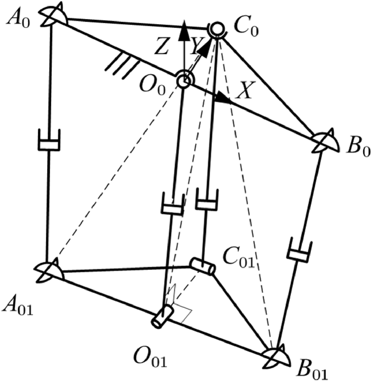
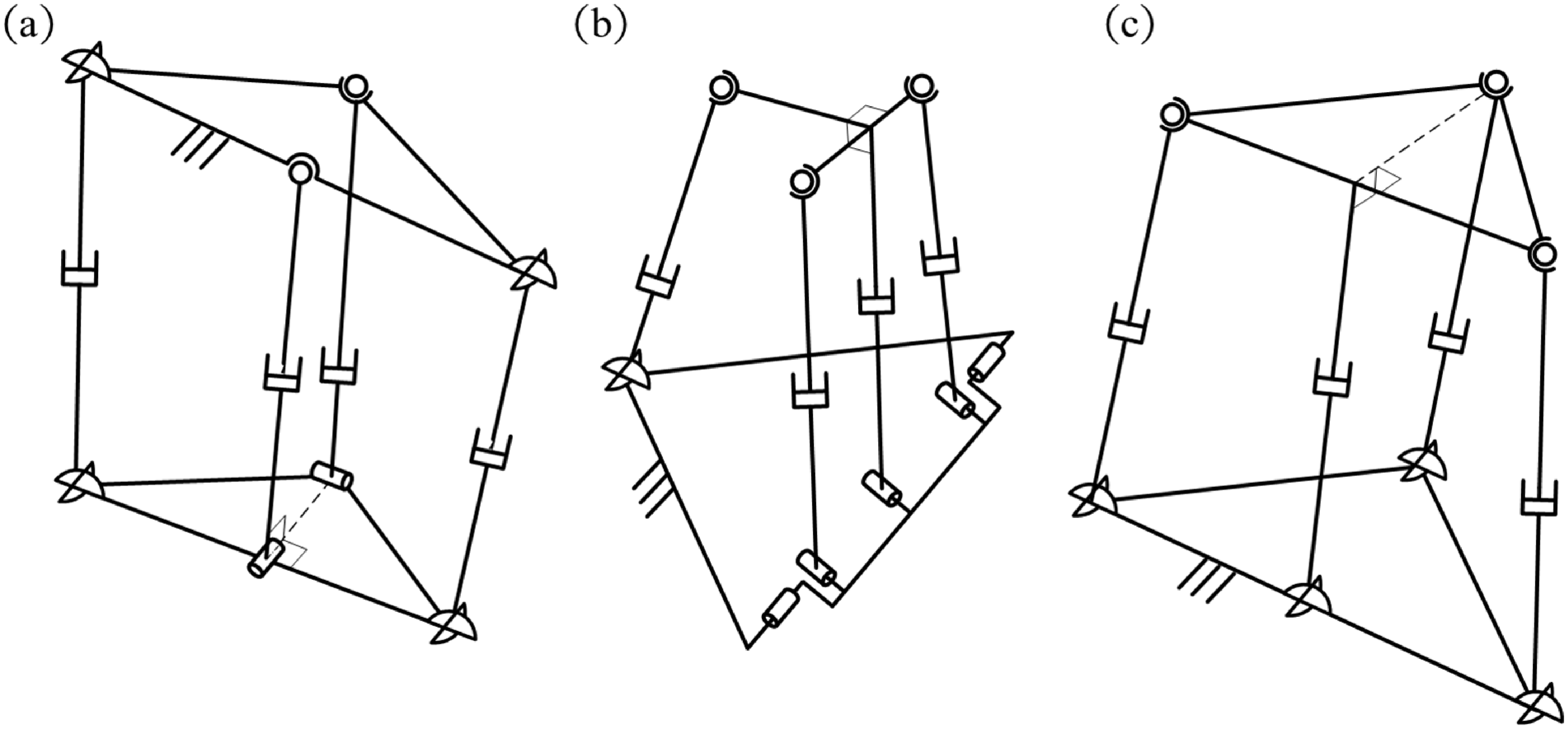
Among common four-limb 2R1T parallel mechanisms consisting of three coplanar limbs and one spatial limb, there exists a subclass, referred to as mechanisms WPC, in which the line connecting the moving-platform articulation points of the passive coplanar limb and the spatial limb consistently maintains a fixed perpendicular relationship with the common plane of the three coplanar limbs. This geometric perpendicular relationship is inherent to the mechanism’s architecture and is independent of the mechanism’s pose. Representative examples of this subclass include the specific configurations of 2UPU-2SPR (Configuration II) [Reference Zhang, Yue, Wei, Li, Liao and Xu21], R(2-RPS&RP)UPS [Reference Han, Shan, Liu, Xiao and Huang37, Reference Dong38], and 3UPS-UP [Reference Ma, Xu, Xu, Wang, Yao and Zhao23], as shown in Figure 7.
Common WPC 2R1T parallel mechanisms: (a) 2UPU-2SPR (Configuration II); (b) R(2-RPS&RP)UPS; (c) 3UPS-UP.

Figure 7. Long description
Panel A: Diagram of the 2UPU-2SPR parallel mechanism. It features circular nodes connected by lines, representing joints and links. The mechanism includes various symbols indicating different types of joints and connections. Panel B: Diagram of the R(2-RPS&RP)UPS parallel mechanism. Similar to Panel A, it shows circular nodes connected by lines, with specific symbols denoting different joint types and connections. Panel C: Diagram of the 3UPS-UP parallel mechanism. This diagram also features circular nodes connected by lines, with symbols representing various joints and connections.
4.1. CGA-based forward kinematic analysis of WPC four-limb 2R1T parallel mechanisms
The core steps of the unified solution approach for the forward kinematics of WPC four-limb 2R1T parallel mechanisms, which judiciously integrates motion operators and geometric intersections within the framework of CGA, are as follows:
-
Step 1: Based on the unique geometric structure of this class of mechanisms, appropriate unknown parameters are introduced.
-
Step 2: Using the CGA expressions of the known vertices together with the unknown parameters, the explicit expression of the first moving-platform vertex is obtained via motion operators.
-
Step 3: A set of fundamental geometric entities in CGA are constructed from the CGA expressions of the known vertices and the inherent geometric relations of the mechanism. The expressions of the remaining moving-platform vertices are then derived through a combined application of geometric intersection operations, duality operations, and motion operators.
-
Step 4: Inner-product equations are formulated based on the link-length constraints of the spatial limb.
-
Step 5: Additional inner-product operations are performed according to other geometric constraints within the mechanism. During this process, variable elimination may be required and can be straightforwardly accomplished using the resultant elimination method. This ultimately yields a univariate high-order equation. Solving this equation and substituting the result back into the parametric expressions of the moving-platform vertices fully determines the pose of the mechanism.
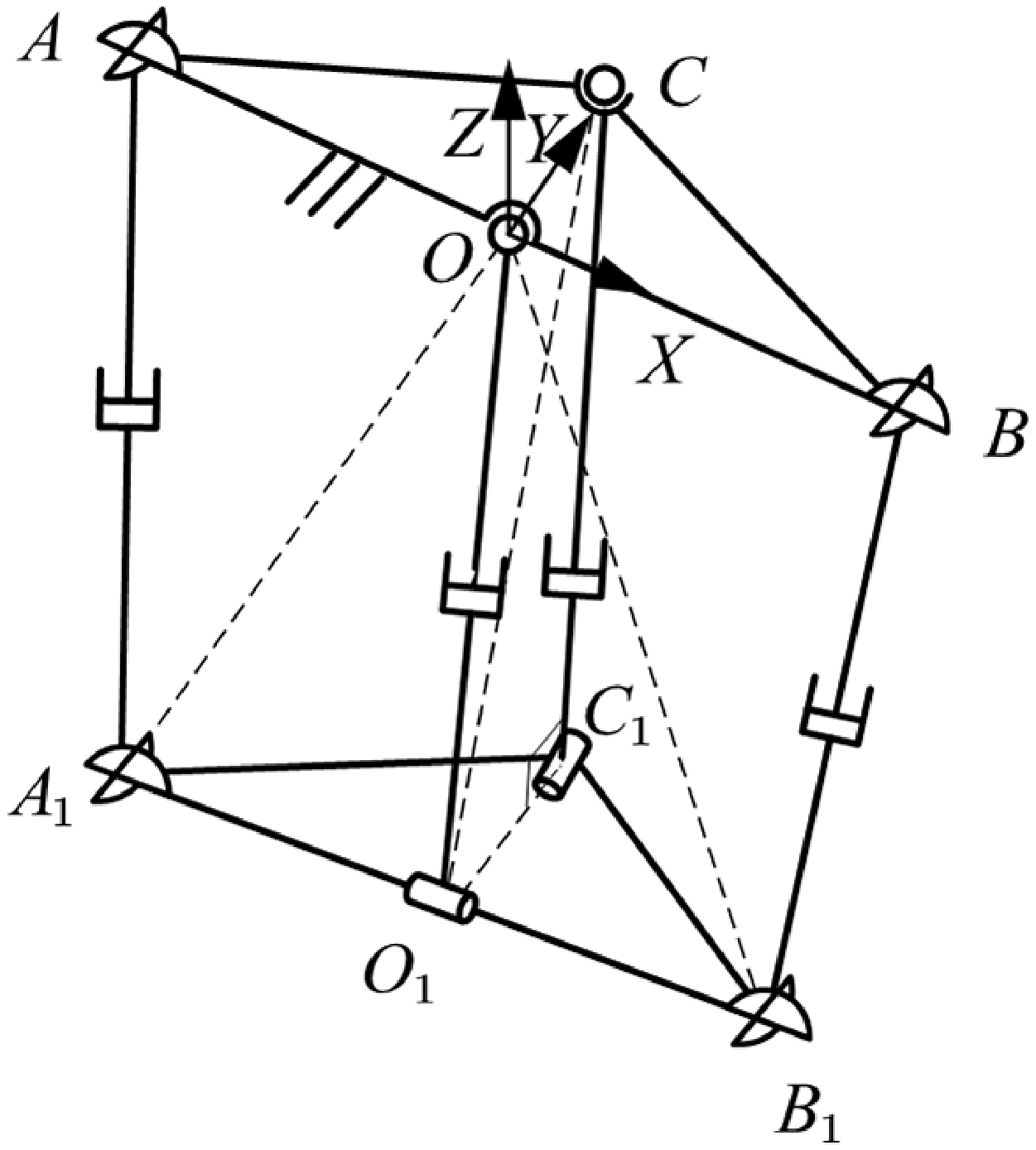
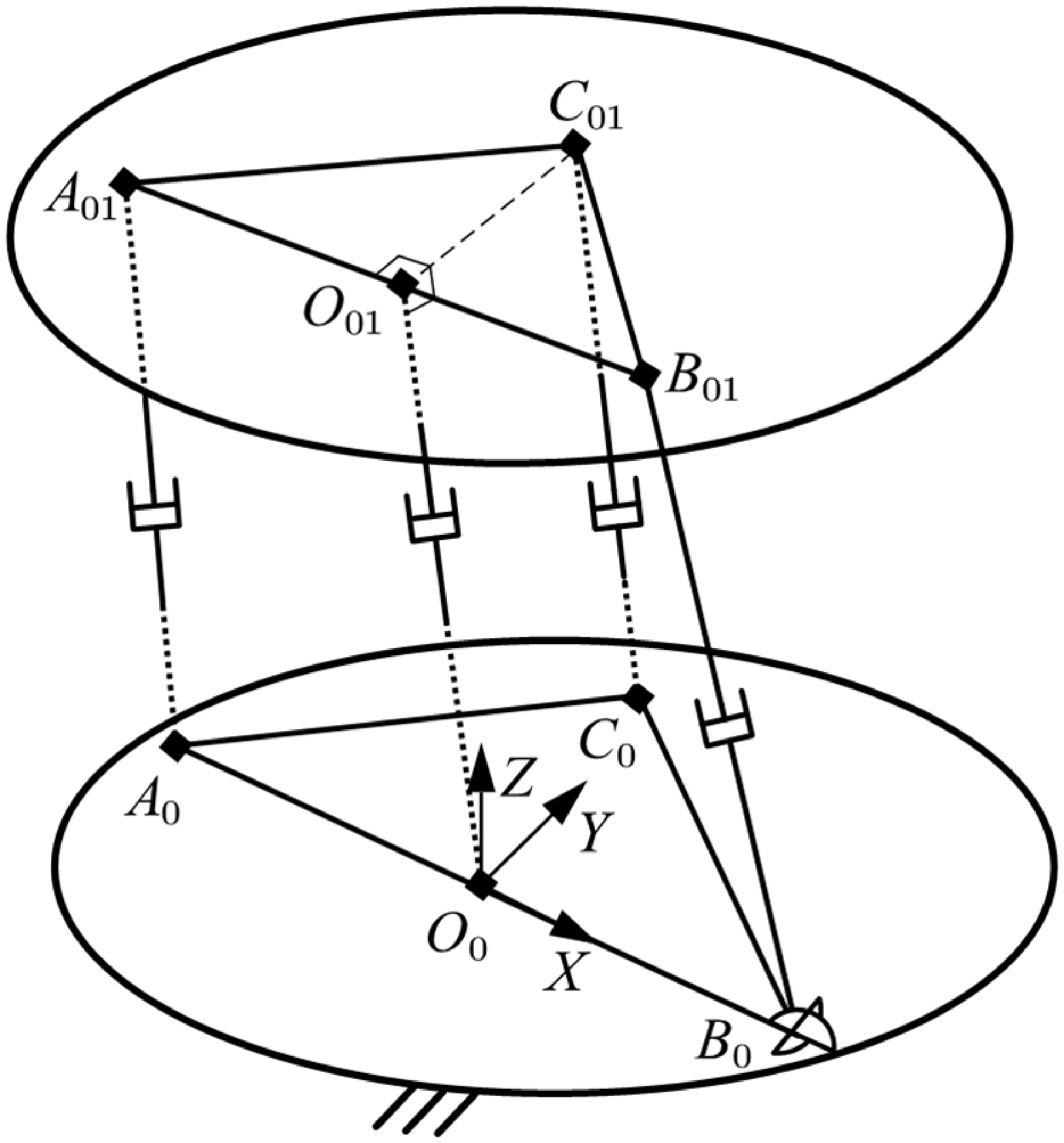
As shown in Figure 8, for this class of mechanisms, a fixed coordinate system is established with point
 $\boldsymbol{O}_{0}$
as the origin. The direction from
 $\boldsymbol{O}_{0}$
to
 $\boldsymbol{B}_{0}$
defines the
 $X$
-axis, and the direction perpendicular to the
 $X$
-axis pointing toward point
 $\boldsymbol{C}_{0}$
defines the
 $Y$
-axis.
Here, Step 1 and Step 2 are identical to those in the forward kinematic analysis of WoPC four-limb 2R1T mechanisms. Therefore,
 \begin{equation} \begin{array}{c} \begin{array}{ll} \boldsymbol{O}_{0}=\boldsymbol{O} &\quad \boldsymbol{A}_{0}=\boldsymbol{A} \end{array}\\ \begin{array}{lll} \boldsymbol{B}_{0}=\boldsymbol{B} &\quad \boldsymbol{C}_{0}=\boldsymbol{C} &\quad \boldsymbol{B}_{01}=\boldsymbol{B}_{1} \end{array} \end{array} \end{equation}
where
 $\boldsymbol{a}$
,
 $\boldsymbol{b}$
,
 $\boldsymbol{c}$
,
 $\boldsymbol{o}$
,
 $d_{OB}$
, and
 $d_{{BB_{1}}}$
are replaced by
 $\boldsymbol{a}_{0}$
,
 $\boldsymbol{b}_{0}$
,
 $\boldsymbol{c}_{0}$
,
 $\boldsymbol{o}_{0}$
,
 $d_{{O_{0}}{B_{0}}}$
, and
 $d_{{{B_{0}}B_{01}}}$
, respectively.
Schematic diagram of WPC four-limb 2R1T parallel mechanisms.

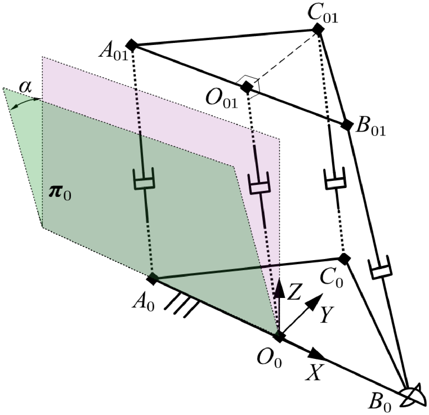
To facilitate subsequent calculations, plane
 $\boldsymbol{\pi }_{0}$
, which contains
 $\boldsymbol{A}_{0}$
,
 $\boldsymbol{B}_{0}$
, and
 $\boldsymbol{B}_{01}$
, is represented using the inner product formulation. As illustrated in Figure 9, this plane can be regarded as the
 $XZ$
-plane rotated about the
 $X$
-axis by an angle
 $\alpha$
. Combining this with the basic expression of a plane given in Table I, we obtain:
 \begin{equation} \begin{array}{ll} \boldsymbol{n}_{\pi 0}=c\alpha \boldsymbol{e}_{2}+s\alpha \boldsymbol{e}_{3} & d=0 \end{array} \end{equation}
 \begin{equation} \boldsymbol{\pi }_{0}=\boldsymbol{n}_{\pi 0}+d\boldsymbol{e}_{\infty }. \end{equation}
Schematic diagram of plane
 $\boldsymbol{\pi }_{0}$
.

Figure 9. Long description
A diagram of a plane with labeled points and axes. The diagram features two planes, one green and one purple, intersecting at an angle. The green plane is labeled as π0 and has points A0, B0, and A01. The other plane is the XZ -plane. The intersection of the two planes is marked by the line A0A01.. The diagram includes a coordinate system with axes labeled X, Y, and Z. The angle between the two planes is labeled as α. The diagram also includes perpendicular lines and right-angle symbols indicating the relationships between the points and planes.
The point pair
 ${\boldsymbol{P}_{PA}}_{01}$
corresponding to point
 $\boldsymbol{A}_{01}$
can similarly be determined by the outer product of three surfaces; refer to Figure 4.
 \begin{equation} \boldsymbol{P}_{P{A_{01}}}=\boldsymbol{S}_{{A_{0}}{A_{01}}}\wedge \boldsymbol{S}_{{B_{01}}{A_{01}}}\wedge \boldsymbol{\pi }_{0} \end{equation}
Similar to Eqs. (24), (25), and (26), the conformal geometric expressions of
 $\boldsymbol{S}_{{{A_{0}}A_{01}}}$
,
 $\boldsymbol{S}_{{{B_{01}}A_{01}}}$
, and
 ${\boldsymbol{P}}_{PA_{01}}^{\boldsymbol{*}}$
can be readily obtained. Combined with the point pair extraction formula, this yields:
 \begin{align} \begin{array}{c} \boldsymbol{A}_{01}=\dfrac{\boldsymbol{T}_{a01b2}}{A_{a01\mathrm{var}}}+\dfrac{K_{A0}\sqrt{B_{a01\mathrm{var}}}}{A_{a01\mathrm{var}}}\boldsymbol{T}_{a01b1}\\[12pt] \begin{array}{lll} \boldsymbol{T}_{a01b1}=\boldsymbol{e}_{\infty }\cdot {\boldsymbol{P}}_{PA_{01}}^{\ast } &\quad \boldsymbol{T}_{a01b2}=\boldsymbol{T}_{a01b1}\cdot {\boldsymbol{P}}_{PA_{01}}^{\ast } &\quad A_{a01\mathrm{var}}=\boldsymbol{T}_{a01b1}\cdot \boldsymbol{T}_{a01b1} \end{array}\\[8pt] \begin{array}{ll} B_{a01\mathrm{var}}={\boldsymbol{P}}_{PA_{01}}^{\ast }\cdot {\boldsymbol{P}}_{PA_{01}}^{\ast } &\quad K_{A0}=\pm 1 \end{array} \end{array} \end{align}
Similarly to Eq. (28), the conformal geometric expression of
 $\boldsymbol{O}_{01}$
can be readily obtained.
 \begin{equation} \boldsymbol{O}_{01}=\dfrac{d_{{O_{01}}{B_{01}}}\boldsymbol{A}_{01}+d_{{O_{01}}{A_{01}}}\boldsymbol{B}_{01}}{d_{{A_{01}}{B_{01}}}}-\dfrac{d_{{O_{01}}{B_{01}}}d_{{O_{01}}{A_{01}}}}{2}\boldsymbol{e}_{\infty } \end{equation}
For point
 $\boldsymbol{C}_{01}$
, two solution approaches are available. The first involves solving via the outer product of multiple surfaces, similar to the procedure in Eqs. (29)–(34), and is not elaborated further here. The second approach utilizes motion operators, based on the inherent geometric characteristics of this class of mechanisms.
In this class of mechanisms, the line connecting points
 $\boldsymbol{C}_{01}$
and
 $\boldsymbol{O}_{01}$
is perpendicular to plane
 $\boldsymbol{\pi }_{0}$
. Consequently,
 $\boldsymbol{C}_{01}$
can be obtained from
 $\boldsymbol{O}_{01}$
via a motion operator.
 \begin{equation} \boldsymbol{C}_{01}={}^{O01}{\boldsymbol{M}}{_{C01}^{}}\boldsymbol{O}_{01}{}^{O01}{\tilde{\boldsymbol{M}}}{_{C01}^{}} \end{equation}
 \begin{align} \begin{array}{c} ^{{O_{01}}}\boldsymbol{M}_{{C_{01}}}=\boldsymbol{T}_{{O_{01}}{C_{01}}}=1-\dfrac{K_{C0}}{2}d_{{O_{01}}{C_{01}}}\boldsymbol{n}_{\pi 0}\boldsymbol{e}_{\infty }\\[10pt] K_{C0}=\pm 1 \end{array} \end{align}
In the actual solution process of
 $\boldsymbol{C}_{01}$
, all unknown parameters were treated symbolically and substituted into the computations on the Wolfram Mathematica 14 platform, with all other conditions held constant. The results indicate that the computation time for Method 2, which is based on the construction of motion operators, is approximately 0.0304554 times that of Method 1, demonstrating a significant improvement in computational efficiency. The primary reason for this discrepancy is that Method 2 circumvents complex algebraic operations such as duality operations and point-pair extraction
To further investigate the general characteristics of WPC mechanisms, the parameters
 $d_{{O_{0}}{A_{0}}}=d_{{O_{0}}{B_{0}}}$
,
 $d_{{O_{0}}{C_{0}}}$
,
 $d_{{O_{01}}{A_{01}}}=d_{{O_{01}}{B_{01}}}$
,
 $d_{{O_{01}}{C_{01}}}$
,
 $d_{{A_{0}}{A_{01}}}$
,
 $d_{{B_{0}}{B_{01}}}$
,
 $d_{{C_{0}}{C_{01}}}$
,
 $\alpha$
, and
 $\beta$
were assigned the respective ranges [25, 45], [40, 60], [15, 35], [30, 50], [100, 200], [100, 200], [100, 200], [–π, π], and [–π, π]. A total of 100 random data sets were generated, and the run times of the two methods were compared, as illustrated in Figure 10. The statistical results show that the average run time of Method 1 is 0.165257 s, while that of Method 2 is 0.127697 s. The run time of Method 2 is consistently lower than that of Method 1, corresponding to an average efficiency improvement of 22.73%. More importantly, in the process of deriving the vertex expressions, Method 2 additionally and explicitly provides a link-length constraint, which offers a favorable basis for subsequent equation modeling and constraint analysis of this class of mechanisms.
Although this is not a comparison of the entire forward kinematics algorithms, this result quantitatively demonstrates that, within the CGA framework, relying solely on geometric intersections may lead to relatively low computational efficiency. In contrast, organically integrating motion operators with geometric intersections not only significantly enhances computational performance but also facilitates a more complete characterization of the kinematic properties of the mechanism. This, in turn, highlights one of the key advantages of the proposed solution approach.
Computational time comparison of two CGA construction methods for point
 $\boldsymbol{C}_{01}$
.

The distance between points
 $\boldsymbol{C}_{01}$
and
 $\boldsymbol{C}_{0}$
constitutes an input quantity and therefore satisfies the following link-length constraint:
 \begin{equation} -2\left(\boldsymbol{C}_{0}\cdot \boldsymbol{C}_{01}\right)-{d}_{C_{0}C_{01}}^{2}=0 \end{equation}
At this point, Step 4 has been completed. Subsequently, only one additional inner product operation based on a geometric relation is required. For certain mechanisms within this class, variable elimination may still be necessary; however, this can be accomplished simply by constructing a simple resultant, as will be illustrated in the following example, thereby yielding a univariate polynomial equation, which is then solved. Finally, substituting the solution back into the parametric expressions of the moving-platform vertices determines the pose of the mechanism. The overall solution procedure is intuitive, concise, and efficient.
4.2. Forward kinematic analysis of a representative WPC mechanism
Taking Configuration II of the 2UPU-2SPR parallel mechanism as an example, the feasibility and effectiveness of the forward kinematic solution approach proposed above are derived and verified.
As shown in Figure 11, the two R-joint axes of the two SPR limbs intersect perpendicularly. The R-joint axis at
 $\boldsymbol{O}_{01}$
is collinear with
 $\boldsymbol{O}_{01}\boldsymbol{C}_{01}$
. The remaining structural details are identical to those of Configuration I and are not reiterated here.
The structural parameters of the mechanism,
 $m_{0}$
,
 $n_{0}$
,
 $m_{01}$
, and
 $n_{01}$
, correspond to
 $d_{{{O_{0}}A_{0}}}$
,
 $d_{{{O_{0}}C_{0}}}$
,
 $d_{{{O_{01}}A_{01}}}$
, and
 $d_{{{O_{01}}C_{01}}}$
, respectively. The input quantities
 $L_{01}$
,
 $L_{02}$
, and
 $L_{03}$
represent the lengths of
 $d_{{{A_{0}}A_{01}}}$
,
 $d_{{{B_{0}}B_{01}}}$
, and
 $d_{{{C_{0}}C_{01}}}$
, respectively.
Substituting
 $m_{0}$
,
 $n_{0}$
,
 $m_{01}$
,
 $n_{01}$
,
 $L_{01}$
,
 $L_{02}$
, and
 $L_{03}$
into Eqs. (43), (47), (48), (49), and (51) yields the CGA expressions for all vertices of the fixed and moving platforms, as well as the first constraint equation.
Schematic diagram of the 2UPU-2SPR (Configuration II).

Figure 11. Long description
A diagram of a parallel mechanism labeled as 2UPU-2SPR (Configuration II). The diagram features a three-dimensional structure with multiple interconnected components. Key labeled points include A0, A01, B0, B01, C0, C01, O0, and O01. The structure consists of various joints and links. The axes X, Y, and Z are marked in the figure, showing the three-dimensional coordinate system. The diagram illustrates the spatial relationships and connections between the different components.
Based on the geometric characteristics of this mechanism, as illustrated in Figure 11, within triangle
 $C_{0}A_{01}B_{01}$
,
 $C_{0}O_{01}$
is the perpendicular bisector of
 $A_{01}B_{01}$
, and
 $d_{{{C_{0}}B_{01}}}$
equals
 $d_{{{C_{0}}A_{01}}}$
, from which we obtain:
 \begin{align} \boldsymbol{A}_{01}\cdot \boldsymbol{C}_{0}-\boldsymbol{B}_{01}\cdot \boldsymbol{C}_{0}=0 \\[-10pt] \nonumber \end{align}
Substituting Eqs. (43) and (49) into Eq. (51), and Eqs. (43) and (47) into Eq. (52), yields, after simplification:
 \begin{equation} -{n}_{0}^{2}-({c}_{01x}^{2}+{c}_{01y}^{2}+{c}_{01z}^{2})+2c_{01y}n_{0}+{d}_{C_{0}C_{01}}^{2}=0 \end{equation}
 \begin{equation} 2a_{01y}n_{0}-{n}_{0}^{2}-({a}_{01x}^{2}+{a}_{01y}^{2}+{a}_{01z}^{2})=2b_{01y}n_{0}-{n}_{0}^{2}-({b}_{01x}^{2}+{b}_{01y}^{2}+{b}_{01z}^{2}) \end{equation}
In the above expressions, {
 $a_{01x}$
,
 $a_{01y}$
,
 $a_{01z}$
,
 $b_{01x}$
,
 $b_{01y}$
,
 $b_{01z}$
,
 $c_{01x}$
,
 $c_{01y}$
,
 $c_{01z}$
} are the components of
 $\boldsymbol{A}_{01}$
,
 $\boldsymbol{B}_{01}$
, and
 $\boldsymbol{C}_{01}$
with respect to the vectors {
 $\boldsymbol{e}_{1}$
,
 $\boldsymbol{e}_{2}$
,
 $\boldsymbol{e}_{3}$
}, respectively.
Expanding and simplifying Eqs. (53) and (54) yields:
 \begin{equation} h_{0}\left[\begin{array}{l} \displaystyle\sum\limits_{i=1}^{3}D_{i}\left(c\beta \right)^{i-1}+D_{4}K_{C0}c\alpha +D_{5}\left(s\beta \right)^{2}+D_{6}K_{C0}c\alpha c\beta +D_{7}s\alpha s\beta \\ + \ D_{8}\text{ s}\mathit{\alpha }s\beta c\beta -\left(d_{9}s\alpha +d_{10}s\beta +d_{11}s\alpha c\beta \right)\times K_{A0}\sqrt{\displaystyle\sum\limits_{j=12}^{14}d_{j}\left(c\beta \right)^{j-12}} \end{array}\right]=0 \end{equation}
 \begin{equation} h_{0}\left[\begin{array}{l} \displaystyle\sum\limits_{i=3}^{5}d_{i}\left(c\beta \right)^{i-3}+d_{6}\left(s\beta \right)^{2}+d_{7}s\alpha s\beta +d_{8}\text{ s}\mathit{\alpha }s\beta c\beta \\+ \left(d_{9}s\alpha +d_{10}s\beta +d_{11}s\alpha c\beta \right)\times K_{A0}\sqrt{\displaystyle\sum\limits_{i=12}^{14}d_{i}\left(c\beta \right)^{i-12}} \end{array}\right]=0 \end{equation}
Wherein,
 \begin{equation} h_{0}=\dfrac{1}{d_{1}+d_{2}c\beta } \end{equation}
In the above expressions, the coefficients
 $d_{i}$
and
 $D_{i}$
are determined by the structural and input parameters.
Letting
 $y=t(\alpha /2)$
and
 $y_{0}=t(\beta /2)$
, it follows readily from the half-angle trigonometric formula that
 $c\alpha =(1-y^{2})/(1+y^{2})$
,
 $s\alpha =(2y)/(1+y^{2})$
,
 $s\beta =(2y_{0})/(1+{y}_{0}^{2})$
, and
 $c\beta =(1-{y}_{0}^{2})/(1+{y}_{0}^{2})$
. Substituting these relations into Eqs. (55) and (56) and simplifying yields:
 \begin{equation} \sum\limits_{i=0}^{2}F_{i}\left(y_{0}\right)y^{i}=0 \end{equation}
 \begin{equation} \sum\limits_{j=0}^{2}G_{j}\left(y_{0}\right)y^{\, j}=0 \end{equation}
Wherein,
 \begin{equation} \begin{array}{c} F_{0}=t_{1}+t_{2}{y}_{0}^{2}+t_{3}{y}_{0}^{4}+t_{4}K_{A0}(y_{0}+{y}_{0}^{3})T\left(y_{0}\right)\\[6pt] \begin{array}{ll} F_{1}=t_{5}y_{0}+t_{6}{y}_{0}^{3}+\left(t_{7}+t_{8}{y}_{0}^{2}+t_{9}{y}_{0}^{4}\right)K_{A0}T\left(y_{0}\right) & F_{2}=F_{0} \end{array}\\[6pt] G_{0}=r_{1}+r_{2}{y}_{0}^{2}+r_{3}{y}_{0}^{4}+K_{C0}\left(r_{4}+r_{5}{y}_{0}^{2}+r_{6}{y}_{0}^{4}\right)+r_{7}K_{A0}(y_{0}+{y}_{0}^{3})T\left(y_{0}\right)\\[6pt] \begin{array}{ll} G_{1}=r_{8}y_{0}+r_{9}{y}_{0}^{3}+K_{A0}(r_{10}+r_{11}{y}_{0}^{2}+r_{12}{y}_{0}^{4})T\left(y_{0}\right) & \end{array}\\[6pt] G_{2}=G_{0}+K_{C0}\left(r_{13}+r_{14}{y}_{0}^{2}+r_{15}{y}_{0}^{4}\right) \end{array} \end{equation}
In the above expression,
 $T(y_{0})$
denotes a radical term involving
 $y_{0}$
, and the coefficients
 $t_{i}$
and
 $r_{i}$
are determined by the structural and input parameters.
Applying the Sylvester resultant elimination method to Eqs. (58) and (59) requires only the construction of a 4 × 4 resultant matrix, from which we obtain:
 \begin{equation} \sum\limits_{i=0}^{16}u_{i}{y}_{0}^{i}+T\left(y_{0}\right)\sum\limits_{j=0}^{15}v_{j}{y}_{0}^{\, j}=0 \end{equation}
In the above expressions, the coefficient
 $u_{i}$
is determined by the structural and input parameters, while the coefficient
 $v_{i}$
is determined by the structural parameters,
 $K_{A0}$
, and the input parameters.
Transposing, squaring, and simplifying Eq. (61) yields:
 \begin{equation} \sum\limits_{i=0}^{32}w_{i}{y}_{0}^{i}=0 \end{equation}
In the above expression,
 $w_{i}$
denotes a coefficient determined by
 $m_{0}$
,
 $n_{0}$
,
 $m_{01}$
,
 $n_{01}$
,
 $L_{01}$
,
 $L_{02}$
, and
 $L_{03}$
.
Equation (62) is a 32nd-degree univariate polynomial in terms of
 $y_{0}$
. Solving Eq. (62) yields
 $y_{0}$
. Substituting the obtained values of
 $y_{0}$
into Eqs. (58) and (59) allows the corresponding
 $y$
values to be determined. Subsequently, {
 $\alpha$
,
 $\beta$
} are obtained via the half-angle trigonometric formula. Substituting these results into Eqs. (43), (47), (48), and (49) gives the expressions for the principal vertices of the moving platform, namely
 $\boldsymbol{B}_{01}$
,
 $\boldsymbol{A}_{01}$
,
 $\boldsymbol{O}_{01}$
, and
 $\boldsymbol{C}_{01}$
. Extracting the components of the vectors {
 $\boldsymbol{e}_{1}$
,
 $\boldsymbol{e}_{2}$
,
 $\boldsymbol{e}_{3}$
} yields the three-dimensional position coordinates of each point relative to the fixed coordinate system.
Similarly, for the R(2-RPS&RP)UPS mechanism shown in Figure 7b and the 3UPS-UP mechanism shown in Figure 7c, the geometric constraint condition in Step 5 involves the distance relationship between
 $d_{{{O_{0}}A_{01}}}$
and
 $d_{{{O_{0}}B_{01}}}$
. The established equation yields a univariate polynomial equation directly, without requiring any variable elimination procedure. Due to space limitations and in order to highlight the generality of the approach, only the forward kinematic solution procedure for mechanisms requiring variable elimination is discussed in detail here.
The forward kinematics solution frameworks for both WPC and WoPC mechanisms are based on CGA and are broadly similar. However, the framework for WoPC mechanisms, although concise and requiring no elimination, cannot effectively handle WPC mechanisms. For WPC mechanisms, we organically combine geometric element intersection with motion operators to solve for the intermediate point. This significantly simplifies the subsequent derivation process. Compared with relying solely on geometric intersection, it can improve the computational efficiency of solving a single point by an average of 22.73 percent. For WoPC mechanisms, the corresponding intermediate point solving does not have the objective condition to directly adopt this method. Classifying mechanisms as WoPC or WPC is precisely the core mechanism for ensuring generality. By first identifying the type of geometric constraint, the appropriate solution path is selected, thereby achieving a concise solution procedure. This is a unified framework based on CGA that includes two differentiated solution paths.
5. Numerical examples
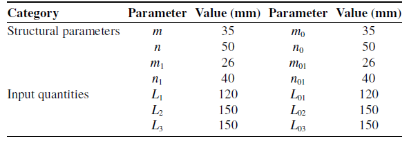
To verify the feasibility and accuracy of the forward kinematic model established for a class of four-limb 2R1T parallel mechanisms (consisting of three coplanar limbs and one spatial limb) based on CGA, a comparative analysis is conducted using actual numerical examples and three-dimensional simulation results. The structural parameters and input quantities of the mechanism are listed in Table II.
Structural parameters and input quantities of the mechanisms.

Long description
A table with two main categories: Structural parameters and Input quantities. The table has eight rows and five columns. Column headers are Category, Parameter, Value (mm), Parameter, and Value (mm). Structural parameters include m, n, m1, n1, m0, n0, m01, and n01 with values 35, 50, 26, 40, 35, 50, 26, and 40 millimeters respectively. Input quantities include L1, L2, L3, L01, L02, and L03 with values 120, 150, 150, 120, 150, and 150 millimeters respectively. Each parameter has a corresponding value in millimeters..
5.1. Numerical example for the 2UPU-2SPR (Configuration I)
Substituting the structural parameters and input quantities listed in Table II into Eq. (38) and solving the equation on the Wolfram Mathematica 14 platform yields eight solutions for
 $x$
. Applying the half-angle trigonometric formula to these solutions gives the corresponding values of
 $\beta$
. Substituting
 $\beta$
into Eqs. (37) and (42) produces the values of
 $\beta$
associated with each
 $K_{A}$
, from which the corresponding
 $x_{1}$
are determined. This process ultimately yields the solution pairs {
 $\alpha$
,
 $\beta$
} corresponding to the values of
 $K_{A}$
. Retaining only the real solutions and substituting them into Eqs. (20), (27), (28), and (34) provides the pose coordinates of the principal vertices of the moving platform, namely
 $\boldsymbol{B}_{1}$
,
 $\boldsymbol{A}_{1}$
,
 $\boldsymbol{O}_{1}$
, and
 $\boldsymbol{C}_{1}$
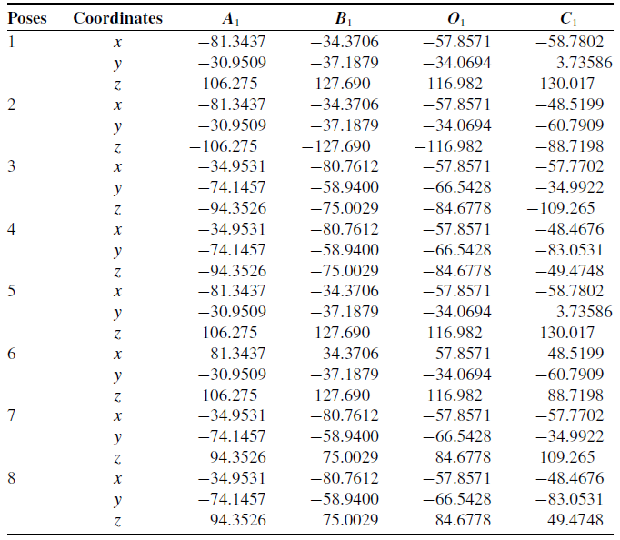
. A total of 16 real solutions are obtained, which correspond to 8 distinct real poses, as summarized in Table III.
Eight distinct real solutions for the 2UPU-2SPR (Configuration I).

Long description
A table titled ‘Eight distinct real solutions for the 2UPU-2SPR (Configuration I)’ presents the coordinates of the principal vertices of the moving platform. This table contains 24 data rows (25 rows including the header) and 6 columns. The column labels are Pose, Coordinates, A1, B1, O1, and C1. Each pose is represented by three rows, corresponding to the x, y, and z coordinates, respectively. Each row lists the coordinate value of the vertices A1, B1, O1, and C1 for that pose along the indicated axis. The table presents the 3D coordinate values of these four vertices for eight different poses.
Among these, Poses 1, 2, 3, and 4 are fully symmetric to Poses 5, 6, 7, and 8 with respect to the fixed platform, and they are consistent with the three-dimensional simulation results. Due to mechanical interference, the moving platform can only be situated below the fixed platform. Therefore, only the simulation results for the four poses in which the moving platform lies below the fixed platform are presented here, corresponding to the numerical solutions of Poses 1, 2, 3, and 4, as illustrated in Figure 12.
Mechanism poses corresponding to the four real solutions below the fixed platform for Configuration I: (a) Pose 1; (b) Pose 2; (c) Pose 3; (d) Pose 4.

5.2. Numerical example for the 2UPU-2SPR (Configuration II)
Substituting the structural parameters and input quantities listed in Table II into Eq. (62) and solving the equation on the Wolfram Mathematica 14 platform yields 32 solutions for
 $y_{0}$
. Substituting these results into Eqs. (58) and (59) yields the corresponding values of
 $y$
. Subsequently, applying the half-angle trigonometric formula produces the solution pairs {
 $\alpha$
,
 $\beta$
}, resulting in a total of 16 distinct real pairs. Retaining only the real solutions and substituting them into Eqs. (43), (47), (48), and (49) provides the pose coordinates of the principal vertices of the moving platform, namely
 $\boldsymbol{B}_{01}$
,
 $\boldsymbol{A}_{01}$
,
 $\boldsymbol{O}_{01}$
, and
 $\boldsymbol{C}_{01}$
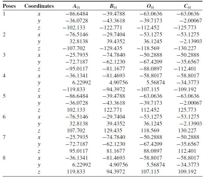
. A total of 16 real solutions are obtained, which correspond to 8 distinct real poses, as summarized in Table IV.
As with Configuration I, the moving platform of Configuration II can likewise only be situated below the fixed platform. Accordingly, only the simulation results for the four poses in which the moving platform lies below the fixed platform are presented here, corresponding to the numerical solutions of Poses 1, 2, 3, and 4, as illustrated in Figure 13.
Eight distinct real solutions for the 2UPU-2SPR (Configuration II).

Table IV. Long description
A table titled ‘Eight distinct real solutions for the 2UPU-2SPR (Configuration II)’ presents pose coordinates for eight distinct real solutions. This table contains 24 data rows (25 rows including the header) and 6 columns. The column labels are Pose, Coordinates, A01, B01, O01, and C01. Each pose is represented by three rows, corresponding to the x, y, and z coordinates, respectively. Each row lists the coordinate value of the vertices A01, B01, O01, and C01 for that pose along the indicated axis. The table presents the 3D coordinate values of these four vertices for eight different poses.
Mechanism poses corresponding to the four real solutions below the fixed platform for Configuration II: (a) Pose 1; (b) Pose 2; (c) Pose 3; (d) Pose 4.

5.3. Verification and discussion of forward kinematic solutions
In the numerical examples and model verification presented above, it can be observed from Figures 12 and 13 that, among the four real solutions corresponding to configurations in which the moving platform lies below the fixed platform for each of the two mechanisms, only one solution satisfies the non-interference condition among the components. The remaining three solutions are physically unrealizable due to mechanical interference.
Furthermore, a comparative analysis between the numerical solutions and the three-dimensional simulation results reveals that the results obtained using the CGA-based method are in excellent agreement with the three-dimensional simulation results, with the maximum absolute error of each coordinate component being substantially less than 10-8 mm. This outcome fully substantiates that the proposed solution approach, which is grounded in CGA, achieves exceptionally high computational accuracy and reliability in the forward kinematic analysis of this class of four-limb 2R1T parallel mechanisms (consisting of three coplanar limbs and one spatial limb). It thereby provides a robust kinematic foundation for subsequent dynamic analysis and control algorithm design.
Regarding the multiple-solution problem, the ability to rapidly identify the correct solution corresponding to the current configuration from the solution set is crucial for practical engineering applications. To more rapidly screen the correct solution corresponding to the physically feasible configuration, taking Configuration I in the numerical example as an example, after solving for
 $\alpha$
and
 $\beta$
, the screening can be performed using Eqs. (63) and (64). Equation (63) ensures the actual working condition that the moving platform is located below the fixed platform, thus eliminating candidate solutions that cannot be physically realized. Eq. (64) eliminates candidate solutions that could lead to mechanical interference between links and between the links and the moving platform. By substitution and calculation, the unique feasible solution consistent with the above is obtained. In practical applications, the algebraic inequalities embedded in the solution procedure can be appropriately fine-tuned to meet the current configuration of the mechanism, so as to obtain a practically realizable solution and avoid exhaustive post-screening.
 \begin{equation} \begin{array}{ll} -\pi \leq \alpha \leq \pi &\quad 0\leq \beta \leq \pi \end{array} \end{equation}
 \begin{equation} \begin{array}{ll} a_{1x}\lt b_{1x} &\quad o_{1y}\lt c_{1y} \end{array} \end{equation}
In the above expression, {
 $o_{1y}$
,
 $c_{1y}$
} are the components of
 $\boldsymbol{O}_{1}$
and
 $\boldsymbol{C}_{1}$
with respect to the vector
 $\boldsymbol{e}_{2}$
, respectively.
In ref. [Reference Zhang, Yue, Wei, Li, Liao and Xu21], the analytical forward kinematics solution for Configuration I of the 2UPU-2SPR mechanism was obtained by extracting the key geometric model and transforming the three-dimensional spatial problem into a two-dimensional planar problem. However, this method has a strong dependence on the geometric structure of the mechanism, has weak transferability to the same type of mechanism, and is not applicable to Configuration II of this mechanism. In contrast, the CGA-based forward kinematics framework proposed in this paper can simultaneously solve both configurations of the 2UPU-2SPR mechanism in a unified algebraic processing workflow and can be directly transferred to similar mechanisms, being concise and effective while more standardized and procedural. Of course, to objectively and comprehensively evaluate the engineering advantages of the CGA method proposed in this paper, it is necessary to conduct a systematic and comprehensive comparison with non-CGA methods under the same conditions and for multiple mechanism examples. This points to an important direction for future research.
Moreover, the above CGA-based forward kinematics solution framework relies on the non-degeneracy of the constructed geometric objects. When the mechanism is in a singular configuration, some geometric objects will become coincident or degenerate, and the algebraic operations may not be valid. For configurations that are close to singular but not strictly singular, the accuracy of the resulting pose solution may degrade. However, in engineering practice, parallel mechanisms are usually designed to operate far from singular configurations within their workspace. Therefore, the CGA-based solution scheme proposed in this paper can provide a stable and high-accuracy forward solution for non-singular regular configurations.
6. Conclusion
In this paper, a systematic investigation into the modeling and solution methodology for the forward kinematics of a common class of four-limb 2R1T parallel mechanisms has been conducted within the framework of CGA. Based on the geometric perpendicular relationship between the line connecting the moving-platform articulation points of the passive coplanar limb and the spatial limb, and the common plane of the three coplanar limbs, this class of mechanisms is divided into two subclasses. Differentiated CGA-based solution strategies are subsequently established for each subclass. The classification and modeling in this paper rely solely on geometric constraint characteristics, and differences in kinematic properties do not directly affect the applicability of the method. A deeper investigation into the mechanical nature of this particular geometric feature could provide valuable physical insights that complement the purely geometric treatment adopted here and would represent an interesting direction for future work.
The core characteristic of the proposed method lies in the systematic integration of motion operators with geometric intersection operations, rather than relying solely on the intersection of geometric entities. The validity of this methodological choice and its superior computational efficiency have been substantiated through numerical evaluations conducted at identical evaluation points. Although the specific solution procedures differ slightly between the two subclasses, both are fundamentally grounded in the aforementioned principle. The first subclass can be solved directly without any variable elimination, whereas the second subclass may require the supplementary use of a straightforward resultant elimination.
Numerical simulations and three-dimensional model verifications demonstrated excellent agreement, confirming that the proposed solution method is capable of yielding the complete set of real forward kinematic solutions for the mechanisms under investigation, thereby validating the accuracy and reliability of the approach.
In summary, this paper successfully adapts and applies CGA to the forward kinematics problem of four-limb 2R1T parallel mechanisms consisting of three coplanar limbs and one spatial limb. Furthermore, a unified solution framework is proposed, which is synergistically driven by motion operators and geometric intersections. The results reveal that this approach offers distinct advantages in terms of geometric meaningfulness, computational efficiency, and completeness of the solution space. This work not only provides a concise and reliable tool for the forward kinematic analysis of this class of mechanisms but also quantitatively highlights the significance of the synergistic integration of motion operators and geometric intersections within the CGA framework. Moreover, it contributes concrete algorithmic experience and empirical data for the further engineering application of CGA in the kinematic analysis of complex parallel mechanisms.
In future work, the proposed solution framework can be extended to mechanisms of the same class that are redundantly actuated or kinematically redundant and to more complex parallel mechanisms. Furthermore, the synergistic application of motion operators and geometric intersection strategies merits further investigation in the velocity and acceleration analysis of these mechanisms. Additionally, it is necessary to conduct a systematic and comprehensive comparison with non-CGA methods. The analysis of solution accuracy in the neighborhood of singular configurations will also be one of the key focuses of future research.
Supplementary material
The supplementary material for this article can be found at http://doi.org/10.1017/S0263574726104007.
Author contribution
Zhonghai Zhang supervised the research. Zhonghai Zhang and Dongyang Zhu jointly provided theoretical guidance, critically reviewed the manuscript, and proposed essential revisions. Haoming Lv performed the majority of the theoretical investigation, carried out the data processing and analysis, and drafted the initial version of the paper. All authors read and approved the final manuscript.
Financial support
This work was supported by Hebei Natural Science Foundation (Grant No. F2024202052).
Competing interest
The authors declare no conflicts of interest exist.
Ethical Approval
Not applicable.
 A1
 C1
 π0

 C01