1. Introduction
Owing to the broad scientific and technological relevance of turbulent wall flows, developing reliable ways to predict their statistical property variations with Reynolds number has received sustained attention over decades, e.g. Klewicki (Reference Klewicki2010) and Smits, McKeon & Marusic (Reference Smits, McKeon and Marusic2011). At sufficiently large Reynolds numbers, an incompressible isothermal flow along a solid surface will transition from the laminar to turbulent condition. During this transition, the flow properties evolve rapidly. Once in the turbulent regime, the statistical properties of the flow continue to exhibit variations with Reynolds number, but now more slowly. Because of the complicated set of dynamical mechanisms involved, Reynolds number dependencies occur in ways that are often difficult to anticipate from existing empirical evidence. In broad terms, the present effort informs the degree to which statistical properties and their scaling behaviours might be determinable by analytical means.
Predicting time-averaged behaviours often begins with an averaged form of the mean momentum equation, and from this starting point subsequently seeks to determine the structure of the mean flow – a primary need for engineering applications. Of course, this approach leads to the classical closure problem that inherently accompanies methods employing the Reynolds-averaged Navier–Stokes (RANS) equations. Here, indeterminacy results from the Reynolds stress divergence terms that appear in the RANS equations as a direct consequence of time or ensemble averaging the nonlinear advective acceleration terms.
Entire research communities have devoted their efforts toward developing modelling schemes to close the Reynolds stress tensor. e.g. Launder & Sandham (Reference Launder and Sandham2002). The resulting formulations most typically involve modelled terms containing empirical parameters that exhibit flow-specific dependencies. This reality hinders the generality of such schemes, as the accuracy of the resulting RANS simulation almost always diminishes for flows whose physics differ from the one used to determine the model parameters. In recognition of this limitation, recent approaches to RANS closure have adopted machine-learning frameworks that, for example, empirically discern functional forms for the terms in the Reynolds stress tensor that apply to more general classes of flows, e.g. Weatheritt & Sandberg (Reference Weatheritt and Sandberg2017). These methods hold promise relative to attaching physical meaning to the functional forms discerned. Like many research threads in turbulence, however, machine-learned physics are not educed from analytical consideration of the governing equations, but are found through accelerated optimization based on data. Relative to these general modelling approaches, the present effort is distinct and much narrower in scope, as it aims to clarify what might be learned about flow physics and the nature of RANS equation solutions from analytical treatment of the equations themselves. Consequently, the presentation herein also inherently assesses and clarifies the level of mathematical rigor adopted in the present analyses.
The challenge posed by these aims naturally leads one to consider the more tractable canonical wall flows and their simplified versions of the RANS equations. These include fully developed Couette, channel and pipe flows, and the flat plate boundary layer. Simplified forms of the mean momentum equation for these canonical flows continue to retain the essential indeterminacy that is associated with a single unclosed Reynolds stress gradient term. The literature on mean flow prediction schemes in these flows is extensive, with the predominant methods including those that assume some sort of phenomenological or mathematical closure hypothesis, borrow from the methods of matched asymptotic expansions, or exploit the symmetry properties of the equations themselves, e.g. Klewicki (Reference Klewicki2010).
Because the present focus is on equation-based prediction of flow behaviours, methods that invoke a closure hypothesis a priori are not considered in any detail. When the opportunity arises, however, connections between properties that can be discerned from analysis of the mean equations, but that are also commonly hypothesized, are made apparent and discussed.
Methods involving the use of matched asymptotic expansions have proven highly useful for constructing approximate solutions to multiscale problems, e.g. Lagerstrom (Reference Lagerstrom1988). Approaches that apply these mathematical tools to turbulent wall flows typically begin with the mean equations of motion (Mellor Reference Mellor1972; Panton Reference Panton2005). Owing to the indeterminacy of the equations, a purely analytical treatment is, however, almost immediately stymied. Such approaches can then only proceed by invoking additional assumptions. These most typically include that a two length scale inner–outer layer structure is appropriate, as well as other assumptions pertaining to the forms of the inner and outer functions, their scaling properties and the asymptotic expansions employed, e.g. Millikan (Reference Millikan1939), Mellor (Reference Mellor1972), Panton (Reference Panton2005) and Sreenivasan & Bershadskii (Reference Sreenivasan and Bershadskii2006). While not directly connected to the solutions of the RANS equations, the apparent successes of the inner–outer plus matching layer description has led to its pervasive reference within the wall-turbulence literature (Tennekes & Lumley Reference Tennekes and Lumley1972; Pope Reference Pope2000). For example, the overlap layer (described as being common to the inner and outer layers) is often used as a synonym for the logarithmic layer (inertial sublayer). Accordingly, comments regarding the findings of this approach are made at points herein.
Problems in fluid dynamics almost invariably involve questions regarding how a solution changes for variations in the relevant parameters, e.g. Reynolds number. For this reason, symmetry methods hold special importance (Hansen Reference Hansen1964; Cantwell Reference Cantwell2002). Distinct from more ad hoc approaches, those that leverage the symmetry properties of the RANS equations retain a clear mathematical basis for describing solutions to these equations. Whether symmetry considerations ultimately lead to formulations that generically address the closure challenge is, however, uncertain. In their most general application, symmetry approaches employ the machinery of Lie group theory (Cantwell Reference Cantwell2002). Relative to wall turbulence, the contributions of Oberlack and co-workers (Oberlack Reference Oberlack2001; Oberlack & Rosteck Reference Oberlack and Rosteck2010; Oberlack et al. Reference Oberlack, Waclawczyk, Rosteck and Avsarkisov2015) are perhaps most notable, as their analyses have revealed symmetry properties that are admitted by the full RANS equations. Their findings indicate that under a maximal symmetry hypothesis these equations admit a logarithmic mean profile solution, as well as other solution properties such as distance-from-the-wall scaling (Oberlack Reference Oberlack2001). In these cases and generally, however, the analysis is not able to determine the subdomain where the predicted profile properties ought to hold. The present approach suggests that this issue is tied to the local leading balance structure of the mean equation. Lie group analysis of the full RANS equations also yields its own version of the closure problem. In this case, the symmetries admitted by the RANS equations are successively augmented by a hierarchy of symmetry relations associated with a system of equations containing increasingly higher-order multipoint correlations, e.g. Oberlack et al. (Reference Oberlack, Waclawczyk, Rosteck and Avsarkisov2015).
In recent related work, She, Xi & Hussain (Reference She, Xi and Hussain2017) and Cantwell (Reference Cantwell2019) also incorporate elements of symmetry analysis. Because these studies ambitiously seek to describe the entire mean velocity profile and other statistical profiles, their analyses invoke a number of additional assumptions and ansatz. In contrast, the less ambitious but more constrained aim of the present study is to document what can be discerned with as minimal as possible input beyond the mean equations and their boundary conditions.
In connection to the present similarity analysis, it is pertinent to note that the formal application of Lie group methods is not how most of the existing laminar flow similarity solutions were found. Rather, similarity solution development has most often followed from an insightful hypothesis that was subsequently tested and possibly refined via trial and error, e.g. see Schlichting & Gersten (Reference Schlichting and Gersten2000). Generally speaking, the relevant mathematical test involves determining whether the given form of the momentum equation, along with the applicable boundary and initial conditions, are invariant under the proposed variable transformations. If they are, then the equation admits a similarity solution according to the normalizations prescribed by the variable transformations. Determining these transformations is almost always a useful outcome of the process – even if an analytical solution of the resulting invariant equation remains elusive. In the present case, this feature gains significance owing to the centrality of Reynolds number scaling to the study of wall turbulence. A broader salient point here is that the veracity and utility of the resulting invariant form (and its associated transformations) is independent of the method used to uncover it; provided, of course, that the method is analytically sound.
With the above as context, the present study employs and builds upon a multiscale analysis that has been developed for indeterminate equations. This analysis reveals that the mean equation simplified for the channel asymptotically admits an invariant form over a large wall-normal portion of the flow (Fife et al. Reference Fife, Klewicki, McMurtry and Wei2005a; Fife, Klewicki & Wei Reference Fife, Klewicki and Wei2009). Herein, we revisit, clarify and critique the analysis leading to this invariant form. Because the analysis yields a self-similar relationship between the derivatives of the mean velocity and the Reynolds shear stress, the closure problem is addressed. As a result, the invariant form yields a similarity solution for both the mean velocity and Reynolds shear stress via direct integration of the mean equation and application of the boundary conditions. These solutions hold over well-defined subdomains. For asymptotically large Reynolds number, the present similarity solutions simplify to those found via the use of matched asymptotic expansions. The spatial hierarchy of length scales inherent to these solutions allows significantly more to be discerned.
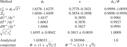
Recent high resolution direct numerical simulations (DNS) are used to investigate detailed properties of these solutions for friction Reynolds numbers up to  $8000$. The presentation extensively discusses the Fife similarity parameter,
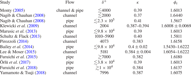
 $\phi _c$, and its behaviours at both finite and asymptotic Reynolds numbers. This parameter is directly related to the coordinate stretching inherent to generating the invariant form admitted by the mean momentum equation. A number of valid ways to estimate
 $\phi _c$ are investigated. In doing so, we also document the analytical steps and the mathematical properties of the solutions (as augmented by DNS data) relating to the conjecture by Klewicki et al. (Reference Klewicki, Philip, Marusic, Chauhan and Morrill-Winter2014) that
 $\phi _c \to \varPhi = (1 + \sqrt {5})/2$ for increasingly large Reynolds number. The connections between the channel flow invariant form and those admitted for the other canonical wall flows are briefly discussed at the close, as are the implications of the present findings to flow physics and Navier–Stokes-based modelling.
2. Analytical framework and exposition of previous results
This section clarifies what the present approach addresses, as well as what it leaves unanswered. It also documents and extends findings from a number of previous studies to set a useful context. Those familiar with the present approach should able to directly understand the findings in § 3, albeit some new analytical results are documented in § 2.2.7.
2.1. Preliminary discussion and qualifications
The analyses herein consider statistically stationary and fully developed pressure driven incompressible turbulent flow in an infinitely wide horizontal channel of height  $2 \delta$. The direction of the main flow is
 $x$. The coordinate in the wall-normal direction is
 $y$, with its origin at the lower wall. Uppercase
 $U$ denotes the time- or ensemble-averaged velocity in the
 $x$ direction, and similarly,
 $V = 0$ is the average velocity component in
 $y$. Lower case
 $u$ and
 $v$ are respectively the
 $x$ and
 $y$ velocity component fluctuations about the mean. Angle brackets denote time averaging. The starting point is the differential equation describing the mean balance of forces (per unit volume) in
 $x$, as found through Reynolds decomposition of the Navier–Stokes equation and averaging. The appropriately simplified form of this equation is given by
 \begin{equation} \rho \frac{\textrm{d}\langle uv \rangle}{\textrm{d}y} ={-}\frac{{\textrm{d}P}}{{\textrm{d}x}} + \mu\frac{\textrm{d}^2{{U}}}{{\textrm{d}y}^{2}}, \end{equation}
where  $\mu$ is the dynamic viscosity, P is the mean pressure and
 $\rho$ is the mass density. This equation indicates that the time-averaged effect of turbulent inertia (
 $TI$) on the left is balanced by the driving mean pressure gradient force (
 $PG$) and an opposing mean viscous force (
 $VF$) on the right. The boundary conditions on (2.1) are no slip at the walls and
 $\textrm {d}U/{\textrm {d}y} = \langle uv \rangle = 0$ at the channel centre. On physical grounds, the mean velocity gradient is taken to be a continuously decreasing function of
 $y$, and from this and the boundary conditions the Reynolds stress profile can be shown to integrate to zero and have a single maximum.
The present aims include clarifying the extent to which analytical methods can determine the scaling and solution properties admitted by (2.1). Toward these aims, care is taken to be clear about the non-analytically determined aspects of the present analyses and the underlying assumptions.
Channel flow turbulence is assumed to be described by a stationary ergodic process. Accordingly, the statistical structure at any given Reynolds number is taken to reflect the single observable solution to the time-averaged equations. Existing experimental and DNS results support the veracity of this assumption.
Mathematical treatment of (2.1) is hindered by at least two major challenges. One is that (2.1) is indeterminate owing to the simultaneous presence of  $U$ and
 $T = -\rho\langle uv \rangle$. As discussed in § 1, the unclosed nature of the RANS equations constitutes a persistent challenge to turbulence prediction. This challenge is addressed herein by determining a similarity relation between the wall-normal derivatives of the dependent variables in (2.1).
An arguably even bigger challenge is that the solutions to (2.1) are not unique. That is, resolving the closure problem does not ensure that the resulting solution is the one that is observed. Indeed, the prudent assumption is that a solution satisfying (2.1) is one of many possible. Non-uniqueness is not addressed analytically herein. Instead, comparisons are made between the properties of the analytically determined similarity solution and the time-averaged properties of DNS realizations. Here, the level of agreement with the observed solution and the sensitivities of the statistical properties examined characterize the quality of the evidence supporting the analytical solution. In connection with this issue it is apparent that the relationship between the instantaneous dynamics, as described by the Navier–Stokes equations, and the average statistical properties of the flow is far from clear. It is thus worth noting that the issues of indeterminacy and non-uniqueness are inherently manifest in any approach where the Navier–Stokes equation is averaged or filtered.
2.2. Mean momentum equation-based analysis
This section presents the elements of a multiscale analysis of (2.1) that lead to several key results. These provide a context for assessing the significance of the new findings that are subsequently presented. As just noted, time averaging distils the dynamics of the instantaneous motions into statistical quantities. Namely, the inertial turbulent motions that collectively generate a wall-normal transport of mean streamwise momentum are consolidated in the  $TI$ term. For an analysis of (2.1) to proceed to a solution, additional assumptions or data about the
 $TI$ term and its properties in comparison to the other terms are required. Relative to developing an analytical theory, a desirable aim is to prescribe and assume as little as possible, and to minimally rely on data.
As now described, the present approach begins with an empirical step, and thereafter uses analytical methods. Along the way, a decision is made (and justified) regarding which admissible solutions to consider. This decision effectively restricts the analysis to using the friction velocity as the single velocity scale throughout the flow. Lastly, there is a quantity,  $A$, that is directly related to
 $\phi _c$ and analytically known to be
 $O(1)$ at all Reynolds numbers. Herein, the analysis assumes (and reasons using physical and mathematical arguments) that
 $A$ attains constancy at large Reynolds number. Both the choice of characteristic velocity and the assumption that
 $A \to$ constant are shown to enjoy considerable empirical support.
2.2.1. Leading balance layers
The empirical step involves determining the leading balance structure associated with (2.1). That is, while (2.1) properly identifies the non-zero terms across the half-channel, not all of the terms are important everywhere. Thus, this situation is, for example, distinct from the mathematical representation of flow physics within the laminar boundary layer, where all of the terms in the asymptotically simplified form of the Navier–Stokes equation (i.e. Prandtl's boundary layer equation) retain leading order within the boundary layer. It does, however, bear some resemblance to the relationship between the laminar boundary layer and the outer inviscid flow where the viscous term is absent. Because there are only three terms, the leading balance structure in the channel can be made apparent by examining the ratio of the  $VF$ to
 $TI$ term across the flow. This ratio is shown in figure 1 for three friction Reynolds numbers,
 $\delta ^+ = \delta u_{\tau }/\nu$, where
 $u_{\tau } = \sqrt {\tau _w/\rho }$ is the friction velocity,
 $\tau _w = \mu (\textrm {d}U/{\textrm {d}y})|_{y = 0}$ is the mean wall shear stress and
 $\nu = \mu /\rho$ is the kinematic viscosity. Superscript ‘+’ denotes normalization by
 $\nu$ and
 $u_{\tau }$, and thus
 $y^+ = yu_{\tau }/\nu$.
Ratio of the viscous force term ( $VF$) to the turbulent inertia (
 $TI$) term in the turbulent channel flow equation (2.1);
 $\blacktriangle$,
 $\delta ^+ = 1993$;
 $\blacksquare$,
 $\delta ^+ = 3974$;
 $\bullet$,
 $\delta ^+ = 7996$. Vertical dashed lines denote the approximate boundaries of layer III at
 $\delta ^+ = 7996$, as defined by the criteria of Wei et al. (Reference Wei, Fife, Klewicki and McMurtry2005a). Data are from Yamamoto & Tsuji (Reference Yamamoto and Tsuji2018).

The simulations of Yamamoto & Tsuji (Reference Yamamoto and Tsuji2018) are used throughout the data presentations. This is because these DNS cover a large Reynolds range and maintain high spatial resolution far from the wall. The accuracy of these simulations is thus important to assessing data comparisons with the present theory. A relevant measure of the DNS accuracy is given by the residual error,  $E_R^+$, of the total stress balance (Thompson et al. Reference Thompson, Sampaio, de Bragan Alves, Thais and Mompean2016). This error includes statistical convergence and the satisfaction of statistical homogeneity in
 $x$ and
 $z$. Yamamoto & Tsuji (Reference Yamamoto and Tsuji2018) report that their
 $\delta ^+ = 7996$ simulation has an
 $E_R^+$ that is less than
 $0.005$ everywhere, and in the region where most comparisons are made herein
 $E_R^+ \le 0.0015$. Relative to the comparisons in § 3, these uncertainties are close to the differences between the DNS and the analytically based curve fits.
Figure 1 shows that the dominant balance of terms in the channel changes with wall-normal position and Reynolds number. As now described, there are four leading balance layers:  $|PG| \simeq |VF|$ (layer I),
 $|VF| \simeq |TI|$ (layer II),
 $|VF|, |TI|$ and
 $|PG|$ all leading order (layer III) and
 $|TI| \simeq |PG|$ (layer IV).
Evaluation of (2.1) at the wall reveals an exact balance between the  $VF$ and
 $PG$ terms. Owing to this, and through examination of existing low
 $\delta ^+$ data, it was at first reasoned that for all
 $\delta ^+$ there exists a layer I of
 $O(\nu /u_{\tau })$ width that essentially constitutes the traditional viscous sublayer (i.e. a layer over
 $0 \le y^+ \le 3$) e.g. Wei et al. (Reference Wei, Fife, Klewicki and McMurtry2005a) and Klewicki et al. (Reference Klewicki, Fife, Wei and McMurtry2007). Data at larger
 $\delta ^+$, such as in figure 1, however, provide evidence that the width of this layer diminishes under inner normalization with increasing
 $\delta ^+$. Thus, as
 $\delta ^+$ becomes large, the inner region of the channel apparently becomes more like planar Couette flow, where the dominant balance between the
 $TI$ and
 $VF$ terms extends to the wall at all Reynolds numbers. These higher
 $\delta ^+$ data lead one to surmise that the layer I width in channel flow is
 $\le O(\nu /u_{\tau })$. Relative to the present study, this further clarification of the layer I structure is of no consequence, as the exclusive focus herein is on mean flow behaviours significantly farther from wall.
The next layer from the wall is where the ratio  $VF/TI \simeq -1$. This is called the stress gradient balance layer (layer II) (Fife et al. Reference Fife, Klewicki, McMurtry and Wei2005a). In this layer
 $|TI| \simeq |VF|$, with the equality becoming more exact with increasing Reynolds number, e.g. Wei et al. (Reference Wei, Fife, Klewicki and McMurtry2005a). The data of figure 1 show that the inner-normalized width of layer II increases with
 $\delta ^+$. This fact does not comport with the assumption used in the traditional overlap layer based framework that this region has a width that is
 $O(\nu /u_{\tau })$ (Mellor Reference Mellor1972; Wosnik, Castillo & George Reference Wosnik, Castillo and George2000; Panton Reference Panton2005).
The outer edge of layer II is characterized by a rapid variation where  $VF/TI \to -\infty$. This ratio then reappears from
 $+\infty$, and with increasing
 $y^+$ becomes subdominant, approaching zero with increasing
 $\delta ^+$. The region (layer III) between where
 $VF/TI \simeq -1$ and
 $VF/TI \simeq 0$ is characterized by a leading balance that retains all three terms. Here, we note that some have identified the domain in the vicinity of
 $TI = 0$ as where there is a re-emergence of viscous effects, e.g. Sreenivasan & Sahay (Reference Sreenivasan and Sahay1997). In the mean, however, it is only the
 $TI$ term that becomes subdominant within this region, and this is only in a diminishingly narrow zone in the immediate vicinity of its zero crossing. Instantaneously, this region is characterized by a complicated mixture of viscous, inertial and pressure forces. On average, across layer III the dynamics transitions from a situation where viscous forces are of leading-order importance to one where they lose this leading-order significance. Regardless of interpretation, one can conclude that there is an exchange of mean balance across layer III: upon entering from layer II the leading balance is
 $|TI| \simeq |VF|$, while upon exiting into layer IV the leading balance is
 $|TI| \simeq |PG|$. Thus, beyond layer III the mean dynamical balance is inertially dominated. This feature rationally identifies the onset of the physical space inertial sublayer that is classically associated with a logarithmic mean velocity profile. More specifically, results from the framework employed herein lead to the expectation that logarithmic dependence emerges most assertively with Reynolds number within an interior domain (the inertial sublayer) beginning near the onset of layer IV (Wei et al. Reference Wei, Fife, Klewicki and McMurtry2005a; Klewicki, Fife & Wei Reference Klewicki, Fife and Wei2009). As later shown in § 3.2, this layer IV subdomain ranges over
 $2.6\sqrt {\delta ^+} \lesssim y^+ \lesssim 0.125\delta ^+$. Analysis of data at large Reynolds number support this prediction (Marusic et al. Reference Marusic, Monty, Hultmark and Smits2013; Vincenti et al. Reference Vincenti, Klewicki, Morrill-Winter, White and Wosnik2013; Morrill-Winter, Philip & Klewicki Reference Morrill-Winter, Philip and Klewicki2017), as do the results presented herein.
Considerably more can be determined empirically from the profiles in figure 1, and this has been done previously, e.g. Wei et al. (Reference Wei, Fife, Klewicki and McMurtry2005a) and Klewicki et al. (Reference Klewicki, Fife and Wei2009). This includes the Reynolds number dependencies of the layer widths and the velocity increments across them. Advancing the analytical treatment of (2.1), however, only requires a knowledge of the leading balance structure. Namely, that there exists a region near the wall where  $|VF| \simeq |TI|$, an outer region where
 $|PG| \simeq |TI|$ and an intermediate region where
 $|VF| \simeq |TI| \simeq |PG|$ and across which the exchange of balance transition just described occurs. As shown below, the scaling behaviours associated with the layer widths are, in order of magnitude, determinable from analysis of (2.1).
2.2.2. Reconciling the formal and actual orders of magnitude
We now describe how to appropriately normalize (2.1) in light of the leading balance information contained in figure 1. In this regard, the issue of the formal vs actual order of magnitude arises in association with (2.1) being unclosed. The actual order of magnitude of a term is evidenced by the structure indicated in figure 1, while the formal leading balance is that reflected by the specific normalized form of the equation. In this section  $u_{\tau }$ is taken to be the only velocity scale, but later we discuss the ramifications associated with other velocity scales. Operationally, the formal leading balance is found by neglecting the term associated with the small parameter,
 $\epsilon ^2 = 1/\delta ^+$, as
 $\delta ^+ \to \infty$. The aim of the following is to ensure that within each leading balance layer the normalization employed yields a formal order of magnitude commensurate with the actual order of magnitude. The terms in (2.2) are plotted vs
 $y^+$ in figure 2. These data are plotted at low
 $\delta ^+$ in order to see the
 $TI = PG$ dominant balance in layer IV.
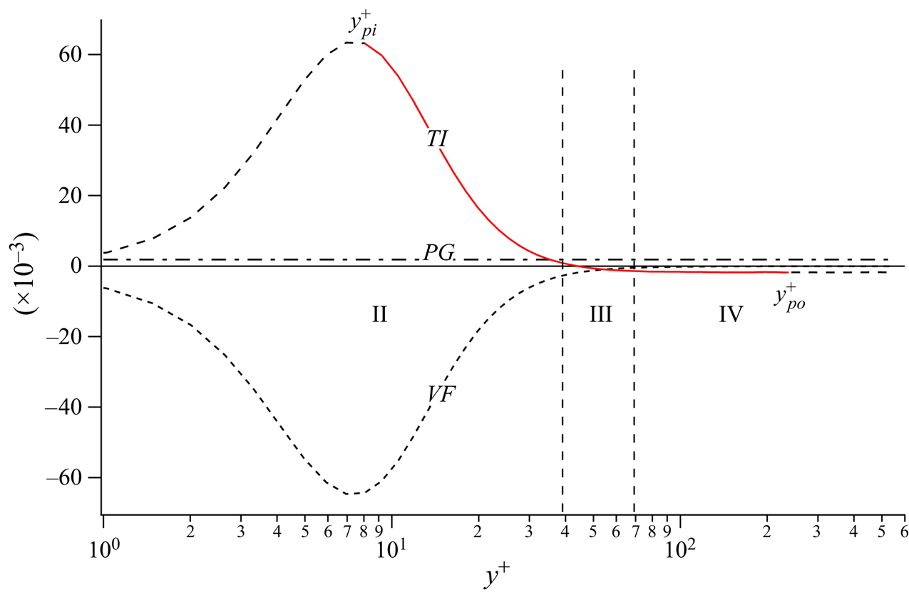
Terms in (2.2) at  $\delta ^+ = 546$. Vertical dashed lines denote the approximate boundaries of layer III. Solid (red) line portion of the
 $TI$ term profile denotes the region between its inner and outer maximum values, respectively,
 $y^+_{pi}$ and
 $y^+_{po}$, where the profile is a monotonically decreasing function. Data are from Hoyas & Jimenez (Reference Hoyas and Jimenez2006).

Since layer II extends very close to the wall as  $\delta ^+ \to \infty$, it is natural to expect that, in this region, the leading balance formally indicated by the inner-normalized form of (2.1),
 \begin{equation} 0 = \frac{\textrm{d}^2{{U^+}}}{{\textrm{d}y}^{{+}2}} + \frac{\textrm{d}T^+}{{\textrm{d}y}^+} + \epsilon^2, \end{equation}
faithfully reflects the actual leading-order balance. Given that  $\epsilon \to 0$ as
 $\delta ^+ \to \infty$, this is indeed the case. Here, the formal leading balance is
 $|TI| = |VF|$. This formal leading balance agrees with the actual layer II balance indicated in figure 1.
We now consider layer III. Over most of layer II the  $TI$ and
 $VF$ terms are much larger than
 $PG = \epsilon ^2 = 1/\delta ^+$, see figure 2. With increasing
 $y^+$, however,
 $TI$ and
 $VF$ diminish in magnitude from above and below, respectively. They eventually attain magnitudes comparable to
 $\epsilon ^2$, and the onset of layer III is marked by this condition. Across layer III, the
 $VF$ term remains negative and continues to approach zero, while the
 $TI$ term crosses zero and approaches a magnitude equal to the
 $PG$ term but of opposite sign. This condition nominally marks the end of layer III (onset of layer IV). Within layer III, all three terms have comparable magnitude, except in the region of diminishing width about the singular point were
 $TI = 0$ described above. This region centred approximately
 $TI = 0$ is not singled out for separate mathematical treatment herein.
Having established the actual magnitude ordering of terms, we now seek a rescaling of (2.2) such that all terms are formally leading order in layer III for all  $\delta ^+$, i.e. are formally
 $O(1)$. The simplest set of differential transformations that accomplish this task are used here for clarity,
 \begin{equation} {\textrm{d}y}^+ = \alpha \,\textrm{d}\tilde{y}, \quad \textrm{d}T^+ = \gamma\, \textrm{d}\tilde{T} \quad \textrm{and} \quad \textrm{d}U^+ = \textrm{d}\tilde{U}, \end{equation}
where  $\alpha$ and
 $\gamma$ are stretching parameters that must be determined. Inserting (2.3a–c) into (2.2) and demanding that all terms are
 $O(1)$ (i.e. constraining the normalized
 $PG$ term to equal 1) one obtains
 \begin{equation} 0 = \frac{\textrm{d}^2{\tilde{U}}}{\textrm{d}\tilde{y}^{2}} + \frac{\textrm{d}\tilde{T}}{\textrm{d}\tilde{y}} + 1, \end{equation}
with  $\alpha = \epsilon ^{-1}$ (
 $= \sqrt {\delta ^+}$) and
 $\gamma = \epsilon$. From this, one can readily show that the position
 $y^+ = y_m^+$ of the maximum Reynolds shear stress
 $T^+ = T_m^+$, and the inner-normalized width of layer II, are
 $O(\sqrt {\delta ^+})$. More significantly, the scalings reflected in (2.4) also hold over a finite width domain (layer III) that in viscous units is also
 $O(\sqrt {\delta ^+})$, e.g. Fife et al. (Reference Fife, Klewicki, McMurtry and Wei2005a). All of these findings have been empirically verified, i.e.
 $y_m^+$ is estimated to be approximately
 $1.6\sqrt {\delta ^+}$, while the width of layer III is estimated to be approximately
 $1.0\sqrt {\delta ^+}$, e.g. Wei et al. (Reference Wei, Fife, Klewicki and McMurtry2005a). More will be said approximately these values in § 3. In the presentation below, the rescaling step just described is replicated to derive an invariant form of (2.1) that holds to leading order over a domain of extent
 $O(\nu /u_{\tau }) < y < O(\delta )$, and within which a similarity solution is analytically shown to exist.
In layer IV the actual leading balance is between the  $TI$ and
 $PG$ terms. Commensurate with this, the traditional outer normalization (using
 $\delta$ and
 $u_{\tau }$) reflects the proper formal ordering since it positions the
 $\epsilon ^2$ term as the leading coefficient on the
 $VF$ term, i.e.
 \begin{equation} 0 = \epsilon^2\frac{\textrm{d}^2{{U^+}}}{\textrm{d}\eta^{2}} + \frac{\textrm{d}T^+}{\textrm{d}\eta} + 1, \end{equation}
where,  $\eta = y/\delta$. An important consideration pertains to how the different leading-order forms of (2.1) transition from one layer to the next. Relative to the transition from layer III to layer IV, it is a straightforward exercise to show that
 $\textrm {d}\tilde {T}/\textrm {d}\tilde {y} \equiv \textrm {d}T^+/\textrm {d}\eta$. This is relevant to some of the findings presented in § 3, since, for example, it explains why the layer III scaling (or more generally layer hierarchy scaling) for
 $T^+$ holds over a domain that starts at a
 $y^+$ position that is
 $O(\sqrt {\delta ^+})$ less than
 $y^+_m$ and extends to the channel centre at
 $y^+ = \delta ^+$ (Fife et al. Reference Fife, Wei, Klewicki and McMurtry2005b).
2.2.3. Hierarchy of scaling layers
Equation (2.1) is shown in this section to admit an invariant parameter-free form over a mathematically well-defined domain, e.g. Fife et al. (Reference Fife, Klewicki and Wei2009). The structure associated with this invariant form involves a hierarchy of scaling layers. Within well-defined bounds, each member of this layer hierarchy has a finite  $\Delta y$ extent. With increasing
 $y$ the
 $\Delta y$ width of the layers increases. Thus, in contrast to the classical two length scale construction that associates the physical space inertial sublayer with an overlap layer, the present analytical findings indicate a continuous variation in characteristic length scale. This structure naturally embraces the distance-from-the-wall scaling concept used, for example, in the simple heuristic reasoning (i.e.
 $\textrm {d}U/{\textrm {d}y} \propto u_{\tau }/y$) to arrive at a logarithmic mean profile, inherently aligns with the key assumption underlying the attached-eddy phenomenology of Townsend (Reference Townsend1976), and explains why logarithmic expansions provide accurate approximations over the hierarchy domain (Sreenivasan & Bershadskii Reference Sreenivasan and Bershadskii2006). Indeed, as demonstrated below, the present framework provides a mean equation basis for distance-from-the-wall scaling, while the results of § 3.4 provide an additional refinement to this scaling.
The layer hierarchy is formulated by recasting the  $TI$ term. This reveals the wall-normal variation in the average size of the motions contributing to turbulent momentum transport. The mathematical framework that guides this process, including the steps used to rescale (2.2) above, is codified in the method of scaling patches described by Fife et al. (Reference Fife, Klewicki, McMurtry and Wei2005a, Reference Fife, Klewicki and Wei2009). This method uses admissibility and compatibility criteria that serve to guide multiscale analysis of indeterminate equations by requiring that the normalizations over the relevant domain convey the actual leading balance structure while satisfying empirically testable boundedness criteria.
The mathematical construction begins by writing the Reynolds stress,  $T^+$, and pressure gradient,
 $\epsilon ^2$, in terms of a Reynolds stress-like quantity,
 $T^+_{\beta }$, plus a small positive parameter
 $\beta$
 \begin{equation} T^+_{\beta}(y^+) + {\beta}y^+{-} \epsilon^2y^+ = T^+(y^+). \end{equation}
From (2.6) it is apparent that the positive constant  $\beta$ is akin to
 $\epsilon ^2$ in (2.2). Indeed, when
 $\beta = \epsilon ^2$ (2.8) below identically recovers (2.2). Within a specific range of wall-normal locations, each value of
 $\beta$ uniquely corresponds to a
 $y^+$ value. To show this, we begin by differentiating (2.6) to obtain
 \begin{equation} \frac{\textrm{d}T^+_{\beta}}{{\textrm{d}y}^+} + \beta = \frac{\textrm{d}T^+}{{\textrm{d}y}^+} + \epsilon^2. \end{equation}
Subsequent insertion into (2.2) gives
 \begin{equation} 0 = \frac{\textrm{d}^2{{U^+}}}{{\textrm{d}y}^{{+}2}} + \frac{\textrm{d}T^+_{\beta}}{{\textrm{d}y}^+} + \beta. \end{equation}
Here,  $\beta$ is a constant for each
 $T^+_{\beta }$, i.e. like
 $\epsilon ^2$ is for
 $T^+$.
Analytical treatment of (2.8) focuses on the monotonically decreasing portion of the  $TI$ profile. As denoted in figure 2, the relevant region is situated between the inner and outer extrema that are respectively located at
 $y^+_{pi}$ and
 $y^+_{po}$. Limiting attention to the region of decreasing
 $TI$ ensures a one-to-one correspondence between a point on this curve and a
 $y^+$ location, i.e. it provides an unambiguous basis for stretching the wall-normal coordinate. From (2.7) it is clear that (2.8) conveys the same information as (2.2). As now illustrated, however, (2.8) allows one to expose additional properties associated (in an average sense) with the motions involved in turbulent momentum transport.
The layer III analysis of (2.2) revealed that in the vicinity of the  $TI$ zero-crossing all three terms in (2.1) are leading order, i.e.
 $O(1)$. Accordingly, a rescaling of (2.2) led to (2.4). This reconciled the formal magnitude ordering of terms in (2.2) with their actual orders of magnitude. For each
 $\beta$ within a quantifiable range of small values (corresponding to
 $y^+_{pi} < y^+ < y^+_{po}$), the
 $T^+_{\beta }$ profile of (2.6) has a single positive maximum,
 $T^+_{\beta m}$, located at a unique
 $y^+ = y^+_{\beta }$. Selecting a smaller
 $\beta$ locates
 $T^+_{\beta m}$ at larger
 $y^+ = y^+_{\beta }$, and at any given
 $T^+_{\beta m}$,
 $\textrm {d}T^+_{\beta }/{\textrm {d}y}^+ = 0$. Under this condition (2.7) becomes
 \begin{equation} \beta = \frac{\textrm{d}T^+}{{\textrm{d}y}^+} + \epsilon^2. \end{equation}
This establishes the range of  $\beta$ values corresponding to the
 $y^+$ positions between
 $y^+_{pi}$ and
 $y^+_{po}$. In the vicinity of any
 $y^+_{\beta }$ the balance of terms in (2.8) has a mathematical structure identical to that of (2.2) in the vicinity of
 $\textrm {d}T^+/{\textrm {d}y}^+ = 0$, i.e. across layer III. Thus, we surmise that every
 $y^+$ position along the decreasing portion of the
 $TI$ curve uniquely corresponds to a value of
 $\beta$, and (2.8) holds at each of these
 $y^+_{\beta }$ locations. Equation (2.8) is now rescaled at each of these locations.
Because all terms in (2.8) are of equal order in the vicinity of  $T_{\beta m}$, we seek a rescaling that formally renders each term
 $O(1)$, i.e. as was done for layer III. This is accomplished by determining the stretching coefficients,
 $\alpha (\beta )$,
 $\gamma (\beta )$ and
 $\lambda (\beta )$, associated with finite transformations
 \begin{equation} y^+ = y^+_{\beta} + \alpha \hat{y}, \quad T^+ = T^+_{\beta m} + \gamma \hat{T}(\hat{y}), \quad U^+ = U^+_{\beta} + M(y^+{-} y^+_{\beta}) + \lambda \hat{U}, \end{equation}
where superscript ‘+’ variables are functions of  $y^+$,
 $U^+_{\beta }$ is the value of
 $U^+$ at
 $y^+ = y^+_{\beta }$ and
 $M = \textrm {d}U^+_{\beta }/{\textrm {d}y}^+$. These finite transformations, and their associated differential transformations, are a generalization of those employed in rescaling (2.2) on layer III. In particular, (2.10a–c) allow for the possibility of a velocity scale other than
 $u_{\tau }$, as reflected by the stretching coefficient
 $\lambda$ in the expression involving the mean velocity.
Converting (2.10a–c) into differential transformations and inserting into (2.8) leads to
 \begin{equation} 0 = \frac{\lambda}{\alpha^2}\frac{\textrm{d}^2{\hat{U}}}{\textrm{d}\hat{y}^{2}} + \frac{\gamma}{\alpha}\frac{\textrm{d}\hat{T}}{\textrm{d}\hat{y}} + \beta, \end{equation}
where the mean derivative term containing  $M$ is not present owing to multiple differentiations. Requiring that the lead coefficients on the derivative terms in (2.11) equal
 $\beta$ yields
 \begin{equation} 0 = \frac{\textrm{d}^2{\hat{U}}}{\textrm{d}\hat{y}^{2}} + \frac{\textrm{d}\hat{T}}{\textrm{d}\hat{y}} + 1. \end{equation}
Equation (2.12) is identical in form to (2.4) and holds over a finite domain in the vicinity of each  $y^+_{\beta }$. Because transformations (2.10a–c) include the possibility of a varying velocity scale, the requirement of equal formal orders of magnitude does not uniquely determine the stretching coefficients. Namely, the coefficients
 $\alpha$ and
 $\gamma$ are now given by
 \begin{equation} \alpha = \left(\frac{\lambda}{\beta}\right)^{1/2},\quad \gamma = (\lambda \beta)^{1/2}. \end{equation}
The condition  $\lambda = 1$ corresponds to the choice of
 $u_{\tau }$ as the single velocity scale, and leads to a logarithmic mean profile solution. For
 $\lambda < 1$, a family of power law mean profile solutions are admitted, with the exponent depending on
 $\lambda$ (Fife et al. Reference Fife, Klewicki and Wei2009).
While the present framework embraces the possibility of power law solutions, from here onward we choose to only consider the  $\lambda = 1$ solutions. A primary reason for this is that the
 $\lambda = 1$ case is the only for which the inner-normalized velocity increment
 $\Delta U^+$ across layer III remains
 $O(1)$ as
 $\delta ^+ \to \infty$, and according to the primary assumption (see (2.17) below) this velocity increment asymptotically becomes constant,
 $\Delta U^+ \simeq 1.26$, see (2.34). In this regard, we note that the pipe flow measurements of McKeon (Reference McKeon2003) exhibit a
 $\Delta U^+$ increment across layer III that scatters (with no apparent
 $\delta ^+$ trend) between approximately
 $1.0$ to
 $1.4$ over the Reynolds number range
 $1800 \lesssim \delta ^+ \lesssim 530\,000$ (Klewicki Reference Klewicki2013b). A second reason is that
 $\lambda = 1$ is apparently the only case for which the solution to (2.1) becomes universal and logarithmic, while the exponent in a power law fit to data is known to vary continuously with
 $\delta ^+$, e.g. Wosnik et al. (Reference Wosnik, Castillo and George2000). The results herein pertaining to the geometric properties of the
 $T^+$ profile also provide compelling evidence that the
 $\lambda = 1$ solutions to (2.12) coincide with those that are observed. Lastly, it is perhaps relevant to note that the
 $\lambda = 1$ case corresponds to the simplest set of transformations that yields an invariant form of (2.1) on the indicated domain.
With the specification of  $\lambda = 1$, the scaling coefficients,
 $\alpha$ and
 $\gamma$, solely depend on
 $\beta$. They are also of a form identical to those used to arrive at (2.4), except
 $\epsilon ^2$ is replaced by
 $\beta$. As in the layer III analysis, the rescaling of (2.8) reveals that at each
 $y^+_{\beta }$ (i.e. at each
 $y^+$ between
 $y^+_{pi}$ and
 $y^+_{po}$) there exist a finite width domain over which that local scaling holds to leading order. In order of magnitude, the width (characteristic length) of this scaling patch is given by
 \begin{equation} W^+ = O(\beta^{{-}1/2}), \end{equation}
where at each  $y^+_{\beta }$ the value of
 $\beta$ is given by (2.9), and by virtue of (2.2)
 $\beta$ is also equal to
 $-\textrm {d}^2U^+/{\textrm {d}y}^{2+}$. Previous results demonstrate that the equality
 $W^+ = \beta ^{-1/2}$ can be used without loss of generality (Klewicki et al. Reference Klewicki, Fife and Wei2009, Reference Klewicki, Philip, Marusic, Chauhan and Morrill-Winter2014).
For large  $y^+$, the
 $W^+(y^+)$ profile becomes proportional to
 $y^+$. This feature is central to the construction of a similarity solution to (2.12), and also indicates that the present analysis framework provides a mean equation based foundation for distance-from-the-wall scaling, including why and where in the flow this scaling is expected to emerge.
2.2.4. Distance-from-the-wall scaling
Showing that  $W^+$ becomes proportional to
 $y^+$ involves determining an expression that quantifies the dependence of
 $y^+_{\beta }$ on
 $\beta$, integrating this equation and evaluating its behaviour as
 $y^+ \to \infty$. Following Fife et al. (Reference Fife, Klewicki and Wei2009), we begin with (2.7) and consider its dependence on
 $\beta$ at each
 $y^+_{\beta }$. Noting that
 $\textrm {d}T^+_{\beta }/{\textrm {d}y}^+ = 0$ at these locations, differentiation of (2.7) with respect to
 $\beta$ yields
 \begin{equation} \frac{\textrm{d}^2T^+}{{\textrm{d}y}^{{+}2}}(y^+_{\beta})\frac{{\textrm{d}y}^+_{\beta}}{\textrm{d}\beta} - 1 = 0, \end{equation}
and converting the second derivative to the scaled variables appropriate to each  $y^+_{\beta }$ gives
 \begin{equation} \beta^{3/2}\frac{\textrm{d}^2\hat{T}}{\textrm{d}\hat{y}^{2}}\Bigg|_{(\hat{y} = 0)}\frac{{\textrm{d}y}^+_{\beta}}{\textrm{d}\beta} - 1 = 0, \end{equation}
where  $\hat {y} = 0$ is located at
 $y^+_{\beta }$, see (2.10a–c).
By definition, the parameter-free functions  $\hat {T}$ and
 $\textrm {d}\hat {T}/\textrm {d}\hat {y}$ equal zero at
 $\hat {y} = 0$, and from (2.16) it is clear that the order of magnitude of
 $\textrm {d}^2\hat {T}/\textrm {d}\hat {y}^{2}$ with respect to
 $\beta$ is always
 $O(1)$. Furthermore, the transformations leading to the invariant form (2.12) satisfy the admissibility and compatibility criteria associated with the scaling patch method, as one can explicitly demonstrate that the values of the scaled functions in (2.12) are invariant at the beginning, middle and end of each
 $W^+$ layer (Fife et al. Reference Fife, Wei, Klewicki and McMurtry2005b). Morrill-Winter et al. (Reference Morrill-Winter, Philip and Klewicki2017) provide detailed empirical evidence of the invariant structure of the
 $W^+$ layers in boundary layers at large
 $\delta ^+$. Collectively, the analysis not only indicates that
 \begin{equation} -A(\beta) = \frac{\textrm{d}^2\hat{T}}{\textrm{d}\hat{y}^{2}}\Bigg|_{(\hat{y} = 0)} \end{equation}
is  $O(1)$, but naturally leads to the expectation that, over a range of
 $y^+(\beta )$ remote from
 $y^+_{pi}$ and
 $y^+_{po}$,
 $A(\beta )$ should lose any dependence on
 $\beta$ as
 $\epsilon \to 0$, i.e.
 $A(\beta )$ should approach constancy. Namely, the present construction involves an invariant equation (2.12) with invariant boundary conditions on each
 $W^+$ layer. Thus, the only apparent way to disrupt the non-constancy of
 $A$ on the hierarchy domain is through contamination at the boundaries of the hierarchy. As
 $\epsilon \to 0$, however, the number of hierarchy layers becomes large. Thus, any potential edge effects are expected to progressively diminish on an interior portion that is remote from the beginning and end points of the hierarchy domain.
Previous results (Klewicki et al. Reference Klewicki, Fife and Wei2009, Reference Klewicki, Philip, Marusic, Chauhan and Morrill-Winter2014) and those presented herein examine the veracity of  $A \to$ constant on an interior domain as
 $\epsilon \to 0$. Hereafter, the analysis treats
 $A$ as a constant, but with the recognition that the non-constancy of
 $A$ will, for example, lead to a logarithmic-like mean profile. For non-constant
 $A$, previous analyses (Fife et al. Reference Fife, Klewicki, McMurtry and Wei2005a, Reference Fife, Klewicki and Wei2009) show that
 $U^+$ is bounded from above and below by exactly logarithmic functions, with the width of the bounded region depending on the variation of
 $A$ from constancy. Overall, while there is a clear rationale for
 $A$ becoming constant as
 $\epsilon \to 0$, to date our analyses have only rigorously discerned that
 $A$ is
 $O(1)$, and thus the primary assumption of the present approach is that
 $A$ does indeed attain constancy as
 $\delta ^+ \to \infty$.
Regardless, (2.16) can be written as
 \begin{equation} \frac{{\textrm{d}y}^+_{\beta}}{\textrm{d}\beta} ={-}A^{{-}1}\beta^{{-}3/2}. \end{equation}
This expression quantifies the dependence of  $y^+_{\beta }$ on
 $\beta$. Integration of (2.18) for constant
 $A$ yields
 \begin{equation} y^+ = y^+_{\beta} ={-}A^{{-}1}\int{\beta}^{{-}3/2}\,\textrm{d}\beta = \frac{2}{A}\beta^{{-}1/2} + C_1 = \frac{2}{A}W^+\,{+}\,C_1, \end{equation}
and solving for  $W^+$
 \begin{equation} W^+ = \frac{A}{2}(y^+{-} C_1), \end{equation}
yields the result that  $W^+$ becomes proportional to
 $y^+$ at sufficiently large
 $y^+ = y^+_{\beta }$. According to the present framework, this is the origin of distance from the wall scaling; approximate at finite
 $\delta ^+$ and approaching exact proportionality as
 $y^+ \to \infty$ (
 $\delta ^+ \to \infty$).
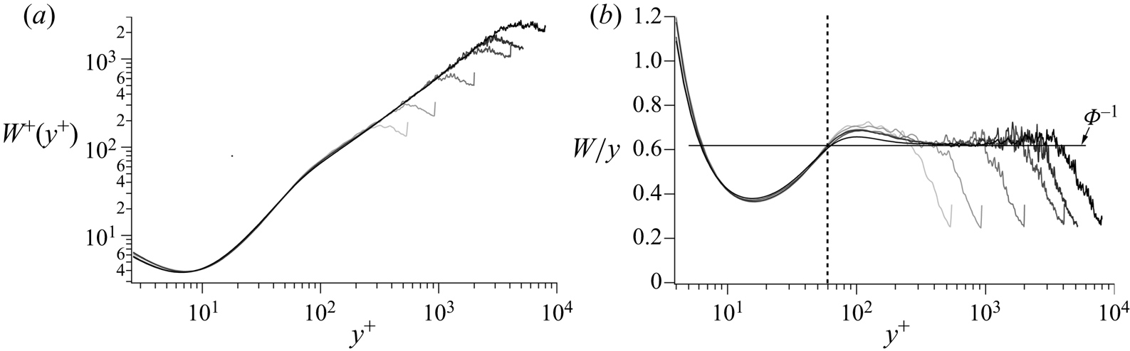
Figures 3(a) and 3(b) respectively plot  $W^+$ vs
 $y^+$ and
 $W/y$ vs
 $y^+$ over a range of existing channel flow DNS. Together these demonstrate how analytically predicted properties of the hierarchy layer width distribution emerge with increasing
 $\delta ^+$. As examined in greater detail in § 3.3, linear proportionality between
 $W^+$ and
 $y^+$ first emerges on the interior part of layer IV, and with increasing
 $\delta ^+$ the deviation from exact proportionality diminishes. The
 $W/y$ plot clearly suggests that, interior to
 $y^+ \simeq 60$, the profiles are invariant with Reynolds number, while the subsequent rise in
 $W/y$ (beyond
 $y^+ \simeq 60$) above the approximately constant value in layer IV diminishes with increasing
 $\delta ^+$. An asymptotic structure composed of only an inner region (
 $y^+ \lesssim 60$) and a
 $W/y =$ constant region has apparent consistency with the two length scale approximation employed in the inner/outer plus overlap layer construction. An approach to an inner plus
 $W/y =$ constant structure as
 $\delta ^+ \to \infty$ may in fact explain why the asymptotically reduced similarity solutions below are identical to those found using the two layer approximations. The progression toward the asymptotic flow state is, however, conceived to emerge quite differently by the two approaches. As evidenced herein, the hierarchical layer structure inherent to the similarity solutions provides additional results that can be scrutinized.
Channel flow profiles of the hierarchy layer width distribution: (a)  $W^+$ vs
 $y^+$, (b)
 $W/y$ vs
 $y^+$. Profiles increase in
 $\delta ^+$ from the lightest grey scale to darkest grey scale. Data are from the DNS of Hoyas & Jimenez (Reference Hoyas and Jimenez2006)
 $\delta ^+ = 547$,
 $934$ and
 $2004$; Pirozzoli (Reference Pirozzoli2014)
 $\delta ^+ = 4073$; Lee & Moser (Reference Lee and Moser2015)
 $\delta ^+ = 5181$; Yamamoto & Tsuji (Reference Yamamoto and Tsuji2018)
 $\delta ^+ = 7996$.

2.2.5. Fife similarity parameter
From (2.19) and (2.20) it is clear that, on the interior zone of interest,
 \begin{equation} \frac{\textrm{d}W^+}{{\textrm{d}y}^+} = \frac{A}{2} = \phi_c^{{-}1}, \quad \text{or equivalently}, \ \frac{{\textrm{d}y}^+}{\textrm{d}W^+} = \frac{2}{A} = \phi_c. \end{equation}
The second of the two forms of (2.21) is made explicit because it literally identifies the stretching of the  $y$ coordinate that underlies both the invariant form of (2.1) as given by (2.12), and through the condition for dynamical similarity (2.17) the similarity solutions to (2.12) (Klewicki & Oberlack Reference Klewicki and Oberlack2015).
Owing to the fundamental nature of this coordinate stretching, and following Klewicki (Reference Klewicki2013a) and Klewicki et al. (Reference Klewicki, Philip, Marusic, Chauhan and Morrill-Winter2014), the quantity  $\phi$ is herein called the Fife similarity parameter. This parameter generically refers to
 $\phi ^{-1} = \textrm {d}W^+/{\textrm {d}y}^+$ on the layer hierarchy domain. At any given sufficiently large Reynolds number, however, there is an interior domain where the Fife similarity parameter takes on a nearly constant value. On this domain
 $\phi$ is called
 $\phi _c$. With Reynolds number the constancy approximation of
 $\phi _c$ improves and under inner normalization the domain over which it (approximately) holds increases. Thus, the
 $\phi _c$ measured at any finite
 $\delta ^+$ changes slowly with
 $\delta ^+$ and under the primary assumption approaches a constant value as
 $\delta ^+ \to \infty$. The conjecture that this ultimate constant value is given by
 $\phi _c = \varPhi = (1 + \sqrt {5})/2$ is discussed in § 3.4. Here, we note that relative to these naming conventions it is simply a coincidence that the Greek letter for F (as in Fife) is also the same as that typically used for the golden ratio. The following analyses and results demonstrate that the Fife similarity parameter is central to describing the mathematical, physical and geometrical structure of the channel flow mean dynamics.
2.2.6. Similarity solutions
The condition for asymptotic self-similarity,  $A =$ constant (or
 $\phi = \textrm {constant}$), allows one to solve for
 $U^+$ or
 $T^+$ via direct integration and application of boundary conditions. Because the
 $A =$ constant condition closes the mean equation, arriving at one of these solutions does not involve first solving for the other. Both are independently determinable solutions to (2.1), and thus one is not subordinate to the other. (Of course, as required, both solutions adhere to all the expressions that connect
 $U^+$ and
 $T^+$.) This feature is apparently distinct from other approaches, and it provides clear justification for one to draw upon the properties of both solutions to empirically estimate
 $\phi _c$ at finite
 $\delta ^+$, or potentially determine the asymptotic value of
 $\phi _c$.
For the mean velocity we follow the approach of Klewicki & Oberlack (Reference Klewicki and Oberlack2015). In terms of inner variables,  $A$ is given by
 \begin{equation} A = \frac{2}{\phi_c} ={-}\frac{\textrm{d}^2\hat{T}}{\textrm{d}\hat{y}^{2}} ={-}\frac{\textrm{d}^2T^{+}}{{\textrm{d}y}^{{+}2}}\beta^{{-}3/2}. \end{equation}
Noting that  $\beta = - \textrm {d}^2U^+/{\textrm {d}y}^{+2}$, and using the mean vorticity transport equation for channel flow, one arrives at
 \begin{equation} \frac{2}{\phi_c} = \frac{\textrm{d}^3U^+}{{\textrm{d}y}^{{+}3}}\left(-\frac{\textrm{d}^2U^+}{{\textrm{d}y}^{{+}2}}\right)^{{-}3/2}, \end{equation}
which is an ordinary differential equation with a single dependent variable.
To solve (2.23), we treat  $\phi _c$ as a constant, and let
 $f = -\textrm {d}^2U^+/{\textrm {d}y}^{+2}$. This yields
 \begin{equation} \frac{2}{\phi_c} f^{3/2} ={-}\frac{\textrm{d}f}{{\textrm{d}y}^+}. \end{equation}
Separating variables and integrating yields,
 \begin{equation} f^{{-}1/2} = \frac{1}{\phi_c}(y^+{-} C_1). \end{equation}
The process is completed by squaring and inverting (2.25) and integrating twice to obtain
 \begin{equation} U^+(y^+) = \phi_c^2\ln(y^+{-} C_1) + C_2y^+\,{+}\, C_3, \end{equation}
where at finite  $\delta ^+$
 $C_1, C_2$ and
 $C_3$ are
 $O(1)$ and nearly constant, and, like
 $\phi _c$, as
 $\delta ^+ \to \infty$ they approach fixed values. Because
 $\textrm {d}U^+/{\textrm {d}y}^+ \to 0$ as
 $y^+ \to \infty$ it is known that
 $C_2$ also asymptotically approaches zero. Recovery of the traditional version of the logarithmic mean profile equation at finite
 $\delta ^+$, however, requires
 $C_2 \to 0$ faster than
 $1/\delta ^+$. This, and other properties of (2.26), are explored empirically in § 3. Lastly, note that
 $\phi _c^2$ appears as the leading coefficient on the logarithmic term, and thus (2.26) clarifies that
 $\phi _c^2 = 1/\kappa$, where
 $\kappa$ is the von Kármán constant.
To obtain the solution for  $T^+$ we follow the approach of Fife et al. (Reference Fife, Klewicki, McMurtry and Wei2005a, Reference Fife, Klewicki and Wei2009). First recall that
 $W^+ = \beta ^{-1/2}$,
 $\phi _c = 2/A$, and that on the hierarchy domain each
 $y^+_{\beta }$ corresponds uniquely to a
 $y^+$. Using (2.19) to solve for
 $\beta$ yields
 \begin{equation} \beta = \left( \frac{2}{A} \right)^2 (y^+{-} C_1)^{{-}2} = \frac{\phi_c^2}{(y^+\,{-}\, C_1)^2}. \end{equation}
Then, using the definition of  $\beta$ and the fact that
 $\textrm {d}T^+/{\textrm {d}y}^+ = 0$ at
 $y^+ = y_m^+$ (i.e. where
 $T^+ = T^+_m$) gives
 \begin{equation} \frac{\textrm{d}T^+}{{\textrm{d}y}^+} = \frac{\phi_c^2}{(y^+{-} C_1)^2} - \frac{1}{\delta^+} = \frac{\phi_c^2}{(y^+{-} C_1)^2} - \frac{\phi_c^2}{(y^+_m - C_1)^2}, \end{equation}
and subsequent integration yields
 \begin{equation} T^+(y^+) = C_4 - \frac{\phi_c^2}{(y^+{-} C_1)} - \frac{y^+\phi_c^2}{(y^+_m - C_1)^2}. \end{equation}
The analysis of Wei et al. (Reference Wei, McMurtry, Klewicki and Fife2005b) indicates that (2.29) is valid to leading order over a domain that begins  $O(\sqrt {\delta ^+})$ interior to
 $y_m^+$ and extends to
 $y^+ = \delta ^+$.
From the first equality of (2.28) it is straightforward to show that  $y^+_m = \lambda _m\sqrt {\delta ^+}$, and subsequent use of (2.29) allows one to show that
 $\lambda _m \to \phi _c$ like
 $1/\sqrt {\delta ^+}$ (Klewicki et al. Reference Klewicki, Philip, Marusic, Chauhan and Morrill-Winter2014). Recalling that
 $\kappa = \phi _c^{-2}$ one can see that this asymptotic result is identical to that found by Afzal (Reference Afzal1982) (i.e.
 $\lambda _m = \sqrt {1/\kappa }$) using matched asymptotic methods. It is similarly straightforward to verify that the expressions for
 $\textrm {d}U^+/{\textrm {d}y}^+$ associated with (2.26) and for
 $T^+$ in (2.29) satisfy the exact relation
 \begin{equation} \frac{\textrm{d}U^+}{{\textrm{d}y}^+} = 1 - T^+{-} \frac{y^+}{\delta^+}, \end{equation}
that derives from integrating (2.2) and applying the boundary condition at  $y^+ = 0$.
Properties of (2.26) and (2.29), and their simplified forms as  $\epsilon \to 0$, are investigated in detail in § 3.
2.2.7. Discrete hierarchy construction
The analysis above shows that each  $\beta$ value (within in its allowable range) uniquely locates both the anchor point and width of any given hierarchy layer. The
 $\Delta y^+$ widths of the layers are quantified by the
 $W^+ (y^+)$ distribution of figure 3(a). Over the layer hierarchy domain
 $y^+_{\beta }$ varies continuously, and thus there are an infinite number of layer anchor points on the interval
 $y^+_{pi} \lesssim y^+ \lesssim y^+_{po}$. Each
 $W^+(y^+)$, however, defines the finite width over which (2.12) holds to leading order. This attribute can be leveraged to significantly reduce the number of anchor points required to describe the solution properties on the hierarchy domain. Here a number of possibilities exist. An obvious constraint is that gaps between adjacent layers are not permitted. In general, a permissible construction thus requires that the anchor point of one layer resides within the bounds (end points inclusive) of at least one nearby layer, i.e. adjacent layers will generally have a finite degree of overlap. Finite overlap of adjacent layer is, however, not required. In fact, the simplest valid discrete representation of the layer hierarchy is the one in which adjacent layers abut. Attributes of this construction are now described.
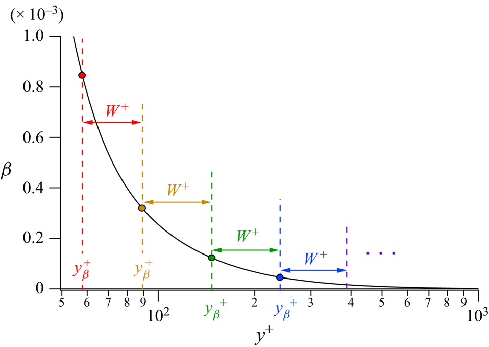
A few actual layers of the abutting layer construction are depicted in figure 4 for the  $\beta$ profile from the DNS of Yamamoto & Tsuji (Reference Yamamoto and Tsuji2018) at
 $\delta ^+ = 7996$. With increasing
 $\delta ^+$,
 $W^+$ most accurately gains proportionality with
 $y^+$ on the inertial domain. Thus, near to and within this region the
 $W^+$ layers appear approximately equal width when plotted on a logarithmic scale. The layers on the hierarchy are self-similar, and layer III is one of these layers – specifically the one for which
 $\beta = \epsilon ^2$. The asymptotic
 $y^+ = y_m^+$ position of
 $T_m^+$ is analytically known to reside at the start of layer III, and thus we accordingly choose the anchor point of each layer to be its starting point (Klewicki et al. Reference Klewicki, Philip, Marusic, Chauhan and Morrill-Winter2014). For this same reason,
 $y_m^+$ is a natural choice for one of the boundaries between abutting layers, although any
 $y^+$ on the hierarchy domain is equally valid. This fact is exploited later. As revealed through the analysis above, the coordinate transformations at any
 $y^+ = y^+_{\beta }$ retain leading-order validity over the associated
 $W^+$ extent. Under the discrete construction, the number of layers on the hierarchy increases logarithmically with Reynolds number, becoming countably infinite as
 $\delta ^+ \to \infty$.
Abutting hierarchy layers in the vicinity of  $y_m^+$ in the
 $\delta ^+ = 7996$ channel DNS of Yamamoto & Tsuji (Reference Yamamoto and Tsuji2018). Note that
 $\beta = \textrm {d}T^+/{\textrm {d}y}^+ + \epsilon ^2$. Coloured dots/dashed lines denote the anchor points for the layers having the same colour
 $W^+$.

Figure 5 illustrates the basic layer-to-layer construction. As depicted, under asymptotic conditions at any given location on the hierarchy
 \begin{equation} y^+_i + W^+_i = y^+_{i+1}. \end{equation}
By restricting attention to the  $\phi _c = 2/A$ portion of the hierarchy and neglecting the additive constant
 $C_1$ in (2.20) for asymptotically large
 $\delta ^+$, Klewicki et al. (Reference Klewicki, Philip, Marusic, Chauhan and Morrill-Winter2014) show that
 \begin{equation} y^+_i = \phi_c W^+_i, \end{equation}
and
 \begin{equation} \frac{y^+_i}{y^+_{i+1}} = \frac{W^+_i}{W^+_{i+1}} = \frac{\phi_c}{\phi_c+1}. \end{equation}
These relations reveal that on the  $\phi = \phi _c$ domain the layer widths and their anchor points comprise nested geometric series with each series having the same common ratio,
 $(\phi _c + 1)/\phi _c$.
Sketch of the  $y^+$ anchor point and associated
 $W^+$ arrangement used in the present discrete hierarchy construction.

Asymptotically, there are well-defined  $\Delta U^+|_{W^+}$ and
 $\Delta T^+|_{W^+}$ increments on any given
 $W^+$ layer. Owing to the non-overlapping property of the discrete hierarchy construction these increments respectively sum to give the overall mean velocity and Reynolds stress variations. The asymptotic reduction for the mean velocity gradient is
 $\textrm {d}U^+/{\textrm {d}y}^+ = \phi _c^2/y^+$, and use of (2.33) yields the constant velocity increment
 \begin{equation} \Delta U^+|_{W_i^+} = \int_{y_1^+}^{y_i^+\,{+}\, W_i^+} \frac{\textrm{d}U^+}{{\textrm{d}y}^+}\,{\textrm{d}y}^+ = \phi_c^2\ln\left(\frac{\phi_c + 1}{\phi_c}\right ). \end{equation}
This relation holds on the domain where  $\phi = \phi _c$ for any given
 $y^+_i$. Similarly, use of
 $y_m^+ = \phi _c\sqrt {\delta ^+}$, (2.32) and the asymptotic reduction of the Reynolds stress gradient equation (2.28) gives
 \begin{equation} \Delta T^+|_{W_i^+} = \int_{y_i^+}^{y_i^+\,{+}\, W_i^+} \frac{\textrm{d}T^+}{{\textrm{d}y}^+}\,{\textrm{d}y}^+ = \frac{\phi_c^2}{y_i^+(\phi_c + 1)} - \frac{y_i^+}{\phi_c \delta^+}. \end{equation}
Properties derived from the discrete layer hierarchy formulation, including those associated with (2.34) and (2.35) are explored and leveraged throughout § 3.
3. Results
This section first examines the behaviours of the similarity solutions (2.26) and (2.29) by comparing with DNS data up to  $\delta ^+ = 7996$. It then uses the properties of these solutions to estimate the value of the Fife similarity parameter at finite
 $\delta ^+$. Lastly, the properties of the
 $W^+$ layer hierarchy and the asymptotic version of (2.29) are used to investigate the conjecture that
 $\phi _c \to \varPhi$ as
 $\delta ^+ \to \infty$.
3.1. Assessment of similarity solutions
The solutions (2.26) and (2.29) are admitted by the invariant form of the mean momentum equation (2.12) on the layer hierarchy and under the condition that  $A(\beta )$ is a constant. In actuality,
 $A$ is not precisely constant at any finite
 $\delta ^+$, but approaches exact constancy as
 $\delta ^+ \to \infty$, apparently in accord with the rate at which the leading balances in (2.1) become exact. This situation is somewhat analogous to setting
 $\kappa$ equal to a constant in the traditional approaches used to arrive at a logarithmic mean profile equation; although
 $\phi _c$ has broader significance to the solutions of (2.1) than the slope of the
 $U^+$ profile. The solutions for
 $\hat {U}$ and
 $\hat {T}$ approach a universal form when plotted vs
 $\hat {y}$ on the
 $\phi = \phi _c$ portion of the hierarchy domain. To comport with more familiar data presentations, however, (2.26) and (2.29) and the comparisons below are made using inner variables.
3.1.1. Mean velocity solution
Figure 6(a) plots  $U^+$ vs
 $y^+$ using semi-logarithmic axes for channel flow DNS over the Reynolds number range
 $547 \le \delta ^+ \le 7996$. Figure 6(b) plots the same variables, focusing on
 $U^+$ and
 $y^+$ subranges that nominally encompass the collective inertial layers of these flows, i.e.
 $2.6\sqrt {\delta ^+} \lesssim y^+ \lesssim 0.15\delta ^+$. The DNS data are plotted in grey tones that become increasingly darker with increasing
 $\delta ^+$. Overlying these profiles are curve fits of (2.26) for
 $C_1 = 0$. Visually, the curve fits are indistinguishable from the data, and quantitatively each fit has a maximum deviation of less than
 $1$ part in
 $1000$, with the maximum deviation from the highest
 $\delta ^+$ profile equalling approximately
 $3$ parts in
 $10\,000$. Figure 6(a) generically supports the assertion that there is an emerging logarithmic layer. Relative to inner normalization, however, the closer examination in figure 6(b) makes it apparent that these curves do not follow their closest approximation to logarithmic behaviour over the same
 $y^+$ domain. In accord with the onset of layer IV, the closest adherence to a logarithmic curve begins at a
 $y^+$ location that varies like
 $\sqrt {\delta ^+}$ (Wei et al. Reference Wei, Fife, Klewicki and McMurtry2005a; Marusic et al. Reference Marusic, Monty, Hultmark and Smits2013). One consequence of this is that for two flows at disparate
 $\delta ^+$, the
 $y^+$ range of the curve fit at low
 $\delta ^+$ becomes entirely distinct from the
 $y^+$ range of the curve fit at large
 $\delta ^+$, i.e. the inertial sublayers of the two flows reside over mutually exclusive
 $y^+$ domains.
Channel flow mean velocity profiles: (a)  $U^+$ vs
 $y^+$, (b) inertial layer magnification of
 $U^+$ vs
 $y^+$. Profiles increase in
 $\delta ^+$ from the lightest grey scale to darkest grey scale. Data are from the DNS of Hoyas & Jimenez (Reference Hoyas and Jimenez2006)
 $\delta ^+ = 547$,
 $934$ and
 $2004$; Pirozzoli (Reference Pirozzoli2014)
 $\delta ^+ = 4073$; Lee & Moser (Reference Lee and Moser2015)
 $\delta ^+ = 5181$; Yamamoto & Tsuji (Reference Yamamoto and Tsuji2018)
 $\delta ^+ = 7996$. Coloured line portions indicate curve fits according to (2.26) over
 $2.6\sqrt {\delta ^+} \le y^+ \le 0.15\delta ^+$.

Relative to the present analysis of channel flow, a more objective comparison of the inertial layer profiles involves shifting both the  $U^+$ and
 $y^+$ origins to
 $y^+ = 2.6\sqrt {\delta ^+}$. As demonstrated by Klewicki & Oberlack (Reference Klewicki and Oberlack2015), when this is done the profile-to-profile variations that are apparent under inner normalization (as in figure 6a,b) are significantly reduced. The deviations from logarithmic behaviour also become most evident in the lower
 $\delta ^+$ profiles – owing primarily to the discernible effect of the linear term in (2.26). As is identifiable in figure 6(b), the three highest Reynolds number profiles exhibit a monotone straightening with
 $\delta ^+$, as the deviation from purely logarithmic dependence diminishes.
These deviations from the asymptotic (traditional) logarithmic mean profile equation,
 \begin{equation} U^+ = \phi_c^2\ln(y^+) + C_3, \end{equation}
are approximately quantified by the  $\delta ^+$ variations in the coefficients in (2.26) shown in figure 7. These variations are qualified as approximate, since the integrations that generated (2.26) are based on the precise constancy of
 $A$ (or
 $\phi _c$), and thus there is some ambiguity regarding which coefficients are mostly responsible for the deviations from the asymptotic form. As
 $\delta ^+$ becomes large, however, the coefficients approach constancy, and the influence of each becomes increasingly apparent. Recall also that these curve fits are for
 $C_1 = 0$. In this regard, Klewicki & Oberlack (Reference Klewicki and Oberlack2015) show that the effect of non-zero
 $C_1$ in (2.26) does not cause any qualitative changes, but does cause the curves for the other coefficients to shift upward or downward slightly depending on the sign of
 $C_1$. The influence of
 $C_1$ is revisited in a somewhat different context in § 3.3. In accord with the description just given, the leading coefficient in (2.26),
 $\phi _c^2$, varies considerably at low
 $\delta ^+$, but much less so for the last two
 $\delta ^+$. At
 $\delta ^+ = 7996$, the value of
 $\phi _c^2$ found from the fit of figure 6 gives
 $\phi _c^2 = 2.5661$, or equivalently,
 $\kappa = \phi _c^{-2} = 0.3897$. This is close to but slightly larger than the value of
 $0.387$ found by Yamamoto & Tsuji (Reference Yamamoto and Tsuji2018) for this data set using the traditional indicator function,
 $\varXi = y^+(\textrm {d}U^+/{\textrm {d}y}^+)$. The reasons for this deviation are described in § 3.3. The data of figure 7 indicate that
 $C_2$ decays like
 ${\sim }1/\delta ^{+2}$. This coefficient must decrease faster than
 $1/\delta ^+$ if the linear term is to become negligible at finite
 $\delta ^+$. Lastly,
 $C_3$ decreases with
 $\delta ^+$, reaching a value of
 $4.296$ at
 $\delta ^+ = 7996$. As in the boundary layer, the value for
 $C_3$ is intriguingly close to
 $\varPhi ^3$. At present, however, there are no analyses that support this observation.


Figures 8(a) and 8(b) show two different normalizations of the mean velocity gradient,  $\textrm {d}U/{\textrm {d}y}$, at
 $\delta ^+ = 7996$. Owing to the fully developed condition, this quantity is also the negative of the mean vorticity, i.e.
 $\varOmega _z = -\textrm {d}U/{\textrm {d}y}$. Figure 8(a) presents the inner-normalized profile, and uses these data to identify the best fits for
 $\phi _c$ and
 $C_1$ associated with the
 $\textrm {d}U^+/{\textrm {d}y}^+$ expression found by differentiating (2.26) and neglecting the
 $C_2$ term, see (3.5) below. Here and in figure 8(b), the exponent,
 $p$, in the curve-fit equation is set to
 $-1$. (The curve fit that allowed
 $p$ to vary yielded values of
 $p = -1.0016$ and
 $p = -0.9924$ for figures 8a and 8b, respectively.) For the reasons given in § 3.2, the curve fits across the inertial layer in this and all subsequent plots are over the domain
 $2.6\sqrt {\delta ^+} \le y^+ \le 0.125\delta ^+$. The best fit for figure 8(a) gives
 $\phi _c = 1.6117$ and
 $C_1 = -3.178$. These values are the same as found using the generalized indicator function below. The significance of the offset
 $C_1$ is discussed further relative to figure 13. The normalization of figure 8(b) directly follows from the transformations leading to (2.4). As detailed in Klewicki (Reference Klewicki2013b) and the supplementary information accompanying that study, under this normalization the mean vorticity magnitude drops from unity at the wall to
 $O(\epsilon )$ in layer III, and then across the much larger remainder of the half-channel the mean vorticity decreases to zero. The present analyses indicate that, at large Reynolds number,
 $\textrm {d}U^+/{\textrm {d}y}^+ = \phi _c^2/y^+$ at
 $y_m^+ = \phi _c \sqrt {\delta ^+}$. (Note that the classical analyses indicate this as well by setting
 $\kappa = \phi _c^{-2}$.) Accordingly, under the normalization of figure 8(b) this point is located at (
 $\phi _c$,
 $\phi _c$), and is denoted by the blue dot on figure 8(b).
Normalized mean velocity gradient profiles at  $\delta ^+ = 7996$. (a) Inner normalization: curve fit (red line) between
 $2.6\sqrt {\delta ^+} \le y^+ \le 0.125\delta ^+$ to
 $\textrm {d}U^+/{\textrm {d}y}^+ = \phi _c^2(y^+ - C_1)^{p}$ yields
 $\phi _c = 1.6117$ and
 $C_1 = -3.178$ for
 $p = -1$. (b) Normalizations based on the transformations (2.3a–c): curve fit (red line) between
 $2.6 \le y^+/\sqrt {\delta ^+} \le 11.2$ to
 $\sqrt {\delta ^+} \,\textrm {d}U^+/{\textrm {d}y}^+ = \phi _c^2(y^+/\sqrt {\delta ^+})^{p}$ yields
 $\phi _c = 1.6044$ for
 $p = -1$. Blue dot denotes the vertical and horizontal coordinates (
 $\phi _c, \phi _c$).

3.1.2. Reynolds stress solution
Figures 9(a) and 9(b) plot  $T^+ = -\langle uv \rangle ^+$ at
 $\delta ^+ = 7996$ vs
 $y^+$ on linear and logarithmic axes, respectively. In these figures the coloured segments depict the series of
 $\Delta T^+|_{W_i^+}$ increments (2.35) that begin at
 $y_m^+$. By the present theory the associated
 $\Delta y^+$ increments should equal
 $W^+$ at the given anchor points, and this is found to be the case, e.g. see figure 15 below. In accord with (2.35), the
 $\Delta T^+$ increments increase with
 $y^+$. The maximum value in this DNS profile is
 $T^+ = 0.964331$, and to within the reported number of decimals this value occurs at two adjacent
 $y^+$ positions,
 $y^+ = 144.663$ and
 $145.533$. Given that
 $y_m^+ = \phi _c\sqrt {\delta ^+}$, these two
 $y_m^+$ positions imply that
 $1.617786 \le \phi _c \le 1.627515$. These differences in the estimated
 $\phi _c$ are associated with a
 $y^+$ variation of less than
 $0.9\nu /u_{\tau }$ and thus highlight the sensitivities involved in estimating
 $\phi _c$ at finite
 $\delta ^+$ by this means. Clearly, measures other than a single peak value are desirable with regard to providing a more robust estimate of
 $\phi _c$. This issue is addressed in § 3.3.
Inner-normalized Reynolds stress profiles (grey) vs  $y^+$ at
 $\delta ^+ = 7996$: (a) linear
 $y^+$ axis, (b) logarithmic
 $y^+$ axis. Coloured segments denote the
 $\Delta T^+$ increments of successive
 $W^+$ layers beginning at
 $y_m^+$ as specified by the discrete layer hierarchy construction. Dashed line in (b) denotes curve fit of (2.29) that covers a domain beginning at the anchor point of the first discrete
 $W^+$ inside of
 $y_m^+$ and extends to
 $y/\delta = 1$. This fit uses the conjectured asymptotic parameters (
 $\phi _c = \varPhi$ and
 $C_4 = 1$), while
 $C_1$ is allowed to vary and found to be
 $0.28019$.

Consistent with the domain over which (2.29) is analytically estimated to be valid (Fife et al. Reference Fife, Wei, Klewicki and McMurtry2005b; Wei et al. Reference Wei, McMurtry, Klewicki and Fife2005b), figure 9(b) includes a plot of (2.29) from a position that begins at the anchor point of the discrete hierarchy layer ending at  $y_m^+$, and extends to
 $y/\delta = 1$. This curve fit uses the values of
 $\phi _c = \varPhi$ and
 $C_4 = 1$, while allowing
 $C_1$ to vary.
Evaluation of (2.29) for the condition  $\delta ^+ \to \infty$ leads to the prediction that
 \begin{equation} 1 - T^+_m = \frac{2\phi_c}{\sqrt{\delta^+}}, \end{equation}
or more generally,
 \begin{equation} 1 - T^+_m = C(\delta^+)^p. \end{equation}
Figure 10 presents an assessment of this analytical prediction using the DNS data of Yamamoto & Tsuji (Reference Yamamoto and Tsuji2018) over the Reynolds number range  $1000 \lesssim \delta ^+ \lesssim 8000$. An unconstrained curve fit of the data yields an exponent of
 $p = -0.520$, which differs slightly from the
 $p = -1/2$ analytical finding. Close examination indicates that the data point at
 $\delta ^+ = 3974$ seems slightly low relative to the trend of the other data on the plot. Removing this data point (not shown) supports this observation by changing the best fit exponent to
 $p = -0.513$, and under this case the four curve fits exhibit noticeably closer agreement. The other curve fits clarify the parameter sensitivities by first fixing the exponent to
 $p = -1/2$, then fixing the leading coefficient to
 $C = 2\varPhi$ which derives from
 $\phi _c = \varPhi$, and lastly holding both
 $p$ and
 $C$ fixed to the analytical values associated with
 $\phi _c = \varPhi$. Here, and in later figures, the uncertainties cited for the curve-fit parameters are
 $\pm$ one standard deviation. As is apparent, these three curve fits are visually indistinguishable. Overall, these results indicate that the primary reason for data variation from the theoretical result is tied to the value of the exponent,
 $p$.
Deviation of  $T_m^+$ from unity vs
 $\delta ^+$ for data of Yamamoto & Tsuji (Reference Yamamoto and Tsuji2018),
 $\blacksquare$. Curve fits to these data are of the form
 $1-T_m^+ = C(\delta ^+)^p$; unconstrained fit to data,
 $C = 3.777 \pm 0.228$,
 $p = -0.520 \pm 0.0213$, ——–; exponent fixed
 $p = -1/2$,
 $C = 3.249 \pm 0.0280$, ——– (green); leading coefficient fixed,
 $C = 2\varPhi = 1 + \sqrt {5} \simeq 3.236$,
 $p = -0.4999 \pm 0.0015$,
 $\cdots\cdots\cdots$ (red); conjectured asymptotic prediction,
 $C = 2\varPhi$,
 $p = -1/2$, - - - - - (blue).

The Reynolds stress gradient,  $\textrm {d}T^+/{\textrm {d}y}^+$, from the
 $\delta ^+ = 7996$ DNS is shown in figure 11. As for
 $T^+$ itself, the present similarity solution for
 $\textrm {d}T^+/{\textrm {d}y}^+$ (2.28) is predicted to hold from a position
 $y^+ = y_m^+ - O(\beta ^{-1/2})$ to the channel centre (i.e. over
 $\sqrt {\delta ^+} \lesssim y^+ \le \delta ^+$). Accordingly, the data in figure 11 are fit over this domain. The curve fits include one that is unconstrained (estimating
 $\phi _c$ and
 $C_1$), and one that is entirely prescribed using the asymptotically conjectured values of
 $\phi _c = \varPhi$ and
 $C_1 = 0$. As is apparent, both curve fits adhere closely to the data. Notably, the value of
 $C_1$ estimated via curve fit is found to be a small fraction of one viscous unit. For this reason and others, the features of this profile have advantages relative to estimating the value
 $\phi _c$ at finite
 $\delta ^+$, see § 3.3 below.
Inner-normalized Reynolds stress gradient profile vs  $y^+$ at
 $\delta ^+ = 7996$, ——– (grey), DNS; ——– (red), best fit to (2.28),
 $\phi _c = 1.6063 \pm 0.0006$,
 $C_1 = 0.1645 \pm 0.0189$; ——– (black), analytical version of (2.28) for
 $\phi _c = \varPhi = (1 + \sqrt {5})/2 = 1.618033\ldots$,
 $C_1 = 0$.

Having documented the attributes of the similarity solutions, the remainder of this section uses them to self-consistently (i) define the bounds of the inertial sublayer (i.e. at finite  $\delta ^+$ where logarithmic dependence in the
 $U^+$ profile is most emergent), (ii) empirically estimate
 $\phi _c$ at finite
 $\delta ^+$ and (iii) investigate the conjecture that the asymptotic value of
 $\phi _c$ is
 $\varPhi$.
3.2. On the bounds of the inertial sublayer
Under the construction of e.g. Millikan (Reference Millikan1939), the onset of the overlap layer (inertial sublayer) is at  $y = O(\nu /u_{\tau })$ but numerically large
 $y^+$. Similarly, the end point is at
 $y = O(\delta )$ but numerically small
 $y/\delta$. This nominal prescription pervades discussions in the literature, as well as presentations of logarithmic profile data and specifications of the domain over which
 $\kappa$ is estimated.
Based upon data such as those in figure 1, Wei et al. (Reference Wei, Fife, Klewicki and McMurtry2005a) rationally identified the onset of the inertial sublayer to be where the mean viscous force first loses leading order, i.e. where the mean dynamics first becomes inertially dominated. In doing so, they also made note of supporting data. The relevant position is located at the outer edge of layer III, or equivalently, the onset of layer IV. Wei et al. (Reference Wei, Fife, Klewicki and McMurtry2005a) empirically estimated layer IV to begin at  $y^+ \simeq 2.6\sqrt {\delta ^+}$ in channel, pipe and boundary layer flows. Regarding boundary layers, however, more recent estimates of the reconstructed mean momentum balance at larger Reynolds number indicate that layer IV begins near
 $y^+ = 3.6\sqrt {\delta ^+}$ (Morrill-Winter et al. Reference Morrill-Winter, Philip and Klewicki2017). This difference has multiple potential sources: the effect of mean inertia term vs pressure gradient in the channel, the mean flux of vorticity at the wall and its viscous annihilation in the channel, and the differing outer boundary condition between these two flows. Using mean profile data at large
 $\delta ^+$, Marusic et al. (Reference Marusic, Monty, Hultmark and Smits2013) estimate that the logarithmic layer begins near
 $y^+ = 3.1\sqrt {\delta ^+}$ for either the pipe or boundary layer, i.e. nominally half-way between the two mean momentum equation based estimates just noted.
A rational basis for specifying the end of the logarithmic layer is determinable from the present similarity solution for  $T^+$. Note that, distinct from other formulations, the present solution structure explicitly connects a logarithmic mean velocity profile to the curvature of the Reynolds stress profile, see (2.17). This allows one to use the properties of (2.28) or (2.35) to estimate the end of the logarithmic region. Practical matters associated with quantities that become too small to accurately estimate (even in DNS) also come into play. The essential observation is that (2.28) is comprised of a nonlinear term plus a constant term. Thus, with increasing
 $y^+$ the first (nonlinear) term will become increasingly smaller, until its contribution becomes negligible or beyond accurate estimation.
One way to quantify this effect is to use (2.35) to calculate the ratio of successive  $\Delta T^+$ increments. This is done for the
 $\delta ^+ = 7996$ data in figure 12. When the linear part becomes dominant
 $\Delta T^+_{i+1}/\Delta T^+_{i} \to \phi _c$. Beyond this point logarithmic behaviour will, at a minimum, become increasingly difficult to accurately quantify. The data in figure 12 indicate that this point occurs near
 $y^+ = 1000$ or
 $y/\delta \simeq 0.125$ for this flow.
Ratio of successive  $\Delta T^+$ increments at
 $\delta ^+ = 7996$ for a set of discrete hierarchy layers beginning at
 $y_m^+$. Solid curve represents a trend line.

An alternative but essentially equivalent way to estimate the end of the logarithmic layer is to use (2.28) directly. This involves monitoring the ratio of the nonlinear term to the linear term, and noting when this ratio falls below a suitably small threshold. Table 1 explores this for  $\delta ^+ = 2000, 5200$ and
 $8000$ and thresholds of
 $1/50$ and
 $1/100$. One observation is that the
 $1/50$ threshold at
 $\delta ^+ = 8000$ yields a result that is close to that indicated in figure 12. A second observation is that for a fixed threshold the
 $y/\delta$ position decreases with
 $\delta ^+$. This trend indicates that at a fixed
 $y/\delta$ the curvature of the
 $T^+$ profile becomes increasing difficult to accurately quantify with increasing
 $\delta ^+$. In this regard, the data trends in table 1 reveal that the measurable outer limit of the logarithmic layer is essentially fixed at
 $y^+ \simeq 11.5\sqrt {\delta ^+}$ or
 $y^+ \simeq 16.2\sqrt {\delta ^+}$ for thresholds of
 $1/50$ or
 $1/100$, respectively. These results indicate that the capacity of a channel DNS to accurately capture
 $\textrm {d}^2T^+/{\textrm {d}y}^{+2}$ needs to improve like
 $\sqrt {\delta ^+}$ to nominally maintain the ability to characterize the outer bound of the inertial layer at a fixed
 $y/\delta$ for increasing
 $\delta ^+$. Relative to other recent DNS it is worth noting that the
 $\delta ^+ = 7996$ of Yamamoto & Tsuji (Reference Yamamoto and Tsuji2018) moves toward this aim by maintaining high spatial resolution well beyond
 $y^+_m$.
Estimated  $y/\delta$ values at which the ratio of the linear to nonlinear terms in (2.28) falls below the indicated threshold for different
 $\delta ^+$.

Previous evidence indicates that with increasing  $\delta ^+$ the end of the layer hierarchy,
 $y^+_{po}$, remains at fixed
 $y/\delta$ (Klewicki et al. Reference Klewicki, Fife and Wei2009; Klewicki Reference Klewicki2013a,b), and thus the outer limit of the logarithmic layer is expected to scale with
 $\delta ^+$ as well. The apparent issue here is that the functions comprising
 $A(\beta )$ diminish rapidly in magnitude with increasing
 $\delta ^+$. As
 $\delta ^+$ increases, the logarithmic layer progressively moves into a region where the fixed
 $\Delta U^+$ given by (2.34) occurs over layers whose
 $W^+$ width is proportional to
 $y^+$. These increasingly spatially distributed
 $\Delta U^+$ increments are directly related to the sub-dominance of the
 $VF$ term in (2.1) on layer IV. This mathematical structure is consonant with an inertial layer that is progressively characterized by an emerging singular structure. Here, the vorticity is increasingly confined to thin boundary layer-like regions that, with increasing
 $\delta ^+$ occupy a diminishing volume fraction of the layer IV flow (Klewicki Reference Klewicki2013c). This picture is physically consistent with the observations of Meinhart & Adrian (Reference Meinhart and Adrian1995), along with the numerous subsequent studies indicating that layer IV is instantaneously populated with large scale zones of nominally uniform momentum (UMZs) that are segregated by slender regions of elevated vorticity. In this regard, it is also relevant to note that, in accord with existing measurements, the number of UMZs at any given
 $\delta ^+$ can be estimated using the present theory (Bautista et al. Reference Bautista, Ebadi, White, Chini and Klewicki2019).
The present theory predicts that the outer edge of the inertial layer scales with  $\delta ^+$. The results just presented, however, reveal that, as a practical matter, the nonlinear part of the Reynolds stress gradient underlying the existence of logarithmic dependence increasingly challenges DNS spatial resolution with increasing
 $\delta ^+$. Conversely, while all the relevant scales of motion are present in a physical experiment, only very few experimental techniques hold a realistic promise to accurately quantify higher-order derivatives at sufficient resolution, e.g. Elsnab et al. (Reference Elsnab, Monty, White, Koochesfahani and Klewicki2017). More broadly, the relevant measurement uncertainty requirements are similarly exemplified by the challenges that must be overcome to simply obtain mean velocity data that can accurately estimate
 $\kappa$ as
 $\delta ^+$ becomes large (Bailey et al. Reference Bailey, Vallikivi, Hultmark and Smits2014).
3.3. Empirically estimating  $\phi _c$ at finite $\delta ^+$


The analyses given in § 2 reveal that the Fife similarity parameter (or  $A = 2/\phi _c$) is the central parameter associated with the similarity solutions (2.26) and (2.29). Mathematically, this parameter quantifies the coordinate stretching required to cast (2.1) into its invariant form (2.12) across the scaling layer hierarchy between
 $y^+_{pi}$ and
 $y^+_{po}$. Here, it is worth restating that the associated analyses also clarify why and where distance-from-the-wall scaling becomes operative in turbulent channel flow. Through its simple connection to
 $A$, the physical significance of
 $\phi _c$ is also made apparent. Namely, dynamic self-similarity for the mean flow is precisely attained when the flux of turbulent inertial force attains exact constancy from one hierarchy layer to the next. This is the momentum based interpretation of the asymptotic
 $A(\beta ) \to$ constant condition on the inertial domain as
 $\delta ^+ \to \infty$. This mean force description is complemented by a description in terms of the mean vorticity flux (Klewicki et al. Reference Klewicki, Fife, Wei and McMurtry2007; Eyink Reference Eyink2008).
While  $\phi _c$ has the noted and apparently unique characteristics associated with the similarity solutions for
 $U^+$ and
 $T^+$, from (2.26) it is also clear that by quantifying
 $\phi _c$ one also inherently determines the value of the von Kármán constant,
 $\kappa$. The solutions, (2.26) and (2.29) offer a number of ways to estimate
 $\phi _c$. This section leverages these solutions to examine the sensitivities and other issues associated with accurately estimating
 $\phi _c$ using DNS data.
For context, it is useful to provide a listing of recent estimates of  $\kappa$ (and thus
 $\phi _c$), and this is done in table 2. Both channel and pipe flow results are included, as the present analyses predict the same asymptotic solutions for these flows. Common thought over the last half of the previous century was that
 $\kappa \simeq 0.41$ for all turbulent wall flows. Beginning approximately thirty years ago, however, a number of researchers began to question this typically cited value for
 $\kappa$, whether it was asymptotically the same for all of the canonical flows, and whether there is in fact a well-founded theoretical basis for preferring the logarithmic law over a power law, e.g. see Klewicki (Reference Klewicki2010). Owing to the advent of DNS realizations that rival or surpass typical laboratory Reynolds numbers and the development of new experimental facilities, studies over the past fifteen years have empirically addressed these questions. For example, the weight of mean profile data supports a logarithmic law, e.g. Monty (Reference Monty2005), Nagib & Chauhan (Reference Nagib and Chauhan2008) and Marusic et al. (Reference Marusic, Monty, Hultmark and Smits2013), while recent data suggest that
 $\kappa$ estimates in pipes, channels and boundary layers become increasingly similar at large
 $\delta ^+$, e.g. Marusic et al. (Reference Marusic, Monty, Hultmark and Smits2013), Vincenti et al. (Reference Vincenti, Klewicki, Morrill-Winter, White and Wosnik2013), Bailey et al. (Reference Bailey, Vallikivi, Hultmark and Smits2014), Pirozzoli (Reference Pirozzoli2014) and Lee & Moser (Reference Lee and Moser2015). The data of table 2 primarily put these estimates in the range
 $0.38 \le \kappa \le 0.39$, or equivalently,
 $1.6008 \le \phi _c \le 1.6222$.
Estimates of the Fife similarity parameter and the von Kármán constant,  $\kappa = \phi _c^{-2}$, as reported from recent channel and pipe flow studies.

A couple of entries in table 2 have specific relevance to the present analyses. Klewicki et al. (Reference Klewicki, Fife and Wei2009) were the first to estimate  $\phi _c$ using the slope of the
 $W^+$ profile. Their analysis used the DNS data of Hoyas & Jimenez (Reference Hoyas and Jimenez2006) at
 $\delta ^+ = 2004$. This method for estimating
 $\phi _c$ is the most fundamental within the context of the present theory, and it is used in figure 14 below. The result of Yamamoto & Tsuji (Reference Yamamoto and Tsuji2018) in table 2 is found from application of the traditional indicator function,
 $\varXi = y^+\textrm {d}U^+/{\textrm {d}y}^+$, to their data at
 $\delta ^+ = 7996$. In the following, methods developed from the present similarity solutions also use the data of Yamamoto & Tsuji (Reference Yamamoto and Tsuji2018) to generate alternative estimates for
 $\phi _c$.
3.3.1. Generalized indicator function
Differentiation of (2.26) yields
 \begin{equation} \frac{\textrm{d}U^+}{{\textrm{d}y}^+} = \frac{\phi_c^2}{y^+{-} C_1} + C_2, \end{equation}
which forms the basis of a comprehensive or generalized version of the indicator function,
 \begin{equation} \varXi_g = (y^+{-} C_1)\left ( \frac{\textrm{d}U^+}{{\textrm{d}y}^+} - C_2 \right ). \end{equation}
Figure 13 presents results based on (3.5) using the  $\delta ^+ = 7996$ data of Yamamoto & Tsuji (Reference Yamamoto and Tsuji2018). The curves presented include those for which (i) the optimal
 $C_1$ is found for
 $C_2 = 0$, and (ii) the optimal
 $C_2$ is found for
 $C_1 = 0$. Here, optimal is defined as the value of
 $C_1$ or
 $C_2$ that produces a linear fit to the data over
 $2.6\sqrt {\delta ^+} \le y^+ \le \delta ^+$ for which the linear term is negligible, i.e. that yields a zero slope fit. In this regard, the sensitivities of the curve-fit coefficients to (2.26) for finite Reynolds number lead to the expectation that
 $-4 \lesssim C_1 \lesssim 0.5$ and that
 $C_2$ is a very small positive number, e.g. see figure 7. Also, owing to the individual effects of
 $C_1$ and
 $C_2$ on the behaviour of
 $\varXi _g$, the two conditions plotted in figure 13 are believed to nominally bracket the possible values for
 $\phi _c$ produced from this method. As can be seen, it is similarly apparent that the best horizontal line fits of the data are convincingly and quite naturally located between the inertial layer limits identified in figure 12. The upper bound for
 $\phi _c$ from this method is approximately
 $1.6109$, while the lower bound is approximately
 $1.6016$. At any finite
 $\delta ^+$ both
 $C_1$ and
 $C_2$ will be non-zero, and thus the actual
 $\phi _c$ estimate (for the given
 $\delta ^+$) will depend on these precise values. Overall, a central result here is that small variations in
 $C_1$ or
 $C_2$ substantively influence the
 $\varXi _g$ function; effects that have no context for characterization when the traditional (asymptotic) indicator function (
 $C_1 = C_2 = 0$) is used.
Generalized indicator function (3.5) at  $\delta ^+ = 7996$: ——– (grey),
 $C_1 = C_2 = 0$; - - - - -,
 $C_1 = -3.178$,
 $C_2 = 0$; – – – –,
 $C_1 = 0$,
 $C_2 = 2.65 \times 10^{-5}$. Upper dotted line curve fit:
 $2.5950 + (2.9 \times 10^{-8})y^+$. Lower dotted line curve fit:
 $2.5651 + (7.3 \times 10^{-9})y^+$.

The findings in figure 13 indicate that the presence of undetermined constants introduces ambiguity in the accurate estimation of  $\phi _c$ using the traditionally defined
 $\varXi$. Additionally, considering an estimate that depends on a single point or small fraction of the solution profile (e.g. use of
 $y^+_m = \phi _c\sqrt {\delta ^+}$) leads one to surmise that methods that employ the overall properties of the underlying solutions are likely to produce more robust estimates. Relative to both of these considerations, estimates derived from fitting the
 $\textrm {d}T^+/{\textrm {d}y}^+$ profiles in (2.28) have some notable advantages. One is that it only relies on
 $\phi _c$ and
 $C_1$, and thus relative to
 $\varXi _g$ has one less undetermined constant. A second is that the fit of the nonlinear function (2.28) is over
 $1900$ data points. For high accuracy DNS data this latter feature produces a robust estimate. Of course, for experimental data or insufficiently accurate DNS, this method will be difficult to apply. The curve fit in figure 11 yields values for
 $C_1$ and
 $\phi _c$ of
 $0.1645$ and
 $1.6063$, respectively.
3.3.2. The $W^+(y^+)$ profile slope

The (approximately) constant slope of the function  $\phi _c^{-1} = \textrm {d}W^+/{\textrm {d}y}^+$ expresses the analytical definition of
 $\phi _c$. As is apparent, there are no other constants involved in the estimation of
 $\phi _c$ by this means. Constancy of the
 $\textrm {d}W^+/{\textrm {d}y}^+$ slope is reasoned from the present theory to emerge most rapidly on an interior-most portion of the inertial domain, i.e. over a small domain beginning near the onset of layer IV. Note that this domain begins after and ends before the domain boundaries where (2.29) is analytically predicted to hold, also see Appendix A. Figure 12 reveals that at
 $\delta ^+ = 7996$ this inertial domain resides between
 $2.6\sqrt {\delta ^+} \lesssim y^+ \lesssim 0.125\delta ^+$, and figure 14(a) shows a linear fit to the
 $W^+$ profile over this domain. While it is visually apparent that this linear fit follows the data closely, the logarithmic axes make it difficult to assess the linear fit quality in detail. For this reason, figure 14(b) presents an expanded view of the inner part of layer IV using linear axes. Figure 14(b) also presents linear fits to the
 $W^+$ profile up to
 $y/\delta = 0.15$ and
 $0.2$. For clarity, these are offset from the actual
 $W^+$ profile.
Channel flow hierarchy layer width distribution at  $\delta ^+ = 7996$: (a) full profile with linear curve fit over
 $2.6 \sqrt {\delta ^+} \lesssim y^+ \lesssim 0.125\delta ^+$,
 $\textrm {d}W^+/{\textrm {d}y}^+ = 0.6186 \pm 0.000403$ (
 $\kappa = 0.3827$); (b) close-up of linear curve fits up to
 $0.125\delta ^+$ (red), same as in (a),
 $0.15\delta ^+$ (blue)
 $\textrm {d}W^+/{\textrm {d}y}^+ = 0.6276 \pm 0.000547$ (
 $\kappa = 0.3939$),
 $0.2\delta ^+$ (green)
 $\textrm {d}W^+/{\textrm {d}y}^+ = 0.6399 \pm 0.000665$, (
 $\kappa = 0.4096$). Blue and green curve fits vertically offset for clarity.

As anticipated from the analysis, the  $W^+$ profile displays its closest adherence to linearity over the domain
 $2.6\sqrt {\delta ^+} \lesssim y^+ \lesssim 0.125\delta ^+$. Here,
 $W^+(y^+)$ also exhibits a slope having the smallest deviation from its asymptotic value, with a slope measured of
 $0.6186$ or equivalently
 $\phi _c = 1.6166$ and
 $\kappa = 0.3827$. On the other hand, the linear fits up to greater
 $y/\delta$ yield a progressively a larger slope. Thus, in addition to the greater scatter that is apparent in the profile (and anticipated from the estimation of the inertial sublayer in figure 12), the
 $W^+$ profile actually exhibits a small but detectable change in slope (i.e. has non-zero curvature) with increasing
 $y/\delta$. For reference, a second-order polynomial fit over
 $2.6\sqrt {\delta ^+} \lesssim y^+ \lesssim 0.125\delta ^+$ yields a coefficient on the quadratic term of approximately
 $2.4 \times 10^{-7}$. Given this, it is concluded that
 $\textrm {d}W^+/{\textrm {d}y}^+$ is linear over
 $2.6\sqrt {\delta ^+} \lesssim y^+ \lesssim 0.125\delta ^+$ to within less than
 $3$ parts in
 $10\,000$, with the
 $\pm 1$ standard deviation uncertainty for the slope coefficient indicating an uncertainty (scatter) of approximately
 $2$ parts in
 $1000$. Thus, this result speaks to the veracity of the primary assumption that
 $A \to$ constant (or equivalently,
 $\phi _c \to$ constant) as
 $\delta ^+ \to \infty$.
3.3.3. Geometric mean of constant $T^+$ positions

Another way to estimate  $\phi _c$ relies on the self-similar geometric structure of
 $T^+(y^+)$ in the vicinity of
 $T^+_m$. An additional analytical result is required to show this by employing the asymptotically reduced version of (2.29)
 \begin{equation} T^+(y^+) = 1 - \frac{\phi_c^2}{y^+} - \frac{y^+}{\delta^+}. \end{equation}
Note that (3.6) is also the asymptotic formula that previous researchers have determined using matched asymptotic methods (Afzal Reference Afzal1982; Panton Reference Panton2005). The present theory, however, connects this formula to the layer hierarchy as now described. Recall that (i) on the  $\phi = \phi _c$ portion of the hierarchy any
 $y^+$ location constitutes a valid anchor point for a layer of width
 $W^+ = y^+/\phi _c$, (ii) these layer widths increase according to
 $\textrm {d}W^+/{\textrm {d}y}^+ = \phi _c^{-1}$ and (iii) the
 $\hat {T}$ scaling holds from a
 $W^+$ width interior to
 $T^+_m$ to the channel centre, see figure 9. Stemming from these underlying properties, it is now shown that over the domain spanned by the layers ending and beginning at
 $y^+_m$, the geometric mean of any of the two
 $y^+$ locations at a fixed
 $T^+$ (i.e. for
 $T^+ \le T^+_m$ and
 $T^+ \ge T^+_m$) will approximate
 $y^+_m$ at finite
 $\delta ^+$, and identically come to equal
 $y^+_m$ as
 $\delta ^+ \to \infty$.
Evaluating (3.6) for  $T^+(y^+_1) = T^+(y^+_2)$
 \begin{equation} 1 - \frac{\phi_c^2}{y^+_1} - \frac{y^+_1}{\delta^+} = 1 - \frac{\phi_c^2}{y^+_2} - \frac{y^+_2}{\delta^+}, \end{equation}
which after some algebraic manipulation gives
 \begin{equation} \phi_c^2 = \frac{y^+_1 y^+_2}{\delta^+}. \end{equation}
Equation (3.8) reveals that over the given domain  $\sqrt {y^+_1 y^+_2} = \phi _c\sqrt {\delta ^+} \equiv y^+_m$, and accordingly each
 $T^+$ value yields an estimate for
 $\kappa = \delta ^+/(y^+_1 y^+_2)$. The veracity of this finding at finite
 $\delta ^+$ is investigated in figure 15, which shows a plot of the
 $T^+$ profile at
 $\delta ^+ = 7996$ in the vicinity of
 $T^+_m$. On this figure, eight horizontal lines denote fixed
 $T^+$ that nominally reside within
 $\sqrt {\delta ^+} \lesssim y^+ \lesssim \phi _c^2\sqrt {\delta ^+}$. The
 $y^+$ positions of the colour-coded discrete values of
 $T^+$ residing on the
 $T^+$ curve were determined via linear interpolation, and from these values their geometric means were computed. These geometric mean values are given by the matching coloured data points that fall very close to the vertical dashed line denoting
 $y_m^+$. More specifically, each of the eight data points displayed agree with the DNS
 $y^+_m$ value to within
 $0.5\nu /u_{\tau }$, with a total variation across the ensemble of less than
 $0.85\nu /u_{\tau }$. The average of the ensemble gives
 $\phi _c = 1.6195$ (
 $\kappa = 0.3813$).
Plot of  $T^+$ vs
 $y^+$ in the vicinity of
 $T_m^+$ at
 $\delta ^+ = 7996$ (solid grey line). Coloured data points (dots) denote the specific fixed values for
 $T^+$ on either side of
 $y^+_m$, as well as the geometric mean of these points that essentially reside on the vertical line at
 $y_m^+$. Circles (blue) denote the exact values of
 $y_1^+$ associated with selected values of
 $T^+$, and the values of
 $y_2^+$ and
 $y_m^+$ determined using the given
 $y_1^+$ and
 $\phi _{e1}$. Diamonds (red) denote the exact values of
 $y_2^+$ associated with selected values of
 $T^+$, and the values of
 $y_1^+$ and
 $y_m^+$ determined using the given
 $y_2^+$ and
 $\phi _{e2}$. Squares (black) denote the conjectured asymptotic position of
 $y^+_m$ and the discrete hierarchy layer widths that respectively precede and follow
 $y^+_m$. Maize coloured section along the
 $T^+$ profile for
 $y^+ \ge y_m^+$ denotes the
 $\Delta T^+|_{W^+}$ segment beginning at
 $y_m^+$, also see figure 9. Dashed curve along the
 $T^+$ profile is a best fit to (2.29) between
 $\sqrt {\delta ^+} \le y^+ \le \varPhi ^2\sqrt {\delta ^+}$.

3.3.4. Summary of $\phi _c$ estimates

Estimates of  $\phi _c$ from the present theory are given in table 3. The
 $\textrm {d}U^+/{\textrm {d}y}^+$ and
 $y^+_m$ estimates are from the analyses of figures 8 and 9 respectively in § 3.1. The
 $\varXi _g$ based results are respectively for the
 $C_1 = 0$ and
 $C_2 = 0$ conditions as described relative to figure 13. The
 $\textrm {d}W^+/{\textrm {d}y}^+$ based result is given for the linear fit over
 $2.6\sqrt {\delta ^+} \lesssim y^+ \lesssim 0.125\delta ^+$. Like the
 $\textrm {d}W^+/{\textrm {d}y}^+$ based estimate, the analytical finding that the geometric mean of the
 $y^+$ positions at fixed
 $T^+$ values on either side of
 $T_m^+$ (see § 3.4) does not involve any additional constants. Thus, these two methods listed in table 3 are believed to be the most accurate. Table 3 also gives the conjectured asymptotic value for
 $\phi _c$, i.e.
 $\phi _c \to \varPhi$. The last column of table 3 shows the ratio of
 $\phi _c$ to
 $\varPhi$ for the present estimates.
Estimated values of  $\phi _c$ and
 $\kappa$ at
 $\delta ^+ = 7996$ using the present theory: (i) the position of the Reynolds stress maximum, (ii) the generalized indicator function (3.5), (iii) the slope of the mean velocity gradient over
 $2.6\sqrt {\delta ^+} \lesssim y^+ \lesssim 0.125\delta ^+$, (iv) a fit to the analytically determined Reynolds stress gradient profile (2.28), (v) a linear fit to the
 $\textrm {d}W^+/{\textrm {d}y}^+$ profile over
 $2.6\sqrt {\delta ^+} \lesssim y^+ \lesssim 0.125\delta ^+$ and (vi) the average of the ensemble of geometric mean measurements,
 $y^+_m = \sqrt {y^+_1y^+_2} = \phi _c \sqrt {\delta ^+}$, associated with the constant
 $T^+$ positions in figure 15; here, the
 $\pm$ value denotes the standard deviation of the ensemble.

3.4. On the asymptotic value of $\phi _c$

The previous section provides evidence that  $\phi _c = 2/A$ approaches constancy as
 $\delta ^+$ becomes large. This agrees with the theory, and thus naturally motivates the search for an analytical determination of
 $\phi _c$ as
 $\delta ^+ \to \infty$. Klewicki et al. (Reference Klewicki, Philip, Marusic, Chauhan and Morrill-Winter2014) were the first to pursue this aim, and their efforts led to the conjecture that
 $\phi _c \to \varPhi$ as
 $\delta ^+ \to \infty$. An analytical solution still remains elusive, but properties of the similarity solutions help to clarify attributes of the conjecture. This section describes these developments.
A primary challenge facing the given objective is that while the analysis closes (2.1), it does so through the development of a self-similar relationship between functions involving derivatives of  $U^+$ and
 $T^+$. This self-similar condition leads to ratios that connect properties of one layer to the next on the
 $\phi = \phi _c$ portion of the hierarchy, e.g. (2.32) and (2.33). As a result, attempts to determine
 $\phi _c$ that employ these ratios simply recover the same ratios. This, of course, is directly related to the self-similar properties of the hierarchy, e.g. under asymptotic conditions
 $\hat {y} = y/W = \phi _c$ everywhere on the hierarchy region of interest, see figure 3(b). Boundary conditions are typically used to determine unknown constants. By definition, however, the layer hierarchy properties are realized on a domain that is remote from the flow boundaries. Thus, the desired constraint must inherently reflect the self-similar properties of the hierarchy, or otherwise comprise an independent constraint or possibly reflect asymptotic independence from constraints.
These considerations prompt the analysis below that uses the asymptotic form of (2.29), i.e. (3.6), along with the discrete hierarchy relations described in § 2.2.7 to reveal that the hierarchy structure is reflected in the geometric structure of (3.6). As described there, these also apply under asymptotic conditions. Also recall that the discrete layer construction is analytically sound since at any given anchor point on the hierarchy the invariant form (2.12) both actually and formally holds to leading order over a finite domain of width  $W^+ = O(\beta ^{-1/2})$.
We now clarify connections between the asymptotic value of  $\phi _c$ and the structure of the asymptotic
 $T^+$ solution. In the first instance this involves determining the position of the
 $W^+$ layer for which
 $\Delta T^+|_{W^+_i} = 0$. This is the case where a single (
 $n = 1$) finite width layer exactly spans the asymptotic
 $T^+(y^+)$ profile at fixed
 $T^+$. In the second instance we consider the
 $n = 2$ case, where two hierarchy layers exactly span the
 $T^+$ profile. Either case leverages the fact that (2.29) is valid from a
 $y^+$ position that is at least one
 $W^+$ layer inside of
 $y^+_m$, and on this domain
 $T^+$ passes through its peak.
3.4.1. The $\Delta T^+|_{W^+_i} = 0$ layer: a single layer spanning the $T^+$ profile


The unique discrete hierarchy layer for which  $\Delta T^+|_{W^+_i} = 0$ is now described. From (2.35), the
 $\Delta T^+|_{W^+_1} = 0$ condition is given by
 \begin{equation} 0 = \frac{\phi_c^2}{y_1^+(\phi_c + 1)} - \frac{y_1^+}{\phi_c \delta^+}. \end{equation}
Solving for  $y_1^+$ gives
 \begin{equation} y^+_1 = \phi_c\sqrt\frac{\phi_c \delta^+}{(\phi_c + 1)}, \end{equation}
which holds for  $y^+_i = y_1^+$ on the
 $\phi = \phi _c$ part of the layer hierarchy. Recalling that
 $y^+_{i} = \phi _c W^+_{i}$ gives
 \begin{equation} W^+_1 = \sqrt\frac{\phi_c \delta^+}{(\phi_c + 1)}. \end{equation}
Employing  $y^+_2 = y_1^+ + W_1^+$ and some algebraic manipulation yields
 \begin{equation} y^+_2 = (\phi_c + 1)\sqrt\frac{\phi_c \delta^+}{(\phi_c + 1)} = \sqrt{\phi_c + 1}\sqrt{\phi_c\delta^+}. \end{equation}
Invoking the previous result (3.8) confirms that
 \begin{equation} \sqrt{y^+_1y^+_2} = \phi_c\sqrt{\delta^+} = y_m^+. \end{equation}
The developments just presented indicate that (3.10), (3.12) and (3.13) hold for the  $W_i^+$ layer that has a
 $\Delta T^+|_{W_i^+} = 0$. These
 $y^+_1$ and
 $y^+_2$ values not only satisfy (3.8), but also the relation
 $y^+_1 + W^+_1 = y^+_2$, where
 $W^+_1 = y_1^+/\phi _c$. Collectively, these relations set-up the situation described in figure 15. Through (3.10), each position on the
 $T^+(y^+)$ profile for
 $y^+ < y^+_m$ is associated with a candidate or effective value of
 $\phi _c$ at the given
 $\delta ^+$. Through (3.12), each position on the
 $T^+(y^+)$ profile for
 $y^+ > y^+_m$ is similarly associated with an effective value of
 $\phi _c$. These effective values for
 $\phi _c$ associated with (3.10) and (3.12) are respectively denoted by
 $\phi _{e1}$ and
 $\phi _{e2}$ in figure 15. The symbols associated with the
 $\phi _{e1}$ are blue circles. The symbols associated with the
 $\phi _{e2}$ are red diamonds. For each
 $\phi _{e1}$, the relations (2.33) and (3.13) allow one to compute the values of
 $y_{m}^+$ and
 $y_2^+$ associated with the given
 $\phi _{e1}$. Similarly, the effective values of
 $y_{m}^+$ and
 $y_1^+$ can be determined for each
 $\phi _{e2}$. These are plotted in figure 15 for each indicated
 $\phi _{e1}$ and
 $\phi _{e2}$, also using their corresponding blue circle and red diamond symbols.
As is apparent in figure 15, the ( $y_1^+$,
 $y_m^+$,
 $y_2^+$) values associated with the
 $\phi _{e1}$ monotonically increase for increasing
 $\phi _{e1}$, and monotonically decrease for decreasing
 $\phi _{e2}$. The monotonic behaviour of the
 $\phi _{e1}$ and
 $\phi _{e2}$ curves guarantees that they cross at a single point that defines the value of
 $\phi _c$ at any given
 $\delta ^+$. Because the
 $T^+$ profile is monotonically increasing for
 $T^+ < T_m^+$ and monotonically decreasing for
 $T^+ > T_m^+$, this same uniqueness property also holds for the case in which two hierarchy layers exactly span the profile at fixed
 $T^+$, see below. Consistent with the estimates for
 $\phi _c$ in table 3, for the finite
 $\delta ^+$ profile of figure 15 these two sets of estimates agree at a
 $\phi _{e1} \simeq \phi _{e2}$ value that is very close to
 $\varPhi = (1 +\sqrt {5})/2$. This graphical display also clarifies the sensitivity of the result. For example, the results at
 $\phi _{e1} = 1.574$ and
 $1.653$ are graphically seen to be far from the correct value. Yet, they correspond to the relatively close values of
 $\kappa = 0.404$ and
 $\kappa = 0.366$, respectively.
3.4.2. Two layers spanning the $T^+$ profile

Let  $y_1^+ = b\sqrt {\delta ^+}$ specify a position (
 $y_1^+ < y_m^+$) on the
 $T^+(y^+)$ curve, where
 $b$ is a constant that is empirically known to be close to
 $1$. We now look at the conditions associated with the unique case in which two
 $W^+$ layers exactly span the
 $T^+$ profile at fixed
 $T^+$. Since there are two layers, the positions landing on the
 $T^+$ profile are denoted
 $y_1^+$ and
 $y_3^+$. Given
 $y_1^+ = b\sqrt {\delta ^+}$, repeated application of (2.31) gives
 \begin{equation} y_3^+ = \left( \frac{\phi_c + 1}{\phi_c} \right)^2 b\sqrt{\delta^+}, \end{equation}
and from (3.8)
 \begin{equation} y_1^+ y_3^+ = \left( \frac{\phi_c + 1}{\phi_c} \right)^2 b^2 \delta^+ = \phi^2 \delta^+. \end{equation}
Thus,
 \begin{equation} b = \frac{\phi_c^2}{\phi_c + 1}, \end{equation}
and, given (3.16), (3.6) yields
 \begin{equation} T^+(y_1^+) = T^+(y_3^+) = 1 - \left(\phi_c + 1 + b\right)\frac{1}{\sqrt{\delta^+}}. \end{equation}
Klewicki et al. (Reference Klewicki, Philip, Marusic, Chauhan and Morrill-Winter2014) identified the ratio  $b$ (
 $\alpha$ in that publication) relative to describing the asymptotic behaviour of
 $\phi _c$. In their analyses they evaluated some of the properties also examined herein, and empirically found that
 $b = 1.0 \pm 0.02$. The
 $n = 1$ and
 $n = 2$ analyses just presented clarify additional properties relating to how the self-similarity of the layer hierarchy structure is embedded in the
 $T^+$ profile. The present estimates of table 3 indicate that for the
 $\delta ^+ = 7996$ flow
 $b = 1$ to within a fraction of
 $1$%, as do the results in figure 15 associated with the geometric structure of the
 $T^+$ profile.
3.4.3. Implications of $b = 1$

If  $b = 1$, then
 \begin{equation} \phi_c^2 = \phi_c + 1, \end{equation}
and solving for the physically relevant positive root gives
 \begin{equation} \phi_c = \frac{1 + \sqrt{5}}{2} = \varPhi. \end{equation}
From (3.19) and (3.1) the asymptotic von Kármán constant is given by  $\kappa = 2/(3 + \sqrt {5})$.
If  $\phi _c \to \varPhi$ as
 $\delta ^+ \to \infty$ then the end points of the
 $n = 1$ case are given by
 $y_1^+ = \sqrt {\varPhi }\sqrt {\delta ^+}$ and
 $y_2^+ = \sqrt {\varPhi ^3}\sqrt {\delta ^+}$. Consistently, the
 $n = 2$ end points are given by
 $y_1^+ = \sqrt {\delta ^+}$ and
 $y_3^+ = \varPhi ^2\sqrt {\delta ^+}$, with
 $y_2^+ = y_m^+ = \varPhi \sqrt {\delta ^+}$. The asymptotic predictions for
 $W^+(\sqrt {\delta ^+})$ and
 $W^+(\varPhi \sqrt {\delta ^+})$ agree with the profile of figure 15 to within less than
 $0.2\,\%$. Consistently, relative to the
 $\Delta T^+|_{W^+_i} = 0$ layer the vertical dashed lines in figure 15 demonstrate that the values of
 $y_1^+$ and
 $y_2^+$ using
 $\varPhi$ are essentially indistinguishable from those using
 $\phi _c$. The discrepancy between the actual
 $y^+_2$ and that predicted from using (3.10) and (3.11) (or vice versa) is approximately
 $0.4\nu /u_{\tau }$ (
 ${<}0.25\,\%$). Lastly, it also seems appropriate to mention that if
 $\varPhi$ is used for
 $\phi _c$ in (3.2) then at
 $\delta ^+ = 7996$ the predicted
 $T^+_m$ differs from the DNS result by
 $0.052\,\%$.
Given these observations, it is useful to describe the geometric conditions that potentially connect the layer hierarchy to the golden ratio,  $\varPhi$. The top part of figure 16 identifies a line segment that is divided into two smaller segments. If the ratio
 $c/a$ equals the ratio
 $a/b$, and
 $a + b = c$, then the ratio is uniquely equal to
 $\varPhi = 1.618033\cdots$. Equivalently, if the geometric mean of
 $b$ and
 $c$ is
 $a$ and
 $a + b = c$ then the noted ratios are also equal to
 $\varPhi$.
Line segments useful to describing the geometry of the golden ratio.

The (apparently) corresponding layer hierarchy elements are given in the lower part of figure 16. Note that  $y_i + W_i = y_{i+1}$ and
 $y_i/W_i = \phi _c$ are analytically known to hold, while
 $y_{i+1}/y_i$ is only known to equal
 $(\phi _c + 1)/\phi _c$. Similarly, if
 $\phi _c = \varPhi$ then the geometric mean of
 $y_{i+1}$ and
 $W_i$ is equal to
 $y_i$. An easily demonstrated corollary to this is that if
 $b = 1$ then
 $W_{i+1} = y_i$. Physically, this indicates that if
 $\phi _c \to \varPhi$ then the layer hierarchy becomes exactly self-replicating as
 $\delta ^+ \to \infty$. Given the empirical estimates for
 $\phi _c$ herein, an intriguing converse question having significant implications then arises: If the layers on the hierarchy do not approach a self-replicating state as the hierarchy domain becomes infinite (i.e. as
 $\delta ^+ \to \infty$), then what asymptotically persistent effect prevents them from doing so?
4. Discussion and conclusions
Multiscale analysis of the mean momentum equation for fully developed channel flow was presented herein. The validity of this analysis, both regarding its assumptions and its end results, were assessed using available DNS data, and especially the high resolution DNS of Yamamoto & Tsuji (Reference Yamamoto and Tsuji2018). This section summarizes and discusses the present findings.
4.1. Critique of the analysis
The analysis presented herein has elements worthy of critique. The three primary of these are now discussed.
4.1.1. Empirical input on the leading balances
In terms of a mathematical boundary value problem, input beyond the governing equation and the boundary conditions is needed in problems where more than one leading balance is possible. As described in § 2.2.1, the present analysis requires empirical input at the onset to clarify the actual leading balance structure across the domain  $0 \le y^+ \le \delta ^+$. As shown herein, this does not require a specification of the leading balance layer locations or their Reynolds number scaling behaviours, but rather, only that a specific progression of leading balances exist across the flow. The reconciliation of the formal leading balances with the actual leading balances then provides the basis for determining the balance layer widths and their positions from the wall (in order of magnitude) using only the governing differential equation. Relative to this aspect of the analysis, a change in the leading balance structure depicted in figure 1 requires the unlikely re-emergence of viscous effects or the spontaneous appearance of an additional unanticipated force (or forces) with increasing
 $\delta ^+$ (Klewicki Reference Klewicki2013a).
4.1.2. Velocity scale
The analyses herein are restricted to solutions admitted by (2.1) for the  $U^+$ transformation parameter
 $\lambda = 1$, see (2.10a–c). This amounts to choosing
 $u_{\tau }$ as the single velocity scale across the entire flow. As described in § 2.2.3,
 $\lambda = 1$ solutions enjoy consistency with empirical observations up to very high Reynolds number. Solutions for
 $\lambda \ne 1$ correspond to power law mean velocity profiles, while those for
 $\lambda = 1$ admit the possibility of a logarithmic
 $U^+$ profile.
4.1.3. Asymptotic constancy of A($\beta$)

While it is analytically known that the quantity  $A({\beta })$ (or
 $\phi _c$) remains
 $O(1)$ with respect to
 $\beta$ as
 $\delta ^+ \to \infty$, the present analyses proceed to the solutions for
 $U^+$ (2.26) and
 $T^+$ (2.29) via the assumption that
 $A \to$ constant at large
 $y^+$ as
 $\delta ^+ \to \infty$. This is the primary assumption employed. The expectation is that
 $\phi = (\textrm {d}W^+/{\textrm {d}y}^+)^{-1} = \phi _c$ on an interior inertial domain, where
 $\phi _c$ is approximately constant at finite
 $\delta ^+$ and approaches constancy as
 $\delta ^+ \to \infty$. As described in § 2.2.3, the invariant form (2.12) holds on each of a continuous hierarchy of scaling layers. As a result, the only means to disrupt similarity from one layer to the next is through effects introduced at the periphery of the layer hierarchy itself. Thus, with increasing
 $\delta ^+$ the
 $\phi = \phi _c$ domain becomes increasingly isolated from any such edge effects, and
 $\phi _c$ approaches constancy. Conceptually, this isolation from edge effects is, for example, precisely the strategy used by researchers seeking to experimentally reproduce (approximate) one of the classical laminar flow similarity solutions. In the laboratory, non-idealized (finite domain) boundary effects are made remote to mimic, for example, the semi-infinite domain of the analytical similarity solution. In the present flow, the inertial sublayer (
 $\phi = \phi _c$ domain) becomes remote via the scale separation that inherently emerges as
 $\delta ^+ \to \infty$. The scenario that
 $\phi _c$ asymptotically attains constancy as described is supported by the approach of the
 $U^+$ profiles in (3.1) toward purely logarithmic behaviour as
 $\delta ^+$ increases. Of specific relevance to the primary assumption, at the largest Reynolds number examined (
 $\delta ^+ = 7996$) and over
 $2.6\sqrt {\delta ^+} \le y^+ \le 0.125\delta ^+$, the
 $W^+$ profile of figure 14 exhibits a curvature-related deviation from linearity of approximately
 $0.03\,\%$.
4.2. Summary of results
The present approach generates similarity solutions for  $U^+$ and
 $T^+$ on the hierarchy domain of turbulent channel flow. The solutions satisfy the leading-order form of the governing mean momentum equation. Accordingly, they become increasingly accurate as
 $\delta ^+ \to \infty$ because the leading-order approximation of the governing equation becomes increasingly accurate. This behaviour is analogous to solutions of the asymptotic approximation of the Navier–Stokes equation for thin shear layers. The present solutions have an origin that is different from approximate solutions (based for example on asymptotic expansions) to either exact or leading-order forms of the governing equation. This distinction is evidenced by the appearance of terms in (2.26) and (2.29) that do not appear in the approximate solutions found using asymptotic expansions. New results found from the present solutions and the underlying similarity structure include, (i) an analytically cogent specification for the both the inner and outer boundaries of the inertial sublayer, (ii) a variety of new ways to estimate
 $\phi _c$ (or
 $\kappa$) at finite
 $\delta ^+$ that are founded in the similarity solution properties and (iii) compelling empirical evidence complemented by incomplete but suggestive analytical evidence that
 $\phi _c \to \varPhi = (1 + \sqrt {5})/2$ as
 $\delta ^+ \to \infty$, that physically implies the hierarchy layers become self-replicating.
Regarding this final result, a few additional comments seem warranted. For obvious reasons, in the absence of a similarity solution there is little reason to discuss the notion of either a universal logarithmic law or  $\kappa$ as a bona fide constant. Herein, we identify an invariant form of the governing mean equation and via integration independently solve for
 $U^+(y^+)$ and
 $T^+(y^+)$. At asymptotic Reynolds number these solutions attain exact self-similarity and identically recover the classical formulas found, e.g. using matched asymptotic expansions. Under the proviso that these solutions reflect those observed in DNS realizations, the present analyses indicate that if
 $A(\beta )$ is not asymptotically constant then neither is
 $\kappa$, and a universal logarithmic law does not exist. They further suggest that, if the universal logarithmic law does exist, then as
 $\delta ^+ \to \infty$
 $\kappa \to 2/(3 +\sqrt {5}) = \varPhi ^{-2}$.
4.3. Other canonical turbulent wall flows
Analyses that result in channel flow similarity solutions for  $U^+$ and
 $T^+$ are developed and assessed herein. Given this, it is appropriate to also comment on the connections between the channel flow findings and the other canonical turbulent wall flows.
4.3.1. Planar Couette flow
Many of the initial findings of the present methodology were developed through the analysis of fully developed turbulent planar Couette flow, e.g. Fife et al. (Reference Fife, Wei, Klewicki and McMurtry2005b). The leading balance structure of Couette flow is, however, qualitatively distinct from the other canonical flows. Here, the mean momentum equation is everywhere characterized by a balance between a  $VF$ and a
 $TI$ term, and unlike the channel, pipe and boundary layer, there is no layer IV where the actual order of the
 $VF$ term is sub-dominant. While analysis of Couette flow reveals that the relevant mean equation still admits a hierarchy of length scales, this hierarchy solely exists over a domain where the mean viscous force retains leading order, i.e. as on layer II of channel flow. Thus, in this respect the Couette flow structure is a subset of the channel. Lastly, a consequence of the
 $VF$ term retaining leading order is that an inertial sublayer is never attained to leading order. Thus, while logarithmic dependence is asymptotically approached in Couette flow, this condition is not attained at finite
 $\delta ^+$ to leading order. This is distinct from the other canonical wall flows, where a leading-order inertial sublayer emerges at large but finite
 $\delta ^+$.
4.3.2. Circular pipe flow
The mean momentum equation for fully developed turbulent pipe flow can be cast into a boundary value problem that is identical to that for channel flow. Furthermore, the leading balance layers for this flow emerge with Reynolds number in a manner nearly identical to that in the channel (Elsnab et al. Reference Elsnab, Klewicki, Maynes and Ameel2011; Klewicki et al. Reference Klewicki, Chin, Blackburn, Ooi and Marusic2012). These and other empirical observations lead one to surmise that the similarity structure admitted by the pipe equation is the same as that described herein for the channel. In this regard, however, some intriguing issues pertaining to the pipe geometry persist.
Overall, it is rational to expect that the effect of the spanwise wall curvature on inertial layer dynamics is most prevalent at low Reynolds number, since the onset of the inertial domain moves toward the pipe wall like  $1/\sqrt {\delta ^+}$. Thus, the outer-normalized start of the inertial layer begins farthest from the wall at low
 $\delta ^+$. From this it seems likely that the geometry effect may influence the rate at which pipe flow approaches its asymptotic state, but that the asymptotic state is the same as in the channel.
4.3.3. Flat plate boundary layer flow
The mean momentum equation for the zero pressure gradient boundary layer differs from the channel in that a mean inertia (advection) term appears instead of the pressure gradient, i.e.
 \begin{equation} \left(U^+\frac{\partial U^+}{\partial x^+} + V^+\frac{\partial U^+}{\partial y^+} - \frac{\partial T^+}{\partial y^+} \right) = \frac{\partial^2U^+}{\partial y^{{+}2}}. \end{equation}
As a consequence, the leading balance in the outer region is between the turbulent inertia ( $TI$) and mean inertia (
 $MI$) terms on the left of (4.1). Unlike the constant
 $PG$ term,
 $MI$ is a non-constant function. As a result, the establishment of the leading balance structure through transition is distinctive from the channel (Klewicki, Ebner & Wu Reference Klewicki, Ebner and Wu2011), and the subsequent analytical treatment of the boundary layer is more complicated. In this regard, Morrill-Winter et al. (Reference Morrill-Winter, Philip and Klewicki2017) present an analysis suggesting that (4.1) admits the same self-similar structure as admitted by (2.2). This analysis indicates that on layer IV the
 $MI$ term is shape-preserving, and exhibits a Reynolds number dependence that is directly proportional to
 $\delta ^+$. High resolution data up to large
 $\delta ^+$ support their analysis, as well as the existence of the underlying hierarchical layer structure. There are, however, apparent differences in the leading balance structure; as noted previously, the position of
 $y_m^+$ and the onset of layer IV are estimated to be located at larger
 $y^+$ values than in the channel. While it seems likely that the asymptotic value of
 $\phi _c$ in the boundary layer is the same as in the channel (e.g. Nagib & Chauhan (Reference Nagib and Chauhan2008) empirically find
 $\kappa$ to equal
 $0.384$ in the boundary layer), whether these structural differences translate to a different asymptotic value for
 $\phi _c$ in the boundary layer is at present not known with analytical certainty.
4.4. Ramifications for wall-flow modelling
Both analytical models and physical descriptions of wall turbulence often assume that, over an interior domain where the dynamics is inertially dominated, the statistical properties of the flow vary in proportion with the distance from the wall. The assumption of  $y$-scaling was applied early in the study of wall turbulence, providing, for example, a concise rationale for the logarithmic mean velocity profile (i.e.
 $\textrm {d}U/{\textrm {d}y} \propto u_{\tau }/y$), see also Landau & Lifshitz (Reference Landau and Lifshitz1959) who developed a similar rationale via dimensional analysis. Perhaps the most significant, extensive, and enduring use of the distance-from-the-wall assumption stems from it being the central tenet of Townsend's attached-eddy hypothesis (Townsend Reference Townsend1956). Beginning with Townsend himself, and as applied in the seminal paper by Perry & Chong (Reference Perry and Chong1982), attached-eddy concepts have emerged to have a deeply embedded paradigmatic influence on the study of wall turbulence, e.g. see Marusic & Monty (Reference Marusic and Monty2019) and the references cited therein.
The present analytical framework establishes clear reasons (founded in the mean momentum equation) for why and where in the flow distance-from-the-wall scaling should arise (Fife et al. Reference Fife, Wei, Klewicki and McMurtry2005b; Klewicki et al. Reference Klewicki, Fife and Wei2009). The linearity of the  $W^+$ profile indicates that inertial layer turbulence induces a geometric structure that scales with
 $y$, while the present evidence in support of
 $\phi _c \to \varPhi$ as
 $\delta ^+ \to \infty$ suggests that this structure becomes geometrically self-replicating at sufficiently large Reynolds number. That is, given
 $\phi _c = \varPhi$ it was shown that, relative to figure 5,
 $W^+_{i+1} = y^+_i$ for any two adjacent layers on the hierarchy. This finding would seem to have relevance regarding recent efforts to develop Navier–Stokes based reduced models of inertial layer turbulence by considering an interacting hierarchy of self-sustaining process models, e.g. McKeon (Reference McKeon2017), Cossu & Hwang (Reference Cossu and Hwang2017), Chini et al. (Reference Chini, Montemuro, White and Klewicki2017), Hall (Reference Hall2018) and Montemuro et al. (Reference Montemuro, White, Klewicki and Chini2020). More broadly, there is now an overwhelming weight of evidence that the dynamics and energetics of wall turbulence are inextricably linked to its underlying hierarchical structure, e.g. see Perry & Chong (Reference Perry and Chong1982), Klewicki (Reference Klewicki2010), Smits et al. (Reference Smits, McKeon and Marusic2011), McKeon (Reference McKeon2017), Marusic & Monty (Reference Marusic and Monty2019) and the references therein. The theory described herein embraces this evidence and informs how this structure is manifest in the solutions to the mean momentum equation.
Acknowledgements
The author is very grateful to Professors Yamamoto and Tsuji for making their DNS data available for analysis.
Funding
This work was supported by the Australian Research Council (grant no. DP170103464) and the U.S. Office of Naval Research (grant no. N000141712307).
Declaration of interests
The author reports no conflict of interest.
Appendix A. On the asymptotic $\phi \to \phi _c$ domain

The present findings indicate that the similarity solution for  $T^+$ (2.29) is valid over
 $\sqrt {\delta ^+} \lesssim y^+ \lesssim \delta ^+$, while the similarity solution for
 $U^+$ (2.26) and the linearity of the
 $W^+$ profile approach their asymptotic forms most rapidly on the leading-order inertial sublayer that begins near
 $y^+ \simeq 2.6\sqrt {\delta ^+}$. This apparent inconsistency is relevant to the methods used to estimate
 $\phi _c$ in § 3.3.
We begin by recalling that (3.6) is the basis for estimating  $\phi _c$ in § 3.3.3, see figure 15. Differentiating (3.6) with respect to
 $y^+$ yields
 \begin{equation} \frac{\textrm{d}T^+}{{\textrm{d}y}^+} = \frac{\phi^2}{y^{{+}2}} - \frac{1}{\delta^+}, \end{equation}
and comparison with (2.2) gives
 \begin{equation} \frac{\textrm{d}^2U^+}{{\textrm{d}y}^{{+}2}} ={-}\frac{\phi^2}{y^{{+}2}}. \end{equation}
Subsequent integrations of (A2) yield
 \begin{equation} U^+(y^+) = \phi_c^2\ln(y^+) + C_2y^+\,{+}\, C_3. \end{equation}
Equation (A3) is the mean velocity solution consistent with the asymptotic  $T^+$ solution (3.6). Comparison reveals that this solution is the same as (2.26), except it does not include the
 $C_1$ offset in the logarithmic argument – a constant that becomes negligible as
 $\delta ^+ \to \infty$. According to the present analyses, however, the approach to a purely logarithmic
 $U^+$ solution beginning near
 $y^+ = \sqrt {\delta ^+}$ will be somewhat slower than on the leading-order inertial sublayer defined in § 3.2. As described in § 3.1.1, there are ambiguities regarding the evaluation of the constants in (A3). Specifically, analytical estimates for the rates at which these constants approach their asymptotic values have yet to be developed.
The ramifications of (A3) support the asymptotic structure discussed relative to figure 3(b) in § 2.2.4. This structure consists of a near-wall region (having  $O(\sqrt {\delta ^+}$) width) that transitions to a region where the characteristic length is proportional to
 $y$. Lastly, the observation that the logarithmic region encompasses a region beginning at smaller
 $\hat {y} = y/\sqrt {\nu \delta /u_{\tau }} = y^+/\sqrt {\delta ^+}$ with increasing
 $\delta ^+$ has been made previously (Klewicki Reference Klewicki2013b). While this observation remains consistent with the theoretical prediction that the logarithmic layer begins at
 $y^+ = O(\sqrt {\delta ^+})$, the empirical evidence here and elsewhere supports the most rapid emergence of a purely logarithmic
 $U^+$ solution occurs within the bounds of the inertial sublayer defined in § 3.2.