Introduction
Due to extensive ice cover, Antarctica is the largest region on Earth where we lack basic understanding of the basement geology (Aitken et al. Reference Aitken, Young, Ferraccioli, Betts, Greenbaum, Richter, Roberts, Blankenship and Siegert2014). Recently, geophysical models were used to propose broad scale tectonic domains in the Mawson Continent of eastern Antarctica based on magnetic, gravity and subglacial topography data (Aitken et al. Reference Aitken, Young, Ferraccioli, Betts, Greenbaum, Richter, Roberts, Blankenship and Siegert2014). However, the interpretations made from these data are limited by the paucity of detailed information on outcropping rock along the coast and erratic samples transported from the interior to the coast by ice cap drainage. In particular, information that will help to shed light on the subice interior of Antarctica to complement the geophysical data includes geochronological and metamorphic (pressure–temperature, P–T) data. The Mawson Continent comprises rock of the Terre Adélie–George V Coast in Antarctica and, in Australia, the formerly contiguous Gawler Craton. Polymetamorphism is known in the Mawson Continent and along the George V and southern Eyre Peninsula coasts (Fig. 1) with the two major metamorphic events being the Sleaford (2500–2400 Ma) and Kimban (1730–1690 Ma) events (e.g. Oliver & Fanning Reference Oliver and Fanning2002, Ménot et al. Reference Ménot, Pecher, Rolland, Peucat, Pelletier, Duclaux and Guillot2005, Duclaux et al. Reference Duclaux, Rolland, Ruffet, Ménot, Guillot, Peucat, Fanning, Rey and Pêcher2008, Gapais et al. Reference Gapais, Pelletier, Ménot and Peucat2008, Payne et al. Reference Payne, Hand, Barovich, Reid and Evans2009). However, the spatial distribution of metamorphic reworking of basement at upper amphibolite–granulite facies conditions during the Kimban event remains unclear, despite assertions that reworking (albeit commonly at visually distinct and lower metamorphic grade) in some regions occurred only at relatively local scales (e.g. Ménot et al. Reference Ménot, Pecher, Rolland, Peucat, Pelletier, Duclaux and Guillot2005, Dutch et al. Reference Dutch, Hand and Kinny2008, Reference Dutch, Hand and Kelsey2010). This is partly because of limited outcrop at the craton scale, but more so that i) high metamorphic grade (upper amphibolite–granulite) rocks dominate the craton, regardless of age, and ii) the orientation of the (transposed) gneissic fabric is north–south, as seen by airborne magnetic imagery (Dutch et al. Reference Dutch, Hand and Kinny2008, Aitken et al. Reference Aitken, Young, Ferraccioli, Betts, Greenbaum, Richter, Roberts, Blankenship and Siegert2014). Thus, it is unclear how much of the geology along the conjugate Australian and Antarctic margins of the Mawson Continent preserves the older Sleaford event, and this has implications for interpreting the subice geology of Antarctica on the basis of geophysical data (Aitken et al. Reference Aitken, Young, Ferraccioli, Betts, Greenbaum, Richter, Roberts, Blankenship and Siegert2014). Moreover, the P–T conditions of the Kimban and Sleaford events have not been constrained using a uniform and modern methodological approach. Therefore, to address these issues, the aim of this study was to delineate the pressure–temperature–time (P–T–t) conditions of the Kimban and Sleaford events using samples from the George V and southern Eyre Peninsula coasts, as well as erratic samples from the legacy collection of Sir Douglas Mawson’s 1911–1914 Australian Antarctic Expedition (AAE) from Cape Denison in Antarctica. In situ U-Pb monazite geochronology and the modern metamorphic approach of forward phase equilibria modelling were applied. Based on the results of this study, this paper will appraise the nature and expression of polymetamorphism recorded in the Mawson Continent and consider the implications for interpretation of geophysical data for subice geology of Antarctica.
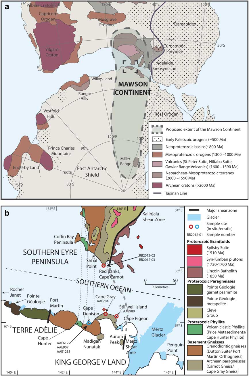
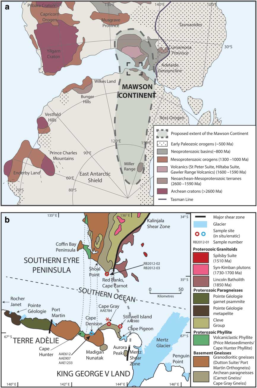
Reconstruction of the Mawson Continent. a. Reconstruction of Australia and Antarctica (after Fitzsimons Reference Fitzsimons2003, Payne et al. Reference Payne, Hand, Barovich, Reid and Evans2009, Reid & Hand Reference Reid and Hand2012). The Mawson Continent is comprised of the Gawler Craton (South Australia) and Terre Adélie–George V Coast (Antarctica). b. Correlation of lithologies between the southern Eyre Peninsula and Terre Adélie–George V Coast (after Fitzsimons Reference Fitzsimons2003, Ménot et al. Reference Ménot, Pecher, Rolland, Peucat, Pelletier, Duclaux and Guillot2005). In situ sample sites from this study are marked in red and erratic sample sites are marked in blue. Corresponding sample numbers for each site are indicated. Red asterisk represents the virtual position of the Red Banks Charnockite in this reconstruction.
Geological setting
The Mawson Continent rifted apart to produce Australian and Antarctic sections separated by the Southern Ocean commencing c. 83 Ma (Tikku & Cande Reference Tikku and Cande1999). Well-constrained palaeogeographical links between the Australian and Antarctic sections of the Mawson Continent during the Palaeoproterozoic are possible via the correlation of a narrow (c. 5 km wide) north–south trending belt of distinctive Mn-rich garnet–chlorite–magnetite phyllitic schist on the southern Eyre Peninsula in Australia (Price Metasediments) and at Cape Hunter along the George V Coast in Antarctica (Cape Hunter Phyllite; Fig. 1b). Both of these phyllitic lithologies have detrital zircon spectra indicating a unimodal population at c. 1765 Ma (Oliver & Fanning Reference Oliver and Fanning1997, Lane et al. Reference Lane, Jagodzinski, Dutch, Reid and Hand2015). Such precise geographical and geological correlation within the Mawson Continent implies that Cape Carnot and Red Banks in Australia are correlative with Cape Gray and surrounds in Antarctica (Fig. 1). For simplicity, events in the Mawson Continent will herein be described using the Gawler Craton terminology (i.e. Sleaford and Kimban).
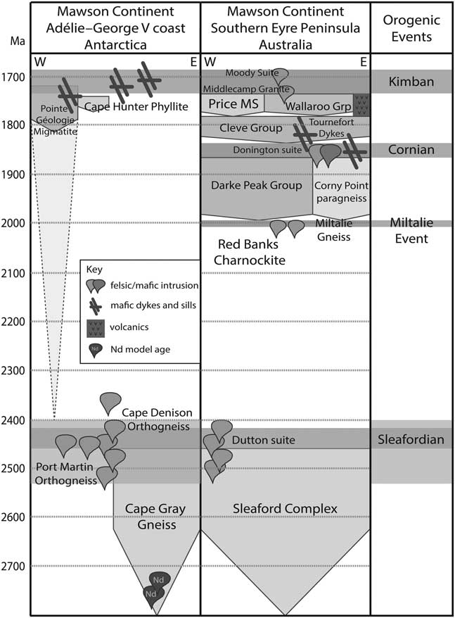
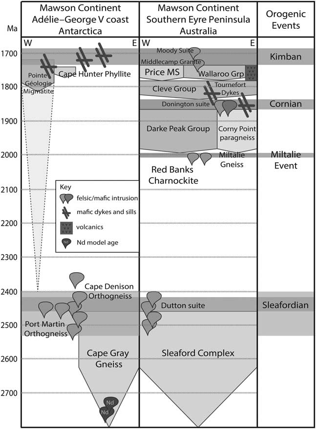
The Mawson Continent has a complex and prolonged tectonic history spanning 3200 Ma to 1500 Ma. Two protolith age domains have been identified in coastal outcrops of the Mawson Continent: Archean basement and overlying Palaeoproterozoic sequences (Fig. 1; e.g. Ménot et al. Reference Ménot, Pecher, Rolland, Peucat, Pelletier, Duclaux and Guillot2005, Di Vincenzo et al. Reference Di Vincenzo, Talarico and Kleinschmidt2007, Duclaux et al. Reference Duclaux, Rolland, Ruffet, Ménot, Guillot, Peucat, Fanning, Rey and Pêcher2008, Gapais et al. Reference Gapais, Pelletier, Ménot and Peucat2008). Palaeoarchaean (3400–3250 Ma) crust was reworked to form c. 3150 Ma granites, exposed in a narrow belt in the north-eastern Mawson Continent (Belousova et al. Reference Belousova, Reid, Griffin and O’Reilly2009). Meso–Neoarchaean basement is composed of orthogneiss, the protolith of which is 2800–2700 Ma (Nd model ages; Duclaux et al. Reference Duclaux, Rolland, Ruffet, Ménot, Guillot, Peucat, Fanning, Rey and Pêcher2008 and references therein) and subordinate paragneiss, such as the Sleaford Complex (Figs 1 & 2; Duclaux et al. Reference Duclaux, Rolland, Ruffet, Ménot, Guillot, Peucat, Fanning, Rey and Pêcher2008). Bimodal magmatism is recorded at 2560–2470 Ma (Hand et al. Reference Hand, Reid and Jagodzinski2007) and was terminated by deformation and metamorphism of the Sleaford event occurring at 2500–2400 Ma. The Sleaford event is characterized by metamorphic conditions that increase in grade from amphibolite facies in the west (5 kbar, 700–800°C; Ménot et al. Reference Ménot, Pecher, Rolland, Peucat, Pelletier, Duclaux and Guillot2005 and references therein, Hand et al. Reference Hand, Reid and Jagodzinski2007) to granulite facies in the east (7.5–10.5 kbar, 750–850°C; Ménot et al. Reference Ménot, Pecher, Rolland, Peucat, Pelletier, Duclaux and Guillot2005, Dutch et al. Reference Dutch, Hand and Kinny2008) between Port Martin/Coffin Bay Peninsula and the Mertz Glacier/Kalinjala Shear zone (Fig. 1; Ménot et al. Reference Ménot, Pecher, Rolland, Peucat, Pelletier, Duclaux and Guillot2005, Duclaux et al. Reference Duclaux, Rolland, Ruffet, Ménot, Guillot, Peucat, Fanning, Rey and Pêcher2008). The poorly understood Miltalie event involved c. 2010 Ma magmatism in a restricted belt in the eastern Mawson Continent (Hand et al. Reference Hand, Reid and Jagodzinski2007), including the 2011±7 Ma intrusion of the Red Banks Charnockite into the Carnot Gneiss/Cape Gray Gneiss (Fig. 2; Oliver & Fanning Reference Oliver and Fanning1997, Fitzsimons Reference Fitzsimons2003, Payne et al. Reference Payne, Hand, Barovich, Reid and Evans2009, Jagodzinski et al. Reference Jagodzinski, Reid and Hand2012). Following the Miltalie event, the tectonic regime was dominantly extensional and resulted in deposition of a series of sedimentary successions between 1850 and 1740 Ma (Szpunar et al. Reference Szpunar, Hand, Barovich, Jagodzinski and Belousova2011). Sedimentation was succeeded by the Kimban event at 1730–1690 Ma (Fig. 2) which generated high thermal gradient metamorphism widely across the Mawson Continent (Ménot et al. Reference Ménot, Pecher, Rolland, Peucat, Pelletier, Duclaux and Guillot2005, Hand et al. Reference Hand, Reid and Jagodzinski2007). Rocks of amphibolite–granulite facies grade from the Kimban event now dominate the exposed and known (via drill core) geology of the Mawson Continent. However, in places greenschist facies metamorphism is recorded at the surface, for example in the Cape Hunter Phyllite–Price Metasediments (Fig. 1; Ménot et al. Reference Ménot, Pecher, Rolland, Peucat, Pelletier, Duclaux and Guillot2005, Di Vincenzo et al. Reference Di Vincenzo, Talarico and Kleinschmidt2007). The Kimban event was inferred to have reworked the Palaeoproterozoic basins and Archean basement in a predominantly transpressional orogenic system (Ménot et al. Reference Ménot, Pecher, Rolland, Peucat, Pelletier, Duclaux and Guillot2005, Dutch et al. Reference Dutch, Hand and Kinny2008, Reference Dutch, Hand and Kelsey2010). Although the Kimban event is widely reported from the Mawson Continent, it has an uncertain spatial extent at the outcrop to kilometre scale, with different studies arguing either for local metamorphic resetting related to deformation along discrete shear zones (Oliver & Fanning Reference Oliver and Fanning2002, Duclaux et al. Reference Duclaux, Rolland, Ruffet, Ménot, Guillot, Peucat, Fanning, Rey and Pêcher2008, Gapais et al. Reference Gapais, Pelletier, Ménot and Peucat2008) or regionally pervasive overprinting that completely overprinted any older record (Di Vincenzo et al. Reference Di Vincenzo, Talarico and Kleinschmidt2007). The 1620–1570 Ma interval was dominated by magmatism, including the c. 1620 Ma St Peter Suite, the c. 1600 Ma volcanics at Rocher Janet and the c. 1590 Ma Hiltaba suite and coeval Gawler Range Volcanics (Fig. 1; Hand et al. Reference Hand, Reid and Jagodzinski2007, Gapais et al. Reference Gapais, Pelletier, Ménot and Peucat2008 and references therein). The Mawson Continent was not reworked by the later c. 500 Ma Delamerian–Ross Orogeny, which is pervasive to the east of the Mertz Shear Zone/Tasman Line (Fig. 1; Gapais et al. Reference Gapais, Pelletier, Ménot and Peucat2008).
Time–space plot of the Mawson Continent, divided into the Antarctic Mawson Continent and Australian Mawson Continent sections (after Fitzsimons Reference Fitzsimons2003, Payne et al. Reference Payne, Hand, Barovich, Reid and Evans2009, Dutch et al. Reference Dutch, Hand and Kelsey2010; additional data are included from Oliver & Fanning Reference Oliver and Fanning1997, Ménot et al. Reference Ménot, Pecher, Rolland, Peucat, Pelletier, Duclaux and Guillot2005, Duclaux et al. Reference Duclaux, Rolland, Ruffet, Ménot, Guillot, Peucat, Fanning, Rey and Pêcher2008, Gapais et al. Reference Gapais, Pelletier, Ménot and Peucat2008, Szpunar et al. Reference Szpunar, Hand, Barovich, Jagodzinski and Belousova2011, Jagodzinski et al. Reference Jagodzinski, Reid and Hand2012). Grp=Group, MS=metasediments.
The record of the Kimban and Sleaford events is difficult to distinguish at scales from centimetres to tens of kilometres. One of the difficulties in distinguishing the two events (and polymetamorphism in general) is that polymetamorphism is easily recognizable only where zones of structural reworking correspond to clear differences in metamorphic grade. A common example is mica-rich shear zones dissecting largely anhydrous granulites (e.g. Raimondo et al. Reference Raimondo, Clark, Hand, Cliff and Anczkiewicz2013). However, recognizing polymetamorphism is far more challenging where i) metamorphic grade of superimposed events is similar and regionally distributed without apparent demarcation, and ii) the orientation of tectonic fabrics are subparallel. In such cases, reworking and polymetamorphism is most effectively identified through application of geochronology, as the petrological and geochemical record of reworking may only be manifest as subtle differences in mineral assemblages and/or mineral chemistry (e.g. Kelsey et al. Reference Kelsey, Hand, Clark and Wilson2007, Diener et al. Reference Diener, White and Powell2008, Mahan et al. Reference Mahan, Smit, Williams, Dumond and van Reenen2011, Korhonen et al. Reference Korhonen, Clark, Brown, Bhattacharya and Taylor2013, Morrissey et al. Reference Morrissey, Hand, Kelsey and Wade2016). Partly due to this complexity in polyphase high-grade rocks, the P–T conditions of the Kimban event versus the Sleaford event in the southern Eyre Peninsula–George V Coast of the Mawson Continent have yet to be systematically constrained.
Sample selection and petrography
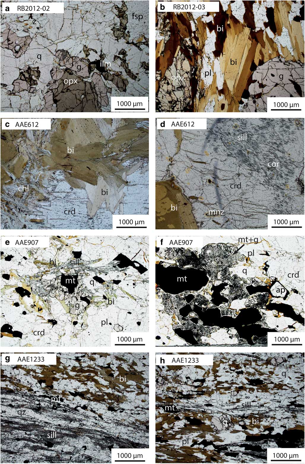
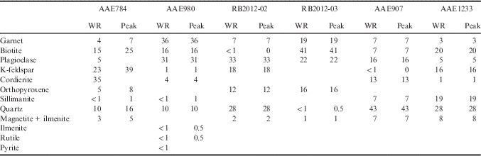
The samples chosen for petrolographic analysis, phase equilibria modelling and geochronology were from five locations in the Mawson Continent. In situ samples were located at Cape Gray and Stillwell Island (George V Coast) and Red Banks (southern Eyre Peninsula; Fig. 1b, Table I). Erratic samples were from glacial moraines located at Cape Denison (Fig. 1b). Samples prefixed by ‘AAE’ are legacy samples from Sir Douglas Mawson’s 1911–1914 AAE. Field and hand sample photographs for all samples are provided in Fig. 3, and photomicrographs of thin sections are shown in Figs 4 & 5. Samples are described in detail below and modal abundance estimates for minerals are given in Table II. Mineral modal abundance (vol%) estimates with errors were derived using the average of estimates made by five independent persons, and the 1σ standard deviation between them. Mineral proportions of feldspars, cordierite and quartz were estimated using a mass balance approach incorporating bulk-rock chemistry and electron microprobe data (Table S1 & Appendix S2 found at http://dx.doi.org/10.1017/S0954102017000451).
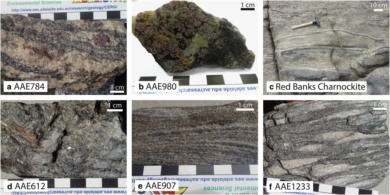
Hand sample and field photographs. a. In situ sample AAE784 from Cape Gray, migmatitic garnet–cordierite gneiss. b. In situ sample AAE980 from Stillwell Island, garnet–plagioclase–cordierite–biotite gneiss. c. Red Banks Charnockite, migmatized orthopyroxene–garnet–biotite gneiss. d. Erratic sample AAE612 from Cape Denison, biotite–chlorite–cordierite–sillimanite gneiss. e. Erratic sample AAE907 from Cape Denison, garnet–cordierite–sillimanite gneiss. f. Erratic sample AAE1233 from Cape Denison, sillimanite–biotite gneiss.

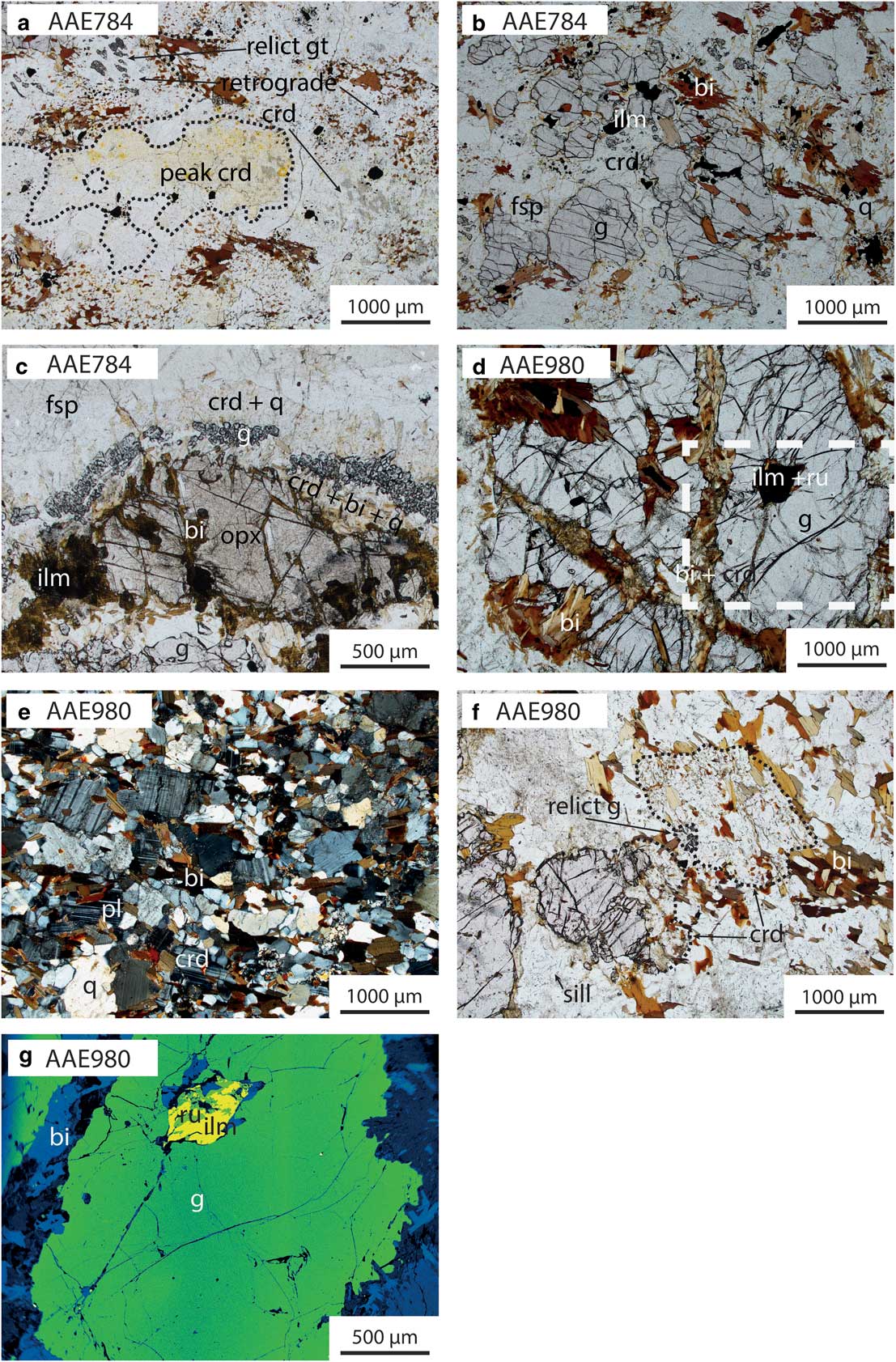
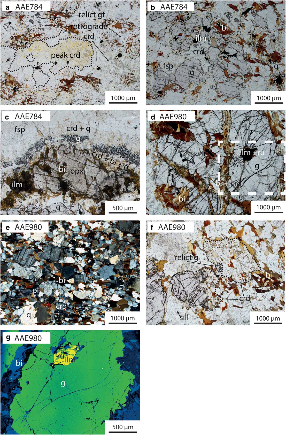
Photomicrographs of key petrological relationships in Antarctic coastal samples. Photomicrographs are taken in plane polarized light unless specified. Dashed black lines indicate grain or pseudomorph boundaries. a. AAE784: peak cordierite contains inclusions of ilmenite + sillimanite + monazite only, retrograde cordierite contains relict garnet and biotite inclusions. b. AAE784: relict garnet surrounded by late cordierite. c. AAE784: multilayer corona separating coarse grained orthopyroxene + garnet from K-feldspar + plagioclase. From the orthopyroxene to the feldspars the layers of the corona are: i) biotite + cordierite + quartz, ii) garnet, + quartz and iii) symplectic cordierite + quartz. d. AAE980: garnet porphyroblast with ilmenite inclusions and late biotite ± cordierite (see g. for inset). e. AAE980: cross-polarized light: matrix of biotite + plagioclase + cordierite + quartz. f. AAE980: cordierite patches adjacent to relict garnet. Fibrous sillimanite included in plagioclase. g. AAE980: false colour backscatter electron image; inclusion of rutile and ilmenite in garnet. bi=biotite, crd=cordierite, fsp=feldspar, g=garnet, ilm=ilmenite, opx=orthopyroxene, pl=plagioclase, q=quartz, ru=rutile, sill=sillimanite.
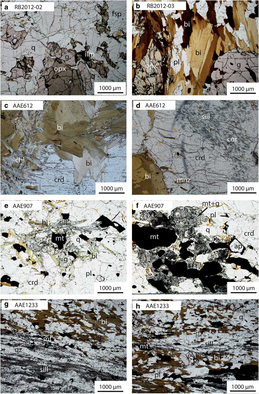
Photomicrographs of key petrological relationships in the Red Banks Charnockite and Antarctic erratic samples. Photomicrographs are taken in plane polarized light. a. RB2012-02: coarse grained garnet grows around coarse grained orthopyroxene in a matrix of plagioclase + K-feldspar + quartz. b. RB2012-03: coarse grained biotite defines foliation, in contact with coarse grained orthopyroxene and porphyroblastic garnet. c. AAE612: coarse grained cordierite + biotite + chlorite. d. AAE612: corundum and sillimanite in cordierite. e. AAE907: coarse grained magnetite + garnet + sillimanite + biotite + plagioclase + cordierite. f. AAE907: coarse grained magnetite, quartz and plagioclase separated by fine grained garnet–magnetite symplectites. g. AAE1233: contact between domains dominated by coarse grained biotite (top right) and sillimanite (bottom left). h. AAE1233: garnet + ilmenite + sillimanite within biotite domain. ap=apatite, bi=biotite, chl=chlorite, crd=cordierite, , cor=corundum, fsp=feldspar, g=garnet, ilm=ilmenite, mnz=monazite, mt=magnetite, opx=orthopyroxene, pl=plagioclase, q=quartz, sill=sillimanite.
Summary of sample locations and analytical datasets. Mineral abbreviations after Holland & Powell (Reference Holland and Powell1998).

bi=biotite, chl=chlorite, cor=corundum, crd=cordierite, EPMA=electron probe microanalysis, g=garnet, ilm=ilmenite, ksp=K-feldspar, mt=magnetite, opx=orthopyroxene, pl=plagioclase, q=quartz, ru=rutile, sill=sillimanite.
Summary of mineral modal abundances for samples used in forward phase equilibria modelling. All values are in %.
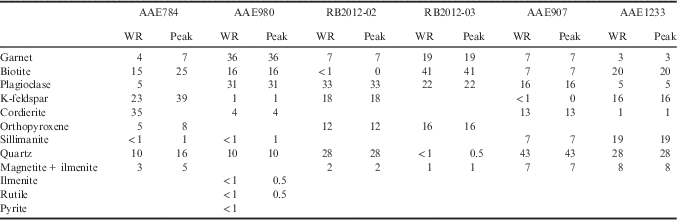
WR=whole rock mineral modes from sample.
Peak=normalized peak mineral assemblage modes (to 100%).
AAE784 (Cape Gray Gneiss, in situ)
At the mesoscopic scale, this sample is coarse grained and contains light and dark coloured layers (Fig. 3a). The light coloured layers dominantly comprise K-feldspar and plagioclase but also contain elongated garnet porphyroblasts ≤10 mm in length and rare porphyroblasts of orthopyroxene. The darker coloured parts of the rock are primarily composed of biotite, cordierite and garnet.
In thin section within the darker coloured layers, garnet is ≤1 mm diameter but has poor crystal habit with deeply embayed grain boundaries. Biotite occurs as coarse grained (≤4 mm) relicts within patches containing abundant fine grained (0.1 mm) aggregates of biotite and cordierite. These aggregates commonly contain abundant inclusions of magnetite ± ilmenite ± garnet ± sillimanite (Fig. 4a), and consistently separate garnet from coarse grained biotite and K-feldspar (Fig. 4a & b). Rare cordierite aggregates contain only inclusions of ilmenite and monazite (Fig. 4a). Magnetite and ilmenite occur distributed throughout the sample as anhedral grains ≤0.5 mm, commonly in contact with biotite (Fig. 4b).
A K-feldspar-rich layer in the sample comprises 10% of the thin section and corresponds to the lighter coloured layers in the hand specimen. This layer contains coarse grained orthopyroxene (4 mm), garnet (3 mm), perthitic K-feldspar and plagioclase. Plagioclase occurs only as rims on K-feldspar, thus is interpreted to be post-peak in origin. In this domain, a multilayered corona systematically separates orthopyroxene and garnet from K-feldspar and plagioclase. From the orthopyroxene to the feldspars, the layers of the corona (Fig. 4c) are: i) acicular biotite, which grows approximately radially outward from the orthopyroxene and occurs with cordierite and quartz, ii) fine grained garnet forming an aggregated layer with 5% quartz, and iii) symplectic intergrowth between cordierite and quartz.
As this sample is from the AAE legacy collection, understanding of the original field relationships is incomplete. However, the orthopyroxene–K-feldspar-bearing layer has been interpreted as a leucosome in a garnet–cordierite–biotite-bearing gneiss. Therefore, the prograde-to-peak assemblage is interpreted to contain sillimanite and garnet, the peak assemblage to be garnet–orthopyroxene–K-feldspar–cordierite–magnetite–ilmenite–quartz–melt and the post-peak assemblage to involve development of cordierite, plagioclase and biotite ± garnet. The multilayer corona mantling orthopyroxene is interpreted as post-peak in origin.
AAE980 (Stillwell Island metapelite, in situ)
At the mesoscopic scale, the sample is gneissic. It contains coarse grained garnet (≤20 mm), that can occur as aggregates ≤30 mm in diameter, amongst coarse grained (≤3 mm) plagioclase and biotite (≤4 mm; Fig. 3b). Garnet-poor areas are dark coloured and contain finer grained (>1 mm) biotite, finer grained (4 mm) garnet and light coloured minerals (quartz, feldspar). This part of the rock contains a weak foliation defined by biotite.
In thin section, the coarse grained garnet accompanied by plagioclase, biotite, and minor quartz and ilmenite. Biotite is unoriented and occurs as inclusions ≤2 mm in diameter in garnet, between porphyroblasts of garnet as well as in fractures in garnet (Fig. 4d). In the garnet-poor areas of the sample, the mineralogy is biotite, plagioclase, garnet, cordierite, ilmenite, sillimanite, quartz and accessory K-feldspar (Fig. 4e & f). Cordierite occurs as anhedral grains with inclusions of rare sillimanite (Fig. 4e). Garnet with embayed grain boundaries is commonly surrounded by patches of cordierite and unoriented biotite (Fig. 4f). Rare sillimanite occurs as unoriented acicular grains ≤0.5 mm in length in plagioclase and cordierite and as rare inclusions in garnet (Fig. 4e). Rare K-feldspar grains occur in contact with coarse grained biotite and plagioclase. Ilmenite and pyrite occur as inclusions in garnet, with ilmenite rarely intergrown with fine grained rutile (Fig. 4g), and all three are consistently separated from garnet by biotite ± cordierite. Ilmenite additionally occurs throughout the sample, whereas rutile and pyrite only occur as inclusions in garnet.
Considering the grain size and mineralogy of the two parts of the rock, the coarse garnet–plagioclase part of the rock is interpreted as a coarse grained leucosome and the finer grained biotite–garnet–cordierite part of the rock represents melanosome. The rutile and sillimanite inclusions in garnet and plagioclase are interpreted to have developed prior to the peak metamorphic assemblage. The interpreted peak assemblage is garnet–plagioclase–biotite–ilmenite–quartz–melt ± cordierite ± sillimanite and post-peak mineral development involved the growth of cordierite and biotite at the expense of garnet±sillimanite. The abundance of late, relatively coarse grained biotite may indicate the former presence of trapped melt.
Red Banks Charnockite (Red Banks, in situ)
Jagodzinski et al. (Reference Jagodzinski, Reid and Hand2012) previously described the Red Banks Charnockite as an orthopyroxene-bearing gneiss. The c. 2010 Ma bimodal felsic and mafic protolith to the charnockite intruded a c. 2450 Ma metasedimentary granulite comprising part of the Sleaford Complex (Jagodzinski et al. Reference Jagodzinski, Reid and Hand2012). At the outcrop scale, the rock structure is entirely metamorphic; i.e. the gneiss is heterogeneous and migmatitic with centimetre-scale zones of homogeneous mineralogy (Fig. 3c). Leucosomes are abundant (c. 50% of area of outcrop) and comprise primarily K-feldspar and plagioclase. Melanosomes contain biotite±garnet ± orthopyroxene. The foliation is defined by biotite and orthopyroxene, with orthopyroxene also occurring in cross-cutting leucocratic/migmatitic segregations. Two samples collected from within c. 1 m2 of outcrop are described below.
RB2012-02 (Red Banks, in situ)
This sample has a weak foliation, defined by coarse grained (≤6 mm) orthopyroxene. Medium grained (≤1 mm) K-feldspar, plagioclase and quartz form the matrix, which comprises 70% of the sample. Garnet and orthopyroxene occur in direct contact (Fig. 5a). Minor magnetite and ilmenite occur with accessory biotite. The interpreted peak assemblage is garnet–orthopyroxene–K-feldspar–plagioclase–magnetite–ilmenite–quartz–melt.
RB2012-03 (Red Banks, in situ)
RB2012-03 is coarser grained than RB2012-02. The sample contains a fabric defined by biotite grains ≤5 mm in length and elongate grains of orthopyroxene ≤15 mm long and 5 mm (Fig. 5b, Table II). Subhedral to euhedral, poikiloblastic garnet ≤8 mm in diameter contains inclusions of quartz, plagioclase and biotite. Garnet commonly occurs in contact with biotite and less commonly in contact with orthopyroxene. Coarse to medium grained plagioclase and minor quartz occur interstitially amongst biotite. Minor magnetite and ilmenite occur in contact with the coarse grained minerals. The interpreted peak assemblage is biotite–garnet–orthopyroxene–plagioclase–ilmenite–magnetite–melt ± quartz. The quartz was interpreted as part of the peak assemblage; however, the petrolographic significance of quartz in rocks with low quartz content is typically ambiguous (e.g. Waters Reference Waters2001) and it is therefore difficult to unequivocally determine whether quartz forms part of the peak assemblage in this sample.
AAE612 (Cape Denison, erratic)
At the mesoscopic scale, this sample is primarily composed of coarse grained cordierite, biotite and chlorite (Fig. 3d). In thin section, coarse grained subhedral cordierite (≤10 mm), biotite (grains ≤10 mm in length, aggregates ≤40 mm) and chlorite (grains ≤10 mm and aggregates ≤30 mm) together comprise 95% by area of the sample. Biotite and chlorite commonly occur as mass aggregates of a single mineral, but may be intergrown and define a weak foliation. Cordierite contains randomly oriented inclusions of biotite ≤5 mm in length. The sample also contains small, rare patches consisting of sillimanite and corundum with accessory rutile, separated from each other by fine grained cordierite (Fig. 5c & d). These patches are also separated from biotite and chlorite by cordierite (Fig. 5d). Sillimanite and corundum in these zones occur as fine grained aggregates and are strongly oriented with fibrous sillimanite and tabular corundum aligned approximately parallel to the foliation in the sample. Cordierite ± chlorite is interpreted to be mostly the product of post-peak metamorphic evolution. The peak assemblage is difficult to discern but may comprise corundum–sillimanite–biotite ± chlorite ± cordierite.
AAE907 (Cape Denison, erratic)
At the mesoscopic scale, this sample is gneissic, with layers c. 4 mm thick. Dark coloured layers are composed of magnetite, garnet, sillimanite and minor quartz and light coloured layers are composed of plagioclase, cordierite, sillimanite, quartz, minor biotite and accessory K-feldspar (Fig. 3e). As the alternation of layers is regular, the rock is effectually homogeneous at the scale of the hand specimen and thin section. In thin section within the light coloured layers, coarse grained magnetite (≤3 mm in size) occurs in contact with coarse grained cordierite and quartz (each ≤2 mm). Cordierite contains fine grained inclusions of magnetite and ilmenite (Fig. 5e). In the dark coloured layers, coarse grained magnetite occurs in direct contact with fine grained intergrowths of magnetite and garnet (Fig. 5f) that are spatially restricted to areas with low abundance of sillimanite and biotite. Magnetite also occurs with aggregates of subhedral garnet, biotite and acicular to blocky sillimanite ± chlorite. The mineral assemblage in this sample is consistent with formation in the presence of melt. The interpreted peak assemblage is magnetite–garnet–plagioclase–cordierite–sillimanite–biotite–ilmenite–quartz–melt with biotite and garnet–magnetite symplectites interpreted as post-peak minerals.
AAE1233 (Cape Denison, erratic)
This sample is strongly layered at the mesoscopic scale, defined by alternating aggregates of sillimanite (≤2 mm wide and 10 mm long) and biotite (Figs 3f & 5g). In thin section, coarse grained biotite (≤3 mm long) is anhedral to subhedral. Garnet (≤2 mm in diameter) is subhedral, inclusion-free and occurs more commonly in biotite-rich layers (Fig. 5h). Evenly distributed ilmenite and magnetite are ≤4 mm in size within the biotite-bearing layers. Quartz, K-feldspar, plagioclase and minor cordierite comprise 50% of the sample and rarely contain randomly oriented, acicular sillimanite grains. Rare accessory tourmaline grains (≤2 mm in size) occur in contact with coarse grained sillimanite, biotite, ilmenite and quartz. The interpreted peak assemblage is magnetite–sillimanite–biotite–garnet–ilmenite–K-feldspar–plagioclase–cordierite–quartz.
Methods
Monazite geochronology
U-Pb monazite geochronology was obtained by laser ablation–inductively coupled–mass spectrometry (LA–ICP–MS) for in situ samples AAE784, AAE980 and RB2012-02, and for erratic samples AAE612, AAE907 and AAE1233. Analytical techniques for in situ U-Pb isotopic dating of monazite follow those of Payne et al. (Reference Payne, Hand, Barovich and Wade2008). Prior to U-Pb analysis, monazites were imaged with a backscatter electron (BSE) detector in thin section using a Phillips XL-30 Field emission scanning electron microscope at the University of Adelaide. U-Pb isotopic analyses were obtained using a New Wave 213 nm Nd–YAG laser in an He ablation atmosphere, coupled to an Agilent 7500cs/7500s ICP–MS at the University of Adelaide. Ablation of monazites was performed in situ with a beam diameter of 15 µm and repetition rate of 5 Hz, with a total acquisition time of 80 s, comprising 30 s of background measurement, 10 s for beam and crystal stabilization, and 40 s of sample ablation. Isotopes 204Pb, 206Pb, 207Pb and 238U were measured for dwell times of 10, 15, 30 and 15 ms, respectively. U-Pb fractionation was corrected using the MAdel monazite standard (TIMS normalization data: 207Pb/206Pb age=490.7 Ma, 206Pb/238U age=514.8 Ma, 207Pb/235U age=510.4 Ma; Payne et al. Reference Payne, Hand, Barovich and Wade2008), with an overestimated absolute uncertainty of 1% assigned to each normalization age. Accuracy was also monitored by repeat analyses of the in-house internal standard 94-222/Bruna-NW (c. 450 Ma; Payne et al. Reference Payne, Hand, Barovich and Wade2008) and data reduction was completed using GLITTER software (Jackson et al. Reference Jackson, Pearson, Griffin and Belousova2004). Over the duration of this study, the reproducibility (external precision) of the MAdel standard was ± 2.2 Ma for 207Pb/206Pb,±0.79 Ma for 206Pb/238U, and ± 0.67 Ma for 207Pb/235U (2σ; n=145). The weighted average ages for 94-222/Bruna-NW were 453.1±3.1 Ma for 207Pb/206Pb, 451.2±2.1 Ma for 206Pb/238U and 451.2±1.7 Ma for 207Pb/235U (95% confidence; n=82).
Common Pb could not be explicitly measured because of the unresolvable interference of 204Hg on 204Pb. Uncorrected isotope ratios are thus used for all age calculations, with concordia plots and upper intercept ages generated using Isoplot/Ex 3.71 (Ludwig Reference Ludwig2008). Weighted average age calculations (reported at 95% confidence) were also performed using uncorrected 207Pb/206Pb ratios.
Bulk-rock chemistry
Whole rock geochemical analyses used for phase equilibria forward modelling were undertaken by wavelength dispersive X-ray fluorescence spectrometry at the Department of Earth and Environment, Franklin and Marshall College, Lancaster, PA, USA. Major elements were analysed on fused disks prepared using a lithium tetraborate flux. Whole rock geochemical analyses are presented in Table S1.
Phase equilibria modelling
Phase equilibria forward models for samples AAE784, AAE980, RB2012-02, RB2012-03, AAE907 and AAE1233 were calculated using the software program THERMOCALC v.3.40 with the latest internally consistent thermodynamic dataset, tc-ds62.txt (Holland & Powell Reference Holland and Powell2011). Forward modelling for sample AAE612 was not performed because of the presence of the compositional and mineralogical domains occurring in this refractory sample. Forward models were calculated for the geologically realistic system of MnNCKFMASHTO (MnO–Na2O–CaO–K2O–FeO–MgO–Al2O3–SiO2–H2O–TiO2–Fe2O3). The activity–composition (a–x) models from White et al. (Reference White, Powell, Holland, Johnson and Green2014b) were used, reparameterized for the Mn-bearing system (Powell et al. Reference Powell, White, Green, Holland and Diener2014, White et al. Reference White, Powell and Johnson2014a). The FeO:Fe2O3 ratio and H2O content of each sample was constrained using calculated T–M O and T–M H2O models, respectively (Appendix S3 found at http://dx.doi.org/10.1017/S0954102017000451).
Phase equilibria forward models were contoured for normalized abundances (‘modes’) of phases using the Matlab-based automated program TCInvestigator v 2.0 (Pearce et al. Reference Pearce, White and Gazley2015) for T–M and P–T models. Calculated contours for peak mineral modes were used in conjunction with observed mineral abundances to constrain P–T conditions within the peak assemblage field.
Results
Monazite geochronology
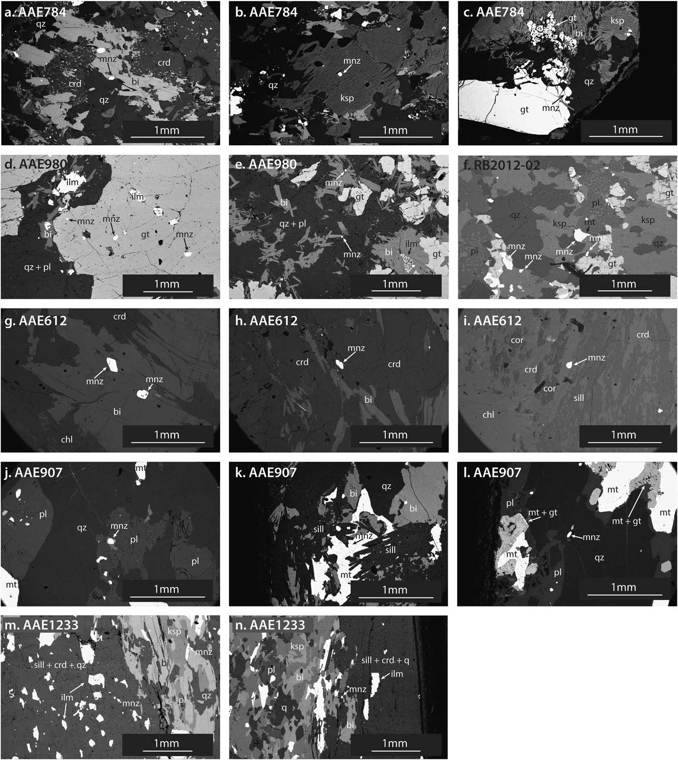
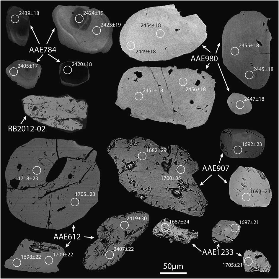
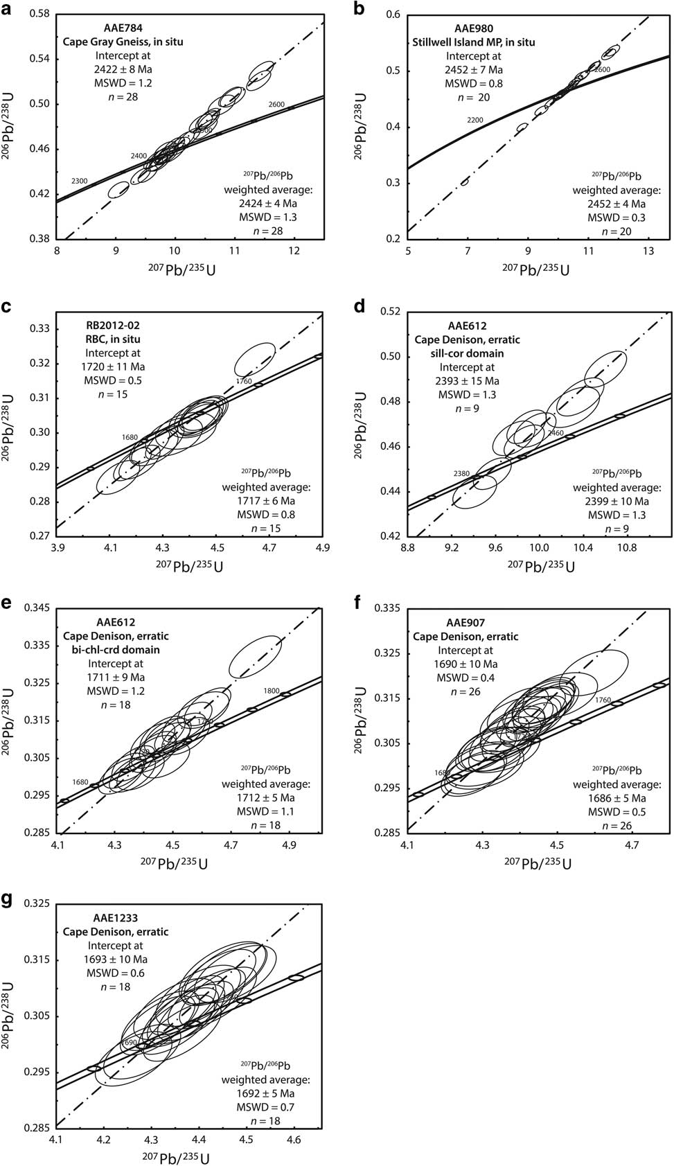
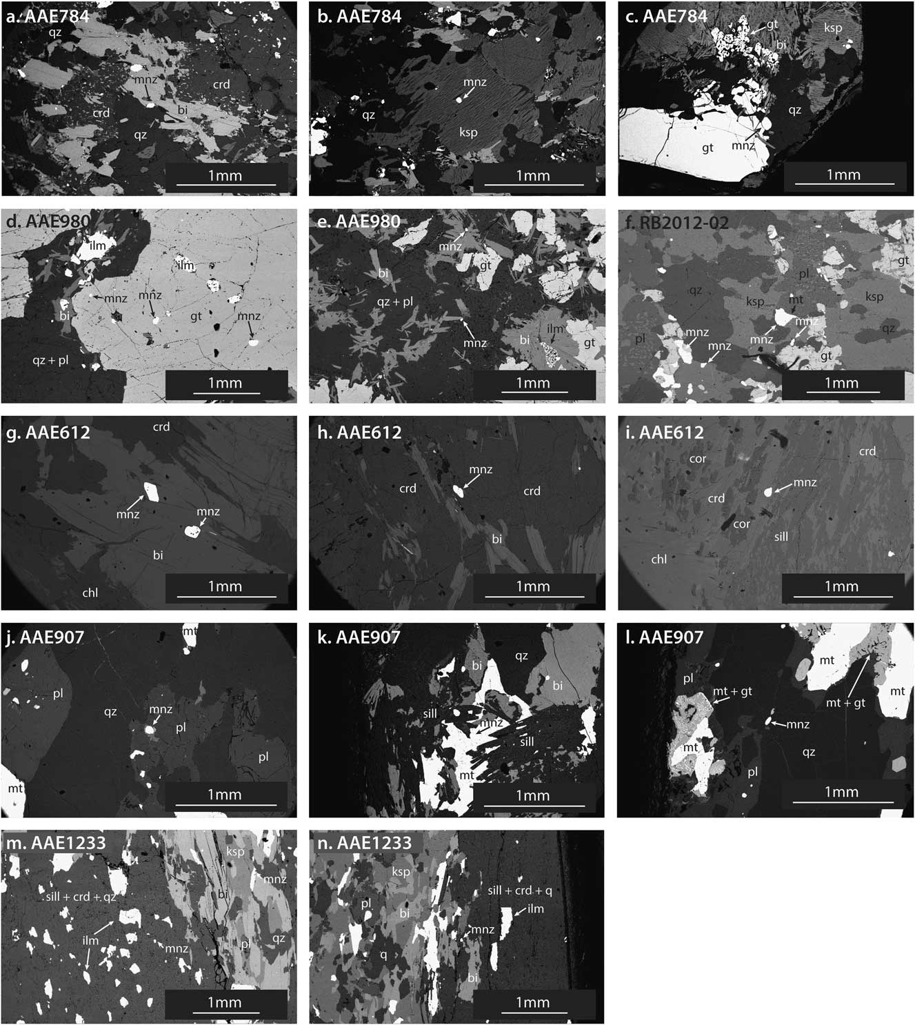
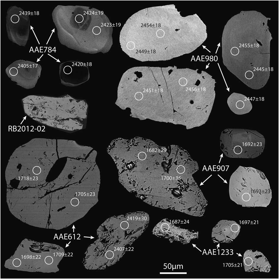
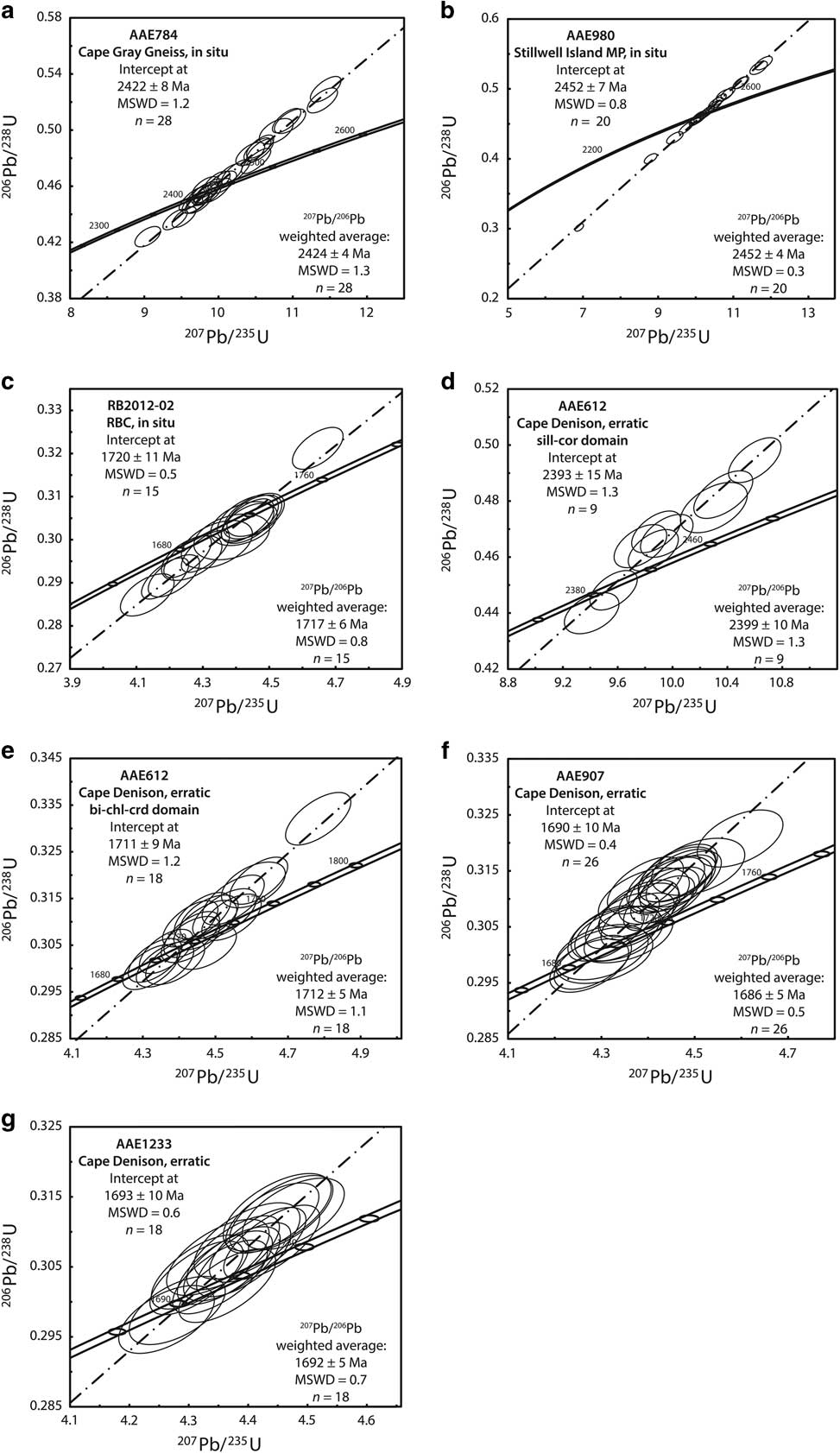
All geochronological data are provided in Table S4 (found at http://dx.doi.org/10.1017/S0954102017000451) and summarized in Table I. The BSE images of textural relations and individual monazite grains are provided in Figs 6 & 7, respectively, and concordia plots are provided in Fig. 8.
Backscatter electron images indicating microstructural positions of monazite grains used for in situ LA–ICP–MS U-Pb geochronology. a. AAE784: monazite included in matrix biotite. b. AAE784: monazite included in coarse grained feldspar. c. AAE784: monazite in contact with coarse grained garnet in K-feldspar-rich zone. d. AAE980: monazite included in garnet porphyroblasts. e. AAE980: monazite in contact with biotite in matrix. f. RB2012-02: monazite distributed throughout coarse grained assemblage. g. AAE612: monazite included in biotite in matrix. h. AAE612: monazite included in cordierite in matrix. i. AAE612: monazite in sillimanite–corundum patch. j. AAE907: monazite in light coloured layer, included in plagioclase. k. AAE907: monazite included in sillimanite. l. AAE907: monazite included in quartz adjacent to magnetite–garnet symplectites. m. AAE1233: monazite in matrix in light coloured layer. n. AAE1233: monazite in matrix in dark coloured layer.
Backscatter electron images of individual monazite grains showing internal morphology. Circles representing LA–ICP–MS analyses are 15 µm in diameter and labelled with 207Pb/206Pb ages (Ma). Sample AAE784 shows broad, simple core–rim zoning. Samples AAE980, AAE907 and AAE1233 show subtle indistinct zoning. Samples RB2012-02 and AAE612 are unzoned.
Concordia plots and calculated age estimates for in situ LA–ICP–MS monazite U-Pb data. All age uncertainties are quoted at the 95% confidence level. 207Pb/206Pb weighted average age calculations are also included for each sample. Abbreviations: bi=biotite, chl=chlorite, crd=cordierite, cor=corundum, MP=metapelite, MSWD=mean square of weighted deviates, RBC=Red Banks Charnockite, sill=sillimanite.
All samples in this study show unimodal age populations, with the exception of sample AAE612, which records two distinct age peaks. The microstructural location of monazite in a given sample does not appear to play any role in the distribution of ages, with the exception of sample AAE612 (Fig. 6). Individual monazite grains in sample AAE612 all show unimodal age peaks, with little internal variation within grains. However, there is a clear relationship between age data and the microstructural location of monazite. Monazite with Sleaford ages (c. 2400 Ma) is located in sillimanite–corundum bearing domains, whereas monazite with Kimban ages (c. 1710 Ma) is located in cordierite–biotite–chlorite domains. For all other samples contrasting zonation features in monazite were targeted where possible (size permitting), but no systematic age variation was observed for multiple analyses on single grains.
All samples include reversely discordant analyses but have a higher proportion of concordant or near concordant analyses. Furthermore, the 207Pb/206Pb weighted average age and concordia-intercept age for each sample are indistinguishable within error, suggesting that the reverse discordance has not affected the age accuracy. Sample AAE980 shows a larger spread of normally discordant analyses than other samples in this study, most probably indicating recent Pb loss. However, these analyses lie on the regression line that again agrees with the 207Pb/206Pb weighted average age and hence are not considered as outliers.
For sample AAE784, 28 analyses were obtained from 26 individual monazite grains hosted by biotite, K-feldspar and at quartz–garnet grain boundaries (Fig. 6a–c). Monazite grains show distinct core–mantle internal zoning (Fig. 7). The data record an age spread of 2450–2399 Ma (Fig. 8a). The 207Pb/206Pb weighted average age is 2424±4 Ma (n=28, mean square of weighted deviates (MSWD)=1.3), which is within error of the upper intercept age of 2422±8 Ma (n=28, MSWD=1.2).
For sample AAE980, 20 analyses were obtained from 17 individual monazite grains hosted by garnet and at biotite–plagioclase grain boundaries (Fig. 6d & e). Monazite grains show subtle indistinct zoning (Fig. 7). The data record an age spread of 2470–2445 Ma (Fig. 8b). The 207Pb/206Pb weighted average age is 2452±4 Ma (n=20, MSWD=0.3), which is within error of the upper intercept age of 2452±7 (n=20, MSWD=0.8).
For sample RB2012-02, 15 analyses were obtained from 14 individual monazite grains hosted at grain boundaries between garnet, K-feldspar, magnetite and quartz (Fig. 6f). Monazite grains are devoid of internal zoning (Fig. 7). The data record an age spread of 1731–1701 Ma (Fig. 8c). The 207Pb/206Pb weighted average age is 1717±6 Ma (n=15, MSWD=0.8), which is within error of the upper intercept age of 1720±11 Ma (n=15, MSWD=0.5).
For sample AAE612, 27 analyses were obtained from nine individual monazite grains in two distinct microstructural settings: monazite hosted by biotite and cordierite in the cordierite–biotite–chlorite domain of the rock, and monazite hosted by cordierite in the sillimanite–corundum-bearing domain (Fig. 6g–i). Monazite grains from both domains are devoid of internal zoning (Fig. 7). The data record two distinct age populations. The older population (sillimanite–corundum-bearing domain; Fig. 8d) gives a weighted average 207Pb/206Pb age of 2399±10 Ma (n=9, MSWD=1.3), which is within error of the upper intercept age of 2393±15 Ma (n=9, MSWD=1.3). The younger population (biotite–chlorite–cordierite-bearing domain; Fig. 8e) gives a weighted average 207Pb/206Pb age of 1712±5 Ma (n=18, MSWD=1.1), which is within error of the upper intercept age of 1711±9 Ma (n=18, MSWD=1.2).
For sample AAE907, 26 analyses were obtained from 20 individual monazite grains hosted by plagioclase, magnetite and quartz (Fig. 6j–l). Monazite grains show subtle indistinct zoning (Fig. 7). The data record an age spread of 1700–1662 Ma (Fig. 8f). The 207Pb/206Pb weighted average age is 1686±5 Ma (n=26, MSWD=0.5), which is within error of the upper intercept age of 1690±10 Ma (n=26, MSWD=0.4).
For sample AAE1233, 18 analyses were obtained from 12 individual monazite grains hosted by cordierite, quartz and at K-feldspar–biotite–magnetite grain boundaries (Fig. 6m & n). Monazite grains show subtle indistinct zoning (Fig. 7). The data record an age spread of 1711–1678 Ma (Fig. 8g). The 207Pb/206Pb weighted average age is 1692±5 Ma (n=18, MSWD=0.7), which is within error of the upper intercept age of 1693±10 Ma (n=18, MSWD=0.6).
P–T conditions
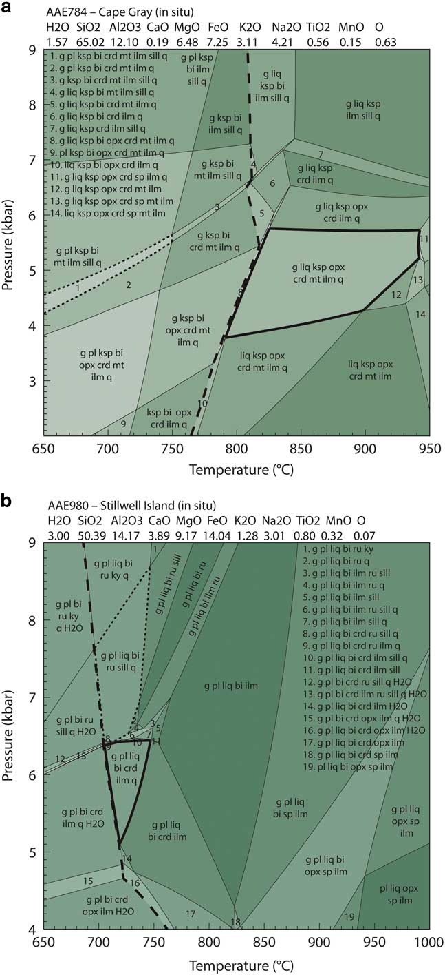
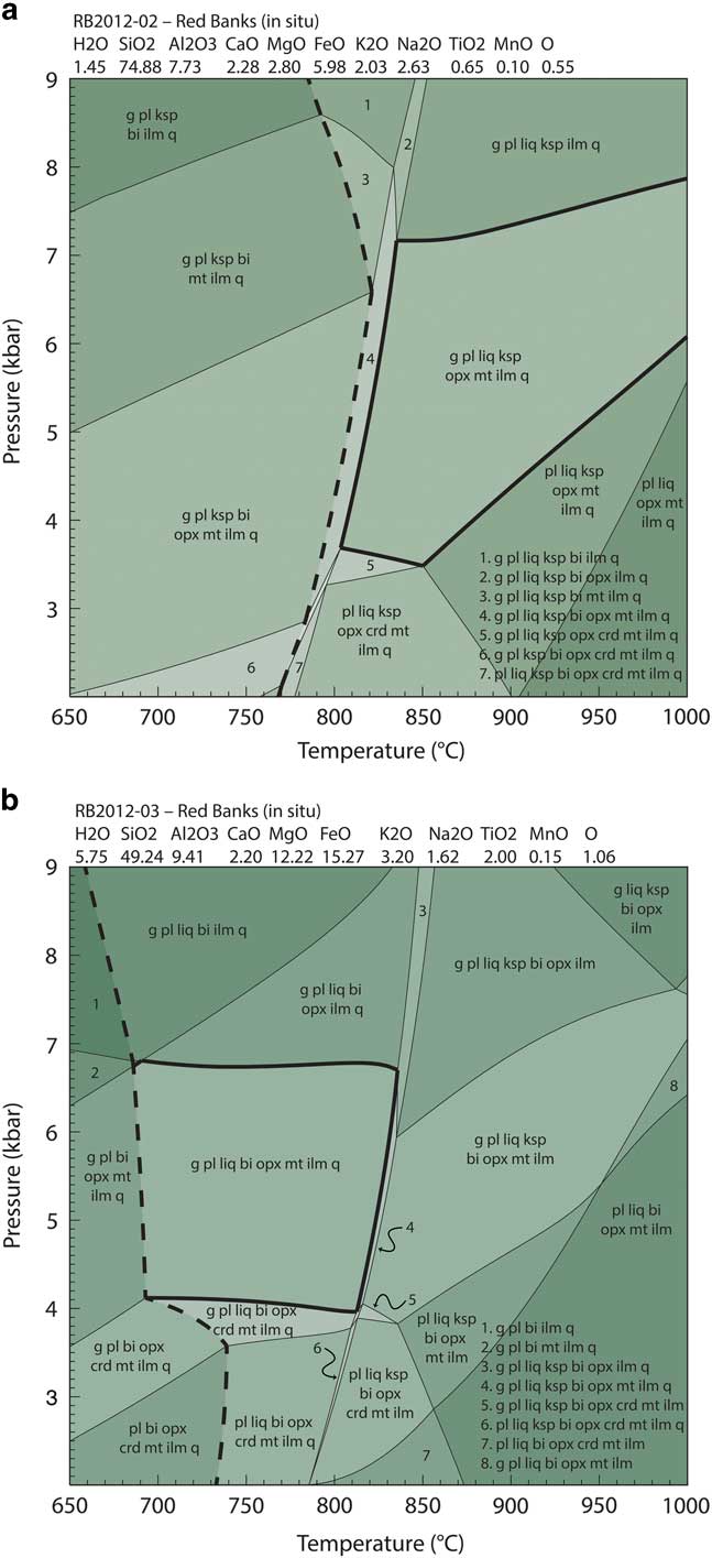
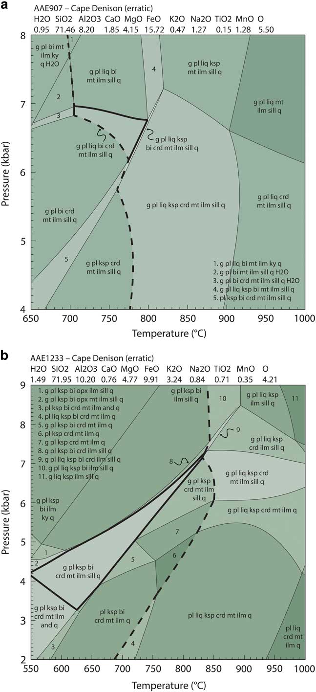
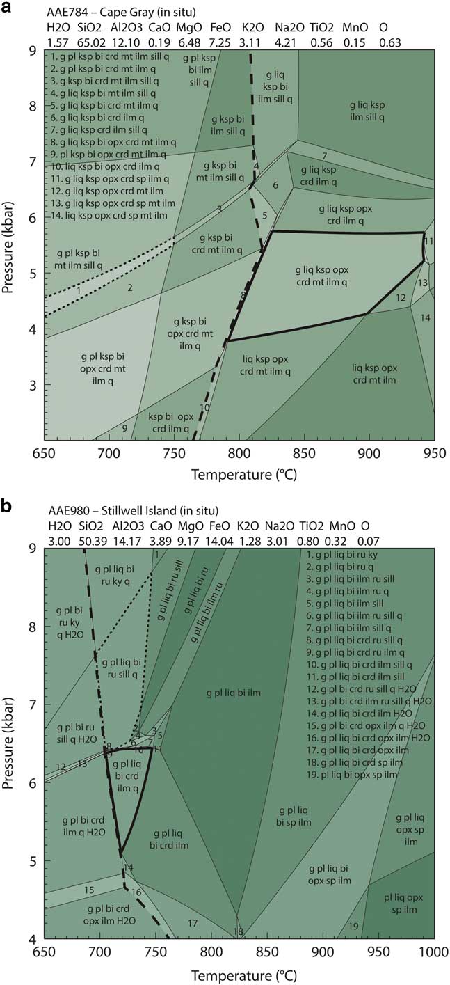
P–T phase equilibria models are provided in Figs 9–11, modal abundance contour models are provided in Fig. 12 and a summary of all calculated P–T conditions is shown in Fig. 13.
Calculated P–T forward models for sample AAE784 from the Cape Gray Gneiss and sample AAE980 from the Stillwell Island metapelite. Bulk compositions used for P–T calculations are provided at the top of the models and are expressed as mole percent. Dashed line indicates solidus. a. The peak assemblage field for AAE784 contains garnet–plagioclase–melt–K-feldspar–cordierite–ilmenite–quartz and is outlined in bold. The field garnet–plagioclase–K-feldspar–biotite–cordierite–magnetite–ilmenite–sillimanite–quartz, outlined with a dotted line and labelled with assemblage 1, indicates the post-peak coarse grained assemblage in this sample. b. The peak assemblage field for AAE980 contains garnet–plagioclase–melt–biotite–cordierite–ilmenite–quartz and is outlined in bold. The field garnet–plagioclase–melt–biotite–rutile–sillimanite–quartz, outlined with a dotted line, indicates the pre-peak coarse grained assemblage in this sample. bi=biotite, chl=chlorite, crd=cordierite, cor=corundum, g=garnet, ilm=ilmenite, ksp=K-feldspar, liq=melt, ru=rutile, mnz=monazite, mt=magnetite, opx=orthopyroxene, pl=plagioclase, q=quartz, ru=rutile, sill=sillimanite.
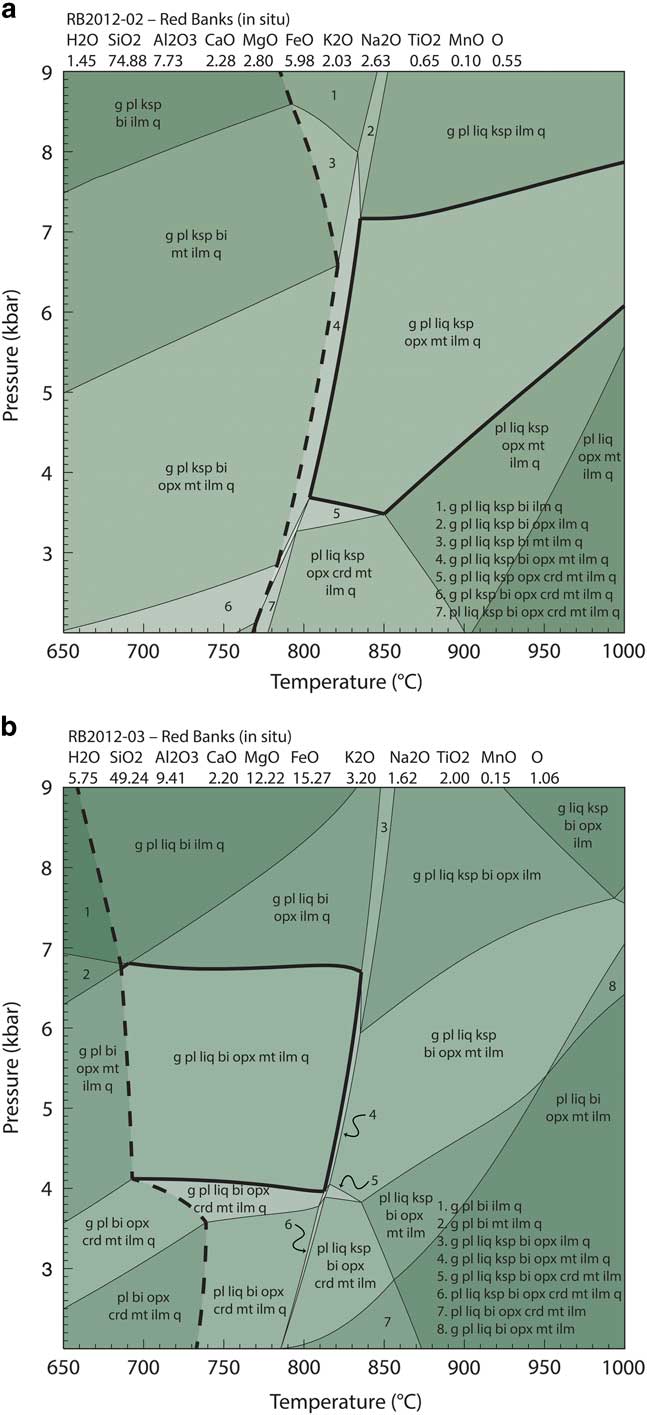
Calculated P–T forward models for samples RB2012-02 and RB2012-03 from the Red Banks Charnockite. Bulk compositions used for P–T calculations are provided at the top of the models and are expressed as mole percent. Dashed line indicates solidus. a. The peak assemblage field for RB2012-02 contains garnet–plagioclase–melt–K-feldspar–orthopyroxene–magnetite–ilmenite–quartz and is outlined in bold. b. The peak assemblage field for RB2012-03 contains garnet–plagioclase–melt–biotite–orthopyroxene–magnetite–ilmenite–quartz and is outlined in bold. bi=biotite, chl=chlorite, crd=cordierite, cor=corundum, g=garnet, ilm=ilmenite, ksp=K-feldspar, liq=melt, mnz=monazite, mt=magnetite, opx=orthopyroxene, pl=plagioclase, q=quartz, sill=sillimanite.
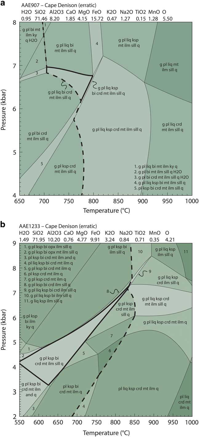
Calculated P–T forward models for erratic samples AAE907 and AAE1233 from Cape Denison. Bulk compositions used for P–T calculations are provided at the top of the models and are expressed as mole percent. Dashed line indicates solidus. a. The peak assemblage field for AAE907 contains garnet–plagioclase–melt–K-feldspar–biotite–cordierite–magnetite–ilmenite–sillimanite–quartz and is outlined in bold. b. The peak assemblage field for AAE1233 contains garnet–plagioclase–melt–K-feldspar–biotite–magnetite–ilmenite–sillimanite–quartz and is outlined in bold. bi=biotite, chl=chlorite, crd=cordierite, cor=corundum, g=garnet, ilm=ilmenite, ksp=K-feldspar, liq=melt, mnz=monazite, mt=magnetite, opx=orthopyroxene, pl=plagioclase, q=quartz, sill=sillimanite.
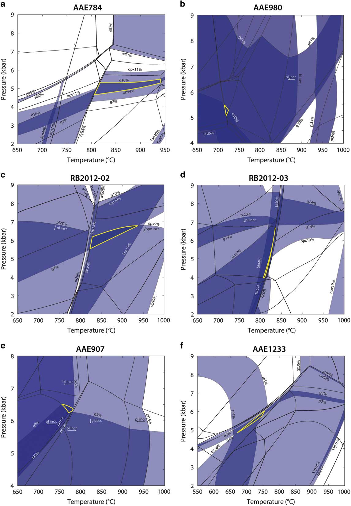
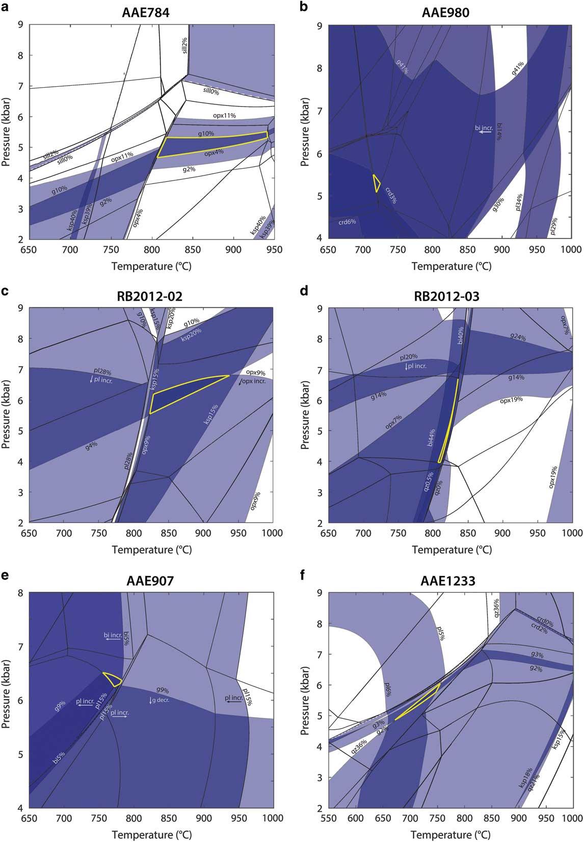
Calculated mineral modal abundance contours. Blue bands represent upper and lower limits on measured mineral abundance estimates for each phase. Mineral abundance contours (upper and lower bound of bands) given for ± 1 standard deviation from mean of peak mineral abundance estimates (Table II), with post-peak minerals removed from estimates and remaining values renormalized. Mineral abundance contours are labelled with mineral and modal abundance. Mineral assemblages as in Figs 9–11. Bold yellow line indicates extent of peak field based on mineral contours.
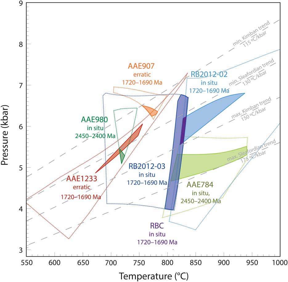
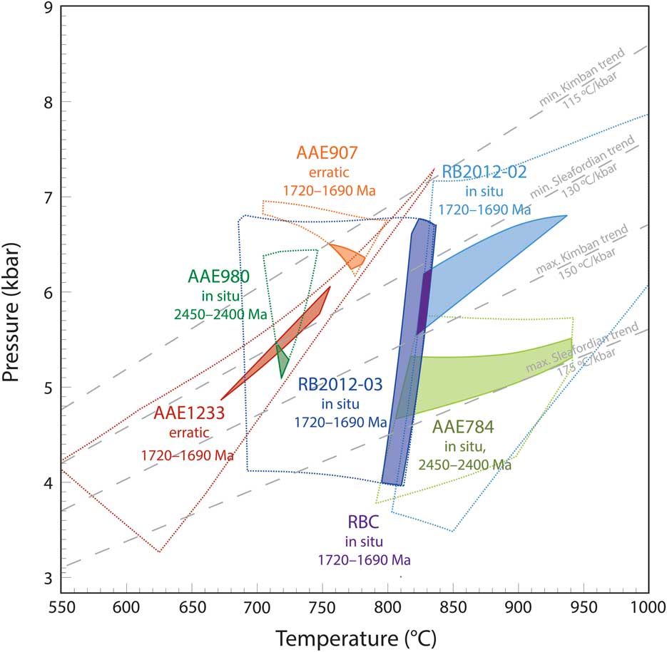
Summary of P–T constraints for all samples. The extent of peak assemblage fields are shown in bold dotted lines for all modelled samples (Figs 9–11). Shaded fields show refined estimates based on modal abundance of peak minerals, as shown in Fig. 12. Opaque purple field shows refined estimate for the Red Banks Charnockite (RBC) from the common overlap of the refined peak fields for samples RB2012-02 and RB2012-03. Samples AAE784 and AAE980 show exclusively 2450–2400 Ma monazite populations. Samples AAE907, AAE1233, RB2012-02 and RB2012-03 show exclusively 1720–1690 Ma monazite populations.
In sample AAE784 (Cape Gray Gneiss, in situ), the inferred peak mineral assemblage garnet–K-feldspar–orthopyroxene–cordierite–magnetite–ilmenite–quartz–melt is stable within the P–T range of 3.8–5.6 kbar and 790–940°C (Fig. 9a). Calculated mineral mode contours used in conjunction with estimated mineral abundances in thin section (Table II) for orthopyroxene and garnet constrain the peak conditions within the peak assemblage field to 4.5–5.2 kbar and 810–940°C (Fig. 12a). Late cordierite, plagioclase and biotite developed in this sample occur to lower pressures and/or lower temperatures than the peak field (Fig. 9a).
In sample AAE980 (Stillwell Island metapelite, in situ), the inferred peak mineral assemblage garnet–plagioclase–biotite–cordierite–ilmenite–quartz–melt is stable within the P–T range of 5.1–6.5 kbar and 700–750°C (Fig. 9b). Calculated mineral mode contours corresponding to the estimated abundance of cordierite thin section (Table II) constrain the peak conditions within the peak assemblage field to between 5.1–5.5 kbar and 710–730°C (Fig. 12b). Pre-peak rutile and sillimanite in this sample occur at higher pressures than the stability field corresponding to the inferred peak mineral assemblage (Fig. 9b).
In sample RB2012-02 (Red Banks Charnockite, in situ), the inferred peak mineral assemblage garnet–plagioclase–K-feldspar–orthopyroxene–magnetite–ilmenite–quartz–melt is stable within the P–T range of 3.5–8.0 kbar and 800–1000°C (Fig. 10a). Calculated mineral mode contours corresponding to estimated mineral abundances of garnet and orthopyroxene in thin section (Table II) constrain the peak conditions within the peak assemblage field to between 5.4–6.8 kbar and 820–940°C (Fig. 12c).
In sample RB2012-03 (Red Banks Charnockite, in situ), the interpreted peak mineral assemblage garnet–plagioclase–biotite–orthopyroxene–magnetite–ilmenite–quartz–melt occurs over the P–T range 4.0–6.8 kbar and 680–830°C (Fig. 10b). Calculated mineral mode contours corresponding to estimated mineral abundances of biotite and quartz in thin section (Table II) constrain the peak conditions within the peak assemblage field to between 4.0–6.8 kbar and 790–830°C (Fig. 12d).
In sample AAE907 (Cape Denison, erratic), the inferred peak mineral assemblage garnet–plagioclase–biotite–cordierite–magnetite–ilmenite–sillimanite–quartz–melt is stable within the P–T range of 6.2–6.9 kbar and 710–800°C (Fig. 11a). Calculated mineral mode contours corresponding to estimated mineral abundances of garnet and plagioclase in thin section (Table II) constrain the peak conditions within the peak assemblage field to between 6.2–6.5 kbar and 760–790°C (Fig. 12e).
In sample AAE1233 (Cape Denison, erratic), the inferred peak mineral assemblage garnet–plagioclase–K-feldspar–biotite–cordierite–ilmenite–sillimanite–magnetite–quartz is stable within the P–T range of 3.2–7.2 kbar and 550–840°C (Fig. 11b). Calculated mineral mode contours corresponding to estimated mineral abundances of garnet, plagioclase and quartz in thin section (Table II) constrain the peak conditions within the peak assemblage field to between 4.8–6.0 kbar and 670–760°C (Fig. 12f).
Discussion
New and existing age constraints from in situ and erratic samples
All the samples dated in this study using in situ monazite U-Pb geochronology come from granulite facies metamorphic rocks, with the exception of samples AAE1233, which is an upper amphibolite facies metamorphic rock, and AAE612, which is a greenschist facies rock with relict granulite facies domains. Within each sample, except AAE612, the monazite ages are unimodal and identical within error regardless of microstructural setting, suggesting that all grains have similar growth histories. In sample AAE612, older monazite ages come from within cordierite grains containing sillimanite and corundum inclusions, interpreted to be part of the relict peak granulite facies assemblage. Furthermore, individual monazite grains in all samples do not show age inheritance or resetting, and agree with the known ages of metamorphism in the Mawson Continent. It is on this basis that the samples are interpreted to record the timing of metamorphism.
Monazite U-Pb geochronology collected from outcropping samples at Cape Gray and Stillwell Island reveals single age populations in the range 2450–2420 Ma (Fig. 8), corresponding to the established timing of the Sleaford event (e.g. Hand et al. Reference Hand, Reid and Jagodzinski2007, Duclaux et al. Reference Duclaux, Rolland, Ruffet, Ménot, Guillot, Peucat, Fanning, Rey and Pêcher2008). In contrast to the in situ coastal samples, ages obtained from the Cape Denison erratics are typically significantly younger (1690–1710 Ma), corresponding to the timing of the Kimban event (e.g. Dutch et al. Reference Dutch, Hand and Kelsey2010). The one exception is sample AAE612, which contains two distinct age populations, the older of which (c. 2390 Ma) is similar to the ages obtained from the in situ samples AAE784 and AAE980, and the younger age population (c. 1710 Ma) approximately coincides with the age populations in the remainder of the dated erratics (Fig. 8) and Palaeoproterozoic sequences west of Cape Denison (Gapais et al. Reference Gapais, Pelletier, Ménot and Peucat2008 and references therein).
Age data from the erratic samples can be interpreted in two ways. One possibility is that in samples AAE907 and AAE1233 inherited 2450–2400 Ma monazite completely recrystallized at c. 1690 Ma. A second possibility is that these two samples did not undergo metamorphism at 2450–2400 Ma. As it is unknown from how far inland the erratics were derived, aside from the absolute geographical limits imposed by the ice drainage basin (Rignot et al. Reference Rignot, Mouginot and Scheuchl2011) it is difficult to definitively interpret the significance of the young ages from these samples.
Polymetamorphism: evidence from geochronology
In erratic sample AAE612, the extensive development of cordierite is interpreted to reflect the younger Kimban event and the domains containing sillimanite and corundum are interpreted to be relict from the older Sleaford event. This interpretation is plausible based on the occurrence of Kimban-aged monazite grains exclusively hosted within the cordierite-rich matrix of the rock, whereas monazite grains with Sleaford ages are hosted by sillimanite–corundum aggregates (Fig. 6). In all other samples, the monazite populations are unimodal, and therefore the preserved mineral assemblages are assumed to reflect one stage of growth coincident with monazite growth. Therefore, the Sleaford-aged mineral assemblages in Antarctic coastal samples are interpreted to have not been reworked during the Kimban event.
In the Australian Mawson Continent, the Sleaford Complex contains a known record of Kimban-aged metamorphic and structural reworking (Dutch et al. Reference Dutch, Hand and Kinny2008, Reference Dutch, Hand and Kelsey2010). Dutch et al. (Reference Dutch, Hand and Kinny2008) showed that mylonitic and migmatitic high-strain zones with Kimban monazite ages occur in Sleaford-aged meta-igneous rocks on the Coffin Bay Peninsula. Approximately 40 km to the south-east at Shoal Point, Dutch et al. (Reference Dutch, Hand and Kelsey2010) showed that boudins in metasedimentary gneisses retain a Sleaford-aged fabric that is discordant to the dominant and enveloping Kimban-aged fabric in the metasedimentary gneisses. On this basis, the record of reworking along the southernmost coast of Eyre Peninsula changes from discrete or ‘patchy’ to potentially more pervasive as a function of rock rheology.
Such field relationships highlight the spatially complex way that polymetamorphism in basement terranes can be recorded and may go some way to explaining why the in situ Antarctic coastal samples do not record Kimban-aged reworking, in contrast to other proximal locations along the Antarctic coast (Oliver & Fanning Reference Oliver and Fanning2002, Di Vincenzo et al. Reference Di Vincenzo, Talarico and Kleinschmidt2007, Duclaux et al. Reference Duclaux, Rolland, Ruffet, Ménot, Guillot, Peucat, Fanning, Rey and Pêcher2008 and references therein). Previous studies proposed that the record of the 1720–1690 Ma Kimban event was limited to narrow, fluid-bearing, anastomosing shear zones concentrated along the edges of the basement domain (Oliver & Fanning Reference Oliver and Fanning2002, Duclaux et al. Reference Duclaux, Rolland, Ruffet, Ménot, Guillot, Peucat, Fanning, Rey and Pêcher2008, Gapais et al. Reference Gapais, Pelletier, Ménot and Peucat2008 and references therein). In the case of Dutch et al. (Reference Dutch, Hand and Kinny2008, Reference Dutch, Hand and Kelsey2010), the polymetamorphic history was only revealed through geochronology. Therefore, the exclusively 2450–2400 Ma ages in the Antarctic coastal outcrops studied here (AAE784, AAE980) may reflect fortuitous sampling of the outcropping rock by the 1911–14 AAE, or fortuitous selection of samples from the archived collection. This effectively implies that there are regions of outcrop indistinguishable in the field that record either extensive or no reworking during the Kimban. Our preferred interpretation is that chemical heterogeneities caused by the depletion or accumulation of melt led to spatially irregular retrogression occurring either during the waning/exhumation stages of the Sleaford event or between the two high metamorphic grade events. The reactive contrast between retrogressed parts of rocks versus residual granulite during later (Kimban-aged) reheating is a mechanism for creating the inconsistencies in the record of ages and metamorphic reworking.
Further clarification of the relationships between these two events could be elucidated by the use of other accessory minerals, including zircon, to bring together age data from other geochronometers. Furthermore, trace element signatures in accessory minerals could be used to definitively link mineral growth (e.g. garnet) with timing of metamorphism (e.g. Buick et al. Reference Buick, Hermann, Williams, Gibson and Rubatto2006).
Polymetamorphism: evidence from microstructural andP–T constraints
The P–T records in high metamorphic grade terranes, such as the Mawson Continent, that have undergone multiple high-grade events are challenging to interpret based on their metamorphic record. This is because later mineral assemblages variably overprint earlier metamorphic assemblages, and thus it is often difficult to determine whether one or more events produced the visual mineralogical record. If a temporally unrelated event was responsible for the generation of the overprinting mineral assemblage(s), the overall P–T evolution could incorrectly be interpreted as the result of a single event, which would impact tectonic models based on the P–T path record.
Fortunately, in the study region it is possible to uniquely constrain the metamorphic P–T conditions of the younger, Kimban-aged metamorphism using the metamorphic record in the Red Banks Charnockite, the protolith of which intruded metapelitic granulites at 2011±7 Ma (Jagodzinski et al. Reference Jagodzinski, Reid and Hand2012) and therefore cannot record 2450–2400 Ma metamorphism. Metamorphic zircon in the Red Banks Charnockite gave a unimodal age of 1722±7 Ma (Jagodzinski et al. Reference Jagodzinski, Reid and Hand2012) and the metamorphic monazite age is 1720±9 Ma (Fig. 8), suggesting metamorphism during the early Kimban event (e.g. Dutch et al. Reference Dutch, Hand and Kelsey2010) with no younger overprint. The P–T modelling of two garnet–orthopyroxene-bearing migmatite samples from the Red Banks Charnockite provides a large range of possible temperatures, mostly because there is uncertainty of whether quartz and K-feldspar are part of the peak assemblage in sample RB2012-03 (Figs 10 & 12). If quartz is interpreted as part of the peak assemblage in RB2012-03, the peak P–T conditions for the Kimban event, as constrained by the intersection of the peak P–T conditions for samples RB2012-02 and RB2012-03, are 5.6–6.2 kbar and 810–830°C (see purple shaded area in Fig. 13). The results of P–T modelling from the Red Banks Charnockite provide a reference with which to interpret the P–T record developed in the older granulites in the Sleaford–Cape Denison region. They also provide a reference to compare with the modelled metamorphic conditions in the erratic samples AAE907 and AAE1233 with only Kimban-aged monazite populations.
Figure 13 shows the peak assemblage fields in P–T space for all samples in this study. The peak conditions calculated here for sample AAE907 are slightly higher grade than the amphibolite facies conditions previously reported for the Kimban event along the George V Coast (4–6 kbar and 700–750°C, Ménot et al. Reference Ménot, Pecher, Rolland, Peucat, Pelletier, Duclaux and Guillot2005 and references therein). The peak metamorphic conditions for the Red Banks samples, constrained by matching observed to calculated peak mineral modes (Figs 12c, 12d & 13), correspond to apparent thermal gradient trends of 130–150°C kbar-1, whereas for the remaining samples with Kimban ages the apparent thermal gradients are 115–135°C kbar-1. For samples with only Sleaford ages (AAE784, AAE980) the apparent thermal gradients are 130–175°C kbar-1. The spread of peak P–T conditions for the Antarctic coastal samples (AAE784, AAE980) are arguably slightly lower pressure than the peak P–T conditions for the Red Banks samples (as defined by the common overlap of the conditions from RB2012-02 and RB2012-03) and Antarctic erratic samples with Kimban-aged monazite; however, the apparent thermal trends for samples of both ages have considerable overlap. These findings suggest one of two possibilities: i) the 2450–2400 Ma event as recorded in coastal samples AAE784 and AAE980 was of very similar thermal character to the 1720–1690 Ma event, or ii) the silicate assemblages recorded in the samples that contain 2450–2400 Ma monazite actually record 1720–1690 Ma P–T conditions, despite not recording this later event in their monazite age populations. The first possibility is the simplest interpretation as it allows coupling of monazite age data to P–T conditions and silicate mineral assemblages (e.g. Kelsey et al. Reference Kelsey, Hand, Clark and Wilson2007). The second possibility requires that the behaviour of monazite was completely independent of that of silicate mineral assemblages. In this scenario, all P–T data from this study (Fig. 13) is Kimban-aged. Total decoupling of monazite behaviour and U-Pb ages from that of the silicate minerals in rocks is not typically reported. Instead, monazite geochemistry is typically linked to geochemical signatures or patterns in silicate minerals, such as garnet or feldspar, in partially melted as well as subsolidus rocks (e.g. Kelly et al. Reference Kelly, Harley and Möller2012). Therefore, the first of these possibilities is our preferred interpretation. That the thermal character of successive events involving upper amphibolite–granulite facies metamorphism is similar is not surprising given that formation of granulites in particular requires elevated thermal gradients (e.g. Brown Reference Brown2007).
Subice geology of inland Antarctica
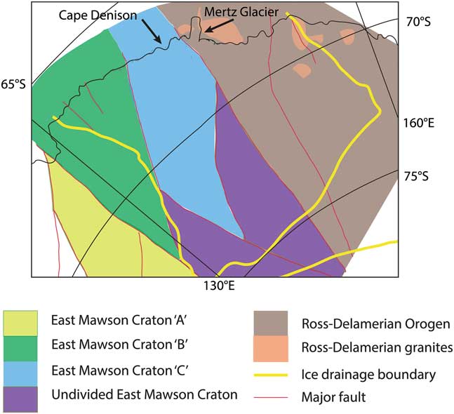
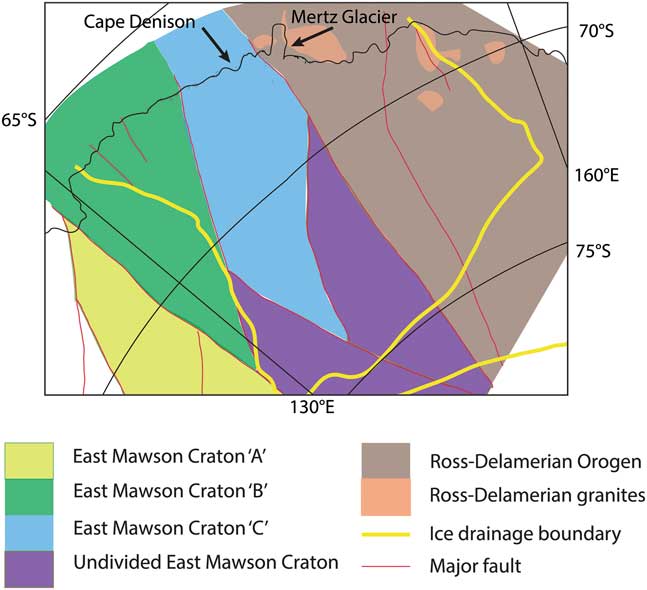
Geophysical data was used to interpret that the Mawson Continent extends inland for more than 1000 km south of the George V–Terre Adélie coast, separated in the east from the Ross–Delamerian Orogeny by the Mertz Fault and in the west by the Albany–Fraser system (Fig. 14; Aitken et al. Reference Aitken, Young, Ferraccioli, Betts, Greenbaum, Richter, Roberts, Blankenship and Siegert2014). The ice drainage basin of George V Land–Terre Adélie extends inland c. 600 km (Rignot et al. Reference Rignot, Mouginot and Scheuchl2011), draining the interpreted East Mawson Craton ‘B’ and ‘C’ of Aitken et al. (Reference Aitken, Young, Ferraccioli, Betts, Greenbaum, Richter, Roberts, Blankenship and Siegert2014 fig. 3), and covers a small portion of ‘Undivided East Mawson Craton’ at its southernmost limit. East Mawson Craton ‘C’ corresponds to the Palaeoproterozoic and Archean coastal geology of this study, whereas East Mawson Craton ‘B’ corresponds to the younger, magmatic-dominated c. 1620 Ma St Peter and/or c. 1590 Ma Hiltaba Suites. On the basis of our earlier interpretation of geochronology from erratic samples, the subice geology of East Mawson Craton ‘C’ is conceivably dominated by post-Sleaford sequences that record Kimban metamorphism and deformation. In this interpretation these sequences were not present to record the Sleaford event. However, the two monazite age populations in erratic sample AAE612 show that the subice geology also comprises at least some pre-Sleaford metasedimentary sequences. In conclusion, the subice geology of the Mawson Continent is a pre-Sleaford-aged terrane with a cover sequence reworked during the Kimban event. Our study provides a platform for conducting further work on glacial erratics to further delineate the subice geology of eastern Antarctica.
Geophysical interpretation map of the Antarctic Mawson Continent with ice drainage basin extent (after Rignot et al. Reference Rignot, Mouginot and Scheuchl2011, Aitken et al. Reference Aitken, Young, Ferraccioli, Betts, Greenbaum, Richter, Roberts, Blankenship and Siegert2014). Tectonic block names (Mawson Craton) after Aiken et al. Reference Aitken, Young, Ferraccioli, Betts, Greenbaum, Richter, Roberts, Blankenship and Siegert2014.
Conclusions
In situ and erratic samples from the central Mawson Continent record two monazite metamorphic age populations at 2450–2400 Ma and 1720–1690 Ma, which correspond to the timing of the Sleaford and Kimban events, respectively. In situ samples from the Antarctic coast record exclusively 2450–2400 Ma ages. Erratic samples record 1720–1690 Ma ages, with the exception of erratic sample AAE612 that records both monazite age populations. Calculated P–T conditions of peak metamorphism are granulite facies across all samples, with the exception of sample AAE1233, which records upper amphibolite facies conditions. The Kimban event corresponds to apparent thermal gradients of 130–145°C kbar-1, uniquely constrained by the Red Banks Charnockite, which intruded the host Carnot Gneiss at c. 2011 Ma. Mineral assemblages interpreted as 2450–2400 Ma in age suggest the peak of Sleaford metamorphism was arguably lower pressure, similar temperature and of higher apparent thermal gradient, with a higher pressure pre-peak history. However, the overall P–T characters for the two events are similar. The spatially ‘patchy’ record of reworking is interpreted to be due to heterogeneities in the depletion or accumulation of melt and subsequent retrogression occurring either during the waning/exhumation stages of the Sleaford event or between the two (high-grade) events.
Acknowledgements
The authors thank P. Pitra, F. Korhonen, S. Harley and J. Halpin for helpful and insightful reviews that greatly improved the quality of this manuscript. C. Atkin is thanked for swift editorial handling. Thanks are due to the staff at Adelaide Microscopy for their assistance with analytical work and S. Mertzman at Franklin and Marshall College for geochemical analysis. This work was supported by DP160101006 and forms a contribution to AAS project 4191. An Australian Government Research Training Program Scholarship and a Vacation Research Scholarship from the University of South Australia supported MAW. RAD publishes with the permission of the Director, Geological Survey of South Australia.
Author contributions
MAW completed modelling, data collection and analysis, and wrote the paper. DEK contributed to the design of the study, data interpretation and preparation of the paper. MH conceived the study and contributed to the design of the study, field sampling, observations, data interpretation and preparation of the paper. TR assisted with geochronology data and interpretation. LJM and NMT assisted with phase equilibria modelling and interpretation. RAD contributed field sampling, observations and interpretation.
Supplemental material
Supplemental appendices, tables and figures will be found at http://dx.doi.org/10.1017/S0954102017000451.